Download Solving optimization problems

Solving Optimization Problems By
the Optimization Program
INVERSE
(FOR VERSION 3.18)
Igor Grešovnik
Ljubljana, 13 March, 2008
INVERSE 3.18
6.1: Optimization And Inverse Analyses / Table of contents
Contents:
6.
Optimization And Inverse Analyses .......................................................................... 3
6.1
6.1.1
6.1.2
6.1.3
6.1.4
6.1.5
6.2
Definition of Optimization Problem and its Solution ................................................3
Basic Terms .............................................................................................................................3
Installing and running the optimization program Inverse ........................................................4
Definition of the Problem in the Command file ......................................................................5
Defining the Direct Analysis ...................................................................................................5
Implicit Gradient Calculation ..................................................................................................6
Optimization algorithms...............................................................................................9
6.2.1
optfsqp { numob numnonineq numlinineq numnoneq numlineq eps epseqn maxit grad
initial < lowbound upbound > } .........................................................................................................9
6.2.2
minsimp { tolx tolf maxit printlevel initial step }...................................................................10
6.2.3
nlpsimp { numconstr tolx tolf tolconstr maxit printlevel initial step } ...................................11
6.2.4
NLPSimpS, nlpsimps { numconstr tolx tolf tolconstr maxit printlevel initial step }.............12
6.2.5
nlpsimpbound0 { numconstr tolx tolf tolconstr maxit printlevel initial step bignum <
lowbounds upbounds bignum < kpen kconstr < numviolations maxresid > > > }..............................12
6.2.6
solvopt { numconstr numconstreq tolx tolf tolconstr maxit lowgradstep initial }..................16
6.3
Older functions for optimization ...............................................................................17
6.3.1
inverse { methodspec params }..............................................................................................17
6.3.2
optfsqp1 { numob numnonineq numlinineq numnoneq numlineq eps epseqn maxit grad {
initial } { lowbound } { upbound } }.....................................................................................................18
6.3.3
optsimplex { tol maxit startguess } ........................................................................................19
6.4
6.4.1
6.4.2
6.5
6.5.1
7.
Auxiliary tools .............................................................................................................20
Testing the Direct Analysis....................................................................................................20
Tabulating Functions .............................................................................................................21
Approximation tools ...................................................................................................27
Smooth approximation...........................................................................................................27
Uniform File Interface Between Optimization and Analysis Programs................ 29
7.1
Interpreter functions...................................................................................................30
7.2
File Formats.................................................................................................................36
7.2.1
7.2.2
7.2.3
File format for analysis request (analysis input file)..............................................................37
File format for analysis results (analysis output file).............................................................37
XML formats .........................................................................................................................39
7.3
Solution Scheme ..........................................................................................................44
7.4
Demonstrative example ..............................................................................................45
7.4.1
7.4.2
7.4.3
List of files.............................................................................................................................45
Running the example and using custom analysis program ....................................................46
Using a different analysis program........................................................................................47
2
INVERSE 3.18
6.1: Optimization And Inverse Analyses / Definition of Optimization Problem and its Solution
6. OPTIMIZATION AND INVERSE ANALYSES
6.1 Definition of Optimization Problem and its Solution
6.1.1 Basic Terms
We state the optimization problem quite generally as
minimise
f (x ),
x ∈ IR n
subject to
ci ( x ) ≤ 0, i ∈ I
and
c j ( x ) = 0, j ∈ E ,
where
lk ≤ xk ≤ uk , k = 1, 2, ..., n .
(6.1)
Function f is called the objective function, ci and cj are called constraint functions
and lk and uk are called upper and lower bounds. The second and third line of the equation
are referred to as inequality and equality constraints, respectively (with I and E being the
corresponding inequality and equality index sets). We will collectively refer to f, ci , i ∈ I
and ci , i ∈ E as constraint functions. Sometimes the algorithm can in addition take the
advantage of explicitly stated eventual linear constraint functions, such as in the case of
fsqp.
The set of points in which all constraints are satisfied is called feasible region.
Solution of the problem is contained in the feasibleregion.
3
INVERSE 3.18
6.1: Optimization And Inverse Analyses / Definition of Optimization Problem and its Solution
6.1.2 Installing and running the optimization program Inverse
In order to run Inverse, you need an executable for your platform and a I.G.’s
software home directory referred to as ighome (which is default name for this directory).
The executable is usually put to ighome.
Installation procedure is simple:
1. Copy the I.G.’s software home directory (ighome) somewhere on your
hard disk, (e.g. in “c:\” on windows, in this case the I.G.’s software home
would be “c:\ighome”). The location must be such that all users have read
& write access to files in the directory.
2. Set the value of environment variable IGHOME to the location of the
I.G.’s software directory (ighome). Note that the case matters on some
platforms. The environment variable must be created if it does not yet
exist, otherwise its value must be changed such that it contains the
absolute path of ighome.
3. Add the bin subdirectory of the software home directory (ighome) to the
path environment variable. You can usually use the previously defined
variable IGHOME (e.g. %IGHOME%\bin on Windows or $IGHOME/bin
on Unix-like systems) to refer to this directory.
4. Copy the executable for your platform to the bin subdirectory of ighome.
5. Now you can run the program in a terminal window. Usually you will
have to re-open the terminal window so that the new environment
variables will take effect.
You run Inverse by typing the name of its executable followed by command-line
arguments. Usually the first (and often the only) argument is the name of the command
file (or path, if the file is not contained in the current directory). Command file must
contain instructions that are executed by Inverse.
On Windows, for example, provided that the file name of Inverse executable is
inverse.exe and there is a command file named opt.cm in the current directory, you would
run the program in the following way:
inverse opt.cm
The program, software home directory and some additional files can be
downloaded from the download section of the Inverse home page.
4
INVERSE 3.18
6.1: Optimization And Inverse Analyses / Definition of Optimization Problem and its Solution
6.1.3 Definition of the Problem in the Command file
The optimization problem and its solution procedure must be defined in the shell
command file, which is interpreted by the interpreter.
The command file typically consists of three parts: the preparation part, the
analysis block and the final action part. In the preparation part variables are typically
allocated, data initialized and functions defined for use at a later time. The analysis block
defines how direct analysis is performed. This block is interpreted every time the direct
analysis is performed, either run from within some algorithm or as a consequence of user
request. In the action part the optimization algorithms that lead to problem solution are
run. Test analyses at different parameter sets or some other tests (e.g. tabulating of the
objective function) can also be run in this part.
The preparation part and analysis block can usually be swapped. Individual
allocations and definitions can be performed right before they are used, although the
command file usually looks clearer if this is done in one place. The user must be careful
about putting definitions and allocations in the analysis block because this block is
iteratively interpreted. What concerns tasks that do not need to be performed in every
analysis, it is better if they are invoked outside the analysis block so that they are
performed only once.
6.1.4 Defining the Direct Analysis
The term “direct analysis” refers to the evaluation of the objective and constraint
functions and possibly their gradients at a given set of optimization parameters. User
defines how the direct analysis is performed in the analysis block of the shell command
file. This is the block of code in the argument block of the analysis command, i.e. within
the curly brackets that follow this command.
The analysis block is interpreted by the shell interpreter every time the direct
analysis is performed. Direct analysis can be called by an optimization algorithm or by
some other function invoked by the interpreter. Typical examples are tabulating functions
or the analyse function for performing test direct analyses.
Data transfer between the direct analyses and the functions that invoke them is
implemented through global shell variables with a pre-defined meaning. The shell takes
care that the current set of optimization parameters is always in the vector variable
parammom when the direct analysis is invoked. In the analysis block the user can
therefore obtain parameter values from this variable using the interpreter and expression
evaluator functions for accessing variables. In the similar way it is expected that after the
direct analysis is performed its results will appear in the appropriate global shell
variables. User must take care of that in the analysis block by storing results in these
variables. For example, value of the objective function must appear in scalar variable
objectivemom, values of constraint functions must appear in scalar variable
constraintmom, objective function gradient in vector variable gradobjectivemom,
5
INVERSE 3.18
6.1: Optimization And Inverse Analyses / Definition of Optimization Problem and its Solution
gradients of constraint functions in vector variable gradconstraintmom, simulated
measurements (in the case of inverse analyses) in vector variable measmom, etc. These
variables with a pre-defined meaning are treated just like other user-defined variables and
the same functions can be used for their manipulation. There are however some
particularities in behaviour of variable manipulation functions in the case of variables
with a pre-defined meaning. Rules are more or less the same, there is only some
additional intelligence incorporated, which enables user not to specify dimensions that
are already known to the shell. For details, see the “Shell Variables with a Pre-defined
Meaning” chapter of the “User Defined Variables in the Optimization Shell Inverse”
manual.
Within the analysis block the user is expected to run a numerical simulation with
parameters found in vector parammom, combine its results to evaluate the requested
function values (objective and constraint functions and their derivatives) and store these
results in the appropriate variables with a pre-defined meaning. This can include a
number of sub-tasks, for example parameter dependent domain transformation in the case
of shape optimization problems (this is reduced to finite element mesh transformation in
some cases). Interfacing the simulation programme, i.e. changing input data according to
parameter values, running the programme and obtaining results, is usually an important
issue, as well as combining of these partial results according to problem definition in
order to derive final results. Several modules of the shell provide tools for performing
such sub-task, and the user can combine these tools using the file interpreter according to
the character of problems that are being solved.
All tools and algorithms of the shell are accessed through the shell file interpreter.
This, together with the expression evaluator (the “calculator”) and interpreter flow
control functions, gives the user a great flexibility at defining different optimization
problems and also the solution procedures. The shell is in the first place designed for use
with simulation programmes. For test purposes, however, the user can define
optimization problems in such way that evaluation of objective and other functions do not
include numerical simulation. The functions are in this case defined analytically using
shell variables and expression evaluator. Such examples can be found in the directory of
training examples (subdirectory “opt”).
6.1.5 Implicit Gradient Calculation
Some optimization algorithms need gradients of the objective and constraint
functions beside their values. Most commonly, these should be calculated in the analysis
block and stored in the appropriate pre-defined variables (e.g. gradobjectivemom or
gradconstraintmom, see the manual on variables, chapter on pre-defined variables). This
essentially means that the algorithm for calculation of the objective and constraint
functions must be differentiated with respect to the design parameters. This is sometimes
difficult to achieve, especially when some numerical simulation is used as a “black box”
and the user does not have access to its source code.
6
INVERSE 3.18
6.1: Optimization And Inverse Analyses / Definition of Optimization Problem and its Solution
The derivatives can always be obtained numerically e.g. 1 by sequentially
perturbing values of individual parameters, calculating the functions at perturbed
parameters and dividing the difference with respect to the response at original parameters
by the perturbation (i.e. difference in parameter value or step size). This can be eventually
programmed within the analysis block of the interpreter. Doing so, however, can
significantly reduce the clearness and readability of the analysis block.
The tools have been providing for automatic implicit numerical calculation of the
derivatives. When implicit derivative calculation is switched on, on any request for
performing the analysis at given parameter values, the (non-derivative) analysis is
actually performed with the original and perturbed parameter values. Numerical
approximation of gradients of the objective and constraint functions is calculated on the
basis of the results and stored to the appropriate pre-defined variables (most commonly
gradobjectivemom and gradconstraintmom) together with function values at the original
parameters of the request (objectivemom and constraintmom are commonly used to store
these).
The interpreter functions for providing implicit numerical gradient calculation are
described below.
6.1.5.1 analysisnumgradfdvec { stepvec }
Installs the implicit numerical calculation of gradients of the objective and
constraint functions (if defined) with respect to optimization parameters by the forward
difference scheme. This applies to the functions that are calculated by the direct analysis
direct analysis, which includes interpretation of the analysis block. stepvec must be a
vector value argument that specifies the step size for each parameter. Its dimension must
therefore be the same as the number of parameters (i.e. the dimension of the pre-defined
vector parammom). If stepvec is not specified, then the default step size (10-4) is taken for
derivation with respect to all parameters. It is usually a very bad idea not to specify the
step sizes because the accuracy of the derivatives depend essentially on it, and the
optimal step size may vary drastically from case to case since it depends on scaling of the
design parameters and on the level of noise of the differentiated functions.
After the call to the function, every direct analysis at a given set of parameters is
replaced by a number of plain analyses. The first one is performed at the requested
parameters and n others are performed at the parameter sets in which one parameter is
perturbed by the appropriate step size as specified by stepvec, n being the number of
parameters. After this, the function values calculated with the requested parameter values
are stored as usual (e.g. in the pre-defined variables objectivemom or/and
constraintmom). In addition, numerical approximations to the parameter gradients of
these values are calculated and stored at the appropriate place 2 (e.g. in the pre-defined
1
This scheme is called the finite difference method. There are also more complex schemes for numerical
derivative calculation, all of which include repeating calculation of function values at a number of
perturbed parameters, but differ significantly in sampling strategies and underlying mathematics.
Description of these schemes exceeds the scope of this manual.
2
This would normally be done explicitly by the appropriate interpreter code in the analysis block.
7
INVERSE 3.18
6.1: Optimization And Inverse Analyses / Definition of Optimization Problem and its Solution
variables gradobjectivemom and gradonstraintmom). See the manual on variables,
chapter on pre-defined variables for more details regarding the meaning of specific predefined variables and rules for their manipulation.
The accuracy of the numerically calculated derivatives crucially depends on the
step size. The derivative calculation is mathematically exact for linear functions, and
therefore there are two sources of error. The first one is because the function is normally
not linear and this contributes larger errors where the step size gets large and the function
deviates more from the linear model. The second source is due to the noise in the function
value. If there is no other source of noise, at least the function values are inexact because
of finite precision that is used for all computer operations. Errors in calculated derivatives
that come from this source are amplified when the step size is reduced, and die away
when the step size gets large compared to the amplitude of noise. Therefore, there exists
an optimal step size which is large enough with respect to noise amplitude and yet small
enough that the function is adequately approximated by a linear model within the step
size. The user should provide the step size that is not necessarily optimal, but is a good
compromise for both sources of error. When it is hard to estimate the level of noise, the
step size should be taken that is a bit smaller than the tolerance for the optimum, and the
tolerance should be set rather conservatively in order to avoid failure of algorithms due to
excessive noise.
6.1.5.2 analysisnumgradfd { stepsize }
Does the same as analysisnumgradfdvec, except that the step size for all
parameters are set equal to stepsize, which is a scalar value argument. If stepsize is not
specified then a default step size (10-4) is taken. However, it is usually a very bad idea not
to specify the step size because the accuracy of the derivatives depend essentially on it,
and the optimal step size may vary drastically from case to case since it depends on
scaling of the design parameters and on the level of noise of the differentiated functions.
6.1.5.3 analysisplain { }
Cancels the implicit numerical differentiation of the objective function (and
constraint functions if defined) and places instead the original analysis function, which
performs the direct analysis (including interpretation of the analysis block) at only one set
of design parameters.
6.1.5.4 analysisnumgradprn { doprn }
If the counter value argument doprn is different than 0 then reporting on gradient
calculation is switched on, which can be used for control.
8
INVERSE 3.18
6.2: Optimization And Inverse Analyses / Optimization algorithms
6.2 Optimization algorithms
6.2.1 optfsqp { numob numnonineq numlinineq numnoneq numlineq
eps epseqn maxit grad initial < lowbound upbound > }
Performs the fsqp (feasible sequential quadratic programming) optimization
algorithm of Craig Lawrence, Jian L. Zhou and Andre Tits, which is the basic and most
powerful nonlinear programming algorithm built in Inverse.
Arguments:
• numob – number of objective functions (should normally be 1) – counter value
argument.
• numnonineq - number of non-linear inequality constraints – counter value
argument.
• numlinineq - number of linear inequality constraints – counter value argument.
• numnoneq - number of non-linear equality constraints – counter value argument.
• numlineq - number of linear equality constraints – counter value argument.
• eps - final norm requirement for the Newton direction – scalar value argument.
• epseqn - maximum violation of nonlinear equality constraints at an optimal point.
Both criteria must be satisfied to stop the algorithm (the second one is in effect
only if there are equality constraints) – scalar value argument.
• maxit - maximum number of iterations – counter value argument.
• grad - specifies if gradients are provided by the direct analyses (1) or should be
calculated numerically (0) – counter value argument.
• initial - initial guess – vector value argument.
• lowbound – lower bounds on parameters – vector value argument.
• upbound - upper bounds on parameters – vector value argument.
If vector value arguments lowbound and upbound are not specified then
parameters are not bounded below or above. If they are specified then those components
for which the corresponding components of lowbound are greater or equal to the
corresponding components of upbound are not bounded.
Note:
Inequality constraints are stated as in (6.1), namely
c (x ) ≤ 0, j ∈ I ,
j
(6.1)
where cj are the constraint functions whose value is expected from the analysis function.
9
INVERSE 3.18
6.2: Optimization And Inverse Analyses / Optimization algorithms
In variables which hold values or derivatives of constraint functions, these must
appear in the appropriate order, the same as in the argument block of the function. First
must be non-linear inequality constraints, then linear inequality constraints, then nonlinear equality constraints and finally linear equality constraints (if any of these are
specified, of course).
Remarks:
See introductory section for how the problem should be defined! You can also
take a look at inquick2.pdf, which can be obtained at
http://www.c3m.si/inverse/doc/other/index.html .
A detailed description of the fsqp algorithm can be found at
http://www.isr.umd.edu/Labs/CACSE/FSQP/fsqp.html .
6.2.2 minsimp { tolx tolf maxit printlevel initial step }
Performs the non-gradient unconstrained minimization algorithm based on the
Nelder-Mead simplex method. This is a non-gradient algorithm suitable also for nondifferentiable and even non-continuous functions that have a well defined unconstrained
minimum. The basic principle is similar to the Nelder-Mead simplex algorithm.
• tolx - tolerance on optimal parameters (approximate). It is a vector value
argument, a tolerance is specified for each co-ordinate. If vector dimension is less
than the problem dimension then missing components are replaced by the first
component. For components that are 0, no tolerance is imposed.
• tolf - tolerance on on optimal value of the objective function (scalar argument). If
it is 0 then this tolerance is not imposed.
• maxit – maximal number of iterations (counter argument)
• printlevel – the level of output produced (counter argument). 0 or less is replaced
by 2.
o 1 - data about arguments and optimization results are printed.
o 2 – basic information about iterations and more detailed information about
results are also printed.
o 3 – simplex (co-ordinates of apices and values of the objective function) is
also printed during iterations and at the
o 4 – Complete results are printed, included values of the constraint
functions
o 5 – at the end, all results of all analyses are also printed. Sets of results in
all simplices over al iterations are also printed in the list form readable by
Mathematica.
• initial – initial guess (vector value parameter)
10
INVERSE 3.18
6.2: Optimization And Inverse Analyses / Optimization algorithms
•
step – step sizes in different directions used to create the initial simplex (vector
value parameter)
Optimal parameters are written to paramopt and optimal value of the objective
function to objectiveopt. Storage of other functions or gradients is not guaranteed.
Remarks:
See introductory section for how the problem should be defined! You can also
take a look at inquick2.pdf, which can be obtained at
http://www.c3m.si/inverse/doc/other/index.html .
6.2.3 nlpsimp { numconstr tolx tolf tolconstr maxit printlevel initial
step }IOptLib
Performs the basic non-linear constraint simplex optimization algorithm of
Igor Grešovnik. This is a non-gradient algorithm suitable also for non-differentiable and
even non-continuous functions that have a well defined constrained minimum. The basic
framework is similar to the Nelder-Mead simplex algorithm.
• numconstr - the number of constraints (equality + inequality), counter argument
• tolx - tolerance on optimal parameters (approximate). It is a vector value
argument, a tolerance is specified for each co-ordinate. If vector dimension is less
than the problem dimension then missing components are replaced by the first
component. For components that are 0, no tolerance is imposed.
• tolf - tolerance on on optimal value of the objective function (scalar argument). If
it is 0 then this tolerance is not imposed.
• tolconstr - tolerance for constraint residuum (scalar argument; if it is 0 then none
of the constraints may be violated in the solution)
• maxit – maximal number of iterations (counter argument)
• printlevel – the level of output produced (counter argument). 0 or less is replaced
by 2.
o 1 - data about arguments and optimization results are printed.
o 2 – basic information about iterations and more detailed information about
results are also printed.
o 3 – simplex (co-ordinates of apices and values of the objective function) is
also printed during iterations and at the
o 4 – Complete results are printed, included values of the constraint
functions
o 5 – at the end, all results of all analyses are also printed. Sets of results in
all simplices over al iterations are also printed in the list form readable by
Mathematica.
• initial – initial guess (vector value parameter)
11
INVERSE 3.18
6.2: Optimization And Inverse Analyses / Optimization algorithms
•
step – step sizes in different directions used to create the initial simplex (vector
value parameter)
Optimal parameters are written to paramopt and optimal value of the objective
function to objectiveopt. Storage of other functions or gradients is not guaranteed.
Note:
Inequality constraints are stated as
c (x ) ≤ 0, j ∈ I
j
(6.2)
where cj are the constraint functions whose value is expected from the analysis function.
Remarks:
See introductory section for how the problem should be defined! You can also
take a look at inquick2.pdf, which can be obtained at
http://www.c3m.si/inverse/doc/other/index.html .
6.2.4 NLPSimpS, nlpsimps { numconstr tolx tolf tolconstr maxit
printlevel initial step }
A variant of the constraint nonlinear simplex method of Igor Grešovnik which
ranges analysis results with violated constraints by the sum of constraint residuals. This is
a non-gradient algorithm suitable also for non-differentiable and even non-continuous
functions that have a well defined constrained minimum. The basic principle is similar to
the Nelder-Mead simplex algorithm.
Arguments are the same as for nlpsimp.
6.2.5 nlpsimpbound0 { numconstr tolx tolf tolconstr maxit printlevel
initial step bignum < lowbounds upbounds bignum < kpen kconstr <
numviolations maxresid > > > }IOptLib
Performs the basic non-linear constraint simplex optimization algorithm of
Igor Grešovnik. This is a non-gradient algorithm suitable also for non-differentiable and
even non-continuous functions that have a well defined constrained minimum. The basic
framework is similar to the Nelder-Mead simplex algorithm.
• numconstr - the number of constraints (equality + inequality), counter argument
12
INVERSE 3.18
6.2: Optimization And Inverse Analyses / Optimization algorithms
•
•
•
•
•
•
•
•
•
•
•
•
•
tolx - tolerance on optimal parameters (approximate). It is a vector value
argument, a tolerance is specified for each co-ordinate. If vector dimension is less
than the problem dimension then missing components are replaced by the first
component. For components that are 0, no tolerance is imposed.
tolf - tolerance on on optimal value of the objective function (scalar argument). If
it is 0 then this tolerance is not imposed.
tolconstr - tolerance for constraint residuum (scalar argument; if it is 0 then none
of the constraints may be violated in the solution)
maxit – maximal number of iterations (counter argument)
printlevel – the level of output produced (counter argument). 0 or less is replaced
by 2.
o 1 - data about arguments and optimization results are printed.
o 2 – basic information about iterations and more detailed information about
results are also printed.
o 3 – simplex (co-ordinates of apices and values of the objective function) is
also printed during iterations and at the
o 4 – Complete results are printed, included values of the constraint
functions
o 5 – at the end, all results of all analyses are also printed. Sets of results in
all simplices over al iterations are also printed in the list form readable by
Mathematica.
initial – initial guess (vector value parameter)
step – step sizes in different directions used to create the initial simplex (vector
value parameter)
lowbounds – vector of lower bounds on optimization parameters, see explanation
below (vector value parameter)
upbounds – vector of upper bounds on optimization parameters, see explanation
below (vector value parameter)
bignum – large positive value which is used for deciding whether components of
lower and upper bound vectors actually define bound constraints, see explanation
below (vector value parameter)
kpen – factor for penalty generating function, default 1.0; must be non-negative; if
non-zero then parameter bounds are handled by simultaneous parameter
transformation (such that bound constraints are always satisfied in all points in
which the original analysis function is called) and addition of penalty terms
according to bound violations of untransformed parameters (scalar value
parameter)
kconstr – factor for constraint generating function, default 0.0; must be nonnegative; if non-zero then parameter bounds are converted to normal constraints
that are added to problem definition (scalar value parameter)
numviolated – if non-zero then the number of violated constraints is used as the
first criterion in comparison of analysis results (counter value parameter)
13
INVERSE 3.18
6.2: Optimization And Inverse Analyses / Optimization algorithms
•
maxresid – if non-zero then the maximal residuum (positive constraint function) is
used in comparison of results instead of the sum of residua; either of these criteria
is used right before comparison of the objective function values (counter value
parameter)
Bound constraints are specified by vector arguments lowbounds and upbounds,
whose components specify lower and upper bounds, respectively, for individual
components of the parameter vector.
If for some index the specified lower bound is larger than the corresponding upper
bound then it is understood that no bounds are defined for this component of the
parameter vector.
If absolute value of some component of either lower or upper bound is greater
than bignum, then it is also assumed that the corresponding bound is not defined (which
allows to define for a given component of the parameter vector only lower or only upper
bound). If there are components of the parameter vector for which only lower or only
upper bound is defined, then the large positive number bignum must be specified such
that components of lower or upper bound vectors whose absolute vlue id larger than
bignum are not taken into account.
bignum can be set to 0. In this case, the default value is taken, but this value can
not fit the actual problem that is solved.
If lowbounds and upbounds are not specified then the normal nonlinear constraint
simplex algorithm is performed.
Optimal parameters are written to paramopt and optimal value of the objective
function to objectiveopt. Storage of other functions or gradients is not guaranteed.
Notes:
Inequality constraints are stated as
c (x ) ≤ 0, j ∈ I
j
(6.3)
where cj are the constraint functions whose value is expected from the analysis function.
Bound constraints specify that
li ≤ xi ≤ ri ,
(4)
where l is a vector of lower bounds (argument lowbounds) ant r is a vector of upper
bounds (argument upbounds). Each bound (lower or upper) therefore defines an
additional constraint. Corresponding to lower and upper bounds, constraint functions can
be assigned e.g. in the following way:
14
INVERSE 3.18
6.2: Optimization And Inverse Analyses / Optimization algorithms
cli ( x ) = li − xi
cri ( x ) = xi − ri
.
(5)
In standard form for definition of bound constraints in Inverse, neither lower nor
upper bound on a given component of the parameter vector is considered defined if the
corresponding component of the lower bound vector is larger than the corresponding
component of the upper bound vector, i.e. if li > ri .
In addition, a lower or uper bound is considered unspecified if absolute value of
the corresponding component of the lower or upper bound vector is larger than some
specified large positive number (argument bignum, denoted by B).
If the corresponding components of the lower and upper bound vectors are the
same, then this defines an equality constraint. To summarize, lower and upper bounds on
optimization variables (parameters) are defined conditially in the following way:
li < B ∧ li < ri ⇒ li < xi
ri < B ∧ li < ri ⇒ xi < ri .
(6)
ri < B ∧ li = ri ⇒ xi = li
Handling of bound constraints
Two ways of handling bound constraints can be combined and are governed by
arguments kpen and kconstr (if not specified, the default values taken are 1 and 0,
respectively). These coefficients must be non-negative. A zero coefficient means that the
corresponding method of handling bound constraints is not imposed.
Coefficient kpen corresponds to transformation of parameters with addition of
penaty terms for violated bound constraints. The original analysis is always performed at
transformed parameters that satisfy all bound constraints (original parameters taht do not
satisfy bound constraints are simply shifted on bounds). In addition, penalty terms are
added to the objective function for each bound constraint that is violated by nontransformed parameters. The penalty term is zero for nonviolated constraints, and grows
linearly with the magnitude of violation of a particular constraint, with factor kpen.
Coefficient kconstr corresponds to conversion of bound constraints to usual
constraints that are added to the original problem. Each bound constraint is represented
by linear constraint function with coefficient kconstr, whose argument is a function of the
difference between the parameter component and the corresponding bound (the sign is
taken according to whether there is a lower or upper bound in question). The solution of
the modified problem therefore satisfies the original constraints plus the bound
constraints.
Defining (i.e. setting non-zero) both kpen and kconstr is currently considered the
best practice. Since bound constraints are convex it is recommendable that kconstr is set
high enough that bound constraint functions grow more rapidly than other constraint
15
INVERSE 3.18
6.2: Optimization And Inverse Analyses / Optimization algorithms
functions in the domain that is rougly defined as the domain between the starting guess
and the closest point in the feasible region.
Remarks:
See introductory section for how the problem should be defined! You can also
take a look at inquick2.pdf, which can be obtained at
http://www.c3m.si/inverse/doc/other/index.html .
6.2.6 solvopt { numconstr numconstreq tolx tolf tolconstr maxit
lowgradstep initial }
Performs the SolvOpt optimization algorithm of Alexei Kuntsevich & Franz
Kappel. This algorithm is particularly suited for non-smooth differentiable functions.
• numconstr - the number of constraints (equality + inequality), counter argument.
• numconstreq - the number of equality constraints. If there are equality constraints,
these must be returned at the ens (after inequality constraints), counter argument.
• tolx - relative tolerance on optimal parameters (infinity norm), scalar argument.
• tolf - relative tolerance on on optimal objective function, scalar argument.
• tolconstr - tolerance for constraint residuum (maximal violation of any constraint
– absolute value for equality constraints), scalar argument.
• maxit – maximal number of iterations, counter argument.
• lowgradstep – the smallest step size for numerical calculation of gradients. If 0
then gradients provided by the analysis function are used, otherwise the algorithm
will perform numerical differentiation of the constraint functions, scalar
argument.
• initial – initial guess (vector value parameter), vector argument.
Optimal parameters are written to paramopt and optimal value of the objective
function to objectiveopt. Storage of other functions or gradients is not guaranteed.
Warning:
Inequality constraints are stated as
c (x ) ≤ 0, j ∈ I ,
j
(6.7)
where cj are the constraint functions whose value is expected from the analysis function.
Remarks:
See introductory section for how the problem should be defined! You can also
take a look at inquick2.pdf, which can be obtained at
16
INVERSE 3.18
6.3: Optimization And Inverse Analyses / Older functions for optimization
http://www.c3m.si/inverse/doc/other/index.html .
A detailed description of the SolvOpt algorithm can be found at
http://www.kfunigraz.ac.at/imawww/kuntsevich/solvopt/ .
6.3 Older functions for optimization
6.3.1 inverse { methodspec params }
This function performs different types of optimization algorithm. methodspec
determines which optimization algorithm is used. It is followed by parameter
specifications params, which are dependent on the type of algorithm used.
methodspec begins either with string 1d or nd, indicating whether we will solve
one-dimensional (one parameter) or multi-dimensional problems, respectively. The
second part of methodspec is a string that specifies the method more precisely. Method
and parameter specifications for different methods are described below.
6.3.1.1 inverse { 1d parabolic x0 step0 tol maxitbrac maxit }
Performs minimization of the objective function of one parameter. Successive three
points quadratic approximations of the objective function are used where possible. The
minimization is performed in two steps.
In the first step, the interval containing a local minimum is searched for. This is
achieved by searching for combination of three points such that the middle point has the
lowest value of the objective function. The first point is given by the user (x0), and the
second two points are obtained by adding the initial bracketing step (step0) to that point
once and twice, respectively. Then the three points are moved, if necessary, until the
bracketing condition is reached (i.e. the middle point has the lowest value of the objective
function).
In the second step, the bracketing interval that contains the three bracketing points
is narrowed in such a way that the bracketing condition remains satisfied. In each
iteration a new point is added in the larger of the two intervals defined by the three
bracketing points. Among four points we obtain this way, those three which satisfy the
bracketing condition and define the smallest interval are kept for the next iteration. The
point that is added is usually chosen by finding the minimum of quadratic parabola that
17
INVERSE 3.18
6.3: Optimization And Inverse Analyses / Older functions for optimization
through the current bracketing points. This is not done if one of the two intervals
becomes much smaller, since in such cases successive quadratic approximations can
converge slowly.
x0 is the initial point, and step0 is the initial step of the bracketing stage. The
second and the third point of the initial bracketing triple are obtained by adding step0 to
x0 once and twice, respectively. tol is the tolerance for function minimum. The algorithm
terminates when the difference between the highest and the lowest value of the objective
function in the current three bracketing points is below tol. maxitbrac is the maximal
allowed number of iterations at searching for bracketing triple. If the algorithm fails to
find the three points satisfying the bracketing condition in maxitbrac iterations, it
terminates and reports an error. maxit is the maximal allowed number of iterations in the
second stage.
6.3.1.2 inverse { nd simplex tol maxit startguess }
Obsolete! Use other functions instead!
Performs minimization of the objective function by simplex method. Apices of a
simplex is successively moved in such a way that the simplex moves and shrinks toward
function minimum. Simplex is a geometrical body in an n-dimensional space that has n+1
dimensions.
tol is tolerance for function minimum. The algorithm terminates when the
difference between the greatest and the least value of the objective function in simplex
apices becomes less than tol. maxit is the maximal allowed number of iterations. If the
minimum is no reached in maxit iterations, the algorithm terminates and reports an error.
startguess is the starting guess, containing the initial simplex. This must be a matrix of
dimensions numparam+1 x numparam. Rows of this matrix represent apices of the initial
simplex.
Warning:
Use optsimplex instead of this command!
inverse is becoming an obsolete command and will be replaced by some other
commands in the future. However, the command will remain implemented in the
programme and will behave in the same way through a lot of future versions.
6.3.2 optfsqp1 { numob numnonineq numlinineq numnoneq numlineq
eps epseqn maxit grad { initial } { lowbound } { upbound } }
Obsolete! Use optfsqp instead!
18
INVERSE 3.18
6.3: Optimization And Inverse Analyses / Older functions for optimization
Performs the fsqp (feasible sequential quadratic programming) optimization
algorithm of Craig Lawrence, Jian L. Zhou and Andre Tits, which is the basic and most
powerful nonlinear programming algorithm built in Inverse.
numob is the number of objective functions (usually one), numnonineq the
number of non-linear inequality constraints, numlinineq the number of linear inequality
constraints, numnoneq the number of non-linear equality constraints and numlineq the
number of linear equality constraints. eps is the final norm requirement for the Newton
direction and epseqn maximum violation of nonlinear equality constraints at an optimal
point. Both criteria must be satisfied to stop the algorithm (the second one is in effect
only if there are equality constraints). maxit is the maximum number of iterations. grad
specifies if gradients are provided by direct analyses (1) or should be calculated
numerically (0). initial is the initial guess and lowbound and upbound are vectors of
lower and upper bounds on parameters. All three vectors must be in curly brackets. The
components which are not specified in the lowbound or upbound vectors are not bounded
below or above, respectively. Dimensions must be specified for all three vectors, and all
components must be specified for initial.
6.3.3 optsimplex { tol maxit startguess }
Obsolete! Use minsimp instead!
Performs unconstrained minimization by the Nelder-Mead simplex method.
Scalar argument tol is a tolerance, counter argument maxit is maximal number of
iterations and matrix argument startguess is a matrix whose rows are co-ordinates of
apices of the initial simplex. One should take care that startguess represents a simplex
with non-zero volume, which means that all vectors along the edges of the simplex
joining in a given common apex are linearly independent.
19
INVERSE 3.18
6.4: Optimization And Inverse Analyses / Auxiliary tools
6.4 Auxiliary tools
6.4.1 Built-in test analysis problems
6.4.1.1 testanalysis { < testname > }
Performs a direct analysis for one of the built-in test problems. Normally this function
should be run within the analysis block.
The function extracts analysis parameters (optimization parameters and
calculation request flags) from pre-defined interpreter variables and performs calculation
of the response according to a chosen internal test problem definition. After calculation, it
stores the results to the appropriate pre-defined interpreter variables.
If a string argument testname is specified then a particular test is performed.
Otherwise, the default test with 2 parameters and 2 constraint functions is solved.
6.4.2 Testing the Direct Analysis
6.4.2.1 analyse { < param calcobj calcconstr calcgradobj calcgradconstr >
}
Performs the direct analysis at the specified parameter param.
If param is not specified then the direct analysis is performed at parameters stored
in the pre-defined variable parammom. The pre-defined vector parammom must therefore
be set in this case before the function is called. The values of the pre-defined global
variables that hold analysis results are printed to the programme’s standard output and
output file.
If the vector value argument param is specified then the analysis is performed at the
specified parameters. In this case, the scalar value arguments calcobj, calcconstr,
calcgradobj and calcgradconstr are the evaluation flags that define which response
functions should be evaluated (they refer to the objective function, constraint function(s),
gradient of the objective function and gradient(s) of the constraint function(s),
respectively).
20
INVERSE 3.18
6.4: Optimization And Inverse Analyses / Auxiliary tools
6.4.2.2 analysenoprint { < param calcobj calcconstr calcgradobj
calcgradconstr > }
The same as analyse {}, except that no output is generated. This function is
predominantly intended for use in interfaces (e.g. in interface with Mathematica to define
an analysis function that runs the analysis defined in Inverse).
6.4.3 Tabulating Functions
6.4.3.1 taban, taban1d { point0 point1 numpt centered factor scaling <
printtab printparam printlist printobj printconstr printgradobj
printgradconstr > }
Performs a one dimensional table of analyses with endpoints point0 and point1
and prints the results according to specifications.
Arguments:
• point0 – starting point of the table in the parameter space. vector value
argument.
• point1 – end point of the table in the parameter space. - vector value
argument.
• numpt – Number of analysis points. - counter value argument.
• centered – Flag for a centered table. If non-zero then the table is centered
around the starting point point0. If table is centered with geometrically
growing intervals then the interval lengths first fall from point1 reflected over
point0 until point0, and then grow from point0 to point1. - counter value
argument.
• factor – Factor of interval length growth. If 0 or 1 then intervals between table
points are uniform. If it is greater than 1 then intervals grow in such a way that
each successive interval length is the previous length multiplied by factor. If it
is smaller than 1 then factors fall in the same way. - scalar value argument.
• scaling – Additional scaling factor by which intervals are multiplied. The
factor can be used e.g. if we want the table extend a bit over some special
point of interest which we set as endpoint. Regardless of its size, the table
remains to be centered (if centered is non-zero) or starting in point0. - scalar
value argument.
• printtab – if non-zero then data is also printed in table form. - counter value
argument.
21
INVERSE 3.18
6.4: Optimization And Inverse Analyses / Auxiliary tools
•
•
printparam – if non-zero then a table of parameters in sampled points is
printed together with the corresponding table indices and factors defining
relative position with respect to point0 and point1. - counter value argument.
printlist – if non-zero then data is also printed in list form. - counter value
argument.
6.4.3.2 taban2d { point0 point1 point2 numpt1 centered1 factor1 scaling1
numpt2 centered2 factor2 scaling2 < printparam printlist printobj
printconstr printgradobj printgradconstr > }
Performs a two dimensional table of analyses with endpoints point0 and point1
and prints the results according to specifications.
Arguments:
• point0 – starting point of the table in the parameter space. vector value
argument.
• point1 – The first end point of the table, defines the first table direction
together with point0. - vector value argument.
• point2 – The second end point of the table, defines the second table direction
together with point0. - vector value argument.
• numpt1 – Number of analysis points (divisions) in the first direction. - counter
value argument.
• centered1 – Flag for a centered table in the first direction. If non-zero then the
table is centered around the starting point point0. If table is centered with
geometrically growing intervals then the interval lengths first fall from point1
reflected over point0 until point0, and then grow from point0 to point1. counter value argument.
• factor1 – Factor of interval length growth in the first direction. If 0 or 1 then
intervals between table points are uniform. If it is greater than 1 then intervals
grow in such a way that each successive interval length is the previous length
multiplied by factor. If it is smaller than 1 then factors fall in the same way. scalar value argument.
• scaling1 – Additional scaling factor by which intervals are multiplied in the
first direction. The factor can be used e.g. if we want the table extend a bit
over some special point of interest which we set as endpoint. Regardless of its
size, the table remains to be centered (if centered is non-zero) or starting in
point0. - scalar value argument.
• numpt2 – Number of analysis points in the second direction. - counter value
argument.
• centered2 – Flag for a centered table in the second direction. - counter value
argument.
• factor2 – Factor of interval length growth in the second direction. - scalar
value argument.
22
INVERSE 3.18
6.4: Optimization And Inverse Analyses / Auxiliary tools
•
•
•
•
scaling2 – Additional scaling factor by which intervals are multiplied in the
second direction. - scalar value argument.
printtab – if non-zero then data is also printed in table form. - counter value
argument.
printparam – if non-zero then a table of parameters in sampled points is
printed together with the corresponding table indices and factors defining
relative position with respect to point0 and point1. - counter value argument.
printlist – if non-zero then data is also printed in list form. - counter value
argument.
6.4.3.3 tab1d { kindspec point0 point1 numpt factor printparam printmeas
}
Obsolete. Use taban1d instead.
Runs a set of direct analyses along a line in the parameter space and prints the
requested results to the programme's standard output and output file. kindspec is a string
that specifies what kind of table of direct analyses should be made and can be either
noncent or cent. noncent means that numpt direct analyses with sampling points on a line
between point0 and point1 will be performed, while cent means that sampling points will
lie on the line whose centre is point0 and one of its two endpoints is point1. point0 is the
base point and point1 the final point in the parameter space. Both points must be
specified as vectors of parameters. numpt specifies the number of sampling points. factor
is the factor by which the distances between successive sampling points are extended. If
factor is 1 then points will be equidistantly distributed, if it is different than 1 then the
distances between successive points will decrease or increase from point0 towards point1.
printparam and printmeas specify whether parameters and measurements should be
printed, respectively; values different than zero indicate that the appropriate quantities
should be printed.
example: tab1d { cent 4 {0 2 3 4} 4 {2 0 4 3} 8 1 0 0 }
- tab1d by Domen Cukjati.
6.4.3.4 tab2d { kindspec point0 point1 numpt1 factor1 point2 numpt2
factor2 printparam printmeas }
Obsolete. Use taban2d instead.
Runs numpt1 x numpt2 direct analyses with sampling points being nodes of a
planar grid of points, lying on a parallelogram in the parameter space, and prints the
requested results to the programme's standard output and output file. kindspec is a string
that specifies what kind of table of direct analyses should be made and can be either
23
INVERSE 3.18
6.4: Optimization And Inverse Analyses / Auxiliary tools
noncent or cent. noncent means that sampling points will lie in the parallelogram defined
by two vectors which are defined by basic point point0 and final points point1 and point2.
cent on the other hand means that parallelogram is also defined by the same points, but
basic point point0 lies in the middle of the parallelogram. Parallelogram is four times
bigger in this case. All three points should be specified as vectors of parameters. numpt1
specifies the number of sampling points in the first direction and numpt2 in the second
one. factor1 is the factor by which the distance between successive sampling points in the
first direction is extended and factor2 is for the second direction. If any factor is equal to
1, points will be equidistantly distributed. printparam and printmeas specify whether
parameters and measurements should be printed, respectively; values different than zero
indicate that the appropriate quantities should be printed.
example: tab2d { noncent 4 {0 0 3 4} 4 {1 0 3 4} 5 2 4 {0 1 3 4} 5 1 1 1}
- tab2d by Domen Cukjati.
6.4.3.5 linetab { kindspec args }
Obsolete. Use taban1d instead.
Runs a set of direct analyses along a line in the parameter space and prints the
requested results to the programme's standard output and output file. kindspec is a string
that specifies what kind of table of direct analyses should be made. The remaining
arguments args specify the line along which the table is made, number of points, etc.
kindspec can be either lin or exp. The meaning of the remaining arguments for different
types of table is explained below.
6.4.3.5.1 linetab { lin numpt ppar pmeas point1 point21 }
Runs numpt direct analyses with sampling points equidistantly distributed along
the straight line between point1 and point2. ppar and pmeas specify whether the
parameters and measurements should be printed in table lines, respectively (values
different than zero indicate that the appropriate quantities should be printed). In any case,
before the print-out of the table values, parameters are printed that correspond to the
sampling points along the line. Points are indexed by proportional factors from 0 (for
point1) to 1 (for point2).
6.4.3.5.2 linetab { exp numpt pppar pmeas factor point1 point2 }
Runs numpt direct analyses with sampling points non-equidistantly distributed
along the straight line between point1 and point2. factor is the factor for which the
distance between the length of the successive sampling interval is extended.
ppar and pmeas specify whether the parameters and measurements should be
printed in table lines, respectively (values different than zero indicate that the appropriate
quantities should be printed). In any case, before the print-out of the table values,
24
INVERSE 3.18
6.4: Optimization And Inverse Analyses / Auxiliary tools
parameters are printed that correspond to the sampling points along the line. Points are
indexed by proportional factors from 0 (for point1) to 1 (for point2).
Older tabulating functions:
6.4.3.6 tab1d0 { which val1 val2 numpt pobjective pmeas }
Obsolete. Use taban1d instead.
Runs a set of numpt direct analyses so that parameter which is varied between val1
and val2 with a constant step. pobjective and pmeas specify if the objective function and
measurements should be printed, respectively (values different than zero indicate that the
appropriate quantities should be printed).
At the sampling points, parameters other than which are taken from the pre-defined
vector parammom.
6.4.3.7 tab2d0 { whichx x1 x2 numptx whichy y1 y2 numpty pobjective
pmeas }
Obsolete. Use taban2d instead.
Runs a set of numptx*numpty direct analyses organised in a two-dimensional table
so that parameters whichx and whichy are changed. Parameter whichx is varied between
x1 and x2 with numptx equidistant sampling values, and parameter whichy is varied
between y1 and y2 with numpty equidistant sampling values. pobjective and pmeas
specify if the objective function and measurements should be printed, respectively
(values different than zero indicate that the appropriate quantities should be printed).
At the sampling points, parameters other than which are taken from the pre-defined
vector parammom.
6.4.3.8 tabline0 { kindspec args }
Obsolete. Use taban1d instead.
Runs a set of direct analyses along a line in the parameter space and prints the
requested results to the programme's standard output and output file. kindspec is a string
that specifies what kind of table of direct analyses should be made. The remaining
arguments args specify the line along which the table is made, number of points, etc.
25
INVERSE 3.18
6.4: Optimization And Inverse Analyses / Auxiliary tools
kindspec can be either lin or exp. The meaning of the remaining arguments for both
possibilities is explained below.
6.4.3.8.1 tabline0 { lin numpt pobjective pmeas point1 point21 }
Runs numpt direct analyses with sampling points equidistantly distributed along
the straight line between point1 and point2. pobjective and pmeas specify if the objective
function and measurements should be printed, respectively (values different than zero
indicate that the appropriate quantities should be printed).
6.4.3.8.2 tabline0 { exp numpt factor pobjective pmeas point1 point2 }
Runs numpt direct analyses with sampling points non-equidistantly distributed
along the straight line between point1 and point2. pobjective and pmeas specify if the
objective function and measurements should be printed, respectively (values different
than zero indicate that the appropriate quantities should be printed). factor is the factor
for which the distance between the length of the following sampling interval is extended.
6.4.4 Test optimization problems
6.4.4.1 installtestanalysis, insttestan { idspec testname }IOptLib
Installs a test optimization problem from IOptLib. testname is the name that
identifies the test problem to be installed, and idspec is a scalar variable element
specification that specifies the address where problem ID is stored.
The test problem that is installed by this function can be run by the testanalysis
function.
•
•
•
idspec – specification of a scalar element in which problem ID is stored, scalar
variable element specification.
testname – name of the test problem, string value argument
... The remaining parameter depend on the particular test problem installed and
provide eventual parameters that are necessary for that particular problem. A list
of available test problems with necessary parameters is below.
6.4.4.2 testanalysis, testan { <probed> }IOptLib
Performs a direct analysis according to the particular test problem that has been
installed by the installtestanalysis command. The function retrieves analysis parameters
26
INVERSE 3.18
6.5: Optimization And Inverse Analyses / Approximation tools
and stores the results to pre-defined global variables. This function is typically called
within the analysis block. In this way the test problem run by the function can be used in
optimization procedures.
• probid – ID of the test problem to be run, string value argument
If probid is not specified then the last problem that has been installed is run. This
will work even if the installtestanalysis has not been called at all, because the IOptLib
library automatically installs some test problems a tinitialization.
6.5 Approximation tools
6.5.1 Smooth approximation
6.5.1.1 smoothapproxsimpbas { type samples rweight point which valspec
<gradspec> <hgrad> }IOptLib
Calculates an approximation of a sampled function. The moving least squares
method is applied, which approximates the function locally by low order (square in this
case) polynomial. Coefficients of approximation are not constant, but depend on the
position of the point. This is so because weights assigned to sampling points for
calculating the least squares approximation depend on the relative position of the point of
approximation with respect to these sampling points.
Arguments:
type: Counter argument – specification of type of weighting function used for
approximation.
⎛ ⎛z2 z 2
⎞⎞
0 – Gaussian: wk ( x ) = w( x − x k ) ; w( z ) = Exp ⎜⎜ − ⎜⎜ 12 + 22 + ... ⎟⎟ ⎟⎟ .
r2
⎠⎠
⎝ ⎝ r1
n
n
⎛ ⎛
⎞⎞
z
n > 0: w ( z ) = 1/ ⎜⎜1 + ⎜ z1
+ 2
+ ... ⎟ ⎟⎟ .
r1
r2
⎠⎠
⎝ ⎝
samples: Matrix argument – sampled data. Each matrix row corresponds to a
sampling point, and columns of a row contain the co-ordinates of the sampling points
followed by sampled values (more than one functions may be sampled).
27
INVERSE 3.18
6.5: Optimization And Inverse Analyses / Approximation tools
rweight: Vector argument that contains effective radii of the weights in individual
co-ordinate directions. Weight corresponding to a sampling point fall from 1 (size of the
weight exactly in the sampling point) to 1/e at the distance ri from a sampling point in the
co-ordinate direction i, where ri is the component i of rweight.
point: Vector argument – point of approximation.
which: counter argument, specifies which sampled function should be
approximated (usually it is 1, meaning the first function).
valspec: Scalar element specification, specifies an element of a scalar variable to
which the approximated value is stored.
gradspec: Vector element specification. If gradspec is specified then gradient of
the approximation is also calculated and stored to gradspec.
hgrad – step size for numerical differentiation (if 0 or not specified then
(approximate) analytical differentiation is performed)
Example:
Setmatrix {samp 100 3 {} }
setvector {point 3 {10, 1.3, 55 }}
setvector {rweight 3 {0.5, 0.5, 0.5}}
. . . *{ sampling functions }
setcounter {which 1}
setcounter {val 0}
smoothapproxsimpbas{ 4, #samp #rweight #point #which val[] }
6.5.1.2 smoothapproxsimp { samples rweight point which valspec
<gradspec> }
Similar to smoothapproxsimpbas, except that only the Gaussian type of the
exponential function can be used.
6.5.1.3 smoothmeas { meas rweightrel resdiv numit smoothspec }IOptLib
Calculates a smooth approximation of a table of measurements in time (or
related to any other one dimensional parameter).
The measurements must be specified by matrix argument meas. The matrix meas
must have two columns, and each row of the matrix represents contains a {time,
measurement} pair representing one measured sample.
rweightrel is a scalar argument that represents a relative size of effective radius of
sample influence with respect to interval length of the independent variable. resdiv
(counter argument) specifies the number of interval divisions (i.e. number of sampling
points) for resulting smoothed approximation.
28
INVERSE 3.18
6.5: Uniform File Interface Between Optimization and Analysis Programs / Approximation
tools
numit (counter argument) is the number of iterations for reducing effects of
outliers (currently this is not implemented). Currently dealing with outliers is not yet
implemented.
The smoothed approximation is stored in matrix element specified by element
specification smoothspec.
7. UNIFORM FILE INTERFACE BETWEEN OPTIMIZATION
AND ANALYSIS PROGRAMS
There are currently two distinct fie formats envisaged for use in the uniform file
interface. The native format is similar to the output format used in Mathematica 3 where
data can be combined in arbitrarily nested lists, except for the representation of numbers
which is the standard form used in programming languages (e.g. 6.02e26) rather than the
Mathematica form (e.g. 6.02*10^26).
The second format is XML document. XML is a versatile format used for storing
in text files any kind of data that can be represented by an arbitrary tree structure. It is
widely used, especially for exchange of data over the internet, its format is simple (which
facilitates implementation of parsers), but in some cases also kind of verbose and less
efficient for exchange of numerical data. However, due to a small extent of data that is
typically exchanged via the uniform interface, and due to relatively large computational
times for the direct analysis, using XML does not represent any narrow throat. Possibility
of using XML is offered simply because some numerical systems already utilize XML for
data storage and exchange.
This section specifies the uniform file interface between Inverse and external
analysis program. This consists of file formats and procedures for exchange of data and
analysis run. The uniform file interface is designed to minimize and standardize the data
exchanged between optimization and analysis program. Its purpose is also being platform
independent. Cost for this is that analysis must be packed in a program that performs all
extraction of the relevant results from simulation (if simulation is involved) and
combination of these results to calculate the final values of response functions.
3
Mathematica, the symbolic algebra system.
29
INVERSE 3.18
7.1: Uniform File Interface Between Optimization and Analysis Programs / Interpreter
functions
7.1 Interpreter functions
7.1.1.1 fileanalysis { ancommand aninfile anoutfile < cd > }IOptLib
This file interpreter function is called in the analysis block in order to run the
direct analysis implemented as stand-alone program. The command writes optimization
parameters and request flags (that define which response functions must be evaluated) in
the analysis input file (argument aninfile), runs the analysis program by passing to the
operating system the command for running the program (argument anommand) and after
the program exits, it reads the results from the analysis output file (anoutfile) and writes
them to the appropriate pre-defined interpreter variables.
This function is usually called form the analysis block of the Inverse command
file. If the analysis program performs complete calculation of the response functions (and
no additional processing is requred) then this function can be all that is called in the
analysis block.
Arguments:
• ancommand – command passed to the system that executes the analysis
program; string argument.
• aninfile – name of the input file for the analysis program. This file is
generated by the function prior to passing ancommand to the system for
execution. The format is described in Section 7.2.1 and it is assumed that
the analysis command will read data from this file and will correctly
interpret its data; string argument.
• anoutfile – name of the output file of the analysis program. It is assumed
that the analysis program will write the analysis results to this file after
calculation of the response, following the format described in 7.2.2
(otherwise the function can not correctly interpret the resuts); string
argument.
• cd – Optional argument that may be used to choose between several
different kinds of analyses which the analysis program is able to perform
(i.e. analysis definition data). If it is not specified then “0” is assumed.
This data can be used for passing any kind of additional instructions to the
analysis program if it is designed in such a way that it can interpret the
definition data; string argument.
The format of the analysis input file that is generated by this command is
described in Section 7.2.1. The format in which the analysis output file must be generated
by the external analysis program is described in Section 7.2.2.
30
INVERSE 3.18
7.1: Uniform File Interface Between Optimization and Analysis Programs / Interpreter
functions
It must be ensured that the analysis program will be able to read input data form
aninfile and write the response in anoutfile in the correct file. For example, the analysis
program can be designed in such a way that its input and output file must be stated as
command line arguments. Then the command would look something like
myanalysis in.dat out.dat
and the analysis function would be called from the command file in the following way:
...
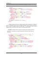
analysis {
fileanalysis { “myanalysis in.dat out.dat”,
“in.dat”, “out.dat” }
}
...
In the above case it is assumed that myanalysis is the name of the analysis program
program, file named in.dat is used as analysis input file and file out.dat is uses as analysis
output file.
If the analysis program writes its results in a different format or expect input in a
different format, then converters must be provided. If a converter is implemented as a
stand-alone program, it should be executed right after the analysis program. Since the
fileanalysis function anticipates execution of only a single system command, this can be
solved in two ways. First, if the system permits successive execution of several programs
by passing a single command (e.g. by using a semicolon or a newline for separation of
commands), then the command can be composed in the appropriate way:
“convertaninfile in.dat \n
convertanoutfile out.dat”
myanalysis in.dat out.dat
\n
where convertaninfile is the name of the program that reads the analysis input file in the
format described in Section 7.2.1 and writes it back in the format readable by the
myanalysis program, and convertanoutfile is the name of the program that reads the
analysis output file in the format used by the myanalysis program and writes the data
back to the file in the format specified in Section 7.2.2.
Below there is an example of running an external analysis program by using
converters:
...
setstring {
out.dat \n
setstring {
setstring {
ancom “convertaninfile in.dat
convertanoutfile out.dat” }
aninfile “in.dat” }
anoutfile “out.dat” }
31
\n
myanalysis in.dat
INVERSE 3.18
7.1: Uniform File Interface Between Optimization and Analysis Programs / Interpreter
functions
...
analysis {
fileanalysis { #ancom, #aninfile, #anoutfile }
}
...
7.1.1.2 fileanalysis_oneline { ancommand aninfile anoutfile < cd >
}IOptLib
The same as fileanalysis, except that input data for direct analysis is written in a
single line in the analysis input file. By specification, this should not matter for parsers of
the analysis input file.
7.1.1.3 filewriteaninput { filename < cd > }IOptLib
Writes direct analysis input data to the file named filename (string argument). The
data are obtained from the pre-defined interpreter variables: optimization parameters
from vector variable parammom and request calculation flags from counter variables
calcobj, calcconstr, calcgradobj, and calcgradconstr.
Optional string argument cd can specify additional definition data that is passed to
the direct analysis.
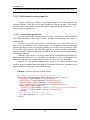
This function is usually used within the analysis block. The following interpreter
code illustrates the typical use that replaces the fileanalysis function:
analysis{
filewriteaninput {“anin.dat”, “0”}
system { “analyse anin.dat anout.dat” }
filereadanres{ “anout.dat” }
}
In this example, it is assumed that the direct analysis program is called analyse,
and it takes the input and output file as command-line arguments.
Analysis input is written to the file in the format described in Section 7.2.1.
7.1.1.4 filewriteaninput_oneline { filename < cd > }IOptLib
The same as filewriteaninput, except that the analysis input data is printed in a
single line (which is usually less readable).
32
INVERSE 3.18
7.1: Uniform File Interface Between Optimization and Analysis Programs / Interpreter
functions
7.1.1.5 filereadanres { filename }IOptLib
Reads analysis results from the analysis output file (in the standard format) named
filename (string argument). The data that are defined are stored to the corresponding
standard interpreter variables (i.e. objective function to objectivemom, constraint
functions to constraintmom, gradient of the objective function to gradobjectivemom and
constraint gradients to gradconstraintmom). Calculation flags are also stored to counter
variables calcobj, calcconstr, calcgradobj, and calcgradconstr.
The file must contain analysis results in the standard form described in Section
7.2.2.
7.1.1.6 filewriteanres { filename }IOptLib
Writes current analysis results extracted form the standard interpreter variables to
the file named filename in the format described in Section 7.2.2. filename is a string
argument.
This function is used for writing analysis results e.g. in the example described in
Section 7.4 where Inverse itself acts as analysis program. In this example, reading
analysis input is performed by the parsefilevar function (Section 7.1.1.13).
7.1.1.7 filereadaninput { filename }IOptLib
Reads analysis input (i.e. parameter values and request calculation flags) from the
file named filename. Analysis input must be written to the file in the format described in
Section 7.2.1. filename is a string argument.
This function can be used for reading input data for direct analysis when Inverse
itself acts as the direct analysis program. It can be used instead of using the function
parsefilevar (Section 7.1.1.13), such as in the example described in Section 7.4.
7.1.1.8 fileanalysis_xml { ancommand aninfile anoutfile < cd > }IOptLib
The same as fileanalysis, except that XML format is used for transferring data
(see Section 7.2.3 and description of fileanalysis).
33
INVERSE 3.18
7.1: Uniform File Interface Between Optimization and Analysis Programs / Interpreter
functions
7.1.1.9 filewriteaninput_xml { filename < cd > }IOptLib
The same as filewriteaninput, except that XML file format is used for transferring
data (see Section 7.2.3 and description of filewriteaninput).
7.1.1.10 filereadanres_xml { filename }IOptLib
The same as filereadanres, except that XML file format is used for transferring
data (see Section 7.2.3 and description of filereadanres).
7.1.1.11 filewriteanres_xml { filename }IOptLib
The same as filewriteanres, except that XML file format is used for transferring
data (see Section 7.2.3 and description of filewriteanres).
7.1.1.12 filereadaninput_xml { filename }IOptLib
The same as filereadaninput, except that XML file format is used for transferring
data (see Section 7.2.3 and description of filereadaninput).
7.1.1.13 parsefilevar { filename < type1 varspec1 > < type2 varspec2 > …
< command1 > <command2 > … }
Parses the file named filename – extracts different data from the file and stores the
data into file interpreter variables if this is specified.
The first argument filename must be the name of the file to be parsed (string
argument).
Other arguments are arranged in an arbitrary sequence of commands (string
arguments) and pairs type, varspec where type is a string argument specifying the type of
the next argument and varspec is the variable element specification that defines the
element of the file interpreter variable into which the object read from the file is stored.
Possible type specifications are:
• “scal”, “scalar” – real number, e.g. 6.02e26 or 1.55
• “count”, “scalar” – integer number, e.g. 324
• “vector”, “vec” – vector in a list format, e.g. {1.1, 1.2, 1.3}
34
INVERSE 3.18
7.1: Uniform File Interface Between Optimization and Analysis Programs / Interpreter
functions
•
•
•
“marix”, “mat” – matrix in a list format, e.g. {{1.1, 1.2}, {2.1, 2.2}}
“string”, “str” – string, which can be embedded in double quotes, e.g.
“string element”or in curly brackets, e.g. {string element}, or can be a
single word specified without the quotes or brackets, e.g. string_element
“analysispoint”, “anpt” – analysis results in the format specified in Section
7.2.2. Analysis results can not be stored in a variable because there is no
corresponding type defined, so the only variable elemet specification
stated with this type is NULL[].
Variable element specifications stated after types are usual specifications, e.g.
v[1, 2] or str[]. The corresponding elements they refer to must exist and variables must
be of the correct type. If we don’t intend to store a given object into a variable then the
variable specification should be NULL[ ].
Available commands are the following:
• stop – instructs to stop parsing the file.
• in – current position in the parsed file is moved inside the first curly
brackets
• out – current position in the parsed file is moved out of the current curly
brackets
Example:
*{ Allocation of variables for storage of the data read form the
file: }
newvector { vecvar[5] }
newmatrix { mat[] }
parsefilevarprint{ "parsed.dat",
"count", NULL[],
"scal", NULL[],
"vec", vecvar[1],
"mat", mat[],
"str", NULL[],
"str", NULL[],
"in",
"scal", NULL[],
"vec", vecvar[2],
"out",
"scal", NULL[],
"scal", NULL[],
"anpt", NULL[],
"scal", NULL[],
"stop"
35
INVERSE 3.18
7.2: Uniform File Interface Between Optimization and Analysis Programs / File Formats
}
printvector{ vecvar[1] }
printvector{ vecvar[2] }
printmatrix{mat}
exit{}
7.2 File Formats
In order to use the uniform file interface, the analysis program must be able to
read analysis input files that provide calculation flags and parameter values, and must be
able to generate the output file in a proper way, such that analysis results can be correctly
read by the optimization program Inverse. The file formats used in the uniform file
interface are provided by the free optimization library IOptLib and are therefore free
formats. They can be freely used by any other software (either commercial or free
software), without requesting prior permission or paying royalty fees.
Warning:
Because numerical quantities are transferred through text files, special care must
be taken that all significant digits are written for each numerical value. On the
contrary, accuracy is lost, which may cause numerical problems or lead to inaccurate
results.
Practically all programming languages enable writing floating point numbers to
text files with arbitrary precision. The number of digits must usually be explicitly stated,
otherwise a default number of digits is assumed, which can lead to insufficient accuracy.
In C, for example, numbers are usually written to text files by using the printf function
where format specification is given. The following format specification can be used to
preserve the floating point precision:
…
double x;
FILE *fp;
…
fprintf(fp,“%.30lg”,x);
Text that begins with the % sign represents the format specification. “.30”
specifies that 30 significant digits should be output when printing a floating point
number. A large number of digits was specified in order to make sure that no precision is
lost. Part “lg” of the specification determines that a floating point is being printed in
36
INVERSE 3.18
7.2: Uniform File Interface Between Optimization and Analysis Programs / File Formats
compact format (‘g’), and that a type “long double” is expected (‘l’). In compact format,
eventual redundant digits (i.e. digits that exceed the actual precision of the floating point
number type “long double”) are not printed.
7.2.1 File format for analysis request (analysis input file)
{ { p1, p2, … }, { reqcalcobj, reqcalcconstr, reqcalcgradobj,
reqcalcgradconstr }, cd }
Meaning of symbols used above is as follows
p1, p1, p3 – optimization parameters at which analysis was performed
Flags that tell whether something has actually been calculated (0 – yes, 1- no):
• reqcalcobj – flag for the objective function
• reqcalcconstr – flag for constraint functions
• reqcalcgradobj – gradient of the objective function
• reqcalcgradconstr – gradients of constraint functions
cd – a free parameter that can be used to transfer additional information to the
direct analysis. In principle cd can be anything embedded in curly brackets ({..}) If only
the eventual embedded curly brackets are properly closed. Most commonly it will not be
used at all and therefore empty brackets (“{}”) will be put in place of cd. Otherwise,
interpretation of what stands in curly bracket is entirely in the domain of the analysis
program, therefore the documentation of the analysis program should provide information
on how to compose cd.
7.2.2 File format for analysis results (analysis output file)
{
{ p1, p2 ... },
{
calcobj, obj,
calcconstr, { constr1, constr2, ... },
calcgradobj, { dobjdp1, dobjdp2, ... },
calcgradconstr,
{
{ dconstr1dp1, dconstr1dp2, ... },
{ dconstr2dp1, dconstr2dp2, ... },
...
},
errorcode
},
37
INVERSE 3.18
7.2: Uniform File Interface Between Optimization and Analysis Programs / File Formats
{ reqcalcobj, reqcalcconstr, reqcalcgradobj, reqcalcgradconstr }
< , { ind1, ind2, ... }, { coef1, coef2, ... }, defdata >
}
Meaning of symbols used above is as follows
p1, p1, p3 – optimization parameters at which analysis was performed. These are
input data for a direct analysis, but it is requested that they are included in the output file;
in this way the optimization program can verify that the analysis results refer to the
expected set of parameters, or verify what errors were perpetrate by transfer via text
files.
Flags that tell whether something has actually been calculated (0 – yes, 1- no):
• calcobj – flag for the objective function
• calcconstr – flag for constraint functions
• calcgradobj – gradient of the objective function
• calcgradconstr – gradients of constraint functions
obj – value of the objective functions
constr1, constr2, … - values of the constraint functions
dobjdp1, dobjdp2, ... – derivatives of the objective function with respect to
individual parameters (components of the objective function gradient)
dconstr1dp1, …, dconstr2dp1, dconstr2dp2 – derivatives of individual constraint
functions with respect to individual optimization parameters – components of gradients of
the constraint functions (e.g. dconstr2dp3 is the derivative of the second constraint
function with respect to the third parameter)
errorcode – integer error code of analysis – 0 for no error, usually a negative
number for errors, values are function specific
reqcalcob , reqcalcconstr, reqcalcgradobj and reqcalcgradconstr are request
flags for calculation of the various values, as have been passed to the analysis function.
The same as with parameter values, these flags are requested only for verification. In vast
majority of cases these flags will not be used by the optimization program, and they can
simply be set to 1.
Angle brackets < ... > contains portion of data that is optional and can be omitted
(in the file, there are no angle brackets).
ind1, ind2, … is a set of integer numbers that can be used to pass some
supplemental data about a particular calculation (e.g. the sequential number of the
particular analysis that the analysis server performed). In most cases the set will be
empty, i.e. {}
coef1, coef2, … is a set of real numbers that can be used to pass some data about a
particular calculation. In most cases the set will be empty, i.e. {}
cd is the definition data for the analysis. It can have different forms, usually it is
an integer and does not have any meaning.
Spaces, tab characters and newlines are not important. Empty brackets should be
used for any vector or set of vectors that are not calculated.
38
INVERSE 3.18
7.2: Uniform File Interface Between Optimization and Analysis Programs / File Formats
Examples:
{ {1.11, 2.22}, { 1, 6.1605, 1, {-0.165, -2.44} , 1, {2.22, 4.44},
1, { {-1.5, 0.}, {0., -2.} }, 0 }, { 1, 1, 1, 1}, {}, {}, "3" } }
{ {1.11, 2.22}, { 1, 6.1605, 1, {-0.165, -2.44} , 0, { }, 0, {
-1 }, { 1, 1, 1, 1}, {33, 45}, {2.5, 3.33 38.1}, "3" } }
},
The examples represent analysis results at parameters {1.11, 2.22}, with value of
the objective function 6.1605, values of constraint functions -0.165 and -2.44, gradients
of the objective function {2.22, 4.44}, gradient of the first constraint function {-1.5, 0.},
and gradient of the second constraint function {0., -2.}.
In the second example, gradients of the objective and constraint functions could
not be calculated although they were requested (all request calculation flags in curly
brackets are 1). Therefore, the error code is -1 rather than 0.
7.2.3 XML formats
7.2.3.1 XML format for analysis results (analysis output file):
Example 1 shows an example of the analysis output file in XML format. The
structure of the file can be easily established form this example, and precise rules are
stated below.
7.2.3.1.1 Format rules (general)
Comments are ignored when processing the analysis output file, and all of them
can be omitted. Comments can only be put before XML elements (they may not be put
within opening or closing tags).
Name of the outer-most element is arbitrary, but “data” is recommended. All
other names must be precisely as in the example.
Names of attributes of individual XML elements with specific meaning must
exactly match names from the example, and XML elements with specific meaning must
have all the attributes defined as in the example. Order of attributes is not important, but
attribute names must be unique for a given element. Values of attributes must also match
exactly, except for those attributes that specify dimensions or indices. Such attributes are
only dim (which specifies the dimension – or number of elements – of given data) and ind
(which specify the index of component – sub-element – of given data). Values of such
attributes must be strings that represent integer numbers in base 10 notation.
39
INVERSE 3.18
7.2: Uniform File Interface Between Optimization and Analysis Programs / File Formats
Each data element has the attribute type defined, which specifies the type of the
data represented by the XML element. Types used in the analysis output file are counter
(representing an integer number), scalar (representing a real number), vector
(representing a real vector), string (representing a string of characters), table
(representing a table of elements of any kind, all elements of the same kind) and
analysispoint (representing a structure that carries analysis input and/or output data).
Elements of type counter (i.e. those whose attribute type has value counter) must
have contents that can be interpreted as an integer, e.g. “1”, “425”, “-10”, etc.
Elements of type scalar must have contents that can be interpreted as a real
number, e.g. “06”, “1.45”, “-10.4e-5”, etc.
Elements of type vector must have an attribute named dim, whose value must be a
string representation of vector dimension (e.g. “12” if the vector is of dimension 12). All
components of the vector must be listed as sub-elements of type scalar, with element
names “vector_el”. Beside the attribute “type” (whose value must be “scalar”), these
elements must have the attribute “ind”, which must be a string representation of an
integer that is equal to the index of specific vector component.
Elements of type table must have an attribute named dim, whose value must be a
string representation of the number of elements of the table (e.g. “5” if the table has 5
elements). Element of type table must have the attribute named eltype, whise value must
be equal to the type of the table elements. All components of the table must be listed as
sub-elements of a given type (arbitrary but the same for all elements of the table, and the
type must match the value of the eltype attribute of the table element), with element
names “table_el”. Beside the attribute “type”, these elements must have the attribute
“ind”, which must be a string representation of an integer that is equal to the index of
specific table element.
Sub-elements of the element whose type is analysispoint can be omitted if they
are not relevant. For example, if the gradient of the objective function has not been
calculated then the element named gradobjective can be omitted.
The order in which sub-elements are listed is not important.
7.2.3.1.2 Analysis output-specific rules
The above stated rules are general, while the following additional rules apply for
the analysis output file:
The outer-most XML element must be of type “analysispoint” and its attribute
named mode must have value “analysis_output”.
Element ret of type counter must be defined. It must have the integer value 0 if no
errors were detected in the analysis, or a negative integer value if errors occurred.
Elements reqcalcobj, reqcalcconstr, reqcalcgradobj and reqcalcgradconstr of
type counter may be omitted. If included then their values must be 1 if calculation of the
corresponding portions of analysis results were requested (actually, any non-zero value is
allowed), and 0 if not. They correspond to the following portions of analysis results,
40
INVERSE 3.18
7.2: Uniform File Interface Between Optimization and Analysis Programs / File Formats
respectively: objective function, constraint functions, gradient of the objective function
and gradients of constraint functions.
Elements calcobj, calcconstr, calcgradobj and calcgradconstr of type counter are
obligatory. Their values must be 1 if calculation of the corresponding portions of analysis
results were requested (actually, any non-zero value is allowed), and 0 if not. They
correspond to the following portions of analysis results, respectively: objective function,
constraint functions, gradient of the objective function and gradients of constraint
functions.
Element param of type vector must contain values of optimization parameters for
which analysis results were calculated. In Example 1, vector of parameters has dimension
2 and therefore 2 sub-elements of type scalar that carry its components.
Element obj of type scalar contains (if defined) the value of the objective
function.
Element constr of type table contains (if defined) the values of the constraint
functions. It must have as many sub-elements as there are constraints. Its elements must
be of type scalar and must carry values of individual constraints.
Element gradobj of type vector contains (if defined) the gradient of the objective
function. It must have as many sub-elements as the number of parameters.
Element gradconstr of type table contains (if defined) gradients of the constraint
functions. It must have as many sub-elements as there are constraints. Sub-elements must
be of type vector and their dimension must he equal to the number of parameters.
Element cd is an optional element of type string. It can contain additional data
(such as analysis definition data) that might be exchanged between the optimization and
analysis routines. In many cases, this field is not used.
Example 1: Analysis output file in XML format (2 parameters, 2 conatraints, all
values and gradients calculated).
<!-- Analysis output file, created by analysis wrapper. -->
<data type="analysispoint" mode="analysis_output" ind="1">
<ret type="counter">0</ret>
<reqcalcobj type="counter">1</reqcalcobj>
<reqcalcconstr type="counter">1</reqcalcconstr>
<reqcalcgradobj type="counter">1</reqcalcgradobj>
<reqcalcgradconstr type="counter">1</reqcalcgradconstr>
<calcobj type="counter">1</calcobj>
<calcconstr type="counter">1</calcconstr>
<calcgradobj type="counter">1</calcgradobj>
<calcgradconstr type="counter">1</calcgradconstr>
<param type="vector" dim="2">
<vector_el type="scalar" ind="1">1.6</vector_el>
<vector_el type="scalar" ind="2">1</vector_el>
</param>
<obj type="scalar">0.20088905308774715</obj>
<constr type="table" eltype="scalar" dim="2">
<table_el type="scalar" ind="1">0.0</table_el>
<table_el type="scalar" ind="2">0.0</table_el>
41
INVERSE 3.18
7.2: Uniform File Interface Between Optimization and Analysis Programs / File Formats
</constr>
<gradobj type="vector" dim="2">
<vector_el type="scalar" ind="1">0.24138</vector_el>
<vector_el type="scalar" ind="2">0.0172418</vector_el>
</gradobj>
<gradconstr type="table" eltype="vector" dim="2">
<table_el type="vector" dim="2" ind="1">
<vector_el type="scalar" ind="1">-1.1</vector_el>
<vector_el type="scalar" ind="2">2.1</vector_el>
</table_el>
<table_el type="vector" dim="2" ind="2">
<vector_el type="scalar" ind="1">0</vector_el>
<vector_el type="scalar" ind="2">-1</vector_el>
</table_el>
</gradconstr>
<!-— Optional definition data: -->
<cd type="string">Definition data</cd>
</data>
Another example below shows another possible analysis output file, in which the
values of calculation requests flags are skipped, gradients are not calculated (obviously
they were also not requested since the return value is 0, indicating no errors), and no
additional data is passed between the analysis and optimization module.
Example 2: Another analysis output file with only partial output provided (3
parameters, 2 constraint, no gradients requested or calculated, request flags not
specified).
<!-- Analysis output file, created by analysis wrapper. -->
<data type="analysispoint" mode="analysis_output" ind="1">
<ret type="counter">0</ret>
<calcobj type="counter">1</calcobj>
<calcconstr type="counter">1</calcconstr>
<calcgradobj type="counter">0</calcgradobj>
<calcgradconstr type="counter">0</calcgradconstr>
<param type="vector" dim="3">
<vector_el type="scalar" ind="1">4.287974793</vector_el>
<vector_el type="scalar" ind="2">105.38479</vector_el>
<vector_el type="scalar" ind="3">2.4558e-4</vector_el>
</param>
<obj type="scalar">72.424979429783</obj>
<constr type="table" eltype="scalar" dim="2">
<table_el type="scalar" ind="1">-1.48479e-3</table_el>
<table_el type="scalar" ind="2">2.8793872</table_el>
</constr>
</data>
42
INVERSE 3.18
7.2: Uniform File Interface Between Optimization and Analysis Programs / File Formats
7.2.3.2 XML format for analysis input file
Example 3 shows an example of the analysis input file in XML format. The
complete structure of the file can be easily established form this example. The general
rules are similar to the general rules for the analysis output file stated in Section 7.2.3.1.1.
Specific rules are stated below.
7.2.3.2.1 Analysis input-specific rules
The outer-most XML element must be of type “analysispoint” and its attribute
named mode must have value “analysis_input”. Its name can be arbitrary, but “data” is
recommended.
Elements reqcalcobj, reqcalcconstr, reqcalcgradobj and reqcalcgradconstr of
type counter are obligatory.Their values must be 1 if calculation of the corresponding
portions of analysis results are requested (actually, any non-zero value is allowed), and 0
if not. They correspond to the following portions of analysis results, respectively:
objective function, constraint functions, gradient of the objective function and gradients
of constraint functions.
Element param of type vector must contain values of optimization parameters for
which analysis results are to be calculated. In Example 3, vector of parameters has
dimension 2 and therefore 2 sub-elements of type scalar that carry its components.
Element cd is an optional element of type string. It can contain additional data
(such as analysis definition data) that might be exchanged between the optimization and
analysis routines. In most cases, this field is not used.
Example 3: Analysis input file in XML format.
<!— Analysis input file, created by IOptLib. -->
<data type="analysispoint" mode="analysis_input" ind="1">
<reqcalcobj type="counter">1</reqcalcobj>
<reqcalcconstr type="counter">1</reqcalcconstr>
<reqcalcgradobj type="counter">1</reqcalcgradobj>
<reqcalcgradconstr type="counter">1</reqcalcgradconstr>
<param type="vector" dim="2">
<vector_el type="scalar" ind="1">1.6000000000000001</vector_el>
<vector_el type="scalar" ind="2">1</vector_el>
</param>
<!-— Optional definition data: -->
<cd type="string">Definition data</cd>
</data>
43
INVERSE 3.18
7.3: Uniform File Interface Between Optimization and Analysis Programs / Solution
Scheme
7.2.3.3 XML format for storage of analysis results (“analysis point”):
7.3 Solution Scheme
Integrated environment:
Prepare FEM analysis
Run analysis
Define optimization parameters
Run optimization
Inverse input
fiele(s)
Additional data file(s):
These data define precisely
how to perform analysis
opt.cm
Inverse (optimization program):
Run optimization
Inside optimization loop (iteratively):
• write {α, d} to a file
• run Analysis program
• read f({α, d}) from a file
anin.dat
invanan.cm
Analysis input
file
{{p}, …}
Analysis program:
Output results
Analysis output
file
f, ci , ...
anout.dat
read {α, d} from a file
prepare FEM input
run FEM prog.
read results
calculate f(p), ci(p)
write f, ci to a file
FEM input
file
FEM analysis:
read input
perform analysis
output results
FEM output
file
Figure 1: Typical software organization when using uniform file interface
between optimization and analysis module (which are implemented as stand-alone
programs). Analysis module is a program that reads parameters and calculation flags
from analysis input file, performs direct analysis (i.e. calculates the objective and
constraint functions and eventually their gradients) and outputs these results to the
analysis output file (response file). In the scheme, {α, d} denote optimization
parameters, f is objective function and ci constraint functions. Solid arrows denote
44
INVERSE 3.18
7.4: Uniform File Interface Between Optimization and Analysis Programs / Demonstrative
example
data flow and dotted arrows denote calling directions. Horizontal arrows denote
calling directions that are commonly present. Other calls are performed when the
optimization and simulation modules are integrated in a broader framework.
7.4 Demonstrative example
An example has been set up in order to demonstrate use of the uniform file
interface. The example files are contained in the directory named filean in
IGHOME/inverse/ex.
An example contains a synthetic case for which analytical response functions are
defined. There are two optimization parameters and two constraints. Both optimization
and direct analysis are performed by Inverse with appropriate command files defined
separately for optimization and analysis. Usually this will not be the case and there will
be a separate program for the direct analysis, such as in Figure 1 where a special analysis
program runs a finite element simulation and calculates the response function.
7.4.1 List of files
The main files are the following:
opt.cm - command file for optimization (performed by Inverse)
an.cm - command file for direct analysis (also performed by Inverse)
anin.dat - analysis input file (written by optimization program and read by
analysis program), contains current values optimization parameters, calculation request
flags and possibly an additional analysis definition data (Section 7.2.1)
anout.dat – analysis output file (written by analysis program and read by
optimization program), contains analysis results (response functions such as objective and
constraint functions and their gradients, and calculation flags – see Section 7.2.2).
Auxiliary files:
def.cm – command file that contains some basic definitions and initialization
steps. Its interpreted both from an.cm and opt.cm since these definitions are used
commonly by the optimization and analysis program.
defuser.cm – additional definitions. This file is included in def.cm via the
interpret{} command. Location of inclusion is such that important definitions from def.c
are overridden, but dependent portion of the definitions (such as allocation of the
45
INVERSE 3.18
7.4: Uniform File Interface Between Optimization and Analysis Programs / Demonstrative
example
meaningful variables) are performed after interpretation of this file such that correct
effects are ensured. This file is convenient for automatic generation by the environment
that manipulates the analysis and optimization programs.
analysis.cm - additional command file for analysis program, contains definitions
of functions for calculating the response and definition of analysis block. It is interpreted
form an.cm.
Control files:
opt.ct – control file for optimization program, here the optimization program
writes its results if this is ordered in its command file. The file can be used for checking
the course of execution.
an.ct – control file for analysis program.
Control files should be deleted from time to time because output is appended to existent
contents, so that output from several successive runs can be checked.
Sample analysis program:
analysis.c – a C language source for a sample analysis program. A function for
reading the analysis input data in standard format (Section 7.2.1) and for writing analysis
results in the standard format (Section 7.2.2). The program uses only standard C libraries
and ANSI C syntax, therefore it can be easily compiled on any platform provided that a C
7.4.2 Running the example and using custom analysis program
In order to run the example, optimization program Inverse must be installed on
your computer. Let’s assume that invan is the command for executing Inverse. Then the
example is run by typing the following command in the operating system’s command
shell:
invan opt.cm
Main definitions that one may want to change in order to modify the example (i.e.
to modfy the optimization method used or the definition of the problem / response
functions) are in the file def.cm. By setting e.g. the calculator variable unconstrained to 1,
the unconstrained simplex method is used instead of the constraint method, and penalty
terms are added to the constraint functions in order to prevent constraint violations.
Definitions in the file are commented (comments are inside *{…}), such that their
meaning is obvious to the user.
The file defuser.cm is included in def.cm. Definitions that should override the
definitions in
46
INVERSE 3.18
7.4: Uniform File Interface Between Optimization and Analysis Programs / Demonstrative
example
7.4.3 Using a different analysis program
Example can be easily re-arranged in order to use a different analysis program.
In the file def.cm, the string variable ancommand must be modified such that it contains
the command that runs that analysis program, e.g.
setstring{ ancommand "my_analysis inputfile outputfie" }
if the analysis program is run by command my_analysis with arguments inputfile and
outputfile that define its input and output file. In this case, inputfile and outputfile must be
names of the files that are specified in def.cm as analysis input and analysis output file,
and these are contained in the string variables aninfile and anoutfile defined in def.cm.
Another possibility is that the analysis program uses input and output files with
pre-defined names that are always the same, or that names of these files are defined in
some kind of resources file. It is only important that the files are synchronized between
the optimization and the analysis program, therefore names of the analysis input and
output files must be updated accordingly for the optimization program, which is done
simply by appropriately setting the string variables aninfile and anoutfile in the definition
file def.cm.
Beside re-defining the command for running the analysis program and taking care
that the optimization program and analysis program use the same analysis input and
analysis output file, some variables related to the optimization problem definition must be
updated accordingly. In def.cm, calculator variable numparam must be set to actual
number of optimization parameters in the problem that is actually defined by the analysis
program, and numconstr must be set to the actual number of constraints for the new
problem. Dimensions of some other relevant variables that depend on these numbers are
set automatically in def.cm.
Then, commands in opt.cm that perform the optimization must be modified such
that their arguments are consistent with the specific optimization problem that is solved
and defined by the external analysis program. Such commands are inverse and optfsqp. In
particular, the dimensions of the starting guess must be corrected and arguments that are
dependent or define the number of optimization parameters or the number of constraints.
Legend:
IOptLib :
47
INVERSE 3.18
7.4: Uniform File Interface Between Optimization and Analysis Programs / Demonstrative
example
This
functionality
is
Optimization Library)[2].
from
IOptLib
(Investigative
References:
[1]
I. Grešovnik, Simplex Algorithms for Nonlinear Constraint Optimization
Problems, revision 0, technical report, 2007.
[2]
I. Grešovnik, IoptLib User's Manual,, revision 0, library manual, 2007.
48