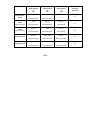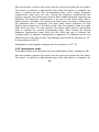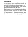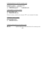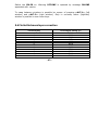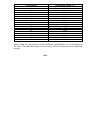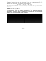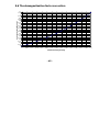
1
Magnetic susceptibility meter
SM-30
USER’S MANUAL
Publications Date: June 2003
Terraplus USA Inc.
1.GENERAL INFORMATION .................................................... 4
1.1 Application .........................................................................4
1.2 Specification .......................................................................5
2. DESCRIPTION OF INSTRUMENT ......................................... 6
2.1 General description ..............................................................6
2.2 Operating principles .............................................................7
2.2.1
2.2.2
2.2.3
2.2.4
2.2.5
2.2.6
Basic modes A and B....................................................................... 8
Extrapolation mode ........................................................................ 9
Interpolation mode....................................................................... 10
Scanning mode ............................................................................. 10
Averaging mode ........................................................................... 11
Comparison of modes ................................................................... 11
3. OPERATION..................................................................... 14
3.1 Switching instrument ON and OFF ........................................14
3.2 Setting and indication of mode ............................................15
-1-
3.3 Measuring susceptibility of rock ...........................................15
3.3.1
3.3.2
3.3.3
3.3.4
3.3.5
Basic modes A, B .......................................................................... 15
Extrapolation mode ...................................................................... 16
Interpolation mode....................................................................... 17
Scanning mode ............................................................................. 19
Averaging mode ........................................................................... 21
3.4 Memory registers...............................................................22
3.5 Battery replacement...........................................................24
3.6 Communication with computer.............................................25
3.6.1 General information ..................................................................... 25
3.6.2 Instrument operation using computer.......................................... 25
3.6.3 Transfer of data to computer........................................................ 26
3.7 Error messages .................................................................28
4 FIGURES .......................................................................... 30
4.1
4.2
4.3
4.4
4.5
Figure 1 ...........................................................................30
Figure 2 ...........................................................................31
Figure 3 ...........................................................................32
Figure 4 ...........................................................................33
Figure 5 ...........................................................................34
-2-
4.6 Figure 6 ...........................................................................35
4.7 Figure 7 ...........................................................................36
5.APPENDICES .................................................................... 37
5.1 SM30 software ..................................................................37
5.2 SM30 programme for Windows 95/98/NT/2000 ......................37
5.2.1
5.2.2
5.2.3
5.2.4
5.2.5
Running the program.................................................................... 37
Reading memory registers............................................................38
Communicating with the computer on-line ................................... 38
Handling the charts ...................................................................... 39
Saving the data ............................................................................ 40
5.3 SM30 programme for DOS ..................................................41
5.4 Finite thickness layer correction ...........................................42
5.5 Conductivity effect .............................................................44
5.6 The demagnetisation factor correction ..................................45
-3-
1.GENERAL INFORMATION
1.1 Application
The SM-30 meter is intended for measuring the magnetic susceptibility of rock.
Owing to its high sensitivity, it is capable of measuring rock with a very low
susceptibility. It can also measure diamagnetic substances. The meter reaches its
peak sensitivity within a very few seconds after switch-on. By employing a very
sophisticated way of processing the signal, the meter can efficiently reduce the
influence of external electromagnetic disturbances and the noise of electronic
circuits. Its low weight and small size make this instrument ideal for use
out-of-doors.
-4-
1.2 Specification
SENSITIVITY……………………………………………………………………………………..x10-7 SI Units
MAX MEASURED VALUE………………………………………………………………………………….10-1SI
DIMENSIONS……………………………………………………………….……………..100 x 65 x 25 mm
WEIGHT………………………………………………………………………………………….……………0.180 kg
OPERATING FREQUENCY………………………………………………………………………………..…9kHz
MEASUREMENT TIME
• …………………………………………………………………………………….basic mode approx. 5s
• …………………………………………………………………..drift correction modes approx. 8s
DIGITAL DISPLAY………………………………………………………………….LCD 4digit,10mm high
CONTROLS…………………………………………………………………………………………3 push buttons
DATA MEMORY………………………………………………………………….up to 250 measurements
PICK-UP COIL SIZE 50 mm in diameter
OPERATING TEMPERATURE……………………………………………………………..-20o C to +50 oC
BATTERY……………………………………………………………….….…….2 Lithium 3V type CR2430
BATTERY LIFE…………………………………………………………….………………..typically 80 hours
COMMUNICATION WITH COMPUTER……………………………………………………………..RS232
-5-
2. DESCRIPTION OF INSTRUMENT
2.1 General description
The susceptibility meter is enclosed in a box, which has a front panel with push
buttons and a four-digit 10mm character display. In order to get the right value
in SI, the user must multiply the reading by a constant 10-3 .
Behind the front panel there is a buzzer, which monitors by way of acoustics the
operation of the meter. On the right-hand side of the cover there is a connector
for communication with a computer. A communication cable is delivered as part
of the set. On the bottom side of the cover there is a little cubicle holding two Li
batteries.
The 50mm pickup coil is placed on the left-hand side parallel with the bottom
part of the cover (see figure 6).
-6-
2.2 Operating principles
The meter contains an oscillator with a pickup coil. The frequency of the oscillator
depends on the distance of the meter from rock. the change in frequency is
proportional to the amount of suceptibility of the rock. In order to find out about
the change, it is necesary to measure the oscillator frequency twice. The first
measurement is performed near the rock. This is called pick-up step.
The second measurement is carried out when the meter is away from the rock
(free air measurement). The second phase is called compensation step.
After the second step is finished, both values are subtracted and displayed. Both
the steps are initiated by the operator.
The above mentioned mode is called basic mode or mode 1.
When measuring rock of very low susceptibility, it is possible that the oscillator
thermal drift becomes greater than the effect of the rock. In this case it is
necessary to measure not only the susceptibility, but also the thermal drift. The
thermal drift and susceptibility values are then compared. The thermal drift
measurement requires that two measurements away from rock are carried out,
which means that there have to be three steps altogether. Two steps are
performed without rock and one is performed with rock. The SM-30 meter offers
two ways of correcting the dirft. The first mode is called extrapolation mode or
mode 2.
-7-
The second mode is called interpolation mode or mode 3.
When measuring places that are situated very close to one another, it is best to
use scanning mode.
This mode corrects the thermal drift as well and the measurement is very quick,
although the drift correction is not so precise as in the extrapolation or
interpolation mode.
2.2.1 Basic modes A and B
The function of the meter is shown in Figure 1a. Figure 1b shows the way the
oscillator frequency is affected by the measured object. It also shows the
frequency difference in both the steps. The difference is used as ground for the
calculation of magnetic susceptibility. Figure 1 deals with an ideal case, when
there is no thermal drift. Susceptibility is calculated using the formula
susc = f 2 - f1
After the compensation step is finished, the value
susc is displayed.
Figure 2 shows the effects of thermal dirft during Basic mode. It shows that the
oscilaltor frequency is not only influenced by the measured rock during the
pickup step, but it changes without any apparent reason and casues
measurement error.
-8-
The SM-30 has two basic modes A and B. The only difference between modes A
and B is in the length of the pick-up and compensation steps. The basice mode B
has these steps 4 times faster than mode A. Mode B is suitable for measuring
medium and high susceptibility.
2.2.2 Extrapolation mode
Thermal drift correction is described in Figure 3. The time elapsed during the
pickup step and the first compensation step depends on the operator. The time
lag between the second and first compensation steps is set automatically and it is
t as well. It is then quite easy to measure the value of drift.
drift = f 3 - f2
It is valid that
susc + drift = f 2 - f1
Furthermore
susc = f 2 - f1 - (f3 - f2) = 2f 2 - f1 - f3
-9-
The corection of drift is performed automatically according to the last equation.
After the first compensation step is finished, the display shows first the
uncorrected f2 - f1 value. After the second compensation step is finished, the
value is corrected and the display shows the value 2f2 - f1 - f3.
2.2.3 Interpolation mode
This method requires that the user put the meter near rock during the second
step. The first and third steps are compensation steps. The third step of this
mode (the second compensation step) is initiated automatically. Figure 4 makes
it possible to derive
susc = (f1 + f3)/2 - f2 = -1/2 (2f2 - f1 -f3)
The reading is corrected after the second compensation step and the display
shows the value -1/2 (2f2 - f1 - f3).
2.2.4 Scanning mode
The principle is clear from Figure 5, which shows the block of measurement. The
first and last steps are compensation (free air). The first compensation step is
initiated by the left button. Afterwards come pickup steps (near the rock), which
are started by the left button as well. The measurement is finished with the
second compensation steps, initiated by the middle button. The display shows
- 10 -
after each pickup step the susceptibility value, calculated similar to the Basic
mode. This calculation takes into consideration the value measured during the
first compensation step fc1. The susceptibility is stored in the operation memory
of the processor together with the time elapsed since the first compensation step
(see Figure 5). After performing the second - final - compensation step (middle
button), drift correction is made using interpolation. The corrected susceptibility
values are stored in memory registers to be displayed in the ususal manner.
The total number of pickup steps in one block is 20. After the 20th pick-up step
the instrument warns the operator that measured block has to be terminated by
second compensation step.
2.2.5 Averaging mode
This mode is very similar to Scanning mode (mode 4). The only difference is in
the very end of measuring procedure. After the middle button is pressed and
drift correction is done, the average value is calculated and put into memory
register (see Figure 5).
2.2.6 Comparison of modes
Both basic modes are simple and yet applicable in most situations. Basic mode B
is suitable for medium and high susceptibility. Extrapolation mode is useful when
measuring low susceptibility rock. The operation of the meter is the same as
during the Basic mode, only the correction of the final value takes a few seconds
longer.
- 11 -
The advantages of the interpolation method can be seen in the equations in 2.2.2
and 2.2.3. A comparison of both calculations shows that the Interpolation mode
requires the result to be divided by -2. This means that the value is twice as
precise as with the extrapolation method. The correct value is obtained by
processing the data in the same way as with extrapolation method and dividing it
by -2.
The interpolation method offers twice as effective noise reduction as the
extrapolation method. It is, however, less similar to the basic modes used in
most measurements.
The interpolation method is useful when dealing with samples of very low
susceptibility.
The scanning mode is best in such cases as measuring a number of points on a
profile. Core is a good example. In order to measure n values it is necessary to
measure the frequency n+2 times, while during extrapolation or interpolation
method it is necessary to perform 3n measurements.
The disadvantage of the scanning mode lies in the lesser ability to reduce drift.
This is especially the case when the number of pickup steps between two
compensation steps is too high.
Due to the lower reduction of drift, the readings are displayed with the definition
of 10-6 SI.
The following table makes it possible to compare the six usual modes.
- 12 -
basic modes
A&B
*)
extrapolation
mode
(drift correction)
interpolation
mode
(drift correction)
object
measurement
&
init.
object
measurement
&
init.
rock
free air
object
measurement
&
init.
resolution
[SI Units]
- - -- - - -- -
press left button
press left button
rock
free air
free air
press left button
press left button
automatically
free air
rock
free air
10-6
10-7
10
press left button
press leftt button
automatically
free air
rock n-times
free air
press left button
press left button
press right button
free air
rock n -times
free air
press left button
press left button
press right button
scanning mode
averaging mode
*) Basic mode B has 4 times faster measuring time than basic mode A.
- 13 -
-7
10-6
10-7
3. OPERATION
3.1 Switching instrument ON and OFF
The meter is switched on by pressing the middle button. The meter displays
within 0.2 seconds of switchon the mode number used before the meter was
switched off. After the button is released, the last suscpetibility value is displayed
and the buzzer gives a short beep. The modes are numbered as follows:
basic mode A…...........…………………………………………………………..…….………….……..…-1-extrapolation mode………………………………………………………………………………………..…..-2-interpolation mode…….………………………………………………………..………………………….….-3-scanning mode…………………………………………………………………………………………..........-4-averaging mode….……………………………………………………………………………………..........-5-basic mode B.............…………………………………………………………...…….…….….……..…-6-The respective modes are given the same numbers during the setting up of
modes (see next chapter).
The meter is switched off by pressing the left button and holding it until the
buzzer gives a short beep to indicate switchoff. The time is approximately
5 seconds. The meter also displays the word OFF. After the button is released,
the display goes off and the meter is off as well.
- 14 -
The meter switches itself off after no button has been pressed for three minutes.
The meter gives a beep to indicate switchoff.
3.2 Setting and indication of mode
By pressing the right button first and then pressing the left button without
releasing the right one the user can display the number of mode according to the
table in the previos chapter. By pressing the left button a second time, the user
sets up a mode with a number greater by 1. Mode 4 is followed by mode 1. After
finishing this procedure, the set mode is used.
3.3 Measuring susceptibility of rock
3.3.1 Basic modes A, B
If necessary, switch the instrument into the Basic mode indicated by –1-- or by
–6--. The only difference between modes A and B is in the length of the pick-up
and compensation steps. The basice mode B has these steps 4 times faster than
mode A.
The switched on meter is put near the rock and the operator presses the left
button. The meter gives a high-pitched beep and when the operator releases the
button, the meter is performing the pickup step, or measuring frequency near
rock. During the frequency measurement the buzzer is giving a low-pitched beep.
The display shows the middle three horizontal segments. The pickup step takes
- 15 -
approximately 2 seconds. After the pickup step is finished, the buzzer goes silent
and the number of the memory register prepared to store the value is displayed.
Now the operator removes the meter from the rock and presses the left button.
The buzzer is emitting a high-pitched beep. After the button is released, the
meter is performing the compensating step, which means - in this case - one
measurement away from the rock. During the frequency measurement the
buz zer is giving a low-pitched beep and the three middle horizontal segments are
displayed. The compensating step is as long as the pickup step, that is 2
seconds. The buzzer goes silent when this step is finished and the value of
magnetic susceptibility is displayed. The displayed value must be multiplied by
10-3 to be according to the SI.
Basic mode displays readings with the resolution of 10-6 SI.
3.3.2 Extrapolation mode
If necessary, switch the instrument into the Extrapolation mode indicated by -2-The switched on meter is put near the rock and the operator presses the left
button. The meter gives a high-pitched beep and when the operator releases the
button, the meter is performing the pickup step, or measuring frequency near
rock. During the frequency measurement the buzzer is giving a low-pitched beep.
The display shows the middle three horizontal segments. The pickup step takes
approximately 2 seconds. After the pickup step is finished, the buzzer goes silent
and the number of the memory register prepared to store value is displayed.
- 16 -
Now the operator removes the meter from the rock and presses the left button.
The buzzer is emitting a high-pitched beep. After the button is released, the
meter is performing the first compensating step, which means frequency
measurement away from the rock. During the frequency measurement the
buzzer is giving a low-pitched beep and the three middle horizontal segments are
displayed. The frequency measurement is as long as the pickup step, that is
approximately 2 seconds. The buzzer goes silent when this step is finished and
the measured value is displayed. The same value would constitute the final
reading when measuring in the Basic mode. Now the operator holds the meter
away from the rock. In a few seconds, the buzzer starts giving a low-pitched
beep to indicate the second compensating step, which means the second
frequency measurement away from the rock. After the step is finished, the
corrected value of magnetic susceptibility is displayed. The obtained value is not
affected by the linear part of drift. The displayed value must be multiplied by 10-3
to be according to the SI.
Extrapolation mode displays readings with the resolution of 10-7 SI.
3.3.3 Interpolation mode
If necessary,switch the instrument into the Interpolation mode, indicated by -3-Now the operator removes the meter from the rock and presses the left button.
The buzzer is emitting a high-pitched beep. After the button is released, the
- 17 -
meter is performing the first compensating step, which means frequency
measurement away from the rock. During the frequency measurement the
buzzer is giving a low-pitched beep and the three middle horizontal segments are
displayed. The first compensating step is approximately 2 seconds long. The
buzzer goes silent when this step is finished and the number of the memory
register prepared to store value is displayed.
The meter is now put near the rock and the operator presses the left button
again. The buzzer gives a high-pitched beep and when the operator releases the
button, the meter is performing the pickup step, or measuring frequency near
the rock. During the frequency measurement the buzzer is giving a low-pitched
beep. The display shows the middle three horizontal segments. The pickup step is
as long as the first compensating step, that is approximately 2 seconds. After the
frequency measurement is finished, the buzzer goes silent and the measured
value is displayed. The same value would constitute the final reading when
measuring in the Basic mode. Now the operator holds the meter away from the
rock. In a few seconds, the buzzer starts giving a low-pitched beep to indicate
the second compensating step, which means the second frequency measurement
away from the rock. After the step is finished, the corrected value of magnetic
susceptibility is displayed. The obtained value is not affected by the linear part of
drift. The result must be multiplied by 10-3 to be in the SI units. Interpolation
mode displays readings with the resolution of 10-7 SI.
- 18 -
3.3.4 Scanning mode
If necessary, switch the instrument into the Scanning mode, indicated by -4-The operator removes the meter from the rock and presses the left button. The
buzzer is emitting a high-pitched beep. After the button is released, the meter is
performing the first compensating step, which means frequency measurement
away from the rock. During the frequency measurement the buzzer is giving
a low-pitched beep and the three middle horizontal segments are displayed. The
first compensating step is approximately 2 seconds long. The buzzer goes silent
when this step is finished and the number .0000 is displayed.
The meter is now put near the rock and the operator presses the left button
again. The buzzer gives a high-pitched beep and when the operator releases the
button, the meter is performing the pickup step, or measuring frequency near
the rock. During the frequency measurement the buzzer is giving a low-pitched
beep. The display shows -:1 which says that the measurement was first in the
block.
The frequency measurement is as long as the first compensating step, that is
approximately 2 seconds. The buzzer goes silent when this step is finished and
the measured value is displayed. The same value would constitute the final
reading when measuring in the Basic mode. The operator now puts the meter
elsewhere and measures frequency near the rock. -:2 is displayed.
- 19 -
The number indicates that the measurement is the second in the block.
Analogically, it is possible to measure more places. The maximum number of
measurements is 20. Finally, the operator removes the meter away from the rock
and by pressing the middle button initiates the second compensating step. After
the second compensating step is finished, the display shows the difference
between the first and second compensating steps, or the drift during the
measurement. At the end of the second compensating step the meter performs
interpolation corrections of drifts and the corrected data is stored in the memory
registers.
There is one character before the first value and after the last one respectively.
The former is displayed as two opening brackets and the latter is displayed as
two closing brackets. The length of the block may be up to 22 memory registers.
When feeding the data to a computer, the software delivered as part of the
package replaces these characters with the words "begin" and "end". Should two
blocks follow close after each other, the opening character of the new block
replaces the closing character of the previous one.
When the Scanning mode is initiated, the meter checks the number of available
memory registers. If there are not enough such registers, the meter does not
measure in this mode and the buzzer gives a few short beeps. The meter must
have at least 21 available memory registers when starting the Scanning mode. In
other words, the Register Pointer must be set to 229 or lower (see next
chapter).
- 20 -
3.3.5 Averaging mode
If necessary, switch the instrument into the Averaging mode, indicated by -5-The operator removes the meter from the rock and presses the left button. The
buzzer is emitting a high-pitched beep. After the button is released, the meter is
performing the first compensating step, which means frequency measurement
away from the rock. During the frequency measurement the buzzer is giving
a low-pitched beep and the three middle horizontal segments are displayed. The
first compensating step is approximately 2 seconds long. The buzzer goes silent
when this step is finished and the number .0000 is displayed.
The meter is now put near the rock and the operator presses the left button
again. The buzzer gives a high-pitched beep and when the operator releases the
button, the meter is performing the pickup step, or measuring frequency near
the rock. During the frequency measurement the buzzer is giving a low-pitched
beep. The display shows A:1 which says that the measurement was first in the
block.
The frequency measurement is as long as the first compensating step, that is
approximately 2 seconds. The buzzer goes silent when this step is finished and
the measured value is displayed. The same value would constitute the final
reading when measuring in the Basic mode. The operator now puts the meter
elsewhere and measures frequency near the rock. A:2 is displayed.
- 21 -
The number indicates that the measurement is the second in the block.
Analogically, it is possible to measure more places. The maximum number of
measurements is 20. Finally, the operator removes the meter away from the rock
and by pressing the middle button initiates the second compensating step. At the
end of the second compensating step the meter performs interpolation
corrections of drifts and the mean value of corrected data is displayed and stored
in the memory register.
There are two possibilities how to terminate the measurement procedure (see
Figure 7.):
a) Push and release the middle button sooner than the second compensation
step is terminated. The average value is shown on the display (fig. 7a,c bold
line).
b) Push, release, push and keep the middle button. When the second
compensation step is finished, the drift is shown on display. After releasing
the middle button the average value is shown on display. (fig. 7a,d dotted
line).
3.4 Memory registers
The SM-30 meter has 250 memory registers to store the measured data. In
addition, the meter always stores the value measured before switchoff and it
automatically displays this value after switchon.
- 22 -
The memory registers are named R1, R2,..., R250.
The memory register is chosen using Register pointer RP. The contents of the RP
are available for use.
The memory registers can be used as follows:
1. Saving. The displayed value obtained during the last measurement is saved by
pressing the middle button. When the operator presses the button, the register
number to store the data is displayed. The data is saved when the operator
releases the button. During the procedure the RP is incremented and the next
value is stored in a register with a higher number. It is possible to save data until
the R250 register is full. The buzzer gives a beep if an attempt to save data is
unsuccessful. Moreover, FL is displayed instead of RP number.
2. The number not obtained directly before pressing the right button is not
saved. By pressing the right button, the operator can view the contents of RP and
by releasing it, they can view the contents of the indicated register. The RP is
incremented and by pressing the middle button repeatedly the user can view the
memory. The registers are viewed in a cyclical fashion, which means that R1
comes after R250.
The contents of the memory registers can be browsed also by pressing the right
button. In this case, the number of the following register is lower than the
previous one. Cyclical browsing is implemented as well (R250 comes after R0).
- 23 -
3. In order to delete the registers the user must press the right button and then
press the remaining two buttons without releasing the right one. The RP is set to
1 and the contents of all registers are deleted. Four dots are displayed when
a deleted register is read.
During the deletion process the display shows :CL
4. If the user wants to view the registers after the measurement without saving
the last reading, it is necessary to press (at least once) the right button, or to
switch the meter off and on. Although the last measured value is displayed after
switchon, it is not saved in a memory register when pressing the middle button.
3.5 Battery replacement
1.
2.
3.
4.
5.
Slide off the lid on the bottom of the meter. There are two Li batteries held
in place by a strip and two screws.
Partly unscrew the screw which is in the corner. Unscrew the other one
completely.
Replace the batteries.
Fasten the strip.
Slide the lid back in place.
- 24 -
3.6 Communication with computer
3.6.1 General information
The instrument can be connected to a computer by a special cable, which is
delivered as part of the package. The computer end of the cable has a 9-pin
Canon connector. The communication is 9600 Bd. The computer software must
set the output DTR = 1 (positive) and the ouput RTS = 0 (negative). The
communicatio n is in ASCII strings.
3.6.2 Instrument operation using computer
Using a computer the operator can emulate the function of both buttons. The
ASCII character
"1" emulates the left button. Similarly, the ASCII character
"2" emulates the middle button and ASCII character
"3" emulates the right button. The character
"r" asks for sending all the registers. The character
- 25 -
"v" asks for the software version.
3.6.3 Transfer of data to computer
The meter automatically sends the currently displayed data to the serial channel.
For further use in the text let us define the term <data> as a string of ASCII
characters having the form
-xxx.xxxxx in the case of a negative figure (10 byte) and
xxx.xxxxx in the case of a positive figure (9 byte).
The character x substitutes ASCII character of digit in the range 1..9
The meter sends more valid places than are the currently displayed data. This is
useful for the noise evaluation of the meter. The number of places is not fixed
and depends on the measuring mode.
Similarly, let us define the term <reg> as a string of two numeric ASCCI
characters denoting a register number.
a) Reading obtained in the Basic mode
M<data><LF>
eg. M-000.256<LF>
- 26 -
b) Reading obtained in the Drift correction mode
M<data1><space> .... M<data2><LF>
The dots stand for the elapsed time.
eg. M000.006<space>
M-000.002<LF>
c) Saving data in a memory register
W<reg>I<data><LF>
eg. W03I-023.123<LF>
If there is memory overflow, the character "O" is sent instead of the data.
d) Reading a memory register
R<reg>I<data><LF>
eg. R23I000.452<LF>
e) Reading obtained during the scanning mode
GB<LF>
- signifies beginning of the data block of the scanning mode
- 27 -
G<reg>I<data><LF>
- measured data
GE<LF>
- signifies end of the data block of the scanning mode
eg. GB<LF>
G100I000.452<LF>
G101I000.401<LF>
G102I000.392<LF>
GE<LF>
It is impossible to switch on the meter using a computer or to read the last
measured value, displayed right after switchon.
3.7 Error messages
•
Err - The step was not initiated close enough after the previous step.
•
LO BAT - The batteries are low. It is possible to keep working some time
after the first warning.
•
FL – The memory registers are full.
- 28 -
•
OL - The instrument is overloaded - the measured susceptibility exceeds
the limits of the meter (i.e. measured value > 10-1 SI).
- 29 -
4 Figures
4.1 Figure 1
- 30 -
4.2 Figure 2
- 31 -
4.3 Figure 3
- 32 -
4.4 Figure 4
- 33 -
4.5 Figure 5
- 34 -
4.6 Figure 6
- 35 -
4.7 Figure 7
- 36 -
5.APPENDICES
5.1 SM30 software
Two programs are supplied with the SM30 instrument that support
communication with a personal computer. An older version SM30 (DOS) and an
up-to-date version SM30W (Windows). Both programs can import data from
the SM30 memory registers and both of them can also controle SM30. The
up-to-date version SM30W can additionally visualize the collected data in a chart
and can be used for testing noise and temperature stability of the instrument.
5.2 SM30 programme for Windows 95/98/NT/2000
5.2.1 Running the program
Copy the files SM30W.EXE and KOMUN.DLL to your hard drive.
• Run the programme
• Connect the communication cable to a port, turn SM30 on and choose
the number of the communication channel you are going to use.
- 37 -
5.2.2 Reading memory registers
• Choose Registers on the right -hand side of the window panel (default
setting)
• Choose the Device menu on the top toolbar and choose Read
registers in the menu.
The smaller window on the right-hand side will start to display the data that are
being transferred from SM-30. When all 250 registers have been read, the
register pointer is set to 1. At the same time, the collected data are visualized in
a chart. If the values are too great, the chart may disappear in places and it may
be necessary to adjust the vertical scale. If the data have been collected in mode
4 (scanning), the charts of individual blocks will be displayed separately. Data
collected in mode 5 (averaging) will be visualized as separate dots.
5.2.3 Communicating with the computer on-line
SM30 can be controlled using a computer by pressing the keys 1,2,3 or by
clicking on commands in the Device menu. It is impossible to use a computer for
operating the instrument in such situations when two or more buttons of the
instrument need to be pressed simultaneously.
The Test option serves to test the instrument. During the test the SM30
instrument is triggered every 15 seconds. If the instrument is in mode 1, the
data that are being collected are visualized in one chart. In modes 2 and 3, two
- 38 -
charts are shown: one of them displays the data collected in mode 1 and the
other displays the data collected in mode 2 or 3. The numerical values are shown
in the right-hand side window.
During on-line tests, data are fed to the computer with the resolution of 10-8 SI.
5.2.4 Handling the charts
The length of a chart can be 100 or 250 points. To toggle chart lengths, click on
N or W on the top toolbar. It is possible to adjust the vertical scale in a similar
way, that is by clicking on + or - on the top toolbar. The Undo option is
activated by clicking on the arrow on the top toolbar. Each axis has a numerical
scale. Values on the scales must be multiplied by a constant that is a power of
10. The number after the asterisk stands for the exponent.
The Zoom option displays details. By pressing the left mouse button and moving
the mouse simultaneously it is possible to draw a rectangle that can be enlarged.
The enlargement is done by double-clicking on the rectangle with the left mouse
button. The chart may be switched to its original size by clicking on the arrow on
the top toolbar.
The whole chart can be moved with a mouse after pressing Shift on the keyboard
and the left mouse button simultaneously.
After pressing the right mouse button, a menu appears. Commands in the menu
allow the user to hide or display various chart components.
- 39 -
The Properties option allows the user to choose a chart color. It also allows the
user to hide the selected charts.
The View menu allows the user to hide the table with numbers on the right-hand
side of the panel.
5.2.5 Saving the data
Collected data may be saved on the hard drive for later use. The data are saved
in the XML format. Some applications, however, find it more suitable to use
a format containing the ordinal number and the susceptibility value on the same
line. To save the data in such a format, choose Export in the File menu.
- 40 -
5.3 SM30 programme for DOS
1.
2.
3.
4.
Copy SM30.EXE to your hard disk.
Connect SM-30 Susceptibility meter with your computer by means of special
interface cable.
Load programme:
SM30 1<ENTER> if COM1 is used for communication or
SM30 2<ENTER> if COM2 is used for communication.
Remove introductory window by <ESC>
The screen has two windows. The right window named Registers is filled from
susceptibility meter Memory registers by means of <F9> hot key. The key
transfers all the data from the registers to the computer. When measuring
on-line, Window registers automatically monitor all action of the Memory
registers in instrument.
Left window named Measurement monitors all current measurements. Letter M
is appended to each value. When pressing middle push button or <F7> hot key,
letter M is changed to W. Simultaneously, the number is transfered into
highlighted memory register.
There is a red blinking waring OFFLINE at the bottom of the screen saying that
there is no connection with the SM-30.
- 41 -
Switch the SM-30 on. Warning OFFLINE is replaced by message ONLINE
appended with version.
To swap between windows is possible be means of pressing <ALT-1> (left
window) and <ALT-2> (right window). Only in currently active (highlited)
window is possible to use cursor keys.
5.4 Finite thickness layer correction
Thickness[mm]
1
2
3
4
5
6
7
8
9
10
12
14
Percentageof reading [%]
12.46
23.02
32.02
39.71
46.39
52.18
57.19
61.60
65.41
68.81
74.42
78.83
- 42 -
Thickness[mm]
16
18
20
22
24
26
28
30
35
40
45
50
55
60
65
70
100
500
Percentageof reading [%]
82.35
85.15
87.42
89.27
90.82
92.07
93.14
93.98
95.65
96.72
97.50
98.09
98.45
98.75
98.99
99.17
99.70
100.00
Table shows the dependence of the measured susceptibility on the thickness of
the layer. The table also helps to find out the effect of thickness of the aditional
air gap.
- 43 -
Example: Suppose the rock with thickness 20mm and air gap between SM-30
and the rock layer 2mm. The reduction of the reading is:
89.27% - 23.02% = 66.25%
The display shows 66.25% of the susceptibility value of the the layer with infinite
thickness.
5.5 Conductivity effect
The conductivity looks like negative susceptibility. The table show apparent
susceptibility for several values of susceptibility. The measured layer is supposed
to have zero susceptibility and infinity thickness.
Conductivity [S/m]
0.000
0.001
0.010
0.100
1.000
10.00
100.0
Apparent susceptibility [SI units]
0
0
0
0
0
-0.0002x10 -3
-0.0143x10 -3
- 44 -
Corrected value [SI unit]
5.6 The demagnetisation factor correction
1,1
1,05
1
0,95
0,9
0,85
0,8
0,75
0,7
0,65
0,6
0,55
0,5
0,45
0,4
0,35
0,3
0,25
0,2
0,15
0,1
0,05
0
0
0,05
0,1
0,15
0,2
0,25
0,3
0,35
0,4
0,45
Measured value [SI unit]
- 45 -
0,5
0,55
0,6
0,65
0,7
The demagnetization causes nonlinearity when the rocks with high susceptibility
is measured. For keeping the error in acceptable bounds, the values greater than
50x10-3 SI units are corrected. The correction function is shown on the above
graph. The fucntion is piecewise linear with 14 stages.
- 46 -