Download - Oracle Documentation

Oracle Solaris Studio 12.4: Performance
Analyzer
®
Part No: E37079
January 2015
Copyright © 2015, Oracle and/or its affiliates. All rights reserved.
This software and related documentation are provided under a license agreement containing restrictions on use and disclosure and are protected by intellectual property laws. Except
as expressly permitted in your license agreement or allowed by law, you may not use, copy, reproduce, translate, broadcast, modify, license, transmit, distribute, exhibit, perform,
publish, or display any part, in any form, or by any means. Reverse engineering, disassembly, or decompilation of this software, unless required by law for interoperability, is
prohibited.
The information contained herein is subject to change without notice and is not warranted to be error-free. If you find any errors, please report them to us in writing.
If this is software or related documentation that is delivered to the U.S. Government or anyone licensing it on behalf of the U.S. Government, then the following notice is applicable:
U.S. GOVERNMENT END USERS. Oracle programs, including any operating system, integrated software, any programs installed on the hardware, and/or documentation, delivered
to U.S. Government end users are "commercial computer software" pursuant to the applicable Federal Acquisition Regulation and agency-specific supplemental regulations. As
such, use, duplication, disclosure, modification, and adaptation of the programs, including any operating system, integrated software, any programs installed on the hardware, and/or
documentation, shall be subject to license terms and license restrictions applicable to the programs. No other rights are granted to the U.S. Government.
This software or hardware is developed for general use in a variety of information management applications. It is not developed or intended for use in any inherently dangerous
applications, including applications that may create a risk of personal injury. If you use this software or hardware in dangerous applications, then you shall be responsible to take all
appropriate fail-safe, backup, redundancy, and other measures to ensure its safe use. Oracle Corporation and its affiliates disclaim any liability for any damages caused by use of this
software or hardware in dangerous applications.
Oracle and Java are registered trademarks of Oracle and/or its affiliates. Other names may be trademarks of their respective owners.
Intel and Intel Xeon are trademarks or registered trademarks of Intel Corporation. All SPARC trademarks are used under license and are trademarks or registered trademarks of
SPARC International, Inc. AMD, Opteron, the AMD logo, and the AMD Opteron logo are trademarks or registered trademarks of Advanced Micro Devices. UNIX is a registered
trademark of The Open Group.
This software or hardware and documentation may provide access to or information about content, products, and services from third parties. Oracle Corporation and its affiliates are
not responsible or and expressly disclaim all warranties of any kind with respect to third-party content, products, and services unless otherwise set forth in an applicable agreement
between you and Oracle. Oracle Corporation and its affiliates will not be responsible for any loss, costs, or damages incurred due to your access to or use of third-party content,
products, or services, except as set forth in an applicable agreement between you and Oracle.
Documentation Accessibility
For information about Oracle's commitment to accessibility, visit the Oracle Accessibility Program website at http://www.oracle.com/pls/topic/lookup?ctx=acc&id=docacc.
Access to Oracle Support
Oracle customers that have purchased support have access to electronic support through My Oracle Support. For information, visit http://www.oracle.com/pls/topic/lookup?
ctx=acc&id=info or visit http://www.oracle.com/pls/topic/lookup?ctx=acc&id=trs if you are hearing impaired.
Copyright © 2015, Oracle et/ou ses affiliés. Tous droits réservés.
Ce logiciel et la documentation qui l’accompagne sont protégés par les lois sur la propriété intellectuelle. Ils sont concédés sous licence et soumis à des restrictions d’utilisation et
de divulgation. Sauf stipulation expresse de votre contrat de licence ou de la loi, vous ne pouvez pas copier, reproduire, traduire, diffuser, modifier, breveter, transmettre, distribuer,
exposer, exécuter, publier ou afficher le logiciel, même partiellement, sous quelque forme et par quelque procédé que ce soit. Par ailleurs, il est interdit de procéder à toute ingénierie
inverse du logiciel, de le désassembler ou de le décompiler, excepté à des fins d’interopérabilité avec des logiciels tiers ou tel que prescrit par la loi.
Les informations fournies dans ce document sont susceptibles de modification sans préavis. Par ailleurs, Oracle Corporation ne garantit pas qu’elles soient exemptes d’erreurs et vous
invite, le cas échéant, à lui en faire part par écrit.
Si ce logiciel, ou la documentation qui l’accompagne, est concédé sous licence au Gouvernement des Etats-Unis, ou à toute entité qui délivre la licence de ce logiciel ou l’utilise pour
le compte du Gouvernement des Etats-Unis, la notice suivante s’applique:
U.S. GOVERNMENT END USERS. Oracle programs, including any operating system, integrated software, any programs installed on the hardware, and/or documentation, delivered
to U.S. Government end users are "commercial computer software" pursuant to the applicable Federal Acquisition Regulation and agency-specific supplemental regulations. As
such, use, duplication, disclosure, modification, and adaptation of the programs, including any operating system, integrated software, any programs installed on the hardware, and/or
documentation, shall be subject to license terms and license restrictions applicable to the programs. No other rights are granted to the U.S. Government.
Ce logiciel ou matériel a été développé pour un usage général dans le cadre d’applications de gestion des informations. Ce logiciel ou matériel n’est pas conçu ni n’est destiné
à être utilisé dans des applications à risque, notamment dans des applications pouvant causer des dommages corporels. Si vous utilisez ce logiciel ou matériel dans le cadre
d’applications dangereuses, il est de votre responsabilité de prendre toutes les mesures de secours, de sauvegarde, de redondance et autres mesures nécessaires à son utilisation dans
des conditions optimales de sécurité. Oracle Corporation et ses affiliés déclinent toute responsabilité quant aux dommages causés par l’utilisation de ce logiciel ou matériel pour ce
type d’applications.
Oracle et Java sont des marques déposées d’Oracle Corporation et/ou de ses affiliés. Tout autre nom mentionné peut correspondre à des marques appartenant à d’autres propriétaires
qu’Oracle.
Intel et Intel Xeon sont des marques ou des marques déposées d’Intel Corporation. Toutes les marques SPARC sont utilisées sous licence et sont des marques ou des marques
déposées de SPARC International, Inc. AMD, Opteron, le logo AMD et le logo AMD Opteron sont des marques ou des marques déposées d’Advanced Micro Devices. UNIX est une
marque déposée d’The Open Group.
Ce logiciel ou matériel et la documentation qui l’accompagne peuvent fournir des informations ou des liens donnant accès à des contenus, des produits et des services émanant de
tiers. Oracle Corporation et ses affiliés déclinent toute responsabilité ou garantie expresse quant aux contenus, produits ou services émanant de tiers, sauf mention contraire stipulée
dans un contrat entre vous et Oracle. En aucun cas, Oracle Corporation et ses affiliés ne sauraient être tenus pour responsables des pertes subies, des coûts occasionnés ou des
dommages causés par l’accès à des contenus, produits ou services tiers, ou à leur utilisation, sauf mention contraire stipulée dans un contrat entre vous et Oracle.
Accessibilité de la documentation
Pour plus d’informations sur l’engagement d’Oracle pour l’accessibilité à la documentation, visitez le site Web Oracle Accessibility Program, à l'adresse http://www.oracle.com/
pls/topic/lookup?ctx=acc&id=docacc.
Accès au support électronique
Les clients Oracle qui ont souscrit un contrat de support ont accès au support électronique via My Oracle Support. Pour plus d'informations, visitez le site http://www.oracle.com/
pls/topic/lookup?ctx=acc&id=info ou le site http://www.oracle.com/pls/topic/lookup?ctx=acc&id=trs si vous êtes malentendant.
Contents
Using This Documentation ................................................................................ 15
1 Overview of Performance Analyzer ...............................................................
Tools of Performance Analysis .........................................................................
Collector Tool .......................................................................................
Performance Analyzer Tool .....................................................................
17
17
18
18
er_print Utility .................................................................................... 20
Performance Analyzer Window ........................................................................ 20
2 Performance Data .......................................................................................... 21
Data the Collector Collects .............................................................................. 21
Clock Profiling Data ............................................................................... 22
Hardware Counter Profiling Data .............................................................. 26
Synchronization Wait Tracing Data ........................................................... 29
Heap Tracing (Memory Allocation) Data ................................................... 30
I/O Tracing Data .................................................................................... 31
Sample Data ......................................................................................... 32
MPI Tracing Data .................................................................................. 32
How Metrics Are Assigned to Program Structure ................................................. 36
Function-Level Metrics: Exclusive, Inclusive, and Attributed ......................... 36
Interpreting Attributed Metrics: An Example .............................................. 37
How Recursion Affects Function-Level Metrics ........................................... 40
3 Collecting Performance Data .........................................................................
Compiling and Linking Your Program ...............................................................
Compiling to Analyze Source Code ..........................................................
Static Linking ........................................................................................
Shared Object Handling ..........................................................................
Optimization at Compile Time .................................................................
Compiling Java Programs ........................................................................
41
41
42
43
43
43
44
5
Contents
Preparing Your Program for Data Collection and Analysis .....................................
Using Dynamically Allocated Memory ......................................................
Using System Libraries ...........................................................................
Data Collection and Signals .....................................................................
44
44
45
46
Using setuid and setgid ........................................................................ 48
Program Control of Data Collection Using libcollector Library ....................... 48
C, C++, Fortran, and Java API Functions ................................................... 50
Dynamic Functions and Modules .............................................................. 51
Limitations on Data Collection ......................................................................... 52
Limitations on Clock Profiling ................................................................. 53
Limitations on Collection of Tracing Data .................................................. 53
Limitations on Hardware Counter Profiling ................................................ 54
Runtime Distortion and Dilation With Hardware Counter Profiling .................. 54
Limitations on Data Collection for Descendant Processes .............................. 55
Limitations on OpenMP Profiling ............................................................. 55
Limitations on Java Profiling ................................................................... 55
Runtime Performance Distortion and Dilation for Applications Written in the
Java Programming Language ................................................................... 56
Where the Data Is Stored ................................................................................ 56
Experiment Names ................................................................................. 57
Moving Experiments .............................................................................. 58
Estimating Storage Requirements ...................................................................... 59
Collecting Data .............................................................................................. 60
Collecting Data Using the collect Command .....................................................
Data Collection Options ..........................................................................
Experiment Control Options ....................................................................
Output Options ......................................................................................
Other Options ........................................................................................
60
61
71
76
78
Collecting Data From a Running Process Using the collect Utility ................ 79
▼ To Collect Data From a Running Process Using the collect Utility ............ 79
Collecting Data Using the dbx collector Subcommands ...................................... 80
▼ To Run the Collector From dbx ...........................................................
Data Collection Subcommands .................................................................
Experiment Control Subcommands ...........................................................
Output Subcommands .............................................................................
Information Subcommands ......................................................................
80
80
84
85
86
Collecting Data From a Running Process With dbx on Oracle Solaris Platforms ......... 86
▼ To Collect Data From a Running Process That Is Not Under the Control of
dbx ...................................................................................................... 87
6
Oracle Solaris Studio 12.4: Performance Analyzer • January 2015
Contents
Collecting Tracing Data From a Running Program ....................................... 87
Collecting Data From Scripts ........................................................................... 88
Using collect With ppgsz .............................................................................. 89
Collecting Data From MPI Programs ................................................................. 89
Running the collect Command for MPI ................................................... 90
Storing MPI Experiments ........................................................................ 91
4 Performance Analyzer Tool ........................................................................... 93
About Performance Analyzer ........................................................................... 93
Starting Performance Analyzer ......................................................................... 94
analyzer Command Options ................................................................... 95
Performance Analyzer User Interface ................................................................ 97
Menu Bar ............................................................................................. 97
Tool Bar ............................................................................................... 98
Navigation Panel .................................................................................... 98
Selection Details Window ........................................................................ 99
Called-By/Calls Panel ............................................................................. 99
Performance Analyzer Views ........................................................................... 99
Welcome Page ..................................................................................... 100
Overview Screen .................................................................................. 101
Functions View .................................................................................... 102
Timeline View ..................................................................................... 103
Source View ........................................................................................ 105
Call Tree View .................................................................................... 106
Callers-Callees View ............................................................................. 106
Index Objects Views ............................................................................. 108
MemoryObjects Views .......................................................................... 109
I/O View ............................................................................................. 111
Heap View .......................................................................................... 111
Data Size View .................................................................................... 112
Duration View ..................................................................................... 112
OpenMP Parallel Region View ............................................................... 112
OpenMP Task View .............................................................................. 113
Lines View .......................................................................................... 113
PCs View ............................................................................................ 114
Disassembly View ................................................................................ 114
Source/Disassembly View ...................................................................... 115
Races View ......................................................................................... 115
Deadlocks View ................................................................................... 115
7
Contents
Dual-Source View ................................................................................ 115
Statistics View ..................................................................................... 116
Experiments View ................................................................................ 116
Inst-Freq View ..................................................................................... 116
MPI Timeline View .............................................................................. 116
MPI Chart View ................................................................................... 117
Setting Library and Class Visibility ................................................................. 118
Filtering Data .............................................................................................. 119
Using Filters ........................................................................................ 119
Using Advanced Custom Filters .............................................................. 120
Using Labels for Filtering ...................................................................... 121
Profiling Applications From Performance Analyzer ............................................ 121
Profiling a Running Process ........................................................................... 122
Comparing Experiments ................................................................................ 123
Setting Comparison Style ...................................................................... 123
Using Performance Analyzer Remotely ............................................................ 124
Using Performance Analyzer on a Desktop Client ...................................... 124
Connecting to a Remote Host in Performance Analyzer ............................... 125
Configuration Settings ................................................................................... 126
Views Settings ..................................................................................... 126
Metrics Settings ................................................................................... 127
Timeline Settings ................................................................................. 128
Source/Disassembly Settings .................................................................. 129
Call Tree Settings ................................................................................. 130
Formats Settings .................................................................................. 130
Search Path Settings ............................................................................. 131
Pathmaps Settings ................................................................................ 132
Performance Analyzer Configuration File ................................................. 132
5 er_print Command-Line Performance Analysis Tool .................................. 133
About er_print ........................................................................................... 134
er_print Syntax .......................................................................................... 134
Metric Lists ................................................................................................. 135
Commands That Control the Function List ........................................................ 138
functions ........................................................................................... 139
metrics metric-spec ............................................................................. 139
sort metric_spec .................................................................................. 140
fsummary ............................................................................................ 141
fsingle function-name [N] ................................................................... 141
8
Oracle Solaris Studio 12.4: Performance Analyzer • January 2015
Contents
Commands That Control the Callers-Callees List ............................................... 141
callers-callees ................................................................................. 141
csingle function-name [N] ................................................................... 142
cprepend function-name [N | ADDR] ..................................................... 142
cappend function-name [N | ADDR] ....................................................... 142
crmfirst ............................................................................................ 142
crmlast .............................................................................................. 143
Commands That Control the Call Tree List ....................................................... 143
calltree ............................................................................................ 143
Commands Common to Tracing Data .............................................................. 143
datasize ............................................................................................ 143
duration ............................................................................................ 143
Commands That Control the Leak and Allocation Lists ....................................... 143
leaks ................................................................................................. 144
allocs ................................................................................................ 144
heap ................................................................................................... 144
heapstat ............................................................................................ 144
Commands That Control the I/O Activity Report ............................................... 144
ioactivity ......................................................................................... 144
iodetail ............................................................................................ 144
iocallstack ........................................................................................ 145
iostat ................................................................................................ 145
Commands That Control the Source and Disassembly Listings ............................. 145
source|src { filename | function-name } [ N] ........................................ 145
disasm|dis { filename | function-name } [ N] ........................................ 146
scc com-spec ....................................................................................... 146
sthresh value ...................................................................................... 147
dcc com-spec ....................................................................................... 147
dthresh value ...................................................................................... 148
cc com-spec ........................................................................................ 148
Commands That Control PCs and Lines ........................................................... 148
pcs .................................................................................................... 148
psummary ............................................................................................ 148
lines ................................................................................................. 148
lsummary ............................................................................................ 149
Commands That Control Searching For Source Files .......................................... 149
setpath path-list .................................................................................. 149
9
Contents
addpath path-list .................................................................................. 149
pathmap old-prefix new-prefix ................................................................. 150
Commands That Control the Dataspace List ...................................................... 150
data_objects ...................................................................................... 150
data_single name [N] ......................................................................... 150
data_layout ........................................................................................ 151
Commands That Control Index Object Lists ...................................................... 151
indxobj indxobj-type ............................................................................ 151
indxobj_list ...................................................................................... 152
indxobj_define indxobj-type index-exp ................................................... 152
Commands That Control Memory Object Lists .................................................. 152
memobj mobj-type ................................................................................. 153
mobj_list ........................................................................................... 153
mobj_define mobj-type index-exp ........................................................... 153
memobj_drop mobj_type ......................................................................... 153
machinemodel model_name .................................................................... 153
Commands for the OpenMP Index Objects ....................................................... 154
OMP_preg ............................................................................................ 154
OMP_task ............................................................................................ 154
Commands That Support Thread Analyzer ........................................................ 154
races ................................................................................................. 155
rdetail race-id ................................................................................... 155
deadlocks ........................................................................................... 155
ddetail deadlock-id ............................................................................. 155
Commands That List Experiments, Samples, Threads, and LWPs .......................... 155
experiment_list ................................................................................. 155
sample_list ........................................................................................ 156
lwp_list ............................................................................................ 156
thread_list ........................................................................................ 156
cpu_list ............................................................................................
Commands That Control Filtering of Experiment Data ........................................
Specifying a Filter Expression ................................................................
Listing Keywords for a Filter Expression ..................................................
Selecting Samples, Threads, LWPs, and CPUs for Filtering ..........................
Commands That Control Load Object Expansion and Collapse .............................
156
156
157
157
157
159
object_list ........................................................................................ 159
object_show object1,object2,... ............................................................... 160
10
Oracle Solaris Studio 12.4: Performance Analyzer • January 2015
Contents
object_hide object1,object2,... ............................................................... 160
object_api object1,object2,... ................................................................ 160
objects_default ................................................................................. 160
object_select object1,object2,... ............................................................ 161
Commands That List Metrics ......................................................................... 161
metric_list ........................................................................................ 161
cmetric_list ...................................................................................... 161
data_metric_list ................................................................................ 161
indx_metric_list ................................................................................ 162
Commands That Control Output ..................................................................... 162
outfile {filename|-|--} ..................................................................... 162
appendfile filename ............................................................................. 162
limit n .............................................................................................. 162
name { long | short } [ :{ shared-object-name | no-shared-object-name
} ] .................................................................................................... 162
viewmode { user| expert | machine } ................................................. 163
compare { on | off | delta | ratio } ............................................. 163
printmode string .................................................................................. 164
Commands That Print Other Information .......................................................... 164
header exp-id ...................................................................................... 164
ifreq ................................................................................................. 164
objects .............................................................................................. 165
overview exp_id .................................................................................. 165
sample_detail [ exp_id ] ...................................................................... 165
statistics exp_id ............................................................................... 165
Commands for Experiments ........................................................................... 165
add_exp exp_name ............................................................................... 166
drop_exp exp_name .............................................................................. 166
open_exp exp_name .............................................................................. 166
Setting Defaults in .er.rc Files ...................................................................... 166
dmetrics metric-spec ............................................................................ 167
dsort metric-spec ................................................................................. 167
en_desc { on | off | =regexp} ......................................................... 168
Miscellaneous Commands .............................................................................. 168
procstats ........................................................................................... 168
script filename ................................................................................... 168
version .............................................................................................. 168
11
Contents
quit ................................................................................................... 168
exit ................................................................................................... 169
help ................................................................................................... 169
# ... ................................................................................................. 169
Expression Grammar ..................................................................................... 169
Example Filter Expressions .................................................................... 171
er_print Command Examples ....................................................................... 172
6 Understanding Performance Analyzer and Its Data ..................................... 175
How Data Collection Works ........................................................................... 175
Experiment Format ............................................................................... 176
Recording Experiments ......................................................................... 178
Interpreting Performance Metrics .................................................................... 179
Clock Profiling .................................................................................... 179
Hardware Counter Overflow Profiling ...................................................... 182
Dataspace Profiling and Memoryspace Profiling ........................................ 183
Synchronization Wait Tracing ................................................................. 183
Heap Tracing ....................................................................................... 184
I/O Tracing ......................................................................................... 184
MPI Tracing ........................................................................................ 184
Call Stacks and Program Execution ................................................................. 184
Single-Threaded Execution and Function Calls .......................................... 185
Explicit Multithreading .......................................................................... 188
Overview of Java Technology-Based Software Execution ............................ 189
Java Profiling View Modes .................................................................... 190
Overview of OpenMP Software Execution ................................................ 191
Incomplete Stack Unwinds ..................................................................... 196
Mapping Addresses to Program Structure ......................................................... 197
Process Image ...................................................................................... 198
Load Objects and Functions ................................................................... 198
Aliased Functions ................................................................................. 199
Non-Unique Function Names ................................................................. 199
Static Functions From Stripped Shared Libraries ........................................ 199
Fortran Alternate Entry Points ................................................................ 200
Cloned Functions ................................................................................. 200
Inlined Functions .................................................................................. 201
Compiler-Generated Body Functions ....................................................... 201
Outline Functions ................................................................................. 202
Dynamically Compiled Functions ............................................................ 203
12
Oracle Solaris Studio 12.4: Performance Analyzer • January 2015
Contents
<Unknown> Function .............................................................................. 203
OpenMP Special Functions .................................................................... 204
<JVM-System> Function ......................................................................... 204
<no Java callstack recorded> Function .............................................. 204
<Truncated-stack> Function ................................................................. 204
<Total> Function .................................................................................
Functions Related to Hardware Counter Overflow Profiling .........................
Mapping Performance Data to Index Objects ....................................................
Mapping Performance Data to Memory Objects .................................................
Mapping Data Addresses to Program Data Objects .............................................
Data Object Descriptors ........................................................................
205
205
206
206
206
207
7 Understanding Annotated Source and Disassembly Data ............................
How the Tools Find Source Code ....................................................................
Annotated Source Code .................................................................................
Performance Analyzer Source View Layout ..............................................
Annotated Disassembly Code .........................................................................
Interpreting Annotated Disassembly .........................................................
Special Lines in the Source, Disassembly and PCs Tabs ......................................
Outline Functions .................................................................................
Compiler-Generated Body Functions .......................................................
Dynamically Compiled Functions ............................................................
Java Native Functions ...........................................................................
Cloned Functions .................................................................................
Static Functions ...................................................................................
Inclusive Metrics ..................................................................................
Annotations for Store and Load Instructions ..............................................
Branch Target ......................................................................................
Viewing Source/Disassembly Without an Experiment .........................................
211
211
212
213
219
220
223
223
224
225
227
227
228
229
229
229
229
-func ................................................................................................. 230
8 Manipulating Experiments ............................................................................ 233
Manipulating Experiments ............................................................................. 233
Copying Experiments With the er_cp Utility ............................................. 233
Moving Experiments With the er_mv Utility .............................................. 234
Deleting Experiments With the er_rm Utility ............................................. 234
Labeling Experiments ................................................................................... 234
er_label Command Syntax ................................................................... 235
13
Contents
er_label Examples .............................................................................. 237
Using er_label in Scripts ..................................................................... 237
Other Utilities .............................................................................................. 238
er_archive Utility ............................................................................... 239
er_export Utility ................................................................................. 240
9 Kernel Profiling ............................................................................................ 243
Kernel Experiments ...................................................................................... 243
Setting Up Your System for Kernel Profiling ..................................................... 243
Running the er_kernel Utility ....................................................................... 244
▼ To Profile the Kernel with er_kernel ................................................. 245
▼ To Profile Under Load with er_kernel ...............................................
Profiling the Kernel for Hardware Counter Overflows .................................
Profiling Kernel and User Processes ........................................................
Alternative Method for Profiling Kernel and Load Together .........................
Analyzing a Kernel Profile ............................................................................
245
246
247
248
248
Index ................................................................................................................. 251
14
Oracle Solaris Studio 12.4: Performance Analyzer • January 2015
Using This Documentation
■
■
■
Overview – Describes the performance analysis tools in the Oracle Solaris Studio software.
The Collector and Performance Analyzer are a pair of tools that collect a wide range of
performance data and relate the data to program structure at the function, source line,
and instruction level. The performance data collected include statistical clock profiling,
hardware counter profiling, and tracing of various calls.
Audience – Application developers, developer, architect, support engineer
Required knowledge – Programming experience, Program/Software development testing,
Aptitude to build and compile software products
Product Documentation Library
The product documentation library is located at http://docs.oracle.com/cd/E37069_01.
System requirements and known problems are included in the “Oracle Solaris Studio 12.4:
Release Notes ”.
Feedback
Provide feedback about this documentation at http://www.oracle.com/goto/docfeedback.
Using This Documentation
15
16
Oracle Solaris Studio 12.4: Performance Analyzer • January 2015
1
♦ ♦ ♦ C H A P T E R 1 Overview of Performance Analyzer
Developing high performance applications requires a combination of compiler features,
libraries of optimized functions, and tools for performance analysis. This Performance
Analyzer manual describes the tools that are available to help you assess the performance of
your code, identify potential performance problems, and locate the part of the code where the
problems occur.
This chapter covers the following topics:
■
■
“Tools of Performance Analysis” on page 17
“Performance Analyzer Window” on page 20
Tools of Performance Analysis
This manual describes the Collector and Performance Analyzer, a pair of tools that you use
to collect and analyze performance data for your application. The manual also describes the
er_print utility, a command-line tool for displaying and analyzing collected performance data
in text form. Performance Analyzer and the er_print utility show mostly the same data, but use
different user interfaces.
The Collector and Performance Analyzer are designed for use by any software developer, even
if performance tuning is not the developer’s main responsibility. These tools provide a more
flexible, detailed, and accurate analysis than the commonly used profiling tools prof and gprof
and are not subject to an attribution error in gprof.
The Collector and Performance Analyzer tools help to answer the following kinds of questions:
■
■
■
■
■
How much of the available resources does the program consume?
Which functions or load objects are consuming the most resources?
Which source lines and instructions are responsible for resource consumption?
How did the program arrive at this point in the execution?
Which resources are being consumed by a function or load object?
Chapter 1 • Overview of Performance Analyzer
17
Tools of Performance Analysis
Collector Tool
The Collector tool collects performance data:
■
■
■
Using a statistical method called profiling, which can be based on a clock trigger, or on the
overflow of a hardware performance counter
By tracing thread synchronization calls, memory allocation and deallocation calls, IO calls,
and Message Passing Interface (MPI) calls
As summary data on the system and the process
On Oracle Solaris platforms, clock profiling data includes microstate accounting data. All
recorded profiling and tracing events include call stacks, as well as thread and CPU IDs.
The Collector can collect all kinds of data for C, C++ and Fortran programs, and it can collect
profiling data for applications written in the Java™ programming language. It can collect
data for dynamically-generated functions and for descendant processes. See Chapter 2,
“Performance Data” for information about the data collected and Chapter 3, “Collecting
Performance Data” for detailed information about the Collector. The Collector runs when you
profile an application in Performance Analyzer, the collect command and the dbx collector
command.
Performance Analyzer Tool
Performance Analyzer displays the data recorded by the Collector so that you can examine
the information. Performance Analyzer processes the data and displays various metrics of
performance at the level of the program, its functions, source lines, and instructions. These
metrics are classed into the following groups:
■
■
■
■
■
■
■
Clock profiling metrics
Hardware counter profiling metrics
Synchronization wait tracing metrics
I/O tracing metrics
Heap tracing metrics
MPI tracing metrics
Sample points
Performance Analyzer's Timeline view displays the raw data in a graphical format as a function
of time. The Timeline view shows a chart of the events and the sample points recorded as a
function of time. Data is displayed in horizontal bars.
Performance Analyzer can also display metrics of performance for structures in the dataspace
of the target program, and for structural components of the memory subsystem. This data is an
extension of the hardware counter metrics.
18
Oracle Solaris Studio 12.4: Performance Analyzer • January 2015
Tools of Performance Analysis
Experiments recorded on any supported architecture can be displayed by Performance Analyzer
running on the same or any other supported architecture. For example, you can profile an
application while it runs on an Oracle Solaris SPARC server and view the resulting experiment
with Performance Analyzer running on a Linux machine.
A client version of Performance Analyzer called the Remote Performance Analyzer can be
installed on any system that has Java available. You can run this remote Performance Analyzer
and connect to a server where the full Oracle Solaris Studio product is installed and view
experiments remotely. See “Using Performance Analyzer Remotely” on page 124 for more
information.
Performance Analyzer is used by other tools in the Oracle Solaris Studio analysis suite:
■
Thread Analyzer uses it for examining thread analysis experiments. A separate command
tha starts Performance Analyzer with a specialized view to show data races and deadlocks
in experiments that you can generate specifically for examining these types of data.
“Oracle Solaris Studio 12.4: Thread Analyzer User’s Guide ”describes how to use Thread
Analyzer.
■
The uncover code coverage utility uses Performance Analyzer to display coverage data in
the Functions, Source, Disassembly, and Inst-Freq data views. See “Oracle Solaris Studio
12.4: Discover and Uncover User’s Guide ” for more information.
See Chapter 4, “Performance Analyzer Tool” and the Help menu in Performance Analyzer for
detailed information about using the tool.
Chapter 5, “ er_print Command-Line Performance Analysis Tool” describes how to use the
er_print command-line interface to analyze the data collected by the Collector.
Chapter 6, “Understanding Performance Analyzer and Its Data” discusses topics related to
understanding the Performance Analyzer and its data, including how data collection works,
interpreting performance metrics, call stacks and program execution.
Chapter 7, “Understanding Annotated Source and Disassembly Data” provides an
understanding of the annotated source and disassembly, providing explanations about the
different types of index lines and compiler commentary that Performance Analyzer displays.
The chapter also describes the er_src command line utility that you can use to view annotated
source code listings and disassembly code listings that include compiler commentary but do not
include performance data.
Chapter 8, “Manipulating Experiments” describes how to copy, move, and delete experiments;
add labels to experiments; and archive and export experiments.
Chapter 9, “Kernel Profiling” describes how you can use the Oracle Solaris Studio performance
tools to profile the kernel while the Oracle Solaris operating system is running a load.
Chapter 1 • Overview of Performance Analyzer
19
Performance Analyzer Window
Note - You can download demonstration code for Performance Analyzer in the sample
applications zip file from the Oracle Solaris Studio 12.4 Sample Applications page at http://
www.oracle.com/technetwork/server-storage/solarisstudio/downloads/solarisstudio-12-4-samples-2333090.html .
After accepting the license and downloading, you can extract the zip file in a directory of
your choice. The sample applications are located in the PerformanceAnalyzer subdirectory
of the SolarisStudioSampleApplications directory. See the “Oracle Solaris Studio 12.4:
Performance Analyzer Tutorials ” for information about how to use the sample code with
Performance Analyzer.
er_print Utility
The er_print utility presents in plain text all the displays that are presented by Performance
Analyzer, with the exception of the Timeline display, the MPI Timeline display, and the MPI
Chart display. These displays are inherently graphical and cannot be presented as text.
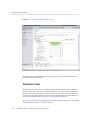
Performance Analyzer Window
This section provides a brief overview of Performance Analyzer's window layout. See
Chapter 4, “Performance Analyzer Tool” and the Help menu for more information about the
functionality and features discussed below.
When you start Performance Analyzer, a Welcome page makes it easy to start profiling an
application in several different ways, view recent experiments, compare experiments, as well as
navigate to documentation.
When you open an experiment, an Overview shows highlights of the data recorded and the set
of metrics available. You can select which metrics you want to examine.
Performance Analyzer is organized around data views that you access from buttons in a
navigation bar on the left side. Each view shows a different perspective of the performance
metrics for your profiled application. The data views are connected so that when you select a
function in one view, the other data views are updated to also focus on that selected function.
In most of the data views, you can use Performance Analyzer's powerful filtering technology to
drill down into performance problems by selecting filters from a context menu or by clicking a
filter button.
See the “Performance Analyzer Views” on page 99 for more information about each view.
You can navigate the Performance Analyzer from the keyboard as well as with a mouse.
20
Oracle Solaris Studio 12.4: Performance Analyzer • January 2015
2
♦ ♦ ♦ C H A P T E R 2 Performance Data
The performance tools record data about specific events while a program is running, and
convert the data into measurements of program performance called metrics. Metrics can be
shown against functions, source lines, and instructions.
This chapter describes the data collected by the performance tools, how it is processed and
displayed, and how it can be used for performance analysis. Because more than one tool
collects performance data, the term Collector is used to refer to any of these tools. Likewise,
because more than one tool analyzes performance data, the term analysis tools is used to refer
to any of these tools.
This chapter covers the following topics.
■
■
“Data the Collector Collects” on page 21
“How Metrics Are Assigned to Program Structure” on page 36
See Chapter 3, “Collecting Performance Data” for information on collecting and storing
performance data.
Data the Collector Collects
The Collector collects various kinds of data using several methods:
■
■
■
■
■
Profiling data is collected by recording profile events at regular intervals. The interval is
either a time interval obtained by using the system clock or a number of hardware events of
a specific type. When the interval expires, a signal is delivered to the system and the data is
recorded at the next opportunity.
Tracing data is collected by interposing a wrapper function on various system functions
and library functions so that calls to the functions can be intercepted and data recorded
about the calls.
Sample data is collected by calling various system routines to obtain global information.
Function and instruction count data is collected for the executable and for any shared
objects that are dynamically opened or statically linked to the executable and instrumented.
The number of times functions and instructions were executed is recorded.
Thread analysis data is collected to support the Thread Analyzer.
Chapter 2 • Performance Data
21
Data the Collector Collects
Both profiling data and tracing data contain information about specific events, and both types
of data are converted into performance metrics. Sample data is not converted into metrics, but
is used to provide markers that can be used to divide the program execution into time segments.
The sample data gives an overview of the program execution during that time segment.
The data packets collected at each profiling event or tracing event include the following
information:
■
■
■
■
■
■
■
A header identifying the data.
A high-resolution timestamp.
A thread ID.
A lightweight process (LWP) ID.
A processor (CPU) ID, when available from the operating system.
A copy of the call stack. For Java programs, two call stacks are recorded: the machine call
stack and the Java call stack.
For OpenMP programs, an identifier for the current parallel region and the OpenMP state
are also collected.
For more information on threads and lightweight processes, see Chapter 6, “Understanding
Performance Analyzer and Its Data”.
In addition to the common data, each event-specific data packet contains information specific to
the data type.
The data types and how you might use them are described in the following subsections:
■
■
■
■
■
■
■
“Clock Profiling Data” on page 22
“Hardware Counter Profiling Data” on page 26
“Synchronization Wait Tracing Data” on page 29
“Heap Tracing (Memory Allocation) Data” on page 30
“I/O Tracing Data” on page 31
“MPI Tracing Data” on page 32
“Sample Data” on page 32
Clock Profiling Data
When you are doing clock profiling, the data collected depends on the information provided by
the operating system.
Clock Profiling Under Oracle Solaris
In clock profiling under Oracle Solaris, the state of each thread is stored at regular time
intervals. This time interval is called the profiling interval. The data collected is converted into
times spent in each state, with a resolution of the profiling interval.
22
Oracle Solaris Studio 12.4: Performance Analyzer • January 2015
Data the Collector Collects
The default profiling interval is approximately 10 milliseconds (10 ms). You can specify a highresolution profiling interval of approximately 1 ms and a low-resolution profiling interval of
approximately 100 ms. If the operating system permits you can also specify a custom interval.
Run the collect -h command with no other arguments to print the range and resolution
allowable on the system.
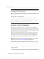
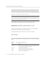
The following table shows the performance metrics that Performance Analyzer and er_print
can display when an experiment contains clock profiling data. Note that the metrics from all
threads are added together.
TABLE 2-1
Timing Metrics from Clock Profiling on Oracle Solaris
Metric
Definition
Total thread time
Sum of time that threads spent in all states.
Total CPU time
Thread time spent running on the CPU in either user, kernel, or trap mode
User CPU time
Thread time spent running on the CPU in user mode.
System CPU time
Thread time spent running on the CPU in kernel mode.
Trap CPU time
Thread time spent running on the CPU in trap mode.
User lock time
Thread time spent waiting for a synchronization lock.
Data page fault time
Thread time spent waiting for a data page.
Text page fault time
Thread time spent waiting for a text page.
Kernel page fault time
Thread time spent waiting for a kernel page.
Stopped time
Thread time spent stopped.
Wait CPU time
Thread time spent waiting for the CPU.
Sleep time
Thread time spent sleeping
Timing metrics tell you where your program spent time in several categories and can be used to
improve the performance of your program.
■
■
■
■
■
■
High user CPU time tells you where the program did most of the work. You can use it
to find the parts of the program where you might gain the most from redesigning the
algorithm.
High system CPU time tells you that your program is spending a lot of time in calls to
system routines.
High wait CPU time tells you that more threads are ready to run than there are CPUs
available, or that other processes are using the CPUs.
High user lock time tells you that threads are unable to obtain the lock that they request.
High text page fault time means that the code ordered by the linker is organized in memory
so that many calls or branches cause a new page to be loaded.
High data page fault time indicates that access to the data is causing new pages to be loaded.
Reorganizing the data structure or the algorithm in your program can fix this problem.
Chapter 2 • Performance Data
23
Data the Collector Collects
Clock Profiling Under Linux
On Linux platforms, the clock data can only be shown as Total CPU time. Linux CPU time is
the sum of user CPU time and system CPU time.
Clock Profiling for OpenMP Programs
If clock profiling is performed on an OpenMP program, additional metrics are provided: Master
Thread Time, OpenMP Work, and OpenMP Wait.
■
■
■
On Oracle Solaris, Master Thread Time is the total time spent in the master thread and
corresponds to wall-clock time. The metric is not available on Linux.
On Oracle Solaris, OpenMP Work accumulates when work is being done either serially
or in parallel. OpenMP Wait accumulates when the OpenMP runtime is waiting for
synchronization, and accumulates whether the wait is using CPU time or sleeping, or when
work is being done in parallel but the thread is not scheduled on a CPU.
On the Linux operating system, OpenMP Work and OpenMP Wait are accumulated only
when the process is active in either user or system mode. Unless you have specified that
OpenMP should do a busy wait, OpenMP Wait on Linux is not useful.
Data for OpenMP programs can be displayed in any of three view modes. In User mode, slave
threads are shown as if they were really cloned from the master thread, and have call stacks
matching those from the master thread. Frames in the call stack coming from the OpenMP
runtime code (libmtsk.so) are suppressed. In Expert user mode, the master and slave threads
are shown differently, and the explicit functions generated by the compiler are visible, and the
frames from the OpenMP runtime code (libmtsk.so) are suppressed. For Machine mode, the
actual native stacks are shown.
Clock Profiling for the Oracle Solaris Kernel
The er_kernel utility can collect clock-based profile data on the Oracle Solaris kernel. You
can profile the kernel by running the er_kernel utility directly from the command line or by
choosing Profile Kernel from the File menu in Performance Analyzer.
The er_kernel utility captures kernel profile data and records the data as an Performance
Analyzer experiment in the same format as an experiment created on user programs by the
collect utility. The experiment can be processed by the er_print utility or Performance
Analyzer. A kernel experiment can show function data, caller-callee data, instruction-level data,
and a timeline, but not source-line data (because most Oracle Solaris modules do not contain
line-number tables).
er_kernel can also record a user-level experiment on any processes running at the time, for
which the user has permissions. Such experiments are similar to experiments that collect
24
Oracle Solaris Studio 12.4: Performance Analyzer • January 2015
Data the Collector Collects
creates but have data only for User CPU Time and System CPU Time, and do not have support
for Java or OpenMP profiling.
See Chapter 9, “Kernel Profiling” for more information.
Clock Profiling for MPI Programs
Clock profiling data can be collected on an MPI experiment that is run with Oracle Message
Passing Toolkit, formerly known as Sun HPC ClusterTools. The Oracle Message Passing
Toolkit must be at least version 8.1.
The Oracle Message Passing Toolkit is available as part of the Oracle Solaris 11 release. If
it is installed on your system, you can find it in /usr/openmpi. If it is not already installed
on your Oracle Solaris 11 system, you can search for the package with the command pkg
search openmpi if a package repository is configured for the system. See Adding and Updating
Software in Oracle Solaris 11 for more information about installing software in Oracle Solaris
11.
When you collect clock profiling data on an MPI experiment, you can view two additional
metrics:
■
■
MPI Work, which accumulates when the process is inside the MPI runtime doing work,
such as processing requests or messages
MPI Wait, which accumulates when the process is inside the MPI runtime but waiting for an
event, buffer, or message
On Oracle Solaris, MPI Work accumulates when work is being done either serially or in
parallel. MPI Wait accumulates when the MPI runtime is waiting for synchronization, and
accumulates whether the wait is using CPU time or sleeping, or when work is being done in
parallel but the thread is not scheduled on a CPU.
On Linux, MPI Work and MPI Wait are accumulated only when the process is active in either
user or system mode. Unless you have specified that MPI should do a busy wait, MPI Wait on
Linux is not useful.
Chapter 2 • Performance Data
25
Data the Collector Collects
Note - If your are using Linux with Oracle Message Passing Toolkit 8.2 or 8.2.1, you might
need a workaround. The workaround is not needed for version 8.1 or 8.2.1c, or for any version
if you are using an Oracle Solaris Studio compiler.
The Oracle Message Passing Toolkit version number is indicated by the installation path such as
/opt/SUNWhpc/HPC8.2.1, or you can type mpirun —V to see output as follows where the version
is shown in italics:
mpirun (Open MPI) 1.3.4r22104-ct8.2.1-b09d-r70
If your application is compiled with a GNU or Intel compiler, and you are using Oracle
Message Passing Toolkit 8.2 or 8.2.1 for MPI, to obtain MPI state data you must use the -WI and
--enable-new-dtags options with the Oracle Message Passing Toolkit link command. These
options cause the executable to define RUNPATH in addition to RPATH, allowing the MPI State
libraries to be enabled with the LD_LIBRARY_PATH environment variable.
Hardware Counter Profiling Data
Hardware counters keep track of events like cache misses, cache stall cycles, floating-point
operations, branch mispredictions, CPU cycles, and instructions executed. In hardware counter
profiling, the Collector records a profile packet when a designated hardware counter of the CPU
on which a thread is running overflows. The counter is reset and continues counting. The profile
packet includes the overflow value and the counter type.
Various processor chip families support from two to eighteen simultaneous hardware counter
registers. The Collector can collect data on one or more registers. For each register you can
select the type of counter to monitor for overflow, and set an overflow value for the counter.
Some hardware counters can use any register, while others are only available on a particular
register. Consequently, not all combinations of hardware counters can be chosen in a single
experiment.
Hardware counter profiling can also be done on the kernel in Performance Analyzer and with
the er_kernel utility. See Chapter 9, “Kernel Profiling” for more information.
Hardware counter profiling data is converted by Performance Analyzer into count metrics. For
counters that count in cycles, the metrics reported are converted to times. For counters that do
not count in cycles, the metrics reported are event counts. On machines with multiple CPUs,
the clock frequency used to convert the metrics is the harmonic mean of the clock frequencies
of the individual CPUs. Because each type of processor has its own set of hardware counters,
and because the number of hardware counters is large, the hardware counter metrics are not
listed here. “Hardware Counter Lists” on page 27 tells you how to find out what hardware
counters are available.
If two specific counters, "cycles" and "insts", are collected, two additional metrics are available,
"CPI" and "IPC", meaning cycles-per-instruction and instructions-per-cycle", respectively. They
26
Oracle Solaris Studio 12.4: Performance Analyzer • January 2015
Data the Collector Collects
are always shown as a ratio, and not as a time, count, or percentage. A high value of CPI or low
value of IPC indicates code that runs inefficiently in the machine; conversely, a low value of
CPI or a high value of IPC indicates code that runs efficiently in the pipeline.
One use of hardware counters is to diagnose problems with the flow of information into and out
of the CPU. High counts of cache misses, for example, indicate that restructuring your program
to improve data or text locality or to increase cache reuse can improve program performance.
Some of the hardware counters correlate with other counters. For example, branch
mispredictions and instruction cache misses are often related because a branch misprediction
causes the wrong instructions to be loaded into the instruction cache. These must be replaced
by the correct instructions. The replacement can cause an instruction cache miss, an instruction
translation lookaside buffer (ITLB) miss, or even a page fault.
For many hardware counters, the overflows are often delivered one or more instructions after
the instruction that caused the overflow event. This situation is referred to as "skid", and it can
make counter overflow profiles difficult to interpret.
On recent SPARC processors, some memory-based counter interrupts are precise, and
are delivered with the PC (program counter) and effective address of the triggering event.
Such counters are indicated by the word precise following the event type. Memoryspace
and dataspace data is captured by default for those counters. See “Dataspace Profiling and
Memoryspace Profiling” on page 183 for more information.
Hardware Counter Lists
Hardware counters are processor-specific, so the choice of counters available depends on the
processor that you are using. The performance tools provide aliases for a number of counters
that are likely to be in common use. You can determine the maximum number of hardware
counters definitions for profiling on the current machine, and see the full list of available
hardware counters, as well as the default counter set, by running collect -h with no other
arguments on the current machine.
If the processor and system support hardware counter profiling, the collect -h command
prints two lists containing information about hardware counters. The first list contains hardware
counters that are aliased to common names. The second list contains raw hardware counters. If
neither the performance counter subsystem nor the collect command have the names for the
counters on a specific system, the lists are empty. In most cases, however, the counters can be
specified numerically.
The following example shows entries in the counter list. The counters that are aliased are
displayed first in the list, followed by a list of the raw hardware counters. Each line of output in
this example is formatted for print.
Aliased HW counters available for profiling:
cycles[/{0|1|2|3}],<interval> (`CPU Cycles', alias for Cycles_user; CPU-cycles)
Chapter 2 • Performance Data
27
Data the Collector Collects
insts[/{0|1|2|3}],<interval> (`Instructions Executed', alias for Instr_all; events)
loads[/{0|1|2|3}],<interval>
(`Load Instructions', alias for Instr_ld; precise load-store events)
stores[/{0|1|2|3}],<interval>
(`Store Instructions', alias for Instr_st; precise load-store events)
dcm[/{0|1|2|3}],<interval>
(`L1 D-cache Misses', alias for DC_miss_nospec; precise load-store events)
l2l3dh[/{0|1|2|3}],<interval>
(`L2 or L3 D-cache Hits', alias for DC_miss_L2_L3_hit_nospec; precise load-store events)
l3m[/{0|1|2|3}],<interval>
(`L3 D-cache Misses', alias for DC_miss_remote_L3_hit_nospec~emask=0x6; precise loadstore events)
l3m_spec[/{0|1|2|3}],<interval>
(`L3 D-cache Misses incl. Speculative', alias for DC_miss_remote_L3_hit~emask=0x6;
events)
.
.
.
Raw HW counters available for profiling:
Sel_pipe_drain_cycles[/{0|1|2|3}],<interval> (CPU-cycles)
Sel_0_wait[/{0|1|2|3}],<interval> (CPU-cycles)
Sel_0_ready[/{0|1|2|3}],<interval> (CPU-cycles)
Sel_1[/{0|1|2|3}],<interval> (CPU-cycles)
Sel_2[/{0|1|2|3}],<interval> (CPU-cycles)
Pick_0[/{0|1|2|3}],<interval> (CPU-cycles)
Pick_1[/{0|1|2|3}],<interval> (CPU-cycles)
Pick_2[/{0|1|2|3}],<interval> (CPU-cycles)
Pick_3[/{0|1|2|3}],<interval> (CPU-cycles)
Pick_any[/{0|1|2|3}],<interval> (CPU-cycles)
Branches[/{0|1|2|3}],<interval> (events)
Instr_FGU_crypto[/{0|1|2|3}],<interval> (events)
Instr_ld[/{0|1|2|3}],<interval> (precise load-store events)
Instr_st[/{0|1|2|3}],<interval> (precise load-store events)
Format of the Aliased Hardware Counter List
In the aliased hardware counter list, the first field (for example, cycles) gives the alias name
that can be used in the -h counter... argument of the collect command. This alias name is also
the identifier to use in the er_print command.
The second field lists the available registers for the counter. For example, [/{0|1|2|3}].
The third field <interval> can be specified as on, hi, or low, or with a numerical value. If
specified as on, hi, or low, and the events are arriving too rapidly, the rate will the throttled
back.
The fourth field, in parentheses, contains type information. It provides a short description (for
example, CPU Cycles), the raw hardware counter name (for example, Cycles_user), and the
type of units being counted (for example, CPU-cycles).
Possible entries in the type information field include the following:
28
Oracle Solaris Studio 12.4: Performance Analyzer • January 2015
Data the Collector Collects
■
precise, the counter interrupt occurs precisely when an instruction causes the event
counter to overflow. The collect -h command for a precise counter collects memoryspace
and dataspace data by default. See “DataObjects View” on page 110, “DataLayout
View” on page 110, and “MemoryObjects Views” on page 109 for details.
■
load, store, or load-store, the counter is memory-related.
■
not-program-related, the counter captures events initiated by some other program, such
as CPU-to-CPU cache snoops. Using the counter for profiling generates a warning and
profiling does not record a call stack.
If the last or only word of the type information is:
■
CPU-cycles, the counter can be used to provide a time-based metric. The metrics reported
for such counters are converted by default to inclusive and exclusive times, but can
optionally be shown as event counts.
■
events, the metric is inclusive and exclusive event counts, and cannot be converted to a
time.
In the aliased hardware counter list in the example, the type information contains the word CPUcycles for the first counter and events for the second counter. For the third counter, the type
information contains two words, load-store events.
Format of the Raw Hardware Counter List
The information included in the raw hardware counter list is a subset of the information in the
aliased hardware counter list. Each line in the raw hardware counter list includes the internal
counter name as used by cputrack(1), the register numbers on which that counter can be used,
the default overflow value, the type information, and the counter units, which can be either CPUcycles or events.
If the counter measures events unrelated to the program running, the first word of
type information is not-program-related. For such a counter, profiling does not
record a call stack, but instead shows the time being spent in an artificial function,
collector_not_program_related . Thread and LWP IDs are recorded, but are meaningless.
The default overflow value for raw counters is 1000003. This value is not ideal for most raw
counters, so you should specify overflow values when specifying raw counters.
Synchronization Wait Tracing Data
In multithreaded programs, the synchronization of tasks performed by different threads can
cause delays in execution of your program. For example, one thread might have to wait for
access to data that has been locked by another thread. These events are called synchronization
Chapter 2 • Performance Data
29
Data the Collector Collects
delay events and are collected by tracing calls to the Solaris or pthread thread functions. The
process of collecting and recording these events is called synchronization wait tracing. The time
spent waiting for the lock is called the wait time.
Events are only recorded if their wait time exceeds a threshold value, which is given in
microseconds. A threshold value of 0 means that all synchronization delay events are traced,
regardless of wait time. The default threshold is determined by running a calibration test, in
which calls are made to the threads library without any synchronization delay. The threshold is
the average time for these calls multiplied by an arbitrary factor (currently 6). This procedure
prevents the recording of events for which the wait times are due only to the call itself
and not to a real delay. As a result, the amount of data is greatly reduced, but the count of
synchronization events can be significantly underestimated.
For Java programs, synchronization tracing covers Java method calls in the profiled program
but does not trace any internal synchronization calls within the JVM.
Synchronization wait tracing data is converted into the metrics in the following table.
TABLE 2-2
Synchronization Wait Tracing Metrics
Metric
Definition
Synchronization delay event count.
The number of calls to a synchronization routine where the wait time
exceeded the prescribed threshold.
Synchronization wait time.
Total of wait times that exceeded the prescribed threshold.
From this information you can determine whether functions or load objects are either frequently
blocked or experience unusually long wait times when they do make a call to a synchronization
routine. High synchronization wait times indicate contention among threads. You can reduce
the contention by redesigning your algorithms, particularly restructuring your locks so that they
cover only the data for each thread that needs to be locked.
Heap Tracing (Memory Allocation) Data
Calls to memory allocation and deallocation functions that are not properly managed can be a
source of inefficient data usage and can result in poor program performance. In heap tracing,
the Collector traces memory allocation and deallocation requests by interposing on the C
standard library memory allocation functions malloc, realloc, valloc, and memalign and the
deallocation function free. Calls to mmap are treated as memory allocations, which enables heap
tracing events for Java memory allocations to be recorded. The Fortran functions allocate and
deallocate call the C standard library functions, so these routines are traced indirectly.
Heap profiling for Java programs is not supported.
Heap tracing data is converted into the following metrics.
30
Oracle Solaris Studio 12.4: Performance Analyzer • January 2015
Data the Collector Collects
TABLE 2-3
Memory Allocation (Heap Tracing) Metrics
Metric
Definition
Allocations
The number of calls to the memory allocation functions
Bytes allocated
The sum of the number of bytes allocated in each call to the memory
allocation functions
Leaks
The number of calls to the memory allocation functions that did not have a
corresponding call to a deallocation function
Bytes leaked
The number of bytes that were allocated but not deallocated
Collecting heap tracing data can help you identify memory leaks in your program or locate
places where there is inefficient allocation of memory.
When you look at the Leaks view with filters applied, the leaks shown are for memory
allocations that were done under the filtering criteria and not deallocated at any time. Leaks are
not restricted to those allocations that are not deallocated under the filtering criteria.
Sometimes, as in the dbx debugging tool, a memory leak is defined as a dynamically allocated
block of memory that has no pointers pointing to it anywhere in the data space of the program.
The definition of leaks used here includes this alternative definition, but also includes memory
for which pointers do exist.
I/O Tracing Data
I/O data collection traces input/output system calls including reads and writes. It measures the
duration of the calls, tracks the files and descriptors, and the amount of data transferred. You
can use the I/O metrics to identify the files, file handles, and call stacks that have high byte
transfer volumes and total thread time.
TABLE 2-4
I/O Tracing Metrics
Metric
Definition
Read Bytes
The sum of the number of bytes read in each call to the read functions.
Write Bytes
The sum of the number of bytes written in each call to the write functions.
Read Count
Number of times read calls were made.
Write Count
Number of times write calls were made.
Other I/O Count
Number of times other IO calls were made
I/O Error Count
Number of errors made during IO calls
Read Time
Number of seconds spent reading data
Write Time
Number of seconds spent writing data
Other I/O Time
Number of seconds spent performing other IO calls
I/O Error Time
Number of seconds spent in IO errors
Chapter 2 • Performance Data
31
Data the Collector Collects
Sample Data
Global data is recorded by the Collector in packets called sample packets. Each packet contains
a header, a timestamp, execution statistics from the kernel such as page fault and I/O data,
context switches, and a variety of page residency (working-set and paging) statistics. The data
recorded in sample packets is global to the program and is not converted into performance
metrics. The process of recording sample packets is called sampling.
Sample packets are recorded in the following circumstances:
■
■
When the program stops for any reason during debugging in dbx, such as at a breakpoint if
the option to do this is set.
At the end of a sampling interval if you have selected periodic sampling. The sampling
interval is specified as an integer in units of seconds. The default value is 1 second.
■
When you use the dbx collector sample record command to manually record a sample.
■
At a call to collector_sample if you have put calls to this routine in your code (see
“Program Control of Data Collection Using libcollector Library” on page 48).
■
When a specified signal is delivered if you have used the -l option with the collect
command (see the collect(1) man page).
When collection is initiated and terminated.
■
■
■
When you pause collection with the dbx collector pause command (just before the
pause) and when you resume collection with the dbx collector resume command (just
after the resume).
Before and after a descendant process is created.
The performance tools use the data recorded in the sample packets to group the data into time
periods, which are called samples. You can filter the event-specific data by selecting a set of
samples so that you see only information for these particular time periods. You can also view
the global data for each sample.
The performance tools make no distinction between the different kinds of sample points.
To make use of sample points for analysis you should choose only one kind of point to be
recorded. In particular, if you want to record sample points that are related to the program
structure or execution sequence, you should turn off periodic sampling and use samples
recorded when dbx stops the process, or when a signal is delivered to the process that is
recording data using the collect command, or when a call is made to the Collector API
functions.
MPI Tracing Data
The Collector can collect data on calls to the Message Passing Interface (MPI) library.
MPI tracing is implemented using the open source VampirTrace 5.5.3 release. It recognizes the
following VampirTrace environment variables:
32
Oracle Solaris Studio 12.4: Performance Analyzer • January 2015
Data the Collector Collects
VT_STACKS
Controls whether call stacks are recorded in the data. The
default setting is 1. Setting VT_STACKS to 0 disables call
stacks.
VT_BUFFER_SIZE
Controls the size of the internal buffer of the MPI API
trace collector. The default value is 64M (64 MBytes).
VT_MAX_FLUSHES
Controls the number of times the buffer is flushed before
terminating MPI tracing. The default value is 0, which
sets the buffer to be flushed to disk whenever it is full.
Setting VT_MAX_FLUSHES to a positive number sets a limit
for the number of times the buffer is flushed.
VT_VERBOSE
Turns on various error and status messages. The default
value is 1, which turns on critical error and status
messages. Set the variable to 2 if problems arise.
For more information on these variables, see the Vampirtrace User Manual on the Technische
Universität Dresden web site.
MPI events that occur after the buffer limits have been reached are not written into the trace file
resulting in an incomplete trace.
To remove the limit and get a complete trace of an application, set the VT_MAX_FLUSHES
environment variable to 0. This setting causes the MPI API trace collector to flush the buffer to
disk whenever the buffer is full.
To change the size of the buffer, set the VT_BUFFER_SIZE environment variable. The optimal
value for this variable depends on the application that is to be traced. Setting a small value
increases the memory available to the application but triggers frequent buffer flushes by the
MPI API trace collector. These buffer flushes can significantly change the behavior of the
application. On the other hand, setting a large value such as 2G minimizes buffer flushes by the
MPI API trace collector but decreases the memory available to the application. If not enough
memory is available to hold the buffer and the application data, parts of the application might be
swapped to disk, leading to a significant change in the behavior of the application.
The following list shows the functions for which data is collected.
MPI_Abort
MPI_Accumulate
MPI_Address
MPI_Allgather
MPI_Allgatherv
MPI_Allreduce
MPI_Alltoall
MPI_Alltoallv
MPI_Alltoallw
MPI_Attr_delete
MPI_Attr_get
MPI_Attr_put
MPI_Barrier
MPI_Bcast
MPI_Bsend
MPI_Bsend-init
MPI_Buffer_attach
MPI_Buffer_detach
MPI_Cancel
MPI_Cart_coords
MPI_Cart_create
MPI_Cart_get
MPI_Cart_map
MPI_Cart_rank
MPI_Cart_shift
MPI_Cart_sub
MPI_Cartdim_get
MPI_Comm_compare
MPI_Comm_create
MPI_Comm_dup
Chapter 2 • Performance Data
33
Data the Collector Collects
34
MPI_Comm_free
MPI_Comm_group
MPI_Comm_rank
MPI_Comm_remote_group
MPI_Comm_remote_size
MPI_Comm_size
MPI_Comm_split
MPI_Comm_test_inter
MPI_Dims_create
MPI_Errhandler_create
MPI_Errhandler_free
MPI_Errhandler_get
MPI_Errhandler_set
MPI_Error_class
MPI_Error_string
MPI_File_close
MPI_File_delete
MPI_File_get_amode
MPI_File_get_atomicity
MPI_File_get_byte_offset
MPI_File_get_group
MPI_File_get_info
MPI_File_get_position
MPI_File_get_position_shared
MPI_File_get_size
MPI_File_get_type_extent
MPI_File_get_view
MPI_File_iread
MPI_File_iread_at
MPI_File_iread_shared
MPI_File_iwrite
MPI_File_iwrite_at
MPI_File_iwrite_shared
MPI_File_open
MPI_File_preallocate
MPI_File_read
MPI_File_read_all
MPI_File_read_all_begin
MPI_File_read_all_end
MPI_File_read_at
MPI_File_read_at_all
MPI_File_read_at_all_begin
MPI_File_read_at_all_end
MPI_File_read_ordered
MPI_File_read_ordered_begin
MPI_File_read_ordered_end
MPI_File_read_shared
MPI_File_seek
MPI_File_seek_shared
MPI_File_set_atomicity
MPI_File_set_info
MPI_File_set_size
MPI_File_set_view
MPI_File_sync
MPI_File_write
MPI_File_write_all
MPI_File_write_all_begin
MPI_File_write_all_end
MPI_File_write_at
MPI_File_write_at_all
MPI_File_write_at_all_begin
MPI_File_write_at_all_end
MPI_File_write_ordered
MPI_File_write_ordered_begin
MPI_File_write_ordered_end
MPI_File_write_shared
MPI_Finalize
MPI_Gather
MPI_Gatherv
MPI_Get
MPI_Get_count
MPI_Get_elements
MPI_Get_processor_name
MPI_Get_version
MPI_Graph_create
MPI_Graph_get
MPI_Graph_map
MPI_Graph_neighbors
MPI_Graph_neighbors_count
MPI_Graphdims_get
MPI_Group_compare
MPI_Group_difference
MPI_Group_excl
MPI_Group_free
MPI_Group_incl
MPI_Group_intersection
MPI_Group_rank
MPI_Group_size
MPI_Group_translate_ranks
MPI_Group_union
MPI_Ibsend
MPI_Init
MPI_Init_thread
MPI_Intercomm_create
MPI_Intercomm_merge
MPI_Irecv
MPI_Irsend
MPI_Isend
MPI_Issend
MPI_Keyval_create
MPI_Keyval_free
MPI_Op_create
MPI_Op_free
MPI_Pack
MPI_Pack_size
MPI_Probe
MPI_Put
MPI_Recv
MPI_Recv_init
MPI_Reduce
MPI_Reduce_scatter
MPI_Request_free
MPI_Rsend
MPI_rsend_init
Oracle Solaris Studio 12.4: Performance Analyzer • January 2015
Data the Collector Collects
MPI_Scan
MPI_Scatter
MPI_Scatterv
MPI_Send
MPI_Send_init
MPI_Sendrecv
MPI_Sendrecv_replace
MPI_Ssend
MPI_Ssend_init
MPI_Start
MPI_Startall
MPI_Test
MPI_Test_cancelled
MPI_Testall
MPI_Testany
MPI_Testsome
MPI_Topo_test
MPI_Type_commit
MPI_Type_contiguous
MPI_Type_extent
MPI_Type_free
MPI_Type_hindexed
MPI_Type_hvector
MPI_Type_indexed
MPI_Type_lb
MPI_Type_size
MPI_Type_struct
MPI_Type_ub
MPI_Type_vector
MPI_Unpack
MPI_Wait
MPI_Waitall
MPI_Waitany
MPI_Waitsome
MPI_Win_complete
MPI_Win_create
MPI_Win_fence
MPI_Win_free
MPI_Win_lock
MPI_Win_post
MPI_Win_start
MPI_Win_test
MPI_Win_unlock
MPI tracing data is converted into the following metrics.
TABLE 2-5
MPI Tracing Metrics
Metric
Definition
MPI Sends
Number of MPI point-to-point sends started
MPI Bytes Sent
Number of bytes in MPI Sends
MPI Receives
Number of MPI point‐to‐point receives completed
MPI Bytes Received
Number of bytes in MPI Receives
MPI Time
Time spent in all calls to MPI functions
Other MPI Events
Number of calls to MPI functions that neither send nor receive point-to-point
messages
MPI Time is the total thread time spent in the MPI function. If MPI state times are also
collected, MPI Work Time plus MPI Wait Time for all MPI functions other than MPI_Init and
MPI_Finalize should approximately equal MPI Work Time. On Linux, MPI Wait and Work are
based on user+system CPU time, while MPI Time is based on real time, so the numbers will not
match.
MPI byte and message counts are currently collected only for point‐to‐point messages. They
are not recorded for collective communication functions. The MPI Bytes Received metric
counts the actual number of bytes received in all messages. MPI Bytes Sent counts the actual
number of bytes sent in all messages. MPI Sends counts the number of messages sent, and MPI
Receives counts the number of messages received.
Chapter 2 • Performance Data
35
How Metrics Are Assigned to Program Structure
Collecting MPI tracing data can help you identify places where you have a performance
problem in an MPI program that could be due to MPI calls. Examples of possible performance
problems are load balancing, synchronization delays, and communications bottlenecks.
How Metrics Are Assigned to Program Structure
Metrics are assigned to program instructions using the call stack that is recorded with the eventspecific data. If the information is available, each instruction is mapped to a line of source code
and the metrics assigned to that instruction are also assigned to the line of source code. See
Chapter 6, “Understanding Performance Analyzer and Its Data” for a more detailed explanation
of how this is done.
In addition to source code and instructions, metrics are assigned to higher‐level objects:
functions and load objects. The call stack contains information on the sequence of function
calls made to arrive at the instruction address recorded when a profile was taken. Performance
Analyzer uses the call stack to compute metrics for each function in the program. These metrics
are called function-level metrics.
Function-Level Metrics: Exclusive, Inclusive, and
Attributed
Performance Analyzer computes three types of function-level metrics: exclusive metrics,
inclusive metrics and attributed metrics.
■
■
■
Exclusive metrics for a function are calculated from events which occur inside the function
itself: they exclude metrics coming from its calls to other functions.
Inclusive metrics are calculated from events which occur inside the function and any
functions it calls: they include metrics coming from its calls to other functions.
Attributed metrics tell you how much of an inclusive metric came from calls from or to
another function: they attribute metrics to another function.
For a function that only appears at the bottom of call stacks (a leaf function), the exclusive and
inclusive metrics are the same.
Exclusive and inclusive metrics are also computed for load objects. Exclusive metrics for a
load object are calculated by summing the function-level metrics over all functions in the load
object. Inclusive metrics for load objects are calculated in the same way as for functions.
Exclusive and inclusive metrics for a function give information about all recorded paths through
the function. Attributed metrics give information about particular paths through a function.
They show how much of a metric came from a particular function call. The two functions
involved in the call are described as a caller and a callee. For each function in the call tree:
36
Oracle Solaris Studio 12.4: Performance Analyzer • January 2015
How Metrics Are Assigned to Program Structure
■
■
The attributed metrics for a function’s callers tell you how much of the function’s inclusive
metric was due to calls from each caller. The attributed metrics for the callers sum to the
function’s inclusive metric.
The attributed metrics for a function’s callees tell you how much of the function’s inclusive
metric came from calls to each callee. Their sum plus the function’s exclusive metric equals
the function’s inclusive metric.
The relationship between the metrics can be expressed by the following equation:
Comparison of attributed and inclusive metrics for the caller or the callee gives further
information:
■
■
The difference between a caller’s attributed metric and its inclusive metric tells you how
much of the metric came from calls to other functions and from work in the caller itself.
The difference between a callee’s attributed metric and its inclusive metric tells you how
much of the callee’s inclusive metric came from calls to it from other functions.
To locate places where you could improve the performance of your program:
■
■
■
Use exclusive metrics to locate functions that have high metric values.
Use inclusive metrics to determine which call sequence in your program was responsible for
high metric values.
Use attributed metrics to trace a particular call sequence to the function or functions that are
responsible for high metric values.
Interpreting Attributed Metrics: An Example
Exclusive, inclusive and attributed metrics are illustrated in Figure 2-1, which contains a
complete call tree. The focus is on the central function, function C.
Pseudo-code of the program is shown after the diagram.
Chapter 2 • Performance Data
37
How Metrics Are Assigned to Program Structure
FIGURE 2-1
38
Call Tree Illustrating Exclusive, Inclusive, and Attributed Metrics
Oracle Solaris Studio 12.4: Performance Analyzer • January 2015
How Metrics Are Assigned to Program Structure
The Main function calls Function A and Function B, and attributes 10 units of its inclusive
metric to Function A and 20 units to function B. These are the callee attributed metrics for
function Main. Their sum (10+20) added to the exclusive metric of function Main equals the
inclusive metric of function main (32).
Function A spends all of its time in the call to function C, so it has 0 units of exclusive metrics.
Function C is called by two functions: function A and function B, and attributes 10 units of its
inclusive metric to function A and 15 units to function B. These are the caller attributed metrics.
Their sum (10+15) equals the inclusive metric of function C (25)
The caller attributed metric is equal to the difference between the inclusive and exclusive
metrics for function A and B, which means they each call only function C. (In fact, the
functions might call other functions but the time is so small that it does not appear in the
experiment.)
Function C calls two functions, function E and function F, and attributes 10 units of its inclusive
metric to function E and 10 units to function F. These are the callee attributed metrics. Their
sum (10+10) added to the exclusive metric of function C (5) equals the inclusive metric of
function C (25).
The callee attributed metric and the callee inclusive metric are the same for function E and for
function F. This means that both function E and function F are only called by function C. The
exclusive metric and the inclusive metric are the same for function E but different for function
F. This is because function F calls another function, Function G, but function E does not.
Pseudo-code for this program is shown below.
main() {
A();
/Do 2 units of work;/
B();
}
A() {
C(10);
}
B() {
C(7.5);
/Do 5 units of work;/
C(7.5);
}
C(arg) {
/Do a total of "arg" units of work, with 20% done in C itself,
40% done by calling E, and 40% done by calling F./
}
Chapter 2 • Performance Data
39
How Metrics Are Assigned to Program Structure
How Recursion Affects Function-Level Metrics
Recursive function calls, whether direct or indirect, complicate the calculation of metrics.
Performance Analyzer displays metrics for a function as a whole, not for each invocation of a
function: the metrics for a series of recursive calls must therefore be compressed into a single
metric. This behavior does not affect exclusive metrics, which are calculated from the function
at the bottom of the call stack (the leaf function), but it does affect inclusive and attributed
metrics.
Inclusive metrics are computed by adding the metric for the event to the inclusive metric of the
functions in the call stack. To ensure that the metric is not counted multiple times in a recursive
call stack, the metric for the event is added only once to the inclusive metric for each unique
function.
Attributed metrics are computed from inclusive metrics. In the simplest case of recursion, a
recursive function has two callers: itself and another function (the initiating function). If all the
work is done in the final call, the inclusive metric for the recursive function is attributed to itself
and not to the initiating function. This attribution occurs because the inclusive metric for all the
higher invocations of the recursive function is regarded as zero to avoid multiple counting of
the metric. The initiating function, however, correctly attributes to the recursive function as a
callee the portion of its inclusive metric due to the recursive call.
40
Oracle Solaris Studio 12.4: Performance Analyzer • January 2015
3
♦ ♦ ♦ C H A P T E R 3 Collecting Performance Data
The first stage of performance analysis is data collection. This chapter describes what is
required for data collection, where the data is stored, how to collect data, and how to manage
the data collection. For more information about the data itself, see Chapter 2, “Performance
Data”.
Data collection is performed from the command line or from the Performance Analyzer tool.
Collecting data at the command line from the kernel requires a separate tool, er_kernel. See
Chapter 9, “Kernel Profiling” for more information.
This chapter covers the following topics.
■
“Compiling and Linking Your Program” on page 41
“Preparing Your Program for Data Collection and Analysis” on page 44
“Limitations on Data Collection” on page 52
“Where the Data Is Stored” on page 56
“Estimating Storage Requirements” on page 59
“Collecting Data” on page 60
■
“Collecting Data Using the collect Command” on page 60
■
“Collecting Data Using the dbx collector Subcommands” on page 80
■
“Collecting Data From a Running Process With dbx on Oracle Solaris
Platforms” on page 86
“Collecting Data From Scripts” on page 88
■
■
■
■
■
■
■
■
“Using collect With ppgsz” on page 89
“Collecting Data From MPI Programs” on page 89
Compiling and Linking Your Program
You can collect and analyze data for a program compiled with almost any compiler option,
but some choices affect what you can collect or what you can see in Performance Analyzer.
The issues to consider when you compile and link your program are described in the following
subsections.
Chapter 3 • Collecting Performance Data
41
Compiling and Linking Your Program
Compiling to Analyze Source Code
To see source code in annotated Source and Disassembly views, and source lines in the Lines
view, you must compile the source files of interest with the -g compiler option (-g0 for C++
to enable front-end inlining) to generate debug symbol information. The format of the debug
symbol information can be either DWARF2 or stabs, as specified by -xdebugformat=(dwarf|
stabs) . The default debug format is dwarf.
Executables and libraries built with DWARF format debugging symbols automatically include
a copy of each constituent object file’s debugging symbols. Executables and libraries built
with stabs format debugging symbols also include a copy of each constituent object file’s
debugging symbols if they are linked with the -xs option, which leaves stabs symbols in the
various object files as well as the executable. The inclusion of this information is particularly
useful if you need to move or remove the object files. With all of the debugging symbols in the
executables and libraries themselves, moving the experiment and the program-related files to a
new location is easier.
Programs can be compiled with the Oracle Solaris Studio compilers or GNU compilers.
However, GNU compilers cannot support some features such as reconstructed call stacks with
OpenMP.
Compiling with -g does not change optimization, except for tail call optimization at the O2 and
O3 optimization levels in Studio compilers.
Source level information for Java code is supported. The location of Java sources, unlike
that for native languages, is not recorded in the experiments. You might need to use path
mapping or set the search path to point to your source. See “How the Tools Find Source
Code” on page 211 for more information.
Compiling for Dataspace and Memoryspace Profiling
Dataspace profiling attributes memory access to data structure elements. To enable dataspace
profiling, you must compile C, C++, and Fortran executables with the Oracle Solaris Studio
compilers and the -xhwcprof option. If you do not compile with this option, the DataObjects
and DataLayout views do not show data for the binaries.
Memoryspace profiling enables you to see which memory addresses are costing the most
performance. No special compiler options are necessary to prepare a program for memoryspace
profiling, but the feature is available only on SPARC platforms running Oracle Solaris 10 1/13,
and on Intel platforms running Oracle Solaris 11.2. See “Dataspace Profiling and Memoryspace
Profiling” on page 183 for more information.
42
Oracle Solaris Studio 12.4: Performance Analyzer • January 2015
Compiling and Linking Your Program
Static Linking
For some types of performance data such as heap tracing and I/O tracing, data collection relies
on a dynamically linked libc. This functionality is lost when you link statically, so you should
not use options such as -dn and -Bstatic with Oracle Solaris Studio compilers.
If you try to collect data for a program that is entirely statically linked, the Collector prints an
error message and does not collect data. The error occurs because the collector library, among
others, is dynamically loaded when you run the Collector.
Do not statically link any of the system libraries or the Collector library, libcollector.so.
Shared Object Handling
Normally the collect command causes data to be collected for all shared objects in the address
space of the target, regardless of whether they are on the initial library list or are explicitly
loaded with dlopen(). However, under some circumstances some shared objects are not
profiled:
■
When the target program is invoked with lazy loading. In such cases, the library is not
loaded at startup time, and is not loaded by explicitly calling dlopen(), so shared object is
not included in the experiment, and all PCs from it are mapped to the <Unknown> function.
The workaround is to set the LD_BIND_NOW environment variable, which forces the library to
be loaded at startup time.
■
When the executable was built with the -B direct option. In this case, the object is
dynamically loaded by a call specifically to the dynamic linker entry point of dlopen(), and
the libcollector interposition is bypassed. The shared object name is not included in the
experiment, and all PCs from it are mapped to the <Unknown>() function. The workaround
is to not use the -B direct option.
Optimization at Compile Time
If you compile your program with optimization turned on at some level, the compiler can
rearrange the order of execution so that it does not strictly follow the sequence of lines in your
program. Performance Analyzer can analyze experiments collected on optimized code, but
the data it presents at the disassembly level is often difficult to relate to the original source
code lines. In addition, the call sequence can appear to be different from what you expect if
the compiler performs tail-call optimizations. See “Tail-Call Optimization” on page 187 for
more information.
Chapter 3 • Collecting Performance Data
43
Preparing Your Program for Data Collection and Analysis
Compiling Java Programs
No special action is required for compiling Java programs with the javac command.
Preparing Your Program for Data Collection and Analysis
You do not need to do anything special to prepare most programs for data collection and
analysis. You should read one or more of the subsections below if your program does any of the
following:
■
■
■
■
■
■
Installs a signal handler. See “Data Collection and Signals” on page 46.
Explicitly dynamically loads a system library. See “Using System
Libraries” on page 45.
Dynamically compiles functions. See “Dynamic Functions and Modules” on page 51.
Creates descendant processes that you want to profile. See “Using System
Libraries” on page 45.
Uses the profiling timer or hardware counter API directly. See “Using System
Libraries” on page 45.
Calls setuid(2) or executes a setuid file. See “Data Collection and
Signals” on page 46 and “Using setuid and setgid” on page 48.
Also, if you want to control data collection from your program during runtime, see “Program
Control of Data Collection Using libcollector Library” on page 48.
Using Dynamically Allocated Memory
Many programs rely on dynamically-allocated memory, using features such as:
■
malloc, valloc, alloca (C/C++)
■
■
new (C++)
Stack local variables (Fortran)
■
MALLOC, MALLOC64 (Fortran)
You must take care to ensure that a program does not rely on the initial contents of dynamically
allocated memory unless the memory allocation method is explicitly documented as setting an
initial value. For example, compare the descriptions of calloc and malloc in the man page for
malloc(3C).
Occasionally, a program that uses dynamically allocated memory might appear to work
correctly when run alone, but might fail when run with performance data collection enabled.
Symptoms might include unexpected floating‐point behavior, segmentation faults, or
application-specific error messages.
44
Oracle Solaris Studio 12.4: Performance Analyzer • January 2015
Preparing Your Program for Data Collection and Analysis
Such behavior might occur if the uninitialized memory is, by chance, set to a benign value
when the application is run alone but is set to a different value when the application is run in
conjunction with the performance data collection tools. In such cases, the performance tools are
not at fault. Any application that relies on the contents of dynamically allocated memory has a
latent bug: an operating system is at liberty to provide any content whatsoever in dynamically
allocated memory unless explicitly documented otherwise. Even if an operating system happens
to always set dynamically allocated memory to a certain value today, such latent bugs might
cause unexpected behavior with a later revision of the operating system, or if the program is
ported to a different operating system in the future.
The following tools may help in finding such latent bugs:
■
Code Analyzer, a Oracle Solaris Studio tool which when used with the compilers and other
tools can show the following:
Static code checking
Code Analyzer can show results of static code checking, which is
performed when you compile your application with the Oracle Solaris
Studio C or C++ compiler and specify the –xanalyze=code option.
Dynamic memory
access checking
Code Analyzer can show results of dynamic memory access
checking, which is performed when you instrument your binary with
discover using the–a option, and then run the instrumented binary to
generate data.
For more information, see “Oracle Solaris Studio 12.4: Code Analyzer User’s Guide ”
■
f95 -xcheck=init_local
For more information, see the “Oracle Solaris Studio 12.4: Fortran User’s Guide ” or the
f95(1) man page.
■
lint utility
For more information, see the “Oracle Solaris Studio 12.4: C User’s Guide ” or the lint(1)
man page.
■
Runtime checking under dbx
For more information, see the “Oracle Solaris Studio 12.4: Debugging a Program With dbx
” manual or the dbx(1) man page.
Using System Libraries
The Collector interposes on functions from various system libraries to collect tracing data and
to ensure the integrity of data collection. The following list describes situations in which the
Collector interposes on calls to library functions.
■
Collecting synchronization wait tracing data. The Collector interposes on functions from the
Oracle Solaris C library, libc.so, on Oracle Solaris.
Chapter 3 • Collecting Performance Data
45
Preparing Your Program for Data Collection and Analysis
■
■
■
■
■
■
Collecting heap tracing data. The Collector interposes on the functions malloc, realloc,
memalign and free. Versions of these functions are found in the C standard library,
libc.so, and also in other libraries such as libmalloc.so and libmtmalloc.so.
Collecting MPI tracing data. The Collector interposes on functions from the specified MPI
library.
Ensuring the integrity of clock data. The Collector interposes on setitimer and prevents
the program from using the profiling timer.
Ensuring the integrity of hardware counter data. The Collector interposes on functions from
the hardware counter library, libcpc.so, and prevents the program from using the counters.
Calls from the program to functions from this library return a value of -1.
Enabling data collection on descendant processes. The Collector interposes on the functions
fork(2), fork1(2), vfork(2), fork(3F), posix_spawn(3p), posix_spawnp(3p), system(3C),
system(3F), sh(3F), popen(3C), and exec(2) and its variants. Calls to vfork are replaced
internally by calls to fork1. These interpositions are done for the collect command.
Guaranteeing the handling of the SIGPROF and SIGEMT signals by the Collector. The
Collector interposes on sigaction to ensure that its signal handler is the primary signal
handler for these signals.
The interposition does not succeed under the following circumstances:
■
Statically linking a program with any of the libraries that contain functions that are
interposed.
■
Attaching dbx to a running application that does not have the collector library preloaded.
Dynamically loading one of these libraries and resolving the symbols by searching only
within the library.
■
The failure of interposition by the Collector can cause loss or invalidation of performance data.
The er_sync.so, er_heap.so, and er_mpviewn.so (where n indicates the MPI version) libraries
are loaded only if synchronization wait tracing data, heap tracing data, or MPI tracing data,
respectively, are requested.
Data Collection and Signals
Signals are used for both clock profiling and hardware counter profiling. SIGPROF is used in
data collection for all experiments. The period for generating the signal depends on the data
being collected. SIGEMT on Solaris or SIGIO on Linux is used for hardware counter profiling.
The overflow interval depends on the user parameter for profiling. Any user code that uses
or manipulates the profiling signals may potentially interfere with data collection. When the
Collector installs its signal handler for a profile signal, it sets a flag that ensures that system
calls are not interrupted to deliver signals. This setting could change the behavior of a target
program that uses the profiling signals for other purposes.
46
Oracle Solaris Studio 12.4: Performance Analyzer • January 2015
Preparing Your Program for Data Collection and Analysis
When the Collector installs its signal handler for a profile signal, it remembers whether or not
the target had installed its own signal handler. The Collector also interposes on some signalhandling routines and does not allow the user to install a signal handler for these signals; it
saves the user's handler, just as it does when the Collector replaces a user handler on starting the
experiment.
Profiling signals are delivered by from the profiling timer or hardware-counter-overflow
handling code in the kernel, or in response to: the kill(2), sigsend(2) tkill(2),
tgkill(2) or _lwp_kill(2) system calls, the raise(3C) and sigqueue(3C) library calls or the
kill command. A signal code is delivered with the signal so that the Collector can distinguish
the origin. If it is delivered for profiling, it is processed by the Collector; If it is not delivered
for profiling, it is delivered to the target signal handler.
When the Collector is running under dbx, the profiling signal delivered occasionally has its
signal code corrupted, and a profile signal may be treated as if it were generated from a system
or library call or a command. In that case, it will be incorrectly delivered to the user's handler. If
the user handler was set to SIG_DFL, it will cause the process to fail core dump.
When the Collector is invoked after attaching to a target process, it will install its signal handler,
but it cannot interpose on the signal-handling routines. If those user code installs a signal
handler after the attach, it will override the Collector's signal handler, and data will be lost.
Note that any signal including either of the profiling signals might cause premature termination
of a system call. The program must be prepared to handle that behavior. When libcollector
installs the signal handlers for data collection it specifies to restart system calls that can be
restarted. However, some system calls such as sleep(3C) return early without reporting an
error.
Sample and Pause-Resume Signals
Signals may be specified by the user as a sample signal (-l) or a pause-resume signal (-y).
SIGUSR1 or SIGUSR2 are recommended for this use, but any signal that is not used by the
target, may be used.
The profiling signals may be used if the process does not otherwise use them, but they should
be used only if no other signal is available. The Collector interposes on some signal-handling
routines and does not allow the user to install a signal handler for these signals; it saves
the user's handler, just as it does when the Collector replaces a user handler on starting the
experiment.
If the Collector is invoked after attaching to a target process, and the user code installs a
signal handler for the sample or pause-resume signal, those signals will not longer operate as
specified.
Chapter 3 • Collecting Performance Data
47
Preparing Your Program for Data Collection and Analysis
Using setuid and setgid
Restrictions enforced by the dynamic loader make it difficult to use setuid(2) and collect
performance data. If your program calls setuid or executes a setuid file, the Collector
probably cannot write an experiment file because it lacks the necessary permissions for the new
user ID.
The collect command operates by inserting a shared library, libcollector.so, into the
target's address space (LD_PRELOAD). Several problems might arise if you invoke the collect
command invoked on executables that call setuid or setgid, or that create descendant
processes that call setuid or setgid. If you are not root when you run an experiment, collection
fails because the shared libraries are not installed in a trusted directory. The workaround is
to run the experiments as root, or use crle(1) to grant permission. Take great care when
circumventing security barriers; you do so at your own risk.
When running the collect command, your umask must be set to allow write permission for
you, for any users or groups that are set by the setuid attributes and setgid attributes of a
program being executed with exec(), and for any user or group to which that program sets
itself. If the mask is not set properly, some files might not be written to the experiment, and
processing of the experiment might not be possible. If the log file can be written, an error is
shown when you attempt to process the experiment.
Other problems can arise if the target itself makes any of the system calls to set UID or GID, or
if it changes its umask and then forks or runs exec() on some other executable, or if crle was
used to configure how the runtime linker searches for shared objects.
If an experiment is started as root on a target that changes its effective GID, the er_archive
process that is automatically run when the experiment terminates fails because it needs a shared
library that is not marked as trusted. In that case, you can run the er_archive utility (or the
er_print utility or the analyzer command) immediately following the termination of the
experiment, on the machine on which the experiment was recorded.
Program Control of Data Collection Using
libcollector Library
If you want to control data collection from your program, the Collector shared library,
libcollector.so contains some API functions that you can use. The functions are written in
C. A Fortran interface is also provided. Both C and Fortran interfaces are defined in header files
that are provided with the library.
The API functions are defined as follows.
void collector_sample(char *name);
void collector_pause(void);
48
Oracle Solaris Studio 12.4: Performance Analyzer • January 2015
Preparing Your Program for Data Collection and Analysis
void collector_resume(void);
void collector_terminate_expt(void);
Similar functionality is provided for Java™ programs by the CollectorAPI class, which is
described in “Java Interface” on page 49.
C and C++ Interface
You can access the C and C++ interface of the Collector API by including collectorAPI.h and
linking with -lcollectorAPI, which contains real functions to check for the existence of the
underlying libcollector.so API functions.
If no experiment is active, the API calls are ignored.
Fortran Interface
The Fortran API libfcollector.h file defines the Fortran interface to the library. The
application must be linked with -lcollectorAPI to use this library. (An alternate name for the
library, -lfcollector, is provided for backward compatibility.) The Fortran API provides the
same features as the C and C++ API, excluding the dynamic function and thread pause and
resume calls.
Insert the following statement to use the API functions for Fortran:
include "libfcollector.h"
Note - Do not link a program in any language with -lcollector. If you do, the Collector might
exhibit unpredictable behavior.
Java Interface
Use the following statement to import the CollectorAPI class and access the Java
API. Note however that your application must be invoked with a classpath pointing to
/installation_directory/lib/collector.jar where installation-directory is the directory in
which the Oracle Solaris Studio software is installed.
import com.sun.forte.st.collector.CollectorAPI;
The Java CollectorAPI methods are defined as follows:
CollectorAPI.sample(String name)
CollectorAPI.pause()
CollectorAPI.resume()
CollectorAPI.terminate()
Chapter 3 • Collecting Performance Data
49
Preparing Your Program for Data Collection and Analysis
The Java API includes the same functions as the C and C++ API, excluding the dynamic
function API.
The C include file libcollector.h contains macros that bypass the calls to the real API
functions if data is not being collected. In this case, the functions are not dynamically loaded.
However, using these macros is risky because the macros do not work well under some
circumstances. Using collectorAPI.h is safer because it does not use macros. Rather, it refers
directly to the functions.
The Fortran API subroutines call the C API functions if performance data is being collected,
otherwise, they return. The overhead for the checking is very small and should not significantly
affect program performance.
To collect performance data you must run your program using the Collector, as described later
in this chapter. Inserting calls to the API functions does not enable data collection.
If you intend to use the API functions in a multithreaded program, ensure that they are called
only by one thread. The API functions perform actions that apply to the process and not to
individual threads. If each thread calls the API functions, the data that is recorded might not
be what you expect. For example, if collector_pause() or collector_terminate_expt()
is called by one thread before the other threads have reached the same point in the program,
collection is paused or terminated for all threads, and data can be lost from the threads that were
executing code before the API call.
C, C++, Fortran, and Java API Functions
This section provides descriptions of the API functions.
■
C and C++: collector_sample(char *name)
Fortran: collector_sample(string name)
Java: CollectorAPI.sample(String name)
Record a sample packet and label the sample with the given name or string. The label is
displayed by Performance Analyzer in the Selection Details window when you select a
sample in the Timeline view. The Fortran argument string is of type character.
Sample points contain data for the process and not for individual threads. In a multithreaded
application, the collector_sample() API function ensures that only one sample is written
if another call is made while it is recording a sample. The number of samples recorded can
be less than the number of threads making the call.
Performance Analyzer does not distinguish between samples recorded by different
mechanisms. If you want to see only the samples recorded by API calls, you should turn off
all other sampling modes when you record performance data.
■
C, C++, Fortran: collector_pause()
Java: CollectorAPI.pause()
50
Oracle Solaris Studio 12.4: Performance Analyzer • January 2015
Preparing Your Program for Data Collection and Analysis
Stop writing event-specific data to the experiment. The experiment remains open, and
global data continues to be written. The call is ignored if no experiment is active or if data
recording is already stopped. This function stops the writing of all event-specific data even
if it is enabled for specific threads by the collector_thread_resume() function.
■
C, C++, Fortran: collector_resume()
Java: CollectorAPI.resume()
Resume writing event-specific data to the experiment after a call to collector_pause() .
The call is ignored if no experiment is active or if data recording is active.
■
C, C++, Fortran: collector_terminate_expt()
Java: CollectorAPI.terminate
Terminate the experiment whose data is being collected. No further data is collected, but the
program continues to run normally. The call is ignored if no experiment is active.
Dynamic Functions and Modules
If your C or C++ program dynamically compiles functions into the data space of the program,
you must supply information to the Collector if you want to see data for the dynamic function
or module in Performance Analyzer. The information is passed by calls to collector API
functions. The definitions of the API functions are as follows.
void collector_func_load(char *name, char *alias,
char *sourcename, void *vaddr, int size, int lntsize,
Lineno *lntable);
void collector_func_unload(void *vaddr);
You do not need to use these API functions for Java methods that are compiled by the Java
HotSpot™ virtual machine, for which a different interface is used. The Java interface provides
the name of the method that was compiled to the Collector. You can see function data and
annotated disassembly listings for Java compiled methods, but not annotated source listings.
This section provides descriptions of the API functions.
collector_func_load() Function
Pass information about dynamically compiled functions to the Collector for recording in the
experiment. The parameter list is described in the following table.
TABLE 3-1
Parameter List for collector_func_load()
Parameter
Definition
name
The name of the dynamically compiled function that is used by the performance tools.
The name does not have to be the actual name of the function. The name need not
Chapter 3 • Collecting Performance Data
51
Limitations on Data Collection
Parameter
Definition
follow any of the normal naming conventions of functions, although it should not
contain embedded blanks or embedded quote characters.
alias
An arbitrary string used to describe the function. It can be NULL. It is not interpreted
in any way, and can contain embedded blanks. It is displayed in the Summary tab of
the Analyzer. It can be used to indicate what the function is, or why the function was
dynamically constructed.
sourcename
The path to the source file from which the function was constructed. It can be NULL.
The source file is used for annotated source listings.
vaddr
The address at which the function was loaded.
size
The size of the function in bytes.
lntsize
A count of the number of entries in the line number table. It should be zero if line
number information is not provided.
lntable
A table containing lntsize entries, each of which is a pair of integers. The first integer
is an offset, and the second entry is a line number. All instructions between an offset in
one entry and the offset given in the next entry are attributed to the line number given
in the first entry. Offsets must be in increasing numeric order, but the order of line
numbers is arbitrary. If lntable is NULL, no source listings of the function are possible,
although disassembly listings are available.
collector_func_unload() Function
Inform the collector that the dynamic function at the address vaddr has been unloaded.
Limitations on Data Collection
This section describes the limitations on data collection that are imposed by the hardware, the
operating system, the way you run your program, or by the Collector itself.
There are no limitations on simultaneous collection of different data types. You can collect any
data type with any other data type, with the exception of count data.
The Collector can support up to 32K user threads. Data from additional threads is discarded,
and a collector error is generated. To support more threads, set the SP_COLLECTOR_NUMTHREADS
environment variable to a larger number.
By default, the Collector collects stacks that are, at most, up to 256 frames deep. If the stack is
deeper, you might see the <Truncated-stack> function in er_print and Performance Analyzer.
See “<Truncated-stack> Function” on page 204 for more information. To support deeper
stacks, set the SP_COLLECTOR_STACKBUFSZ environment variable to a larger number.
52
Oracle Solaris Studio 12.4: Performance Analyzer • January 2015
Limitations on Data Collection
Limitations on Clock Profiling
The minimum value of the profiling interval and the resolution of the clock used for profiling
depend on the particular operating environment. The maximum value is set to 1 second. The
value of the profiling interval is rounded down to the nearest multiple of the clock resolution.
To display the minimum and maximum value and the clock resolution can be found, type the
collect command with no additional arguments.
You cannot do clock profiling on a program that uses the profiling timer. The Collector
intercepts calls to setitimer(3) that set the profiling clock parameters and prevents other
programs from using them.
On Linux platforms, the clock data can only be shown as Total CPU time. Linux CPU time is
the sum of user CPU time and system CPU time.
On Linux systems, clock-profiling of multithreaded applications might report inaccurate
data for threads. The profile signal is not always delivered by the kernel to each thread at the
specified interval; sometimes the signal is delivered to the wrong thread. If available, hardware
counter profiling using the cycle counter will usually give more accurate data for threads.
Runtime Distortion and Dilation With Clock Profiling
Clock profiling records data when a SIGPROF signal is delivered to the target. It causes dilation
to process that signal, and unwind the call stack. The deeper the call stack and the more
frequent the signals, the greater the dilation. To a limited extent, clock profiling shows some
distortion, deriving from greater dilation for those parts of the program executing with the
deepest stacks.
Where possible, a default value is set not to an exact number of milliseconds, but to slightly
more or less than an exact number (for example, 10.007 ms or 0.997 ms) to avoid correlations
with the system clock, which can also distort the data. Set custom values the same way on
Oracle Solaris platforms (not possible on Linux platforms).
Limitations on Collection of Tracing Data
You cannot collect any kind of tracing data from a program that is already running unless the
Collector library, libcollector.so, had been preloaded. See “Collecting Tracing Data From a
Running Program” on page 87 for more information.
Runtime Distortion and Dilation With Tracing
Tracing data dilates the run in proportion to the number of events that are traced. If done with
clock profiling, the clock data is distorted by the dilation induced by tracing events.
Chapter 3 • Collecting Performance Data
53
Limitations on Data Collection
Limitations on Hardware Counter Profiling
Hardware counter profiling has several limitations:
■
■
■
■
You can only collect hardware counter data on processors that have hardware counters and
that support hardware counter profiling. On other systems, hardware counter profiling is
disabled. Oracle Solaris and Oracle Linux with Unbreakable Enterprise Kernel or Red Hatcompatible kernel 6.0 and newer do support hardware counters.
You cannot collect hardware counter data on a system running Oracle Solaris while the
cpustat(1) command is running because cpustat takes control of the counters and does not
let a user process use the counters. If cpustat is started during data collection, the hardware
counter profiling is terminated and an error is recorded in the experiment. The same is true
if root starts an er_kernel experiment using hardware counters.
You cannot use the hardware counters in your own code if you are doing hardware counter
profiling. The Collector interposes on the libcpc library functions and returns with a return
value of -1 if the call did not come from the Collector. Your program should be coded so
as to work correctly if it fails to get access to the hardware counters. If not coded to handle
this, the program will fail under hardware counter profiling, or if the superuser invokes
system-wide tools that also use the counters, or if the counters are not supported on that
system.
If you try to collect hardware counter data on a running program that is using the hardware
counter library by attaching dbx to the process, the experiment may be corrupted.
Note - To view a list of all available counters, run the collect -h command with no additional
arguments.
Runtime Distortion and Dilation With Hardware
Counter Profiling
Hardware counter profiling records data when a SIGEMT signal (on Solaris platforms) or a SIGIO
signal (on Linux platforms) is delivered to the target. It causes dilation to process that signal and
unwind the call stack. Unlike clock profiling, for some hardware counters, different parts of the
program might generate events more rapidly than other parts and show dilation in that part of
the code. Any part of the program that generates such events very rapidly might be significantly
distorted. Similarly, some events might be generated in one thread disproportionately to the
other threads.
54
Oracle Solaris Studio 12.4: Performance Analyzer • January 2015
Limitations on Data Collection
Limitations on Data Collection for Descendant
Processes
You can collect data on descendant processes subject to some limitations.
If you want to collect data for all descendant processes that are followed by the Collector, you
must use the collect command with one of the following options:
■
-F on option enables you to collect data automatically for calls to fork and its variants and
exec and its variants, and all other descendant processes, including those due to calls to
system, popen, posix_spawn(3p), posix_spawnp(3p), and sh
■
-F all is the same as -F on.
■
-F '=regexp' option enables data to be collected on all descendant processes whose name
matches the specified regular expression.
See “Experiment Control Options” on page 71 for more information about the -F option.
Limitations on OpenMP Profiling
Collecting OpenMP data during the execution of the program can be very expensive. You can
suppress that cost by setting the SP_COLLECTOR_NO_OMP environment variable. If you do so, the
program will have substantially less dilation, but you will not see the data from slave threads
propagate up to the caller, and eventually to main(), as it normally will if that variable is not
set.
OpenMP profiling functionality is available only for applications compiled with the Oracle
Solaris Studio compilers because it depends on the Oracle Solaris Studio compiler runtime. For
applications compiled with GNU compilers, only machine-level call stacks are displayed.
Limitations on Java Profiling
You can collect data on Java programs subject to the following limitations:
■
You should use a version of the Java 2 Software Development Kit (JDK) no earlier than
JDK 7, Update 25 (JDK 1.7.0_25). The Collector first looks for the JDK in the path set in
either the JDK_HOME environment variable or the JAVA_PATH environment variable. If neither
of these variables is set, it looks for a JDK in your PATH. If there is no JDK in your PATH, it
looks for the java executable in /usr/java/bin/java.
The Collector verifies that the version of the java executable it finds is an ELF executable.
If it is not, an error message is printed indicating which environment variable or path was
used and the full path name that was tried.
Chapter 3 • Collecting Performance Data
55
Where the Data Is Stored
■
■
You must use the collect command to collect data. You cannot use the dbx collector
subcommands.
Applications that create descendant processes that run JVM software cannot be profiled.
■
Some applications are not pure Java, but are C or C++ applications that invoke dlopen()
to load libjvm.so, and then start the JVM software by calling into it. To profile such
applications, set the SP_COLLECTOR_USE_JAVA_OPTIONS environment variable and add the
-j on option to the collect command line. Do not set the LD_LIBRARY_PATH environment
variable for this scenario.
■
You must use -j on to obtain profiling data if the target is a JVM machine. The -j on
option is not needed if the target is a class or jar file. If you are using a 64-bit JVM machine,
you must specify its path explicitly as the target; do not use the -d64 option for a 32-bit
JVM machine. If the -j on option is specified, but the target is not a JVM machine, an
invalid argument might be passed to the target, and no data would be recorded. The collect
command validates the version of the JVM machine specified for Java profiling.
Runtime Performance Distortion and Dilation for
Applications Written in the Java Programming
Language
Java profiling uses the Java Virtual Machine Tools Interface (JVMTI), which can cause some
distortion and dilation of the run.
For clock profiling and hardware counter profiling, the data collection process makes various
calls into the JVM software and handles profiling events in signal handlers. The overhead of
these routines and the cost of writing the experiments to disk will dilate the runtime of the Java
program. Such dilation is typically less than 10%.
Where the Data Is Stored
The data collected during one execution of your application is called an experiment. The
experiment consists of a set of files that are stored in a directory. The name of the experiment is
the name of the directory.
In addition to recording the experiment data, the Collector creates its own archives of the load
objects used by the program. These archives contain the addresses, sizes, and names of each
object file and each function in the load object, as well as the address of the load object and a
timestamp for its last modification. Archives might also have copies of all shared objects and
some or all of the source files. See “er_archive Utility” on page 239 for more information.
Experiments are stored by default in the current directory. If this directory is on a networked file
system, storing the data takes longer than on a local file system and can distort the performance
56
Oracle Solaris Studio 12.4: Performance Analyzer • January 2015
Where the Data Is Stored
data. You should always try to record experiments on a local file system if possible. You can
specify the storage location when you run the Collector.
Experiments for descendant processes are stored inside the experiment for the founder process.
Experiment Names
The default name for a new experiment is test.1.er . The suffix .er is mandatory: if you
provide a name without this suffix, an error message is displayed and the name is not accepted.
If you choose a name with the format experiment.n.er, where n is a positive integer, the
Collector automatically increments n by one in the names of subsequent experiments. For
example, mytest.1.er is followed by mytest.2.er, mytest.3.er , and so on. The Collector
also increments n if the experiment already exists, and continues to increment n until it finds
an experiment name that is not in use. If the experiment name does not contain n and the
experiment exists, the Collector prints an error message.
Subexperiments follow similar naming rules. See “Subexperiments” on page 177 for more
information.
Experiment Groups
Experiments can be collected into groups. The group is defined in an experiment group file,
which is stored by default in the current directory. The experiment group file is a plain text file
with a special header line and an experiment name on each subsequent line. The default name
for an experiment group file is test.erg. If the name does not end in .erg, an error is displayed
and the name is not accepted. Once you have created an experiment group, any experiments you
run with that group name are added to the group.
To manually create an experiment group file, create a plain text file whose first line is as
follows:
#analyzer experiment group
Then add the names of the experiments on subsequent lines. The file extension must be.erg.
You can also create an experiment group by using the -g argument to the collect command.
Experiments for Descendant Processes
Experiments for descendant processes are named with their lineage as follows. To form the
experiment name for a descendant process, an underscore, a code letter, and a number are added
to the stem of its creator’s experiment name. The code letter is f for a fork, x for an exec, and
Chapter 3 • Collecting Performance Data
57
Where the Data Is Stored
c for combination. The number is the index of the fork or exec (whether successful or not).
For example, if the experiment name for the founder process is test.1.er, the experiment for
the child process created by the third call to fork is test.1.er/_f3.er . If that child process
calls exec successfully, the experiment name for the new descendant process is test.1.er/
_f3_x1.er.
Experiments for MPI Programs
Data for MPI programs are collected by default into test.1.er, and all the data from the MPI
processes are collected into subexperiments, one per rank. The Collector uses the MPI rank
to construct a subexperiment name with the form M_rm.er, where m is the MPI rank. For
example, MPI rank 1 would have its experiment data recorded in the test.1.er/M_r1.er
directory.
Experiments on the Kernel and User Processes
Experiments on the kernel by default are named ktest.1.er rather than test.1.er. When data
is also collected on user processes, the kernel experiment contains subexperiments for each user
process being followed.
The subexperiments are named using the format _process-name_PID_process-id.1.er. For
example an experiment run on a sshd process running under process ID 1264 would be named
ktest.1.er/_sshd_PID_1264.1.er.
Moving Experiments
If you want to move an experiment to another computer to analyze it, you should be aware of
the dependencies of the analysis on the operating environment in which the experiment was
recorded.
The experiment contains all the information necessary to compute metrics at the function level
and to display the timeline. However, if you want to see annotated source code or annotated
disassembly code, you must have access to versions of the load objects or source files that are
identical to the ones used to build the target or the experiment.
See “How the Tools Find Source Code” on page 211 for a description of the process used to
find an experiment's source code.
To ensure that you see the correct annotated source code and annotated disassembly code
for your program, you can copy the source code, the object files, and the executable into the
experiment using the er_archive command before you move or copy the experiment.
58
Oracle Solaris Studio 12.4: Performance Analyzer • January 2015
Estimating Storage Requirements
See the er_archive(1) man page for more information.
Estimating Storage Requirements
This section provides some guidelines for estimating the amount of disk space needed to record
an experiment. The size of the experiment depends directly on the size of the data packets
and the rate at which they are recorded, the number of LWPs used by the program, and the
execution time of the program.
The data packets contain event-specific data and data that depends on the program structure (the
call stack). The amount of data that depends on the data type is approximately 50 to 100 bytes.
The call stack data consists of return addresses for each call, and contains 4 bytes per address,
or 8 bytes per address on 64 bit executables. Data packets are recorded for each thread in the
experiment. Note that for Java programs, there are two call stacks of interest: the Java call stack
and the machine call stack, which therefore result in more data being written to disk.
The rate at which profiling data packets are recorded is controlled by the profiling interval for
clock data, the overflow value for hardware counter data, and, for tracing of functions, the rate
of occurrences of traced functions. The choice of profiling interval parameters affects the data
quality and the distortion of program performance due to the data collection overhead. Smaller
values of these parameters give better statistics but also increase the overhead. The default
values of the profiling interval and the overflow value have been chosen as a compromise
between obtaining good statistics and minimizing the overhead. Smaller values also mean more
data.
For a clock profiling experiment or hardware counter profiling experiment with a profiling
interval of about 100 samples per second, and a packet size ranging from 80 bytes for a small
call stack up to 120 bytes for a large call stack, data is recorded at a rate of 10 kbytes per second
per thread. Applications that have call stacks with a depth of hundreds of calls could easily
record data at ten times these rates.
For MPI tracing experiments, the data volume is 100‐150 bytes per traced MPI call, depending
on the number of messages sent and the depth of the call stack. In addition, clock profiling is
enabled by default when you use the -M option of the collect command, so add the estimated
numbers for a clock profiling experiment. You can reduce data volume for MPI tracing by
disabling clock profiling with the -p off option.
Note - The Collector stores MPI tracing data in its own format (mpview.dat3) and also in
the VampirTrace OTF format (a.otf, a.*.z). You can remove the OTF format files without
affecting Performance Analyzer.
Your estimate of the size of the experiment should also take into account the disk space used by
the archive files (see “Where the Data Is Stored” on page 56). If you are not sure how much
space you need, try running your experiment for a short time. From this test you can obtain the
Chapter 3 • Collecting Performance Data
59
Collecting Data
size of the archive files, which are independent of the data collection time, and scale the size of
the profile files to obtain an estimate of the size for the full-length experiment.
Archives might also have copies of all shared objects and some or all of the source files. See
“er_archive Utility” on page 239 for more information.
As well as allocating disk space, the Collector allocates buffers in memory to store the profile
data before writing it to disk. Currently no way exists to specify the size of these buffers. If the
Collector runs out of memory, try to reduce the amount of data collected.
If your estimate of the space required to store the experiment is larger than the space you
have available, consider collecting data for part of the run rather than the whole run. You can
collect data on part of the run with the collect command with -y or -t options, with the dbx
collector subcommands, or by inserting calls in your program to the collector API. You can
also limit the total amount of profiling and tracing data collected with the collect command
with the -L option, or with the dbx collector subcommands.
See the article Data Selectivity and the Oracle Solaris Studio Performance Analyzer
for information about selective data collection and analysis.
Collecting Data
You can collect performance data on user-mode targets in several ways:
■
■
■
Using the collect command from the command line (see “Collecting Data Using
the collect Command” on page 60 and the collect(1) man page). The collect
command-line tool has smaller data collection overheads than dbx so this method can be
superior to the others.
Using the Profile Application dialog box in Performance Analyzer. (See "Profiling an
Application" in the Performance Analyzer help.)
Using the collector command from the dbx command line. (See “Collecting Data Using
the dbx collector Subcommands” on page 80).
Collecting data automatically on descendant processes can only be done from the Profile
Application dialog box and the collect command.
You can collect performance data on the Oracle Solaris kernel using the er_kernel utility or the
Profile Kernel dialog box. See Chapter 9, “Kernel Profiling” for more information.
Collecting Data Using the collect Command
To run the Collector from the command line using the collect command, type the following.
% collect collect-options program program-arguments
60
Oracle Solaris Studio 12.4: Performance Analyzer • January 2015
Collecting Data Using the collect Command
collect-options are the collect command options, program is the name of the program you
want to collect data on, and program-arguments are the program's arguments. The target
program is typically a binary executable or a script.
If invoked with no arguments, collect displays a usage summary, including the default
configuration of the experiment.
To obtain a list of options and a list of the names of any hardware counters that are available for
profiling, type the collect -h command with no additional arguments.
% collect -h
For a description of the list of hardware counters, see “Hardware Counter Profiling
Data” on page 26. See also “Limitations on Hardware Counter Profiling” on page 54.
Data Collection Options
These options control the types of data that are collected. See “Data the Collector
Collects” on page 21 for a description of the data types.
If you do not specify data collection options, the default is -p on, which enables clock profiling
with the default profiling interval of approximately 10 milliseconds.
If you explicitly disable clock profiling with -p offand do not enable tracing or hardware
counter profiling, the collect command prints a warning message, and collects global
sampling data only.
Clock Profiling with the -p option
With the -p option, you can collect clock profiling data. The allowed values of option are:
■
off – Turn off clock profiling.
■
on – Turn on clock profiling with the default profiling interval of approximately 10
milliseconds.
■
lo[w] – Turn on clock profiling with the low-resolution profiling interval of approximately
100 milliseconds.
■
hi[gh] – Turn on clock profiling with the high-resolution profiling interval of
approximately 1 millisecond. See “Limitations on Clock Profiling” on page 53 for
information on enabling high-resolution profiling.
[+]value – Turn on clock profiling and set the profiling interval to value. The default units
for value are milliseconds. You can specify value as an integer or a floating-point number.
The numeric value can optionally be followed by the suffix m to select millisecond units or
u to select microsecond units. The value should be a multiple of the clock resolution. If the
■
Chapter 3 • Collecting Performance Data
61
Collecting Data Using the collect Command
value is larger but not a multiple, it is rounded down. If it is smaller, a warning message is
printed and it is set to the clock resolution.
Collecting clock profiling data is the default action of the collect command. If you do not
collect count data (-c) or data race and deadlock data (-r) then clock profiling data is collected
even if you do not specify the -p option.
If you specify -h high or -h low to request the default hardware counters to be set for the
processor at high or low-frequency, the default clock profiling is also set to high or low. You
can set a different frequency for clock profiling by explicitly setting it with the -p hi or -p low
or -p n option.
See “Limitations on Clock Profiling” on page 53 for notes about clock-profiling of
multithreaded applications on Linux.
Hardware Counter Profiling with collect -h
Collect hardware counter profiling data. For some hardware, the collect command has defined
a default counter set which you can display using collect -h without any arguments. You can
also specify particular counters instead of using the default counter set. You can use multiple -h
arguments to specify counters.
See “Hardware Counter Lists” on page 27 for information about the format of the counters
displayed with collect -h.
The allowed values of option used with collect -h are:
62
off
Turn off hardware counter profiling. No other options can be specified
with -h off.
on
Turn on hardware counter profiling with the default counter set for the
specific hardware system. If the system does not have a default counter
set, specifying -h on generates an error.
hi | high
Turn on hardware counter profiling for the default counter set for the
system, and profile at a high rate. If the system does not have a default
counter set, specifying -h hi generates an error.
lo | low
Turn on hardware counter profiling for the default counter set for the
system, and profile at a low rate. If the system does not have a default
counter set, specifying -h lo generates an error.
ctr_def...
[,ctr_n_def]
Collect hardware counter profiles using one or more specified counters.
The maximum number of counters supported (ctr_def through ctr_n_def)
is processor-dependent. Run collect -h without any arguments on the
Oracle Solaris Studio 12.4: Performance Analyzer • January 2015
Collecting Data Using the collect Command
current machine to determine the maximum number of hardware counter
definitions for profiling and display the full list of available hardware
counters and the default counter set.
Memory-related counters are those with type load, store, or load-store
as displayed in the counter list when you run the collect -h command
without any other command-line arguments. Some such counters are
also labeled precise. For precise counters on either SPARC or x86,
dataspace and memoryspace data is recorded by default.
Each ctr_def counter definition takes the following form:
ctr[~attr=val]...[~attrN=valN][/reg#],[interval]
The meanings of the counter definition options are as follows:
ctr
Processor-specific counter name shown by running
the collect -h command without any other
command-line arguments. On most systems even
if a counter is not listed it can still be specified by
a numeric value, either in hexadecimal (0x1234)
or decimal. Drivers for older chips do not support
numeric values, but drivers for more recent chips
do. When a counter is specified numerically,
the register number should also be specified.
The numeric values to use are found in the chipspecific manufacturer's manuals. The name of the
manual is given in the collect -h output. Some
counters are only described in proprietary vendor
manuals.
~attr=val
Optional one or more attribute options. On some
processors, attribute options can be associated
with a hardware counter. If the processor supports
attribute options, then running collect -h without
any other command-line arguments will also
provide a list of attribute names to use for ~attr.
The value val can be in decimal or hexadecimal
format. Hexadecimal format numbers are in C
program format where the number is prepended by
a zero and lower-case x (0xhex_number). Multiple
attributes are concatenated to the counter name.
The ~ in front of each attribute name is required.
/reg#
Hardware register to use for the counter. If not
specified, collect attempts to place the counter
into the first available register and as a result,
Chapter 3 • Collecting Performance Data
63
Collecting Data Using the collect Command
might be unable to place subsequent counters due
to register conflicts. If you specify more than one
counter, the counters must use different registers.
You can see a list of allowable register numbers
by running the collect -h command without any
other command-line arguments. The / character is
required if the register is specified.
interval
The interval is the sampling frequency and can be
set to one of the following:
■
on – The default interval, which you can
determine by typing collect -h with no other
arguments. Note that the default value for all
raw counters is the same, and might not be the
most suitable value for a specific counter.
■
hi – The high-resolution value for the chosen
counter, which is approximately ten times
shorter than the default.
■
lo – The low-resolution value for the chosen
counter, which is approximately ten times
longer than the default.
■
value – A specific value, which must be a
positive integer and can be in decimal or
hexadecimal format.
If you omit the interval, the value for -h on is
used. However, if you omit the interval you must
still supply the comma in front of the omitted
interval specification unless you are specifying the
last counter in a -h parameter.
For raw counters, the values for hi, lo, and on, are
guesses, but the appropriate interval is very hard
to guess for any particular program. If you specify
on/hi/lo for any raw counters, and the events
come in faster than 100/1000/10 per second per
thread, respectively, the interval will be throttled
down to a more reasonable maximum on Oracle
Solaris systems.
EXAMPLE 3-1
Valid Examples of -h Usage
-h on
-h lo
64
Oracle Solaris Studio 12.4: Performance Analyzer • January 2015
Collecting Data Using the collect Command
-h hi
Enable the default counters with default, low, or
high rates, respectively
-h cycles,,insts,,dcm
-h cycles -h insts -h dcm
Both have the same meaning: three counters: cycles, insts
and dataspace-profiling of D-cache misses (SPARC only)
-h cycles~system=1
Count cycles in both user and system modes
-h 0xc0/0,10000003
On Nehalem, that is the equivalent to
-h inst_retired.any_p/0,10000003
EXAMPLE 3-2
Invalid Examples of -h Usage
-h cycles -h off
Can't use off with any other -h arguments
-h cycles,insts
Missing comma, and "insts" does not parse as a number for
<interval>
If the -h argument specifies the use of hardware counters but hardware counters are in use
by root at the time the command is given, the collect command will report an error and no
experiment will be run.
If no -h argument is given, no hardware counter profiling data will be collected. An experiment
can specify both hardware counter overflow profiling and clock-based profiling. Specifying
hardware counter overflow profiling will not disable clock-profiling, even is it is enabled by
default.
Synchronization Wait Tracing with -s option
Collect synchronization wait tracing data. The allowed values of option are:
on
Turn on synchronization delay tracing and set the threshold value by calibration at runtime
calibrate
Same as on
off
Turn off synchronization delay tracing
Chapter 3 • Collecting Performance Data
65
Collecting Data Using the collect Command
n
Turn on synchronization delay tracing with a threshold value of n microseconds; if n is
zero, trace all events
all
Turn on synchronization delay tracing and trace all synchronization events
By default, turn off synchronization delay tracing.
For Java programs, synchronization events for Java monitors in user code are recorded, but not
for native synchronization calls within the JVM machine.
On Oracle Solaris, the following functions are traced:
mutex_lock()
rw_rdlock()
rw_wrlock()
cond_wait()
cond_timedwait()
cond_reltimedwait()
thr_join()
sema_wait()
pthread_mutex_lock()
pthread_rwlock_rdlock()
pthread_rwlock_wrlock()
pthread_cond_wait()
pthread_cond_timedwait()
pthread_cond_reltimedwait_np()
pthread_join()
sem_wait()
On Linux, the following functions are traced:
pthread_mutex_lock()
pthread_cond_wait()
pthread_cond_timedwait()
pthread_join()
sem_wait()
Heap Tracing Data with -H option
Collect heap tracing data. The allowed values of option are:
on
66
Turn on tracing of memory allocation requests
Oracle Solaris Studio 12.4: Performance Analyzer • January 2015
Collecting Data Using the collect Command
off
Turn off tracing of memory allocation requests
Heap tracing is turned off by default.
Heap-tracing events are recorded for any native calls and calls to mmap are treated as memory
allocations.
Heap profiling is not supported for Java programs. Specifying it is treated as an error.
Note that heap tracing might produce very large experiments. Such experiments are very slow
to load and browse.
I/O Tracing with -i option
Collect I/O trace data. The allowed values of option are:
on
Turn on tracing of I/O operations
off
Turn off tracing of I/O operations
I/O tracing is not performed by default. I/O tracing might produce very large experiments and
such experiments are very slow to load and browse.
Count Data with -c option
Record count data, for Oracle Solaris systems only.
The allowed values of option are:
on
Turn on count data.
static
Turn on simulated count data, based on the assumption that every
instruction was executed exactly once.
off
Turn off count data.
By default, turn off collection of count data. Count data cannot be collected with any other type
of data.
For count data and simulated count data, the executable and any shared objects that are
instrumented and statically linked are counted. For count data, but not simulated count data,
dynamically loaded shared objects are also instrumented and counted.
Chapter 3 • Collecting Performance Data
67
Collecting Data Using the collect Command
On Oracle Solaris, no special compilation is needed although the count option is incompatible
with compile flags -p, -pg, -qp, -xpg, and --xlinkopt.
On Linux, the executable must be compiled with the -annotate=yes flag in order to collect
count data.
On Oracle Linux 5 instability of the runtime linker audit interface (also called rtld-audit or
LD_AUDIT) might prevent collection of count data.
Specify Count Data Instrumentation Directory with -I directory
Specify a directory for count data instrumentation. This option is available only on Oracle
Solaris systems, and is meaningful only when the -c option is also specified.
Specify Excluded Libraries with -N library-name
Specify a library to be excluded from count data instrumentation, whether the library is linked
into the executable or loaded with dlopen(). This option is available only on Oracle Solaris
systems, and is meaningful only when the -c option is also specified. You can specify multiple
-N options.
Sample Data with -S option
Record sample packets periodically. The allowed values of option are:
off
Turn off periodic sampling.
on
Turn on periodic sampling with the default sampling interval (1 second).
n
Turn on periodic sampling with a sampling interval of n in seconds; n
must be positive.
By default, periodic sampling at 1 second intervals is enabled.
If no data specification arguments are supplied, clock profiling is performed using the default
resolution.
If clock profiling is explicitly disabled, and neither hardware counter overflow profiling nor
any kind of tracing is enabled, collect displays a warning that no function-level data is being
collected, then executes the target and record global data.
68
Oracle Solaris Studio 12.4: Performance Analyzer • January 2015
Collecting Data Using the collect Command
Data Race and Deadlock Detection with -r option
Collect data for data race detection or deadlock detection for the Thread Analyzer.
The allowed values of option are:
race
Collect data for detecting data races.
deadlock
Collect data for detecting deadlocks and potential deadlocks.
all
Collect data for detecting data races, deadlocks, and potential deadlocks. Can also be
specified as race,deadlock.
off
Turn off data collection for data races, deadlocks, and potential deadlocks.
on
Collect data for detecting data races (same as race).
terminate
If an unrecoverable error is detected, terminate the target process.
abort
If an unrecoverable error is detected, terminate the target process with a core dump.
continue
If an unrecoverable error is detected, allow the process to continue.
By default, turn off collection of all Thread Analyzer data. The terminate, abort, and
continue options can be added to any data-collection options, and govern the behavior when
an unrecoverable error occurs, such as a real (not potential) deadlock. The default behavior is
terminate.
Thread Analyzer data cannot be collected with any tracing data, but can be collected in
conjunction with clock- or hardware counter profiling data. Thread Analyzer data significantly
slows down the execution of the target, and profiles might not be meaningful as applied to the
user code.
Thread Analyzer experiments can be examined with either analyzer or with tha. Thread
Analyzer (tha) displays a simplified list of default data views, but is otherwise identical.
Chapter 3 • Collecting Performance Data
69
Collecting Data Using the collect Command
Before you enable data-race detection, you must instrument executables either at compile
time, or by invoking a post- processor. If the target is not instrumented, and none of the shared
objects on its library list is instrumented, a warning is displayed, but the experiment is run.
Other Thread Analyzer data do not require instrumentation.
For more information about the collect -r command and Thread Analyzer, see the “Oracle
Solaris Studio 12.4: Thread Analyzer User’s Guide ” and the tha(1) man page.
MPI Profiling with -M option
Specify collection of an MPI experiment. The target of the collect command must be the
mpirun command, and its options must be separated from the target programs to be run by the
mpirun command by a ‐‐ option. (Always use the ‐‐ option with the mpirun command so that you
can collect an experiment by prepending the collect command and its option to the mpirun
command line.) The experiment is named as usual and is referred to as the founder experiment.
Its directory contains subexperiments for each of the MPI processes, named by rank.
The allowed values of option are:
MPI-version
Turn on collection of an MPI experiment, assuming the MPI version named. The
recognized versions of MPI are printed when you type collect with no arguments, or in
response to an unrecognized version specified with -M.
off
Turn off collection of an MPI experiment.
By default, collection of an MPI experiment is turned off. When collection of an MPI
experiment is turned on, the default setting for the -m option is changed to on.
The supported versions of MPI are printed when you type the collect -h command with no
additional options, or if you specify an unrecognized version with the -M option.
MPI Tracing with -m option
Collect MPI tracing data.
The allowed values of option are:
70
on
Turn on MPI tracing information.
off
Turn off MPI tracing information.
Oracle Solaris Studio 12.4: Performance Analyzer • January 2015
Collecting Data Using the collect Command
MPI tracing is turned off by default unless the -M option is enabled, in which case MPI tracing is
turned on by default. Normally, MPI experiments are collected with the -M option, and no user
control of MPI tracing is needed. If you want to collect an MPI experiment but not collect MPI
tracing data, use the explicit options -M MPI-version -m off.
See “MPI Tracing Data” on page 32 for more information about the MPI functions whose calls
are traced and the metrics that are computed from the tracing data.
Experiment Control Options
These options control aspects of how the experiment data is collected.
Limit the Experiment Size with -L size
Limit the amount of profiling data recorded to size megabytes. The limit applies to the sum of
all profiling data and tracing data, but not to sample points. The limit is only approximate, and
can be exceeded.
When the limit is reached, no more profiling and tracing data is recorded but the experiment
remains open until the target process terminates. If periodic sampling is enabled, sample points
continue to be written.
The allowed values of size are:
unlimited or none
Do not impose a size limit on the experiment.
n
Impose a limit of n megabytes. The value of n must be positive and greater than zero.
By default, there is no limit on the amount of data recorded.
To impose a limit of approximately 2 Gbytes, for example, specify -L 2000.
Follow Processes with the -F option
Control whether descendant processes should have their data recorded. Data is always collected
on the founder process independent of the -F setting. The allowed values of option are:
Chapter 3 • Collecting Performance Data
71
Collecting Data Using the collect Command
on
Record experiments on all descendant processes.
all
Same as on
off
Do not record experiments on any descendant processes.
=regex
Record experiments on those descendant processes whose executable name matches
the regular expression. Only the basename of the executable is used, not the full path. If
the regex that you use contains blanks or characters interpreted by your shell, be sure to
enclose the full regex argument in single quotes.
The -F on option is set by default so that the Collector follows processes created by calls to the
functions fork(2), fork1(2), fork(3F), vfork(2), and exec(2) and its variants. The call to vfork
is replaced internally by a call to fork1.
Descendant processes created by calls to system(3C), system(3F), sh(3F), posix_spawn(3p),
posix_spawnp(3p), and popen(3C), and similar functions, and their associated descendant
processes are also followed.
On Linux, descendants created by clone(2) without the CLONE_VM flag are followed by default.
Descendants created with the CLONE_VM flag are treated as threads rather than processes and are
always followed, independent of the -F setting.
If you specify the -F '= regexp' option, the Collector follows all descendant processes. The
Collector creates a subexperiment when the descendant name or subexperiment name matches
the specified regular expression. See the regexp(5) man page for information about regular
expressions.
Examples using regular expressions:
■
To capture data on the descendant process of the first exec from the first fork from the first
call to system in the founder, use: collect -F '=_x1_f1_x1'
■
To capture data on all the variants of exec, but not fork, use: collect -F '=.*_x[0-9]/*'
To capture data from a call to system ("echo hello") but not system ("goodbye"), use:
collect -F '=echo hello'
■
For more information about how experiments for descendant processes are created and named,
see “Subexperiments” on page 177.
For MPI experiments, descendants are also followed by default.
72
Oracle Solaris Studio 12.4: Performance Analyzer • January 2015
Collecting Data Using the collect Command
Performance Analyzer and the er_print utility automatically read experiments for descendant
processes when the founder experiment is read, and show descendants in the data display.
To select the data of a particular subexperiment for display from the command line, specify the
subexperiment path name explicitly as an argument to the er_print or analyzer commands.
The specified path must include the founder experiment name and the descendant experiment
name inside the founder directory.
For example, to see the data for the third fork of the test.1.er experiment:
er_print test.1.er/_f3.er
analyzer test.1.er/_f3.er
Alternatively, you can prepare an experiment group file with the explicit names of the
descendant experiments in which you are interested. See “Experiment Groups” on page 57
for more information.
Note - If the founder process exits while descendant processes are being followed, collection
of data from descendants that are still running will continue. The founder experiment directory
continues to grow accordingly.
You can also collect data on scripts and follow descendant processes of scripts. See “Collecting
Data From Scripts” on page 88 for more information.
Profile Java with -j option
Enable Java profiling when the target program is a JVM. The allowed values of option are:
on
Record profiling data for the JVM machine, and recognize methods compiled by the Java
HotSpot virtual machine, and also record Java call stacks.
off
Do not record Java profiling data.
path
Record profiling data for the JVM, and use the JVM installed in the specified path.
You must use -j on to obtain profiling data if the target is a JVM machine.
The -j on option is not needed if you want to collect data on a .class file or a .jar file.
Chapter 3 • Collecting Performance Data
73
Collecting Data Using the collect Command
If you are using a 64-bit JVM machine, you must specify its path explicitly as the target; do not
use the -d64 option for a 32-bit JVM machine. If the -j on option is specified, but the target is
not a JVM machine, an invalid argument might be passed to the target, and no data would be
recorded. The collect command validates the version of the JVM machine specified for Java
profiling.
Pass Java Options with -J java-argument
Specify additional arguments to be passed to the JVM used for profiling. If you specify the -J
option, Java profiling (-j on) will be enabled. The java-argument must be enclosed in quotation
marks if it contains more than one argument. It must consist of a set of tokens separated by
blanks or tabs. Each token is passed as a separate argument to the JVM. Most arguments to the
JVM must begin with a dash character (-).
Specify a Signal for Sampling with -l signal
Record a sample packet when the signal named signal is delivered to the process.
You can specify the signal by the full signal name, by the signal name without the initial letters
SIG, or by the signal number. Do not use a signal that is used by the program or that would
terminate execution. Suggested signals are SIGUSR1 and SIGUSR2. SIGPROF can be used even
when clock-profiling is specified. Signals can be delivered to a process by the kill command.
If you use both the -l (a lower case L) and the -y options, you must use different signals for
each option.
If you use this option and your program has its own signal handler, you should make sure that
the signal that you specify with -l is passed on to the Collector’s signal handler and is not
intercepted or ignored.
See the signal(3HEAD) man page for more information about signals.
Set a Time Range with -t duration
Specify a time range for data collection.
The duration can be specified as a single number, with an optional m or s suffix, to indicate
the time in minutes or seconds at which the experiment should be terminated. By default, the
duration is in seconds. The duration can also be specified as two such numbers separated by
74
Oracle Solaris Studio 12.4: Performance Analyzer • January 2015
Collecting Data Using the collect Command
a hyphen, which causes data collection to pause until the first time elapses. At that time, data
collection begins. When the second time is reached, data collection terminates. If the second
number is a zero, data will be collected after the initial pause until the end of the program's run.
Even if the experiment is terminated, the target process is allowed to run to completion.
Stop Profiled Target to Allow dbx attach with -x
Leave the target process stopped on exit from the exec system call in order to allow a debugger
to attach to it. The collect command prints a message with the process ID.
To attach a debugger to the target once it is stopped by collect, you can follow the procedure
below.
1. Obtain the PID of the process from the message printed by the collect -x command
2. Start the debugger
3. Configure the debugger to ignore SIGPROF and, if you chose to collect hardware counter
data, SIGEMT on Solaris or SIGIO on Linux
4. Attach to the process using the dbx attach command.
5. Set the collector parameters for the experiment you wish to collect
6. Issue the collector enable command
7. Issue the cont command to allow the target process to run
As the process runs under the control of the debugger, the Collector records an experiment.
Alternatively, you can attach to the process and collect an experiment using the collect -P
PID command.
Signal Pause and Resume State with -y signal [ ,r]
Control recording of data with the signal named signal. Whenever the signal is delivered to the
process, it switches between the paused state, in which no data is recorded, and the recording
state, in which data is recorded.
By default data collection begins in the paused state. If you specify the optional ,r flag, data
collection begins in the resumed state which means profiling occurs immediately. Sample points
are always recorded, regardless of the state of the -y option.
One use of the pause-resume signal is to start a target without collecting data, allowing it to
reach steady-state, and then enabling the data collection.
Chapter 3 • Collecting Performance Data
75
Collecting Data Using the collect Command
The signal can be specified by the full signal name, by the signal name without the initial letters
SIG, or by the signal number. Do not use a signal that is used by the program or that would
terminate execution. Suggested signals are SIGUSR1 and SIGUSR2. SIGPROF can be used, even
when clock-profiling is specified. Signals can be delivered to a process by the kill command.
If you use both the -l and the -y options, you must use different signals for each option.
When the -y option is used, the Collector is started in the recording state if the optional r
argument is given. Otherwise, it is started in the paused state. If the -y option is not used, the
Collector is started in the recording state.
If you use this option and your program has its own signal handler, make sure that the signal
that you specify with -y is passed on to the Collector’s signal handler, and is not intercepted or
ignored.
See the signal(3HEAD) man page for more information about signals.
Output Options
These options control aspects of the experiment produced by the Collector.
Set Experiment Name with -o experiment-name
Use experiment-name as the name of the experiment to be recorded. The experiment-name
string must end in the string “.er”; if not, the collect utility prints an error message and exits.
If you do not specify the -o option, give the experiment a name of the form stem.n.er, where
stem is a string, and n is a number. If you have specified a group name with the -g option, set
stem to the group name without the .erg suffix. If you have not specified a group name, set
stem to the string test.
If you are invoking the collect command from one of the commands used to run MPI jobs,
for example, mpirun, but without the -M MPI-version option and the -o option, take the value of
n used in the name from the environment variable used to define the MPI rank of that process.
Otherwise, set n to one greater than the highest integer currently in use.
If the name is not specified in the form stem.n.er and the given name is in use, an error
message is displayed and the experiment is not run. If the name is of the form stem.n.er and
the name supplied is in use, the experiment is recorded under a name corresponding to one
greater than the highest value of n that is currently in use. A warning is displayed if the name is
changed.
76
Oracle Solaris Studio 12.4: Performance Analyzer • January 2015
Collecting Data Using the collect Command
Set Directory of Experiment with -d directory-name
Place the experiment in directory directory-name. This option only applies to individual
experiments and not to experiment groups. If the directory does not exist, the collect utility
prints an error message and exits. If a group is specified with the -g option, the group file is also
written to directory-name.
For the lightest-weight data collection,recording data to a local file is best, using the -d option
to specify a directory in which to put the data. However, for MPI experiments on a cluster,
the founder experiment must be available at the same path for all processes to have all data
recorded into the founder experiment.
Experiments written to long-latency file systems are especially problematic and might progress
very slowly, especially if Sample data is collected (-S on option, the default). If you must
record over a long-latency connection, disable Sample data.
Create Experiment in a Group with -g group-name
Make the experiment part of experiment group group-name. If group-name does not end in
.erg, the collect utility prints an error message and exits. If the group exists, the experiment
is added to it. If group-name is not an absolute path, the experiment group is placed in the
directory directory-name if a directory has been specified with -d., Otherwise, it is placed in the
current directory.
Archive Load Objects in Experiment with the -A option
Control whether load objects used by the target process should be archived or copied into the
recorded experiment. The allowed values of option are:
■
on – Copy load objects (the target and any shared objects it uses) into the experiment. Also
copy any .anc files and .o files that have Stabs or DWARF debugging information that is
not in the load object. This is the default.
■
src–In addition to copying load objects as in -A on, copy into the experiment all source
files and .anc files that can be found.
■
used[src]–In addition to copying load objects as in -A on, copy into the experiment all
source files and .anc files that are referenced in the recorded data and can be found.
■
off – Do not copy or archive load objects into the experiment.
If you expect to copy experiments to a different machine, or to read the experiments from a
different machine, specify -A on. The experiment will use more disk space but allows the
experiment to be read on other machines.
Chapter 3 • Collecting Performance Data
77
Collecting Data Using the collect Command
-A on does not copy any source files or object (.o) files into the experiment. You must ensure
that those files are accessible from the machine on which you are examining the experiment.
The files should not be changed or rebuilt after the experiment was recorded.
Archiving of an experiment at collection time, especially for experiments with many descendant
processes, can be very expensive. A better strategy for such an experiment is to collect the data
with -A off, and then run er_archive with the -A flag after the run is terminated.
The default setting for -A is on.
Save the Command Output to a File with -O file
Append all output from collect itself to the named file, but do not redirect the output from the
spawned target, nor from dbx (as invoked with the -P option), nor from the processes involved
in recording count data (as invoked with the -c argument). If file is set to /dev/null, suppress
all output from collect, including any error messages.
Other Options
These collect command options are used for miscellaneous purposes.
Attach to a Process with -P process-id
Write a script for dbx to attach to the process with the given process-id, collect data from it, and
then invoke dbx with that script.
Clock or hardware counter profiling data can be specified, but neither tracing nor count data are
supported. See the collector(1) man page for more information.
When attaching to a process, the directory is created with the umask of the user running
collect -P, but the experiment is written as the user running the process to which dbx
attaches. If the user doing the attach is root, and the umask is not zero, the experiment will fail.
Add a Comment to the Experiment with -C comment
Put the comment into the notes file inside the experiment. You can supply up to ten -C options.
The contents of the notes file are prepended to the experiment header.
78
Oracle Solaris Studio 12.4: Performance Analyzer • January 2015
To Collect Data From a Running Process Using the collect Utility
Try Out a Command with -n
Do not run the target but print the details of the experiment that would be generated if the target
were run. This option is a dry run option.
Display the collect Version with -V
Print the current version of the collect command. No further arguments are examined, and no
further processing is done.
Display Verbose Output with -v
Print the current version of the collect command and detailed information about the
experiment being run.
Collecting Data From a Running Process Using
the collect Utility
On Oracle Solaris platforms only, the -P pid option can be used with the collect utility to
attach to the process with the specified PID, and collect data from the process. The other
options to the collect command are translated into a script for dbx, which is then invoked
to collect the data. Only clock profile data (-p option) and hardware counter profile data (-h
option) can be collected. Tracing data is not supported.
If you use the -h option without explicitly specifying a -p option, clock profiling is turned off.
To collect both hardware counter data and clock data, you must specify both a -h option and a p option.
To Collect Data From a Running Process Using
the collect Utility
1.
Determine the program's process ID (PID).
If you started the program from the command line and put it in the background, its PID will
be printed to standard output by the shell. Otherwise, you can determine the program's PID by
typing the following command.
% ps -ef | grep program-name
Chapter 3 • Collecting Performance Data
79
Collecting Data Using the dbx collector Subcommands
2.
Use the collect command to enable data collection on the process, and set any
optional parameters.
% collect -P pid collect-options
The collector options are described in “Data Collection Options” on page 61. For
information about clock profiling, see “Clock Profiling with the -p option” on page 61. For
information about hardware clock profiling, see “Hardware Counter Profiling with collect -h
” on page 62 .
Collecting Data Using the dbx collector Subcommands
This section shows how to run the Collector from dbx, and then explains each of the
subcommands that you can use with the collector command within dbx.
To Run the Collector From dbx
1.
Load your program into dbx by typing the following command.
% dbx program
2.
Use the collector command to enable data collection, select the data types, and
set any optional parameters.
(dbx) collector subcommand
To see a listing of available collector subcommands, type:
(dbx) help collector
You must use one collector command for each subcommand.
3.
Set up any dbx options and run the program.
If a subcommand is incorrectly given, a warning message is printed and the subcommand is
ignored. The following section provides a complete listing of the collector subcommands.
Data Collection Subcommands
The following subcommands can be used with the collector command within dbx to control
the types of data that are collected by the Collector. They are ignored with a warning if an
experiment is active.
80
Oracle Solaris Studio 12.4: Performance Analyzer • January 2015
To Run the Collector From dbx
profile option
Controls the collection of clock profiling data. The allowed values for option are:
■
on – Enables clock profiling with the default profiling interval of 10 ms.
■
off – Disables clock profiling.
■
timer interval - Sets the profiling interval. The allowed values of interval are:
■
on – Use the default profiling interval of approximately 10 milliseconds.
■
lo[w] – Use the low-resolution profiling interval of approximately 100 milliseconds.
■
hi[gh] – Use the high-resolution profiling interval of approximately 1 millisecond.
See “Limitations on Clock Profiling” on page 53 for information on enabling highresolution profiling.
value - Set the profiling interval to value. The default units for value are milliseconds.
You can specify value as an integer or a floating-point number. The numeric value
can optionally be followed by the suffix m to select millisecond units or u to select
microsecond units. The value should be a multiple of the clock resolution. If the value
is larger than the clock resolution but not a multiple, it is rounded down. If the value is
smaller than the clock resolution it is set to the clock resolution. In both cases, a warning
message is printed.
■
The default setting is approximately 10 milliseconds.
The Collector collects clock profiling data by default, unless the collection of hardwarecounter profiling data is turned on using the hwprofile subcommand.
hwprofile option
Controls the collection of hardware counter profiling data. If you attempt to enable hardware
counter profiling on systems that do not support it, dbx returns a warning message and the
command is ignored. The allowed values for option are:
■
on – Turns on hardware counter profiling. The default action is to collect data for the
cycles counter at the normal overflow value.
■
off – Turns off hardware counter profiling.
■
list – Returns a list of available counters. See “Hardware Counter Lists” on page 27 for
a description of the list. If your system does not support hardware counter profiling, dbx
returns a warning message.
■
counter counter-definition... [, counter-definition ] – A counter definition takes the
following form.
[+]counter-name[~ attribute_1=value_1]...[~attribute_n =value_n][/ register-number]
[,interval ]
Chapter 3 • Collecting Performance Data
81
To Run the Collector From dbx
Selects the hardware counter name and sets its overflow value to interval; optionally selects
additional hardware counter names and sets their overflow values to the specified intervals.
The overflow value can be one of the following:
■
on, or a null string – The default overflow value, which you can determine by typing
collect -h with no additional arguments.
■
hi[gh] – The high-resolution value for the chosen counter, which is approximately ten
times shorter than the default overflow value. The abbreviation h is also supported for
compatibility with previous software releases.
■
lo[w] – The low-resolution value for the chosen counter, which is approximately ten
times longer than the default overflow value.
interval – A specific overflow value, which must be a positive integer and can be in
decimal or hexadecimal format.
■
If you specify more than one counter, each counter must use different registers. If they
do not, a warning message is printed and the command is ignored.
If the hardware counter counts events that relate to memory access, you can prefix the
counter name with a + sign to turn on searching for the true PC of the instruction that
caused the counter overflow. If the search is successful, the PC and the effective address
that was referenced are stored in the event data packet.
The Collector does not collect hardware counter profiling data by default. If hardwarecounter profiling is enabled and a profile command has not been issued, clock
profiling is turned off.
See also “Limitations on Hardware Counter Profiling” on page 54.
synctrace option
Controls the collection of synchronization wait tracing data. The allowed values for option are:
■
on – Enable synchronization wait tracing with the default threshold.
■
off – Disable synchronization wait tracing.
■
threshold value - Sets the threshold for the minimum synchronization delay. The allowed
values for value are:
■
all – Use a zero threshold. This option forces all synchronization events to be recorded.
■
calibrate – Set the threshold value by calibration at runtime. (Equivalent to on.)
■
off – Turn off synchronization wait tracing.
■
on – Use the default threshold, which is to set the value by calibration at runtime.
(Equivalent to calibrate.)
number - Set the threshold to number, given as a positive integer in microseconds. If
value is 0, all events are traced.
■
By default, the Collector does not collect synchronization wait tracing data.
82
Oracle Solaris Studio 12.4: Performance Analyzer • January 2015
To Run the Collector From dbx
heaptrace option
Controls the collection of heap tracing data. The allowed values for option are:
■
on – Enable heap tracing.
■
off – Disable heap tracing.
By default, the Collector does not collect heap tracing data.
tha option
Collect data for data race detection or deadlock detection for the Thread Analyzer. The allowed
values are:
■
off – Turn off thread analyzer data collection.
■
all – Collect all thread analyzer data.
■
race – Collect data-race-detection data.
■
deadlock – Collect deadlock and potential-deadlock data.
For more information about the Thread Analyzer, see the “Oracle Solaris Studio 12.4: Thread
Analyzer User’s Guide ” and the tha.1 man page.
sample option
Controls the sampling mode. The allowed values for option are:
■
periodic – Enable periodic sampling.
■
manual – Disable periodic sampling. Manual sampling remains enabled.
■
period value – Set the sampling interval to value, given in seconds.
By default, periodic sampling is enabled, with a sampling interval value of 1 second.
dbxsample { on | off }
Controls the recording of samples when dbx stops the target process. The meanings of the
keywords are as follows:
■
on – A sample is recorded each time dbx stops the target process.
■
off – Samples are not recorded when dbx stops the target process.
Chapter 3 • Collecting Performance Data
83
To Run the Collector From dbx
By default, samples are recorded when dbx stops the target process.
Experiment Control Subcommands
The following subcommands can be used with the collector command within dbx to control
the collection of experiment data by the Collector. The subcommands are ignored with a
warning if an experiment is active.
disable Subcommand
Disable data collection. If a process is running and collecting data, it terminates the experiment
and disables data collection. If a process is running and data collection is disabled, it is ignored
with a warning. If no process is running, it disables data collection for subsequent runs.
enable Subcommand
Enable data collection. If a process is running but data collection is disabled, it enables data
collection and starts a new experiment. If a process is running and data collection is enabled,
it is ignored with a warning. If no process is running, it enables data collection for subsequent
runs.
You can enable and disable data collection as many times as you like during the execution of
any process. Each time you enable data collection, a new experiment is created.
pause Subcommand
Suspends the collection of data but leaves the experiment open. Sample points are not recorded
while the Collector is paused. A sample is generated prior to a pause, and another sample is
generated immediately following a resume. This subcommand is ignored if data collection is
already paused.
resume Subcommand
Resumes data collection after a pause has been issued. This subcommand is ignored if data is
being collected.
84
Oracle Solaris Studio 12.4: Performance Analyzer • January 2015
To Run the Collector From dbx
sample record name Subcommand
Record a sample packet with the label name. The label is displayed in the Selection Details
window of Performance Analyzer.
Output Subcommands
The following subcommands can be used with the collector command within dbx to define
storage options for the experiment. The subcommands are ignored with a warning if an
experiment is active.
archive mode Subcommand
Set the mode for archiving the experiment. The allowed values for mode are:
■
on – Normal archiving of load objects
■
off – No archiving of load objects
■
copy – Copy load objects into experiment in addition to normal archiving
If you intend to move the experiment to a different machine or read it from another machine,
you should enable the copying of load objects. If an experiment is active, the command is
ignored with a warning. This command does not copy source files or object files into the
experiment.
limit value Subcommand
Limit the amount of profiling data recorded to value megabytes. The limit applies to the sum of
the amounts of clock profiling data, hardware counter profiling data, and synchronization wait
tracing data, but not to sample points. The limit is only approximate, and can be exceeded.
When the limit is reached, no more profiling data is recorded but the experiment remains open
and sample points continue to be recorded.
By default, the amount of data recorded is unlimited.
store option Subcommand
Governs where the experiment is stored. This command is ignored with a warning if an
experiment is active. The allowed values for option are:
Chapter 3 • Collecting Performance Data
85
Collecting Data From a Running Process With dbx on Oracle Solaris Platforms
■
directory directory-name – Sets the directory where the experiment and any experiment
group is stored. This subcommand is ignored with a warning if the directory does not exist.
■
experiment experiment-name – Sets the name of the experiment. If the experiment name
does not end in .er, the subcommand is ignored with a warning. See “Where the Data Is
Stored” on page 56 for more information on experiment names and how the Collector
handles them.
■
group group-name – Sets the name of the experiment group. If the group name does not
end in .erg, the subcommand is ignored with a warning. If the group already exists, the
experiment is added to the group. If the directory name has been set using the store
directory subcommand and the group name is not an absolute path, the group name is
prefixed with the directory name.
Information Subcommands
The following subcommands can be used with the collector command within dbx to get
reports about Collector settings and experiment status.
show Subcommand
Shows the current setting of every Collector control.
status Subcommand
Reports on the status of any open experiment.
Collecting Data From a Running Process With dbx on Oracle
Solaris Platforms
On Oracle Solaris platforms, the Collector allows you to collect data from a running process.
If the process is already under the control of dbx, you can pause the process and enable data
collection using the methods described in previous sections. Starting data collection on a
running process is not supported on Linux platforms.
If the process is not under the control of dbx, the collect –P pid command can be used
to collect data from a running process, as described in “Collecting Data From a Running
Process Using the collect Utility” on page 79. You can also attach dbx to it, collect
performance data, and then detach from the process, leaving it to continue. If you want to
86
Oracle Solaris Studio 12.4: Performance Analyzer • January 2015
To Collect Data From a Running Process That Is Not Under the Control of dbx
collect performance data for selected descendant processes, you must attach dbx to each
process.
To Collect Data From a Running Process That Is
Not Under the Control of dbx
1.
Determine the program’s process ID (PID).
If you started the program from the command line and put it in the background, its PID will
be printed to standard output by the shell. Otherwise you can determine the program’s PID by
typing the following command:
% ps -ef | grep program-name
2.
Attach to the process.
From dbx, type the following command:
(dbx) attach program-name pid
If dbx is not already running, type the following command:
% dbx program-name pid
Attaching to a running process pauses the process.
See the manual “Oracle Solaris Studio 12.4: Debugging a Program With dbx ” for more
information about attaching to a process.
3.
Start data collection.
From dbx, use the collector command to set up the data collection parameters and the cont
command to resume execution of the process.
4.
Detach from the process.
When you have finished collecting data, pause the program and then detach the process from
dbx.
From dbx, type the following command:
(dbx) detach
Collecting Tracing Data From a Running Program
If you want to collect any kind of tracing data, you must preload the Collector library,
libcollector.so , before you run your program. To collect heap tracing data or
Chapter 3 • Collecting Performance Data
87
Collecting Data From Scripts
synchronization wait tracing data, you must also preload er_heap.so and er_sync.so,
respectively. These libraries provide wrappers to the real functions that enable data collection
to take place. In addition, the Collector adds wrapper functions to other system library calls
to guarantee the integrity of performance data. If you do not preload the libraries, these
wrapper functions cannot be inserted. See “Using System Libraries” on page 45 for more
information on how the Collector interposes on system library functions.
To preload libcollector.so, you must set both the name of the library and the path to the
library using environment variables, as shown in the table below. Use the environment variable
LD_PRELOAD to set the name of the library. Use the environment variables LD_LIBRARY_PATH,
LD_LIBRARY_PATH_32, or LD_LIBRARY_PATH_64 to set the path to the library. LD_LIBRARY_PATH
is used if the _32 and _64 variants are not defined. If you have already defined these
environment variables, add new values to them.
TABLE 3-2
Environment Variable Settings for Preloading libcollector.so, er_sync.so, and
er_heap.so
Environment Variable
Value
LD_PRELOAD
libcollector.so
LD_PRELOAD
er_heap.so
LD_PRELOAD
er_sync.so
LD_LIBRARY_PATH
/opt/solarisstudio12.4/lib/analyzer/runtime
LD_LIBRARY_PATH_32
/opt/solarisstudio12.4/lib/analyzer/runtime
LD_LIBRARY_PATH_64
/opt/solarisstudio12.4/lib/analyzer/v9/runtime
LD_LIBRARY_PATH_64
/opt/solarisstudio12.4/lib/analyzer/amd64/runtime
If your Oracle Solaris Studio software is not installed in /opt/solarisstudio12.4, ask your
system administrator for the correct path. You can set the full path in LD_PRELOAD, but doing this
can create complications when using SPARC® V9 64-bit architecture.
Note - Remove the LD_PRELOAD and LD_LIBRARY_PATH settings after the run, so they do not
remain in effect for other programs that are started from the same shell.
Collecting Data From Scripts
You can specify a script as the target for the collect command. When the target is a script,
collect by default collects data on the program that is launched to execute the script, and on all
descendant processes.
To collect data only on a specific process, use the -F option to specify the name of the
executable to follow.
88
Oracle Solaris Studio 12.4: Performance Analyzer • January 2015
Using collect With ppgsz
For example, to profile the script start.sh, but collect data primarily from the executable
myprogram, use the following command.
$ collect -F =myprogram start.sh
Data is collected on the founder process that is launched to execute the start.sh script, and on
all myprogram processes that are spawned from the script, but not collected for other processes.
Using collect With ppgsz
You can use collect with ppgsz(1) by running collect on the ppgsz command and specifying
the -F on or -F all flag. The founder experiment is on the ppgsz executable and uninteresting.
If your path finds the 32-bit version of ppgsz and the experiment is run on a system that
supports 64-bit processes,it will exec its 64-bit version, creating _x1.er. That executable forks,
creating _x1_f1.er.
The child process attempts to exec the named target in the first directory on your path, then
in the second, and so forth, until one of the exec attempts succeeds. If, for example, the
third attempt succeeds, the first two descendant experiments are named _x1_f1_x1.er and
_x1_f1_x2.er, and both are completely empty. The experiment on the target is the one from
the successful exec, the third one in the example, and is named _x1_f1_x3.er, stored under
the founder experiment. It can be processed directly by invoking the Analyzer or the er_print
utility on test.1.er/_x1_f1_x3.er.
If the 64-bit ppgsz is the initial process or if the 32-bit ppgsz is invoked on a 32-bit kernel, the
fork child that execs the real target has its data in _f1.er , and the real target’s experiment is in
_f1_x3.er, assuming the same path properties as in the example above.
Collecting Data From MPI Programs
The Collector can collect performance data from multi-process programs that use the Message
Passing Interface (MPI).
The Collector supports the Oracle Message Passing Toolkit 8 (formerly known as Sun HPC
ClusterTools 8) and its updates. The Collector can recognize other versions of MPI; the list of
valid MPI versions is shown when you run collect -h with no additional arguments.
The Oracle Message Passing Toolkit MPI software is available at http://www.oracle.com/us/
products/tools/message-passing-toolkit-070499.html for installing on Oracle Solaris 10
and Linux systems.
Chapter 3 • Collecting Performance Data
89
Collecting Data From MPI Programs
The Oracle Message Passing Toolkit is made available as part of the Oracle Solaris 11 release.
If it is installed on your system, you can find it in /usr/openmpi. If it is not already installed on
your Oracle Solaris 11 system, you can search for the package with the command pkg search
openmpi if a package repository is configured for the system. See the manual Adding and
Updating Oracle Solaris 11 Software Packages in the Oracle Solaris 11 documentation library
for more information about installing software in Oracle Solaris 11.
For information about MPI and the MPI standard, see the MPI web site http://
www.mcs.anl.gov/mpi/ . For more information about Open MPI, see the web site http://
www.open-mpi.org/ .
To collect data from MPI jobs, you must use the collect command; the dbx collector
subcommands cannot be used to start MPI data collection. Details are provided in “Running the
collect Command for MPI” on page 90.
Running the collect Command for MPI
The collect command can be used to trace and profile MPI applications.
To collect data, use the following syntax:
collect [collect-arguments] mpirun [mpirun-arguments] -- program-name [program-arguments]
For example, the following command runs MPI tracing and profiling on each of the 16 MPI
processes, storing the data in a single MPI experiment:
collect -M OMPT mpirun -np 16 -- a.out 3 5
The -M OMPT option indicates MPI profiling is to be done and Oracle Message Passing Toolkit is
the MPI version.
The initial collect process reformats the mpirun command to specify running the collect
command with appropriate arguments on each of the individual MPI processes.
The ‐‐ argument immediately before the program_name is required for MPI profiling. If you do
not include the ‐‐ argument, the collect command displays an error message and no experiment
is collected.
Note - The technique of using the mpirun command to spawn explicit collect commands on
the MPI processes is no longer supported for collecting MPI trace data. You can still use this
technique for collecting other types of data.
90
Oracle Solaris Studio 12.4: Performance Analyzer • January 2015
Collecting Data From MPI Programs
Storing MPI Experiments
Because multiprocessing environments can be complex, you should be aware of some issues
about storing MPI experiments when you collect performance data from MPI programs. These
issues concern the efficiency of data collection and storage, and the naming of experiments. See
“Where the Data Is Stored” on page 56 for information on naming experiments, including
MPI experiments.
Each MPI process that collects performance data creates its own subexperiment. While an MPI
process creates an experiment, it locks the experiment directory; all other MPI processes must
wait until the lock is released before they can use the directory. Store your experiments on a file
system that is accessible to all MPI processes.
If you do not specify an experiment name, the default experiment name is used. Within the
experiment, the Collector will create one subexperiment for each MPI rank. The Collector uses
the MPI rank to construct a subexperiment name with the form M_rm.er, where m is the MPI
rank.
If you plan to move the experiment to a different location after it is complete, then specify the
-A copy option with the collect command. To copy or move the experiment, do not use the
UNIX cp or mv command. Instead, use the er_cp or er_mv command as described in Chapter 8,
“Manipulating Experiments”.
MPI tracing creates temporary files in /tmp/a.*.z on each node. These files are removed
during the MPI_finalize() function call. Make sure that the file systems have enough space for
the experiments. Before collecting data on a long-running MPI application, do a short-duration
trial run to verify file sizes. Also see “Estimating Storage Requirements” on page 59 for
information on how to estimate the space needed.
MPI profiling is based on the open source VampirTrace 5.5.3 release. It recognizes several
supported VampirTrace environment variables and a new one, VT_STACKS, which controls
whether call stacks are recorded in the data. For further information on the meaning of these
variables, see the VampirTrace 5.5.3 documentation.
The default value of the environment variable VT_BUFFER_SIZE limits the internal buffer of the
MPI API trace collector to 64 Mbytes. After the limit has been reached for a particular MPI
process, the buffer is flushed to disk if the VT_MAX_FLUSHES limit has not been reached. By
default, VT_MAX_FLUSHES is set to 0. This setting causes the MPI API trace collector to flush the
buffer to disk whenever the buffer is full. If you set VT_MAX_FLUSHES to a positive number, you
limit the number of flushes allowed. If the buffer fills up and cannot be flushed, events are no
longer written into the trace file for that process. The result can be an incomplete experiment,
and, in some cases, the experiment might not be readable.
To change the size of the buffer, use the environment variable VT_BUFFER_SIZE. The optimal
value for this variable depends on the application that is to be traced. Setting a small value will
increase the memory available to the application but will trigger frequent buffer flushes by
Chapter 3 • Collecting Performance Data
91
Collecting Data From MPI Programs
the MPI API trace collector. These buffer flushes can significantly change the behavior of the
application. On the other hand, setting a large value like 2 Gbytes will minimize buffer flushes
by the MPI API trace collector but decrease the memory available to the application. If not
enough memory is available to hold the buffer and the application data, parts of the application
might be swapped to disk, leading also to a significant change in the behavior of the application.
Another important variable is VT_VERBOSE, which turns on various error and status messages.
Set this variable to 2 or higher if problems arise.
Normally, MPI trace output data is post-processed when the mpirun target exits. A processed
data file is written to the experiment and information about the post-processing time is written
into the experiment header. MPI post-processing is not done if MPI tracing is explicitly disabled
with -m off. In the event of a failure in post-processing, an error is reported, and no MPI Tabs
or MPI tracing metrics are available.
If the mpirun target does not actually invoke MPI, an experiment is still recorded but no MPI
trace data is produced. The experiment reports an MPI post-processing error, and no MPI Tabs
or MPI tracing metrics will be available.
If the environment variable VT_UNIFY is set to 0, the post-processing routines are not run by
collect. They are run the first time er_print or analyzer are invoked on the experiment.
Note - If you copy or move experiments between computers or nodes, you cannot view the
annotated source code or source lines in the annotated disassembly code unless you have
access to the source files or a copy with the same timestamp. You can put a symbolic link
to the original source file in the current directory in order to see the annotated source. You
can also use settings in the Settings dialog box. Use the Search Path tab (see “Search Path
Settings” on page 131) to manage a list of directories to be used for searching for source
files. Use the Pathmaps tab (see “Pathmaps Settings” on page 132) to map the leading part of
a file path from one location to another.
92
Oracle Solaris Studio 12.4: Performance Analyzer • January 2015
4
♦ ♦ ♦ C H A P T E R 4 Performance Analyzer Tool
This chapter describes the Performance Analyzer graphical data analysis tool and covers the
following topics:
■
■
■
■
■
■
■
■
■
■
■
“About Performance Analyzer” on page 93
“Starting Performance Analyzer” on page 94
“Performance Analyzer User Interface” on page 97
“Performance Analyzer Views” on page 99
“Setting Library and Class Visibility ” on page 118
“Filtering Data” on page 119
“Profiling Applications From Performance Analyzer” on page 121
“Profiling a Running Process” on page 122
“Comparing Experiments” on page 123
“Using Performance Analyzer Remotely” on page 124
“Configuration Settings” on page 126
About Performance Analyzer
Performance Analyzer is a graphical data-analysis tool that analyzes performance data collected
by the Collector. The Collector starts when you profile an application from Performance
Analyzer, use the collect command, or use the collector commands in dbx. The Collector
gathers performance information to create an experiment during the execution of a process, as
described in Chapter 3, “Collecting Performance Data”.
Performance Analyzer reads in such experiments, analyzes the data, and displays the data in
tabular and graphical displays.
Chapter 4 • Performance Analyzer Tool
93
Starting Performance Analyzer
Note - You can download demonstration code for Performance Analyzer in the sample
applications zip file from the Oracle Solaris Studio 12.4 Sample Applications page at http://
www.oracle.com/technetwork/server-storage/solarisstudio/downloads/solarisstudio-12-4-samples-2333090.html .
After accepting the license and downloading, you can extract the zip file in a directory of
your choice. The sample applications are located in the PerformanceAnalyzer subdirectory
of the SolarisStudioSampleApplications directory. See the “Oracle Solaris Studio 12.4:
Performance Analyzer Tutorials ” for information about how to use the sample code with
Performance Analyzer.
Starting Performance Analyzer
To start Performance Analyzer, type the following command in a terminal window:
% analyzer [control-options] [experiment | experiment-list]
You can specify an experiment name or a list. The experiment-list command argument is a
space-separated list of experiment names, experiment group names, or both. If you do not
provide an experiment list, Performance Analyzer starts and opens the Welcome page.
You can specify multiple experiments or experiment groups on the command line. If you
specify an experiment that has descendant experiments inside it, all descendant experiments are
automatically loaded and the data is aggregated. To load individual descendant experiments,
you must specify each experiment explicitly or create an experiment group. You can also put an
en_desc directive in an .er.rc file (see “en_desc { on | off | =regexp}” on page 168).
In reading experiments with descendants, any sub-experiments that contain little or no
performance data are ignored by Performance Analyzer and er_print.
To create an experiment group, you can use the -g argument to the collect utility. To manually
create an experiment group, create a plain text file whose first line is as follows:
#analyzer experiment group
Then add the names of the experiments on subsequent lines. The file extension must be erg.
When Performance Analyzer displays multiple experiments, data from all the experiments is
aggregated by default. The data is combined and viewed as if the data is from one experiment.
However, you can also choose to compare the experiments instead of aggregating the data if
you specify the -c option. See “Comparing Experiments” on page 123.
You can preview an experiment or experiment group by clicking its name in the Open
Experiment dialog box.
94
Oracle Solaris Studio 12.4: Performance Analyzer • January 2015
Starting Performance Analyzer
You can also start Performance Analyzer from the command line to record an experiment as
follows:
% analyzer [Java-options] [control-options] target [target-arguments]
Performance Analyzer starts up with the Profile Application window showing the named target
and its arguments and settings for profiling an application and collecting an experiment. See
“Profiling Applications From Performance Analyzer” on page 121 for details.
You can also open a “live” experiment – an experiment that is still being collected. When you
open a live experiment, you see only the data that had already been collected when you opened
the experiment. The experiment is not automatically updated as new data comes in. To update,
you can open the experiment again.
analyzer Command Options
These analyzer command options control the behavior of Performance Analyzer and are
divided into the following groups:
■
■
■
■
Experiment options
Java options
Control options
Information options
Experiment Options
These options specify how to handle experiments that you specify on the command line.
-c base-group compare-group
Start Performance Analyzer and compare the specified experiments.
The base-group is either a single experiment or a groupname.erg file which specifies multiple
experiments. The compare-group is one or more experiments that you want to compare to the
base group.
To specify multiple experiments in the compare group, separate the experiment names with
spaces. You can also specify a groupname.erg file which specifies multiple experiments in the
compare group.
EXAMPLE 4-1
Sample Commands for Opening Experiments in Comparison Mode
Open the experiment test.1.er and compare it to test.4.er:
Chapter 4 • Performance Analyzer Tool
95
Starting Performance Analyzer
% analyzer -c test.1.er test.4.er
Open the experiment group demotest.erg and compare it to test.4.er:
% analyzer -c demotest.erg test.4.er
Java Options for analyzer Command
These options specify settings for the JVM that runs Performance Analyzer.
-j | --jdkhome jvm-path
Specify the path to the Java software for running Performance Analyzer. When the -j option is
not specified, the default path is taken first by examining environment variables for a path to
the JVM, in the order JDK_HOME and then JAVA_PATH. If neither environment variable is set, the
JVM found on your PATH is used. Use the -j option to override all the default paths. See
-Jjvm-option
Specify the JVM options. You can specify multiple options. For example:
■
To run the 64–bit Performance Analyzer, type:
analyzer -J-d64
■
To run Performance Analyzer with a maximum of JVM memory of 2 Gbytes, type:
analyzer -J-Xmx2G
■
To run the 64–bit Performance Analyzer with a maximum JVM memory of 8 Gbytes, type:
analyzer -J-d64 -J-Xmx8G
Control Options for analyzer Command
These analyzer command options control the location of the user directory where your
settings are stored, set the font size of the user interface. and display the version and runtime
information before starting Performance Analyzer.
-f | --fontsize size
Specify the font size to be used in the Performance Analyzer user interface..
96
Oracle Solaris Studio 12.4: Performance Analyzer • January 2015
Performance Analyzer User Interface
To start Performance Analyzer and display the menus in 14-point font, type the following:
analyzer -f 14
-v | --verbose
Display version information and Java runtime arguments and then start Performance Analyzer.
Information Options for analyzer Command
These options print information about analyzer to standard output. The individual options
below are stand-alone options. They cannot be combined with other analyzer options nor
combined with target or experiment-list arguments.
-V | --version
Display version information only and do not start Performance Analyzer.
-? | -h | --help
Print usage information and exit.
Performance Analyzer User Interface
The Performance Analyzer window has a menu bar, a toolbar, and a navigation panel. You use
each of these to interact with Performance Analyzer and your data.
Menu Bar
The menu bar contains the following command menus.
■
File provides several options you can use to profile applications, open experiments, and
compare or aggregate data from multiple experiments. Other options include the ability to
export the content of a data view to several different formats and connect to a remote host
use the Performance Analyzer on files and applications located there.
Chapter 4 • Performance Analyzer Tool
97
Performance Analyzer User Interface
■
■
■
Views enables you to select the data views that you want Performance Analyzer to
display in the navigation bar. You can also click the Views + button or More Views in the
navigation bar to add more data views.
Tools provides options for filtering data, hiding library functions in the data views, and
other settings.
Help provides links to integrated documentation for Performance Analyzer including links
to new features, quick reference, keyboard shortcuts, and troubleshooting information. You
can also press the F1 key on your keyboard to display information about the current view in
Performance Analyzer.
Tool Bar
The toolbar provides buttons you can use as shortcuts for commands, a view mode selector that
you can use to change the way data is displayed for Java and OpenMP experiments, and a Find
tool to help you locate text in data views.
FIGURE 4-1
Toolbar of Performance Analyzer
Navigation Panel
The vertical navigation panel on the left enables you to select various pages known as data
views or simply views in Performance Analyzer. Most views show a perspective of the
performance metrics for your profiled application. The views are related so that selections you
make and filters you apply in one view are applied to other views.
Some buttons on the navigation panel open pages such as the Welcome page which makes the
tool easier to use and find information, and the Overview page which provides information
about the data in the open experiments.
You can add more views to the navigation panel by clicking the + button at the top of the
navigation panel or the More Views button on the bottom of the navigation panel. You can also
use the Views menu to select another view to add.
You can click the items in most data views to see more detailed information about the items
in the Selection Details window, which is described in the next section “Selection Details
Window” on page 99.
The data views are described in “Performance Analyzer Views” on page 99.
98
Oracle Solaris Studio 12.4: Performance Analyzer • January 2015
Performance Analyzer Views
Selection Details Window
The Selection Details window on the right side shows all the recorded metrics for the selected
item both as values and percentages, and information on the selected function or load object.
The Selection Details window is updated whenever a new item is selected in any data view.
When you select a sample in the Samples bar of the Timeline view, the Selection Details
window shows the sample number, the start and end time of the sample, and the microstates
with the amount of time spent in each microstate and the color coding.
When you select an event in a data bar of the Timeline view, the Selection Details window
shows the event details and the call stack.
Called-By/Calls Panel
The Called-by/Calls panel at the bottom of some data views enables you to navigate call paths.
Select a function in the view and then use the Called-by/Calls panel to navigate to functions it
was called by, or to function calls it makes. When you click a function in Called-by/Calls, the
function is selected in the data view.
Performance Analyzer Views
The following factors determine whether a data view is displayed in the navigation bar when
you open an experiment:
■
■
The type of data in the experiment determines what data views should be displayed. For
example, if an experiment contains OpenMP data, the views for OpenMP are automatically
opened to display the data.
Configuration files which are read when you start Performance Analyzer specify the default
data views to display.
You can use the Views menu or button to open the Settings dialog box (see “Views
Settings” on page 126) to select the views that you want to display in the current
Performance Analyzer session.
Most views have a context menu that opens when you by right-click on an item in the view. You
can use the context menu to add filters or to perform other activities related to that data view.
When you apply filters in one view, the data is filtered in all the views that can be filtered.
The navigation bar shows the following:
■
■
■
“Welcome Page” on page 100
“Overview Screen” on page 101
“Functions View” on page 102
Chapter 4 • Performance Analyzer Tool
99
Performance Analyzer Views
■
■
■
■
■
■
■
■
■
■
■
■
■
■
■
■
■
■
■
■
■
■
■
■
■
■
■
■
■
■
■
■
“Timeline View” on page 103
“Source View” on page 105
“Call Tree View” on page 106
“Callers-Callees View” on page 106
“Index Objects Views” on page 108
“Threads View” on page 108
“Samples View” on page 108
“CPUs View” on page 108
“Seconds View” on page 109
“Processes View” on page 109
“Experiment IDs View” on page 109
“MemoryObjects Views” on page 109
“DataObjects View” on page 110
“DataLayout View” on page 110
“I/O View” on page 111
“Heap View” on page 111
“Data Size View” on page 112
“Duration View” on page 112
“OpenMP Parallel Region View” on page 112
“OpenMP Task View” on page 113
“Lines View” on page 113
“PCs View” on page 114
“Disassembly View” on page 114
“Source/Disassembly View” on page 115
“Races View” on page 115
“Deadlocks View” on page 115
“Dual-Source View” on page 115
“Inst-Freq View” on page 116
“Statistics View” on page 116
“Experiments View” on page 116
“MPI Timeline View” on page 116
“MPI Chart View” on page 117
Welcome Page
When you start Performance Analyzer without specifying on the command line which
experiment to open, the first page you see if the Welcome page. The Welcome page makes it
easy to start profiling an application, view recent experiments, compare experiments, and view
100
Oracle Solaris Studio 12.4: Performance Analyzer • January 2015
Performance Analyzer Views
documentation. After you open an experiment, you can still select the Welcome page from the
navigation panel at any time during a Performance Analyzer session.
The following figure shows the Welcome page.
FIGURE 4-2
Performance Analyzer Welcome Page
Overview Screen
When you open an experiment Performance Analyzer displays the Overview, which shows
performance metrics for the loaded experiments and can give you a quick idea of where the
metrics are high. Use the Overview to select the metrics you want to explore in other views.
Press F1 while viewing the Overview for detailed information about the Overview.
The following figure shows the Performance Analyzer window with the Overview displayed.
Chapter 4 • Performance Analyzer Tool
101
Performance Analyzer Views
FIGURE 4-3
Performance Analyzer's Overview Screen
As you select metrics, the Metrics Preview panel at the bottom of the window show how the
metrics will look in the data views.
Functions View
The Functions view shows a list of the target program's functions and their metrics, which are
derived from the data collected in the experiment. Metrics can be either exclusive or inclusive.
Exclusive metrics represent usage only by the function itself. Inclusive metrics represent usage
by the function and all the functions it called. For more detailed information about metrics, see
“Function-Level Metrics: Exclusive, Inclusive, and Attributed” on page 36.
The list of available metrics for each kind of data collected is given in the collect(1) man page
and the help, and in Chapter 2, “Performance Data”.
102
Oracle Solaris Studio 12.4: Performance Analyzer • January 2015
Performance Analyzer Views
Time metrics are shown as seconds, presented to millisecond precision. Percentages are shown
to a precision of 0.01%. If a metric value is precisely zero, its time and percentage is shown
as “0.” If the value is not exactly zero but is smaller than the precision, its value is shown as
“0.000” and its percentage as “0.00”. Because of rounding, percentages may not sum to exactly
100%. Count metrics are shown as an integer count.
The metrics initially shown are based on the data collected. If more than one type of data has
been collected, the default metrics for each type are shown. You can select which metrics to
display in the Overview page. See “Overview Screen” on page 101 for more information.
To search for a function, use the Find tool in the toolbar.
To view the source code for a function, double-click on it to open the Source view at the correct
line in the source code.
To select a single function, click that function and see more information about it in the Selection
Details window on the right side.
To select several functions that are displayed contiguously in the view, select the first function
of the group, then Shift-click on the last function of the group.
To select several functions that are not displayed contiguously in the view, select the first
function of the group, then select the additional functions by Control-clicking on each function.
You can also right-click in the Functions view to open a context menu and select a predefined
filter for the selected functions. See the Performance Analyzer help for details about filtering.
Timeline View
The Timeline view shows a chart of the events and the sample points recorded as a function
of time. Data is displayed in horizontal bars. By default, for each experiment there is one bar
for CPU Utilization Samples at the top and a set of profiling data bars for each thread. The
data shown for each thread is determined by the data you collected when you profiled your
application.
You might see the following data bars:
CPU Utilization Samples
When an experiment includes sample data, the top bar displayed is CPU Utilization
Samples. Data in a sample point represents CPU time spent between that point and the
previous point. Samples data include microstate information, which is available on Oracle
Solaris systems.
Oracle Solaris operating systems use a technology called microstate accounting to gather
statistics about the execution state for every event. The timing metrics for events shown
by Performance Analyzer correspond to the relative amount of time spent in each state.
Chapter 4 • Performance Analyzer Tool
103
Performance Analyzer Views
CPU Utilization Samples displays a summary of the timing metrics for all the threads in
the experiment. Click a sample to display the timing metrics for that sample in Selection
Details panel on the right.
Profiling and Tracing Data Bars
The data bars for clock profiling, hardware counter profiling, and tracing data show
an event marker for each event recorded. The event markers consist of a color-coded
representation of the call stack that was recorded with the event.
Click an event marker to see information about the event in the Selection Details panel and
the call stack functions in the Call Stack panel. Double-click functions in the Call Stack
panel to go to the Source view and see the source for the function along with metrics.
For some kinds of data, events can overlap and not be visible. Whenever two or more
events would appear at exactly the same position, only one can be drawn; if there are
two or more events within one or two pixels, all are drawn, although they may not be
visually distinguishable. In either case, a small gray tick mark is displayed below the event
indicating the boundaries of that event. You can zoom in to see the events. You can use the
left and right arrow keys to move the event selection in either direction and make hidden
events become visible. You can see more information about events by displaying event
density.
Event States
Events states are shown in a bar chart that shows the distribution of application time spent
in various states as a function of time.
For clock profiling data recorded on Oracle Solaris, the event state chart shows Oracle
Solaris microstates. The color coding for event states is the same as for the CPU Utilization
Samples bar.
Event states are displayed by default. You can hide them by clicking the Timeline Settings
button Timeline settings icon in the Timeline toolbar and deselecting Event States in the
Timeline area of the Settings dialog box.
Event Density
Event density is indicated by a blue line that displays frequency of events as a function of
time.
To show event density, click the Timeline Settings button Timeline settings icon in the
timeline toolbar and select Event Density in the Timeline area of the Settings dialog box.
Event density is then displayed immediately below the timeline data bar for each data type.
Event density displays the count of events that occurred in each horizontal time slice. The
scale of the vertical axis of the line chart is 0 to the highest event count for that specific
data bar in the visible time range.
When the timeline's zoom setting is such that there are many events in each visible time
slice, event density can be used to identify periods of high event frequency. To explore such
a period, you can zoom in. Then you can right-click and select a context filter to include
only data from the visible time range, and analyze that data from that specific period using
the other Performance Analyzer data views.
104
Oracle Solaris Studio 12.4: Performance Analyzer • January 2015
Performance Analyzer Views
Source View
If the source code is available, the Source view shows the file containing the source code of the
selected function, annotated with performance metrics in columns to the left of each source line.
High metrics are highlighted in yellow to indicate source lines that are hot areas of resource
usage. A yellow navigation marker is also shown in a margin next to the scrollbar on the right
for each hot source line. Non-zero metrics that are below the hot threshold are not highlighted,
but are flagged with yellow navigation markers.
To quickly navigate to source lines with metrics, click the yellow markers in the right margin
to jump to the lines with metrics. To jump to the next line with metrics, right-click the metrics
themselves and select an option such as Next Hot Line or Next Non-Zero Metric Line.
You can set the threshold for highlighting metrics in the Settings dialog box, in the Source/
Disassembly tab.
The Source view shows the full paths to the source file and the corresponding object file, and
the name of the load object in the column heading for the source code. In the rare case where
the same source file is used to compile more than one object file, the Source view shows the
performance data for the object file containing the selected function.
If Performance Analyzer cannot find a source file, you can click the Resolve button in the
Source view to browse to the source file or type the path to the source or browse to it and then
the source code is displayed from the new location. When you do this a pathmap is created in
the experiment so that the source can be found the next time you open it.
See “How the Tools Find Source Code” on page 211 for a description of the process used to
find an experiment's source code.
When you double-click a function in the Functions view and the Source view is opened, the
source file displayed is the default source context for that function. The default source context
of a function is the file containing the function’s first instruction, which for C code is the
function’s opening brace. Immediately following the first instruction, the annotated source file
adds an index line for the function. The source window displays index lines as text in red italics
within angle brackets in the form:
<Function: f_name>
A function might have an alternate source context, which is another file that contains
instructions attributed to the function. Such instructions might come from include files or from
other functions inlined into the selected function. If there are any alternate source contexts,
the beginning of the default source context includes a list of extended index lines that indicate
where the alternate source contexts are located.
<Function: f, instructions from source file src.h>
Double-click an index line that refers to another source context opens the file containing that
source context at the location associated with the indexed function.
Chapter 4 • Performance Analyzer Tool
105
Performance Analyzer Views
To aid navigation, alternate source contexts also start with a list of index lines that refer back to
functions defined in the default source context and other alternate source contexts.
The source code is interleaved with any compiler commentary that has been selected for
display. You can set the classes of commentary shown in the Settings dialog box. The default
classes can be set in a .er.rc defaults file.
The metrics displayed in the Source view can be changed or reorganized. See the Help menu for
details.
For detailed information about the content of the Source view, see “Performance Analyzer
Source View Layout” on page 213.
Call Tree View
The Call Tree view displays a dynamic call graph of the program as a tree, with each function
call shown as a node that you can expand and collapse. An expanded function node shows all
the function calls made by the function, plus performance metrics for those function calls.
When you select a node, the Selection Details window displays metrics for the function call and
its callees. The percentages given for attributed metrics are the percentages of the total program
metrics. The default root of the tree is <Total>, which is not a function but represents 100% of
the performance metrics of all the functions of the program.
Use the Call Tree view to see details of specific call traces and analyze which traces have the
greatest performance impact. You can navigate through the structure of your program, searching
for high metric values.
Tip - To easily find the branch that is consuming the most time, right-click any node and select
Expand Hottest Branch.
To set a predefined filter for the selected branch or selected functions, right-click in the Call
Tree view to open a context menu. By filtering in this way you can screen out data in all the
Analyzer views for areas you are not interested in.
Callers-Callees View
The Callers-Callees view shows the calling relationships between the functions in your code,
along with performance metrics. The Callers-Callees view enables you to examine metrics for
code branches in detail by building call stack fragments one call at a time.
The view shows three separate panels: the Callers panel at the top, the Stack Fragment panel in
the center, and the Callees panel at the bottom. When you first open the Callers-Callees view,
106
Oracle Solaris Studio 12.4: Performance Analyzer • January 2015
Performance Analyzer Views
the function in the Stack Fragment panel is the function that you selected in one of the other
Analyzer views, such as the Function view or Source view. The Callers panel lists functions
that call the function in the Stack Fragment panel, and the Callees panel lists functions that are
called by the function in the Stack Fragment panel.
You can construct a call stack fragment around the center function, one call at a time, by adding
callers or callees to the call stack.
To add a call to the stack fragment, double-click a function in the Callers pane or Callees pane,
or select a function and click the Add button.
To remove a function call, double-click the function at the top or bottom of the call stack
fragment, or select the top or bottom function and click Remove.
Tip - To perform the Add and Remove tasks through the context menu, right-click a function
and select the appropriate command.
To set a function as the head (top), center, or tail (bottom) of the call stack fragment, select
the function and click Set Head, Set Center, or Set Tail. This new ordering causes other
functions currently in the call stack fragment to move to the Callers area or Callees area to
their appropriate location in relation to the new location of the selected function in the stack
fragment.
Use the Back and Forward buttons located above the Stack Fragment panel to go through the
history of your changes to the call stack fragment.
As you add and remove functions in the stack fragment, the metrics are computed for the entire
fragment and displayed next to the last function in the fragment.
You can select a function in any panel of the Callers-Callees view and then right-click to open a
context menu and select filters. The data is filtered according to your selection in this view and
all the Analyzer data views. See the online help for details about using context filters.
The Callers-Callees view shows attributed metrics:
■
■
■
For the call stack fragment in the Stack Fragment panel, the attributed metric represents the
exclusive metric for that call stack fragment.
For the callees, the attributed metric represents the portion of the callee's metric that is
attributable to calls from the call stack fragment. The sum of attributed metrics for the
callees and the call stack fragment should add up to the metric for the call stack fragment.
For the callers, the attributed metrics represent the portion of the call stack fragment's metric
that is attributable to calls from the callers. The sum of the attributed metrics for all callers
should also add up to the metric for the call stack fragment.
For more information about metrics, see “Function-Level Metrics: Exclusive, Inclusive, and
Attributed” on page 36.
Chapter 4 • Performance Analyzer Tool
107
Performance Analyzer Views
Index Objects Views
Each Index Objects view shows the metric values from data attributed to various index objects,
such as Threads, CPUs, and Seconds. Inclusive and Exclusive metrics are not shown, because
Index objects are not hierarchical. Only a single metric of each type is shown.
Several Index Objects views are predefined: Threads, CPUs, Samples, Seconds, Processes, and
Experiment IDs. These views are described separately below.
You can also define a custom index object. Click on the Add Custom Index View button in
the Settings dialog box, the set the values for the object in the Add Index Objects dialog box.
You can also define an index object with an indxobj_define directive in an .er.rc file. (See
“indxobj_define indxobj-type index-exp” on page 152.)
Threads View
The Threads view shows a list of threads and their metrics. The threads are represented by a
Process and Thread pair and show the Total CPU time by default. Other metrics might also be
displayed by default if the metrics are present in the loaded experiments. The Threads view is
not displayed by default. You can select it from the Views menu.
You can use the filter button to filter the data shown in this and Performance Analyzer views.
CPUs View
The CPUs view shows a list of CPUs that processed the target application's run, along with
their metrics. The CPUs are represented by a CPU number and show the Total CPU time by
default. Other metrics might also be displayed by default if the metrics are present in the loaded
experiments. If the CPUs view is not visible you can select it from the Views menu.
You can use the filter button to filter the data shown in this and Performance Analyzer views.
Samples View
The Samples view shows a list of sample points and their metrics, which reflect the microstates
recorded at each sample point in the loaded experiments. The Samples are represented by
Sample numbers and show the Total CPU time by default. Other metrics might also be
displayed if you selected them in the Overview panel or in the Settings dialog box. If the
Samples view is not visible you can select it from the Views menu.
You can use the filter button to filter the data shown in this and Performance Analyzer views.
108
Oracle Solaris Studio 12.4: Performance Analyzer • January 2015
Performance Analyzer Views
Seconds View
The Seconds view shows each second of the program run that was captured in the experiment,
along with metrics collected in that second. The Seconds view differs from the Samples view in
that it shows periodic samples that occur every second beginning at 0 and the interval cannot be
changed. The Seconds view lists the seconds of execution with the Total CPU time by default.
Other metrics might also be displayed if the metrics are present in the loaded experiments. If
you have selected other metrics in the Overview or by using the Settings dialog, those metrics
are also displayed.
You can use the filter button to filter the data shown in this and Performance Analyzer views.
Processes View
The Processes view shows a list of processes that were created by your application, along with
their metrics. The Processes are represented by process ID (PID) numbers and show the Total
CPU time metric by default. Other metrics might also be displayed if the metrics are present
in the loaded experiments. If you have selected other metrics in the Overview or by using the
Settings dialog, those metrics are also displayed.
The Processes view enables you find the processes that used the most resources. If there is a
particular set of processes that you want to isolate and explore using other views, you can filter
out other processes using the filters available in the context menu.
Experiment IDs View
The Experiment IDs view shows a list of processes that were created by your application, along
with their metrics. The Experiment IDs are represented by process ID (PID) numbers and show
the Total CPU time metric by default. Other metrics might also be displayed if the metrics
are present in the loaded experiments. If you have selected other metrics in the Overview or
by using the Settings dialog, those metrics are also displayed. The metrics values reflect the
microstates recorded at each sample point in the loaded experiments. The values reflect the
value or percentage of the metrics that were recorded in each of the loaded experiments.
MemoryObjects Views
Each MemoryObjects view shows the metric values for dataspace metrics attributed to the
various memory objects such as pages. If one or more of the loaded experiments contains a
dataspace profile, you can select the memory objects for which you want to display views in the
Views tab of the Settings dialog box. Any number of MemoryObjects views can be displayed.
Chapter 4 • Performance Analyzer Tool
109
Performance Analyzer Views
Various MemoryObjects views are predefined. Memory objects are predefined for virtual and
physical pages with names such as Vpage_8K, Ppage_8K, Vpage_64K, and so on. You can also
define a custom memory object. Click the Add Custom Object button in the Settings dialog box,
then set the values for the object in the Add Memory Objects dialog box. You can also define a
memory object with a mobj_define directive in an .er.rc file. (See “mobj_define mobj-type
index-exp” on page 153.)
DataLayout View
The DataLayout view shows the annotated data object layouts for all program data objects with
data-derived metric data. The view is applicable only to experiments that include dataspace
profiling, which is an extension of hardware counter overflow profiling. See “Dataspace
Profiling and Memoryspace Profiling” on page 183 for more information.
The layouts appear in the view sorted by the data sort metrics values for the structure as a
whole. The view shows each aggregate data object with the total metrics attributed to it,
followed by all of its elements in offset order. Each element, in turn, has its own metrics and an
indicator of its size and location in 32–byte blocks.
To display the DataLayout view, select it in the Views tab of the Settings dialog box (see
“Views Settings” on page 126). As with the DataObjects view, you can make the DataLayout
view visible only if one or more of the loaded experiments contains a dataspace profile.
To select a single data object, click that object.
To select several objects that are displayed contiguously in the view, select the first object, then
press the Shift key while clicking the last object.
To select several objects that are not displayed contiguously in the view, select the first object,
then select the additional objects by pressing the Ctrl key while clicking each object.
DataObjects View
The DataObjects view shows the list of data objects with their metrics. The view applies only
to experiments that include dataspace profiling, which is an extension of hardware counter
overflow profiling. See “Dataspace Profiling and Memoryspace Profiling” on page 183 for
more information.
You display the view by selecting it in the Views tab of the Settings dialog box (see “Views
Settings” on page 126). You can make the DataObjects view visible only if one or more of
the loaded experiments contains a dataspace profile.
The view shows hardware counter memory operation metrics against the various data structures
and variables in the program.
110
Oracle Solaris Studio 12.4: Performance Analyzer • January 2015
Performance Analyzer Views
To select a single data object, click that object.
To select several objects that are displayed contiguously in the view, select the first object, then
press Shift while clicking the last object.
To select several objects that are not displayed contiguously in the view, select the first object,
then select the additional objects by pressing Ctrl while clicking each object.
I/O View
Use the I/O view to identify the I/O patterns in your application and pinpoint the I/O
bottlenecks that impact its performance. The I/O view is available if you profiled your
application for I/O tracing data.
You can aggregate the I/O data according to one of the following options:
File Name
Shows a table of the files accessed by the program. Each row represents a
file. The metrics for one row represent the aggregated I/O statistics for all
accesses of the file.
File Descriptor
Shows a table of file descriptors for files accessed by the program. Each
row represents a single instance of a file being opened. If the same file is
opened multiple times the table contains multiple rows for the same file.
The metrics for one row apply to a single instance of the file opening.
Call Stack
Shows a table of call stacks listed with arbitrary stack numbers. Click
a stack to see the function calls in the stack displayed in the Call Stack
panel. The metrics apply to the selected call stack.
Heap View
The Heap view shows a list of call stacks that have memory allocation metrics that indicate
possible memory leaks. The call stacks are identified by arbitrary stack numbers. One call stack
is labeled to indicate peak memory usage.
Click a call stack to display the metrics details in the Selection Details panel and display the call
stack's function calls in the Call Stack panel. You can double-click a function in the Call Stack
panel to see the source. You can also set filters to filter out the selected call stacks or to filter out
the unselected call stacks. You can select the Heap view in the Views tab of the Settings dialog
box only if one or more of the loaded experiments contains heap trace data. The bottom panel
of the Heap view shows detailed data for the <Total> pseudo function which represents the full
target application.
Chapter 4 • Performance Analyzer Tool
111
Performance Analyzer Views
Data Size View
The Data Size view is available for experiments that contain data that has a size element such
as a number of bytes. Experiments that include heap tracing, I/O tracing, or MPI tracing have a
Data Size view.
The Data Size view organizes the data into ranges of data sizes and calculates the metrics for
the events whose data falls into a given range. Data without a size element is attributed to data
size 0.
You can use the Data Size view to filter the data. For example, in an experiment that contains
heap tracing data, you could select a size range line that has high metrics for Bytes Leaked and
add the filter Include only events with selected items. When you go to other data views, the data
is filtered to show only events that produced memory leaks of that size range you selected.
Duration View
The Duration view is available for experiments that contain data that has a duration.
Experiments that include I/O tracing data, MPI tracing, heap tracing, and synchronization
tracing data have a Duration view.
The Duration view organizes the data into ranges of duration time and calculates the metrics
for the events whose data falls into each range of duration time. The duration of the function
call is recorded for I/O tracing, MPI tracing, and synchronization tracing. For heap tracing, the
duration is the time between allocation and freeing of memory. Data without a duration element
is attributed to duration 0.
You can use the Duration view to filter the data. For example, in an experiment that contains
heap tracing data, you could select a duration range line that has high metrics for Bytes
Allocated and add the filter Include only events with selected items. When you go to other data
views, the data is filtered to show only events whose duration matched the range you selected
and might reveal memory allocations that are longer duration than expected.
OpenMP Parallel Region View
The OpenMP Parallel Region view is applicable only to experiments that were recorded with
the OpenMP 3.0 collector, for programs that use OpenMP tasks compiled with Oracle Solaris
Studio compilers. See “Limitations on OpenMP Profiling” on page 55 for more information.
The view lists all parallel areas encountered during the program's execution along with metric
values computed from the same profiling data. Exclusive metrics are computed for the current
112
Oracle Solaris Studio 12.4: Performance Analyzer • January 2015
Performance Analyzer Views
parallel region. Inclusive metrics reflect nested parallelism. They are attributed to the current
parallel region, and the parent parallel region from which it was created. The attributions go
further on recursively up to the topmost Implicit OpenMP Parallel Region, representing the
serial execution of the program (outside any parallel region). If there are no nested parallel
regions in a program, the exclusive and inclusive metrics have the same values.
If a function containing a parallel region is called many times, all instances of the parallel
region will be aggregated together and presented as one line item in the corresponding view.
The view is useful for navigation. You can select an item of interest, such as the parallel region
with the highest OpenMP Wait time, and analyze its source or select a context filter to include
only the data related to the selected item. You can then analyze how the data is represented by
other program objects using other views: Functions, Timeline, Threads, and so on.
OpenMP Task View
The OpenMP Task view shows the list of OpenMP tasks with their metrics. The options in this
view are applicable only to experiments that were recorded with the OpenMP 3.0 collector,
for programs that use OpenMP tasks compiled with Oracle Solaris Studio compilers. See
“Limitations on OpenMP Profiling” on page 55 for more information.
The view lists tasks encountered during the program's execution, along with metric values
computed from the profiling data. Exclusive metrics apply to the current task only. Inclusive
metrics include metrics for OpenMP tasks plus those of their child tasks, with their parentchild relationship established at the task creation time. The OpenMP Task from Implicit Parallel
Region represents the serial execution of the program.
If a function containing a task is called many times, all instances of the parallel region will be
aggregated together and presented as one line item in the corresponding view.
The view is useful for navigation. You can select an item of interest, such as the task with the
highest OpenMP Wait time, analyze its source by clicking the Source view. You can also rightclick to select a context filter to include only the data related to the selected item, You can then
analyze how it's represented by other program objects using other views: Functions, Timeline,
Threads, and so on.
Lines View
The Lines view shows a list consisting of source lines and their metrics.
Source lines are labeled with the function from which they came and the line number and
source file name. If no line-number information is available for a function, or if the source file
Chapter 4 • Performance Analyzer Tool
113
Performance Analyzer Views
for the function is not known, all of the function’s program counters (PCs) appear aggregated
into a single entry for the function in the lines display. PCs from functions that are from loadobjects whose functions are hidden appear aggregated as a single entry for the load-object in
the lines display. Selecting a line in the Lines view shows all the metrics for a given line in the
Selection Details window. Selecting the Source or Disassembly view after selecting a line from
the Lines view positions the display at the appropriate line.
PCs View
The PCs view lists program counters (PCs) and their metrics. PCs are labeled with the function
from which they came and the offset within that function. PCs from functions that are from
load-objects whose functions are hidden appear aggregated as a single entry for the load-object
in the PCs display. Selecting a line in the PCs view shows all the metrics for that PC in the
Summary tab. Selecting the Source view or Disassembly view after selecting a line from the
PCs view positions the display at the appropriate line.
See the section “Call Stacks and Program Execution” on page 184 for more information
about PCs.
Disassembly View
The Disassembly view shows a disassembly listing of the object file containing the selected
function, annotated with performance metrics for each instruction. You might need to select
Machine from the View Mode list in the toolbar to see the disassembly listing.
Interleaved within the disassembly listing is the source code, if available, and any compiler
commentary chosen for display. The algorithm for finding the source file in the Disassembly
view is the same as the algorithm used in the Source view.
Just as with the Source view, index lines are displayed in Disassembly view. But unlike with
the Source view, index lines for alternate source contexts cannot be used directly for navigation
purposes. Also, index lines for alternate source contexts are displayed at the start of where
the #included or inlined code is inserted, rather than just being listed at the beginning of the
Disassembly view.
Code that is #included or inlined from other files shows as raw disassembly instructions
without interleaving the source code. However, placing the cursor on one of these instructions
and selecting the Source view opens the source file containing the #included or inlined code.
Selecting the Disassembly view with this file displayed opens the Disassembly view in the new
context, thus displaying the disassembly code with interleaved source code.
You can set the classes of commentary that are displayed in the Settings dialog box. The default
classes can be set in a .er.rc defaults file by clicking the Save button in the dialog box.
114
Oracle Solaris Studio 12.4: Performance Analyzer • January 2015
Performance Analyzer Views
Performance Analyzer highlights hot lines, which are lines with metrics that are equal to or
exceed a metric-specific threshold, to make it easier to find the important lines. You can set the
threshold in the Settings dialog box.
As with the Source view, yellow navigation markers are shown in a margin next to the scrollbar
on the right for each source line with metrics. Non-zero metrics that are below the hot threshold
are not highlighted but are flagged with yellow navigation markers. To quickly navigate to
source lines with metrics, you can click the yellow markers in the right margin to jump to the
lines with metrics. You can also right-click the metrics themselves and select an option such as
Next Hot Line or Next Non-Zero Metric Line to jump to the next line with metrics.
For detailed information about the content of the Disassembly view, see “Annotated
Disassembly Code” on page 219.
Source/Disassembly View
The Source/Disassembly view shows the annotated source in an upper pane, and the annotated
disassembly in a lower pane. The panes are coordinated so that when you select lines in one
pane the related lines in the other pane are also selected. The view is not visible by default.
Races View
The Races view shows a list of all the data races detected in a data-race experiment. You can
click a data race to see details about it in the Race Detail window on the right panel. For more
information, see “Oracle Solaris Studio 12.4: Thread Analyzer User’s Guide ”.
Deadlocks View
The Deadlocks view shows a list of all the deadlocks detected in a deadlock experiment. Click
a deadlock to see details about it in the Deadlock Details window in the right panel. For more
information, press F1 to view the help and see “Oracle Solaris Studio 12.4: Thread Analyzer
User’s Guide ”.
Dual-Source View
The Dual-Source view shows the two source contexts involved in the selected data race or
deadlock. The view is shown only if data-race-detection or deadlock experiments are loaded.
See “Oracle Solaris Studio 12.4: Thread Analyzer User’s Guide ” for more information.
Chapter 4 • Performance Analyzer Tool
115
Performance Analyzer Views
Statistics View
The Statistics view shows totals for various system statistics summed over the selected
experiments and samples. The totals are followed by the statistics for the selected samples of
each experiment. For information on the statistics presented, see the getrusage(3C) and proc
(4) man pages.
Experiments View
The Experiments view is divided into two panels. The top panel contains a tree that includes
nodes for the load objects in all the loaded experiments, and for each experiment loaded. When
you expand the Load Objects node, a list of all load objects is displayed with various messages
about their processing. When you expand the node for an experiment, two areas are displayed: a
Notes area and an Info area.
The Notes area displays the contents of any notes file in the experiment. You can edit the notes
by typing directly in the Notes area. The Notes area includes its own toolbar with buttons for
saving or discarding the notes and for undoing or redoing any edits since the last save.
The Info area contains information about the experiments collected and the load objects
accessed by the collection target, including any error messages or warning messages generated
during the processing of the experiment or the load objects.
The bottom panel lists error and warning messages from the Performance Analyzer session.
Inst-Freq View
The Inst-Freq (instruction-frequency) view shows a summary of the frequency with which each
type of instruction was executed in a count-data experiment, which is collected with collect
-c. The view also shows data about the frequency of execution of load, store, and floatingpoint instructions. In addition, the view includes information about annulled instructions and
instructions in a branch delay slot.
MPI Timeline View
The MPI Timeline view shows a set of horizontal bars, one for each process in the MPI
experiment, with diagonal lines connecting them that indicate messages. Each bar has regions
colored according to the MPI function they are in, or indicating that the process is not within
MPI (that is, it is elsewhere in the application code).
116
Oracle Solaris Studio 12.4: Performance Analyzer • January 2015
Performance Analyzer Views
Selecting a region of a bar or a message line shows detailed information about the selection in
the MPI Timeline Controls window.
Dragging the mouse causes the MPI Timeline view to zoom in on the horizontal (time) axis or
the vertical (process) axis, depending on the predominant direction of the drag.
You can print an image of the MPI Timeline to a .jpg file. Choose File → Export and select
Export as JPEG.
MPI Timeline Controls
The MPI Timeline Controls window supports zoom, pan, event-step, and filtering for the MPI
Timeline view. It includes a control to adjust the percentage of MPI messages shown on MPI
Timeline.
Filtering causes data outside the current field of view to be eliminated from the data set shown
in the MPI Timeline view and the MPI Chart view. Click the Filter button to apply a filter. Use
the back-filter button to undo the last filter and the forward-filter button to reapply a filter.
Filters are shared between the MPI Timeline view and the MPI Chart view but are not applied
to other data views.
The message slider can be adjusted to control the percentage of messages displayed. When you
select less than 100%, priority is given to the most costly messages. Cost is defined as the time
spent in the message's send and receive functions.
The MPI Timeline Controls window also shows the details for a function or message selection
from the MPI Timeline view.
MPI Chart View
The MPI Chart view shows charts of the MPI tracing data displayed in the MPI Timeline view.
It displays plots of data concerning MPI execution. Changing the controls in the MPI Chart
view and clicking Redraw causes a new chart to be displayed. Selecting an element from a chart
shows more detailed information about that element in the MPI Chart Controls view.
Dragging the mouse causes the MPI Chart view to zoom in on the rectangular area defined by
the drag.
You can print an image of the MPI chart to a .jpg file. Choose File → Export and select Export
as JPEG.
Chapter 4 • Performance Analyzer Tool
117
Setting Library and Class Visibility
MPI Chart Controls
The MPI Chart Controls window has a set of drop-down lists to control the type of chart, the
parameters for the X and Y axes, and the Metric and Operator used to aggregate the data.
Clicking Redraw causes a new graph to be drawn.
Filtering causes data outside the current field of view to be eliminated from the data set shown
in the MPI Timeline view and MPI Chart view. To apply a filter, click the Filter button. Click
the back-filter button to undo the last filter; click the forward-filter button to reapply a filter.
The MPI Chart Controls window is also used to show the details for a selection from the MPI
Chart view.
Setting Library and Class Visibility
By default, Performance Analyzer shows function data for the target program and all shared
libraries and classes used by the program. You can hide the function data for any library or class
using the Library and Class Visibility dialog box.
To open the dialog box, choose Tools > Library Visibility (Alt-T, H) or click the Library
Visibility toolbar button.
The Library and Class Visibility dialog box lists all shared libraries and classes in the
experiment. For each item listed, you can choose one of the following visibility levels:
Functions
All functions of the library or class are made visible. Where applicable,
metrics are shown for each function.
API
Only the functions that represent calls into the library or class are shown.
Calls below those functions, whether within that library or into other
libraries, including callbacks, are not shown.
Library
Only the name of the library or class is made visible; all internal
functions are hidden. A library's metrics will reflect the aggregation of
metrics incurred by internal functions. Selecting the Library check box
for all entries in the list will allow you to perform analysis by library or
class.
The Filters fields enable you to update the visibility settings for a subset of libraries and classes.
For programs that load a large number of libraries, the list can be quite large. These filters act
only on the dialog and are not related to the data view filters.
When you set library visibility, metrics corresponding to hidden functions are still represented
in some form in all displays. This contrasts with data view filters, which remove data from
displays.
118
Oracle Solaris Studio 12.4: Performance Analyzer • January 2015
Filtering Data
Filtering Data
When you open an experiment you see all the profiling data from your program. Filtering
enables you to temporarily remove uninteresting data from view so you can focus on a specific
area or characteristic of your program.
A filter that you apply in one view affects all views. For example, you can specify a time period
filter in the Timeline view so other views such as Functions only show metrics pertaining to the
filtered time period. Select one or more items in a view and then select filters one at a time to
specify the data that you want to include in the view.
You can filter in several ways:
■
■
■
Click the Filter button to open a list of filters that can be applied for the selected items in the
current data view.
Right-click an item in a data view or press Shift-F10 while it is selected, and then select a
filter to apply.
Use the Active Filters panel in the lower left corner of Performance Analyzer to see the
filters you have applied and add or remove them.
You can combine filters to display metrics from highly specific areas of your program's run. For
example you could apply a filter in the Functions view and a filter in the Timeline view to focus
on call stacks that include a particular function during a specific period of time in the program's
run.
When you use filters, the data is filtered in all Performance Analyzer views except the MPI
Timeline, which has a separate filtering mechanism that does not interact with the other data
views.
Experienced users of Performance Analyzer can also use the Advanced Custom Filters dialog
box to edit filter expressions to create custom filters to precisely define the data to be displayed.
Note - The filters described here are independent of the MPI filtering described in “MPI
Timeline Controls” on page 117 and “MPI Chart Controls” on page 118. These filters do
not affect the MPI Timeline view and the MPI Chart view.
Using Filters
Filters are available in most data views in Performance Analyzer. You access them using the
Filter button on the toolbar or in the Active Filters panel, or by right-clicking with the mouse or
by pressing Shift-F10 on the keyboard. When you add a filter, the data is immediately filtered.
In general, you use filters by selecting one or more items in the view that you want to focus
on, and selecting the appropriate filter. For most views the filters enable you to include or not
Chapter 4 • Performance Analyzer Tool
119
Filtering Data
include the data that meets the criteria named in the filter. This enables you to use the filters to
either focus on data from a particular area of your program, or exclude data from a particular
area.
Some ways you can use filters include:
■
■
■
■
Add multiple filters to narrow down the data. The filters are combined in a logical AND
relationship, which requires the data to match all of the filters.
Add a filter in one view and then examine the filtered data in another view. For example, in
the Call Tree view you can find the hottest branch, select “Add Filter: Include only stacks
containing the selected branch”, and then go to the Functions view to see metrics for the
functions called in that code branch.
Add multiple filters from multiple views to create a very specific set of data.
Use filters as a basis for creating advanced custom filters. See “Using Advanced Custom
Filters” on page 120.
Using Advanced Custom Filters
When you add filters in Performance Analyzer data views, filter expressions are generated
and are immediately applied to filter the data. The generated filter expressions are visible
in the Advanced Custom Filter dialog box. Experienced users can use these generated filter
expressions as a beginning point for creating customized filters.
To create a custom filter:
1. Open the Advanced Custom Filter dialog box by doing one of the following:
Click the Filter button and select Add Filter: Advanced Custom Filter
Choose Tools ⇒ Filters ⇒ Add Filter: Advanced Custom Filter
2. Click in the Filter Specification text box and edit the filters. See below for more information
about the filters.
3. Use the arrow buttons to undo or redo edits if necessary.
4. Click OK to filter the data according to the filter expressions and close the dialog box.
■
■
The Filter Specification panel shows the filter expressions for filters you previously applied
by selecting them in Performance Analyzer data views. You can edit these filters, and use the
arrow buttons at the top to undo and redo your edits. You can also use Ctrl-Z to undo and ShiftCtrl-Z to redo as you would in a text editor. The filters only affect the data views when you
click OK.
Place each new filter on a new line beginning with && the logical AND operator. Experiment
data must match the first filter AND the second filter AND the third filter, and so on, in order to
be displayed.
You can change && to || if you want data to match the first filter OR the second filter, for
example.
120
Oracle Solaris Studio 12.4: Performance Analyzer • January 2015
Profiling Applications From Performance Analyzer
Filter expressions use standard C relational operators (==, >=, &&, ||, and so on) along with
keywords that are specific to the experiment. The keywords that you can use in your experiment
are shown in the Keywords panel of the Advanced Custom Filters dialog box.
Search the Performance Analyzer help for more information about filter keywords and filter
expressions.
The filter expression syntax is the same as that used for filtering with er_print. See
“Expression Grammar” on page 169 for information about filter expressions.
Using Labels for Filtering
Labels are names you can assign to a portion of an experiment. Using the er_label command,
you can assign a label name to a period of time in an experiment and the label persists with the
experiment. You can use the label to filter the experiment data with the er_print command or
Performance Analyzer to include or exclude the data collected during the labeled time period.
See “Labeling Experiments” on page 234 for information about how to use the er_label
utility to create labels.
In Performance Analyzer you can filter data from the labeled time period in the Advanced
Custom Filter dialog box. Type the label name in the Filter Specification panel and click
Apply to filter the data specified by the label. You do not need to use any numerical
comparison because the label acts as a nickname for a filter expression that uses a numerical
comparison with the TSTAMP keyword. You can combine the label with other filters in the Filter
Specification panel by adding it on a separate line preceded by &&.
You can see if there are labels assigned to an experiment that is open in Performance Analyzer
in the Keywords panel of the Advanced Custom Filters dialog box.. You can also use the
er_print -describe command to see the same information. Labels are listed first in the
display and include the actual filter expression with the TSTAMP keyword that is implemented by
the label.
After applying a label filter, you can click the Timeline view to see data is removed in the
intervals that were defined by the label. The data is also filtered in other data views that support
filtering.
Profiling Applications From Performance Analyzer
You can profile an application by using the collect command from a terminal window or using
Performance Analyzer.
Chapter 4 • Performance Analyzer Tool
121
Profiling a Running Process
To profile an application in Performance Analyzer do one of the following:
■
■
■
■
Click Profile Application in the Welcome screen.
Click the Profile Application toolbar button.
Choose File → Profile Application (Alt-F, E).
Run the analyzer command and specify the target program and its arguments on the
command line.
Each of these methods open the Profile Application dialog box. Press F1 to view help
information about the dialog.
The options in the Profile Application dialog correspond to the options available in the collect
command, as described in Chapter 3, “Collecting Performance Data”.
Target Program is the only required entry if you want to use the default profiling options and
collect only clock profiling data. Otherwise, you can specify experiment options in the General
tab, and select the types of data you want to collect in the Data to Collect tab.
If you click the Preview Command button you can see the collect command that would be
used when you click the Run button. Then simply click Run to start profiling, collecting data,
and creating an experiment.
The target program's output is shown by default in a separate terminal window that is opened
by Performance Analyzer. If you close the Profile Application dialog while an experiment is
in progress, the experiment continues. If you reopen the dialog, it shows the experiment in
progress, as if it had been left open during the run. If you attempt to exit Performance Analyzer
while an experiment is in progress, a dialog box asks if you want the run terminated or allowed
to continue.
To stop the experiment, click Terminate. You must confirm that you want to stop the
experiment.
You can also profile a running process, as explained in the next section, and profile the kernel,
as explained in Chapter 9, “Kernel Profiling”.
Profiling a Running Process
On Oracle Solaris, you can collect data from any running process in Performance Analyzer
or from the command line. On Linux, profiling a running process works reliably on singlethreaded applications only. Because the JVM is multithreaded, you cannot profile Java
applications on Linux.
If you want to profile a running process from the command line, see the collect(1) or dbx(1)
man pages.
122
Oracle Solaris Studio 12.4: Performance Analyzer • January 2015
Comparing Experiments
To profile a running process in Performance Analyzer do one of the following:
■
■
Click Profile Running Process in the Welcome screen.
Choose File → Profile Running Process (Alt-F, R).
Select the process you want to profile in the Profile Running Process dialog box and click Run
if you want to use the default options. Otherwise, you can specify experiment options in the
General tab, and select the types of data you want to collect in the Data to Collect tab.
Press F1 while the dialog is open to view the help for the dialog.
The Output tab displays output from the Collector and any output from your process. Click
Terminate when you want to stop profiling. Performance Analyzer prompts you to open the
experiment.
Comparing Experiments
You can load multiple experiments or experiment groups simultaneously in Performance
Analyzer. By default, when multiple experiments on the same executable are loaded, the data is
aggregated and presented as if it were one experiment. You can also look at the data separately
so you can compare the data in the experiments.
To compare two experiments in Performance Analyzer, open the first experiment in the normal
way and then select File > Add Experiment to load the second experiment. To compare them,
right-click in a view that supports comparing and select Enable Experiment Comparison.
The tabs that support comparing experiments are Functions, Callers-Callees, Source,
Disassembly, Lines, and PCs. In comparison mode, the data from the experiments or groups is
shown in adjacent columns on these tabs. The columns are shown in the order of the loading of
the experiments or groups, with an additional header line giving the experiment or group name.
Setting Comparison Style
For the Comparison Style, you can specify one of the following:
Absolute Values
Shows the metrics values for all loaded experiments.
Deltas
Shows the +/- difference between metrics for the baseline experiment and
the other loaded experiments.
Ratios
Shows the difference between metrics for the baseline experiment and
the other loaded experiments as a ratio. For example, a comparison
Chapter 4 • Performance Analyzer Tool
123
Using Performance Analyzer Remotely
experiment metric might display as x0.994 to indicate its value relative
to the base experiment.
When you click OK in the Settings dialog box, the data views update to show the new
comparison style.
Using Performance Analyzer Remotely
You can use Performance Analyzer remotely between servers that have the Oracle Solaris
Studio tools installed, or even on a desktop client where Oracle Solaris Studio cannot be
installed.
Using Performance Analyzer on a Desktop Client
You can install a special version of Performance Analyzer on a desktop client system and
connect to a remote server where the tools are installed.
Requirements of the client system:
■
■
■
Operating system must be Mac OS X, Windows, Linux, or Oracle Solaris.
The version of the Performance Analyzer must match the version of Oracle Solaris Studio
tools installed on the remote system.
Java 1.7 or 1.8 must be in the user's path.
Requirements of the remote system:
■
■
■
■
Operating system must be Oracle Solaris or Linux.
Secure Shell (SSH) daemon, sshd must be running
Oracle Solaris Studio software must be accessible on the remote host and you need to know
the path to the software.
You must have a user account on the host.
A version of Performance Analyzer for use on a client system is available in a tar file that you
can copy to any system including Mac OS X or Windows machines. This version is known as
the remote Performance Analyzer client, and enables you to use Performance Analyzer on any
system that has Java 1.7 or Java 1.8 available.
The remote Performance Analyzer client is located in the Oracle Solaris Studio installation at /
Oracle-Solaris-Studio-install-dir/lib/analyzer/RemoteAnalyzer.tar.
Before you can use Performance Analyzer on a desktop client you must install the special
remote version on the client as described in the following task.
124
Oracle Solaris Studio 12.4: Performance Analyzer • January 2015
How to Use the Remote Performance Analyzer on a Client
How to Use the Remote Performance Analyzer on a Client
1.
Copy the RemoteAnalyzer.tar file to the desktop client system where you want to
run it.
2.
Extract RemoteAnalyzer.tar using a file extraction utility or command.
Note that on Windows you might need to install an application such as WinZip or 7-Zip to
extract the file.
The extracted RemoteAnalyzer directory contains scripts for Windows, Mac OS X, Linux and
Solaris, and a README.txt file.
3.
Execute the script for the system you are using.
Windows
Double-click the AnalyzerWindows.bat file: in the RemoteAnalyzer
directory.
Mac
Double-click the AnalyzerMacOS.command file: in the RemoteAnalyzer
directory.
Linux
Run the AnalyzerLinux.sh script in a terminal window.
Oracle Solaris
Run the AnalyzerSolaris.sh script in a terminal window.
The Performance Analyzer window opens to show the Welcome screen with only the features
that work remotely enabled. For more information, see theRemoteAnalyzer/README.txt file.
Connecting to a Remote Host in Performance
Analyzer
You can connect to a remote host in the following ways:
■
■
■
In the Welcome view, click Connect To Remote Host.
Choose File > Connect To Remote Host.
Click the Remote Host status message at the bottom of the Performance Analyzer window.
Press F1 in the Connect to Remote Host dialog box for information about answering the
prompts.
When the connection is completed, the status area at the bottom of the main Performance
Analyzer window shows that you are connected to the host. Note that while you are connected
to the remote host, Performance Analyzer's file browser automatically accesses the file system
of the remote host to open experiments.
Chapter 4 • Performance Analyzer Tool
125
Configuration Settings
Configuration Settings
You can control the presentation of data and other configuration settings using the Settings
dialog box. To open this dialog box, click the Settings button in the toolbar or choose Tools →
Settings.
The Settings are organized in the following categories:
■
■
■
■
■
■
■
■
“Views Settings” on page 126
“Metrics Settings” on page 127
“Timeline Settings” on page 128
“Source/Disassembly Settings” on page 129
“Call Tree Settings” on page 130
“Formats Settings” on page 130
“Search Path Settings” on page 131
“Pathmaps Settings” on page 132
The OK button applies the changes you made for the current session, and closes the dialog box.
The Apply button applies the changes for the current session, but keeps the dialog box open so
you can make more changes. The Close button closes the dialog box without saving or applying
changes.
The Export button opens the Export Settings dialog which you can use to select which settings
to export, and where to save them. Exported configuration settings can be applied to the
experiment when you open it again in future Performance Analyzer sessions as well as the
current session. You can also use configurations for other experiments. See “Performance
Analyzer Configuration File” on page 132 for more information.
Views Settings
The Views settings panel lists the applicable data views for the current experiment.
Standard Views
Click the check boxes to select or deselect standard data views for display in Performance
Analyzer.
Index Objects Views
Click the check boxes to select or deselect Index Object views for display. The predefined
Index Object views include Threads, CPUs, Samples, Seconds, Processes.
To add a view for a custom index object, click the Add Custom Index View button to open
the Add Index Object dialog. The index object name you specify must not already be
defined, and it cannot match any existing command, or any Memory Object type. The name
is not case-sensitive, and must be entirely composed of alphanumeric characters or the
126
Oracle Solaris Studio 12.4: Performance Analyzer • January 2015
Configuration Settings
'_' character, and begin with an alphabetic character. The formula must follow the syntax
described in “Expression Grammar” on page 169.
Index objects can also be created using the er_print command. See “Commands That
Control Index Object Lists” on page 151
Memory Object Views
Click the check boxes to select or deselect predefined Memory Object views for display.
These views are available when the experiment contains hardware counter profiling data.
Memory objects represent components in the memory subsystem, such as cache lines,
pages, and memory banks. Memory objects are predefined for virtual and physical pages,
for sizes of 8KB, 64KB, 512KB, and 4MB.
To add a view for a custom memory object, click the Add Custom Memory Object View
button to open the Add Memory Object dialog box. The memory object name you specify
must not already be defined and it cannot match any existing command or any Index Object
type. The name is not case-sensitive, and must be entirely composed of alphanumeric
characters or the '_' character, and begin with an alphabetic character. The formula must
follow the syntax described in “Expression Grammar” on page 169.
Machine Model Files
You can load a file that defines Memory Objects for a specific SPARC system architecture.
Click the Load Machine Model button and select the system architecture of interest. Click
Apply or OK and a new list of objects displays in the Memory Objects Views column. You
can select from these views to display associated data. Search for "Machine Model" in the
help for more information.
By default Performance Analyzer loads a machine model file that is appropriate for the
machine on which an experiment was recorded. Machine model files can define both
Memory Objects and Index Objects.
Metrics Settings
The Metrics settings enable you to choose the metrics that are displayed in most of the Analyzer
tabs including Functions, Callers-Callees, Source, Disassembly, and others. Some metrics can
be displayed in your choice of time or percentage, while others are displayed as a value. The list
of metrics includes all metrics that are available in any of the experiments that are loaded.
For each metric, check boxes are provided for Time and Percentage, or Value. Select the check
boxes for the types of metrics that you want Performance Analyzer to display. Click Apply
to update views with the new metrics. The Overview also allows you to select metrics and is
synchronized with the settings you make here.
Note - You can only choose to display exclusive and inclusive metrics. Attributed metrics are
always displayed in the Call Tree view if either the exclusive metric or the inclusive metric is
displayed.
Chapter 4 • Performance Analyzer Tool
127
Configuration Settings
Timeline Settings
The Timeline settings enable you to specify the information displayed in the “Timeline
View” on page 103.
Data Types
Select the kinds of data to display. The selection applies to all experiments and all display
types. If a data type is not included in an experiment, the data type is not displayed in the
settings as a selectable data type.
CPU Utilization Samples
Select to display a CPU Utilization Samples bar for each process. The Samples bar shows a
graph summarizing the microstate information for each periodic sample.
Clock Profiling
Select to display a timeline bar of clock profiling data captured for each LWP, thread, CPU,
or experiment. The bar for each item shows a colored call stack of the function that was
executing at each sampled event.
HW Counter Profiling (keyword)
Select to display a timeline bar of hardware counter profiling data.
I/O Tracing
Select to display a timeline bar of I/O tracing data.
Heap Tracing
Select to display a timeline bar of heap tracing data.
Synchronization Tracing
Select to display a timeline bar of synchronization tracing call stacks.
Event States
Select to add a graph to each timeline bar to show the microstate for each event. Event
Density - select to add a graph to each timeline bar to show when an event occurs.
Group Data By
Specify how to organize the timeline bars for each process - by LWP, thread, CPU, or for
the overall process. You can also set the grouping using the Group Data list in the Timeline
toolbar.
Call Stack Alignment
Specify whether the call stacks displayed in the timeline event markers are aligned on
the leaf function or the root function. Select leaf if you want the last function called to
128
Oracle Solaris Studio 12.4: Performance Analyzer • January 2015
Configuration Settings
be shown at the bottom of the stack. This setting does not affect the data presented in the
Selection Details panel, which always displays the leaf function at the top.
Call Stack Magnification
Specify how many pixels should be used when displaying each function in a call stack.
A value of three is the default. This setting, along with the timeline vertical zoom which
controls the available space per row, determines whether or not deep call stacks will be
truncated or fully displayed.
Source/Disassembly Settings
The Source/Disassembly settings enable you to select the information presented in the Source
view, Disassembly view, and Source/Disassembly view.
Compiler Commentary
Select the classes of compiler commentary that are displayed in the Source view and the
Disassembly view.
Highlighting Threshold
The threshold for highlighting high-metric lines in the Source view and the Disassembly
view. The threshold is the percentage of the largest metric value attributed to any line in
the file whose source or disassembly is displayed. The threshold is applied to each metric
independently.
Source Code
Display the source code in the Disassembly view. If you display source code in the
Disassembly view, the compiler commentary is also displayed for the classes that are
enabled.
Metrics for Source Lines
Display metrics for the source code in the Disassembly view.
Hexadecimal Instructions
Display instructions in hexadecimal in the Disassembly view.
Only Show Data of Current Function
Display metrics only for the instructions of the current function selected in another view. If
you select this option, metrics are hidden for all other instructions.
Show Command-line Flags
Display the compiler command and options used to compile the target program. Scroll to
the last line of the Source view to see the command line.
Chapter 4 • Performance Analyzer Tool
129
Configuration Settings
Call Tree Settings
The Call Tree setting, Expand branches when percent of metric exceeds this threshold, sets
the trigger for expanding branches in the Call Tree view. If a branch of the call tree uses the
specified percentage or less of the metric, it is not expanded automatically when you select an
expanding action such as Expand Branch or Expand All Branches. If it exceeds the percentage,
it does expand.
Formats Settings
The Formats settings enable you to specify miscellaneous data view formatting.
Function Name Style
Specify whether you want function names to be displayed in long form, short form, or
mangled form of C++ function names and Java method names.
Append SO name to Function name
Select the checkbox to append to a function or method name the name of the shared object
in which the function or method is located.
View Mode
Set the initial value for the view mode toolbar setting, which is enabled only for Java
experiments and OpenMP experiments. The view modes User, Expert, and Machine set
the default mode for viewing experiments. You can switch the current view using the view
mode list in the toolbar.
For Java experiments:
■
■
■
User mode shows metrics for interpreted methods and any native methods called. The
special function <no Java call stack recorded > indicates that the Java Virtual
Machine (JVM) software did not report a Java call stack, even though a Java program
was running.
Expert mode shows metrics for interpreted methods and any native methods called, and
additionally lists methods that were dynamically compiled by the JVM.
Machine mode shows multiple JVM compilations as completely independent functions,
although the functions will have the same name. In this mode, all functions from the
JVM software are shown as such.
See “Java Profiling View Modes” on page 190 for more detailed descriptions of the
view modes for Java experiments.
For OpenMP experiments:
■
130
User mode shows reconstructed call stacks similar to those obtained when the program
is compiled without OpenMP. Special functions with names of the form <OMP-*> are
shown when the OpenMP runtime is performing certain operations.
Oracle Solaris Studio 12.4: Performance Analyzer • January 2015
Configuration Settings
■
Expert mode shows compiler-generated functions representing parallelized loops, tasks,
and so on, which are aggregated with user functions in User mode. Special functions
with names of the form <OMP-*> are shown when the OpenMP runtime is performing
certain operations.
■
Machine mode shows machine call stacks for all threads without any special <OMP-*>
functions.
See “Overview of OpenMP Software Execution” on page 191 for more detailed
descriptions of the view modes for OpenMP experiments.
For all other experiments, all three modes show the same data.
Comparison Style
Specify how you want to display data when comparing experiments. For example, a
comparison experiment metric might display as x0.994 to indicate its value relative to the
base experiment.
Absolute Values
Shows the metrics values for all loaded experiments.
Deltas
Shows the +/- difference between metrics for the baseline
experiment and the other loaded experiments.
Ratios
shows the difference between metrics for the baseline experiment
and the other loaded experiments as a ratio.
Search Path Settings
The Search Path setting specifies the path used for finding the loaded experiment's associated
source and object files for displaying annotated source data in the Source and Disassembly
views. The search path is also used to locate the .jar files for the Java Runtime Environment
on your system. The special directory name $expts refers to the set of current experiments, in
the order in which they were loaded. Only the founder experiment is looked at when searching
$expts, no descendant experiments are examined.
By default the search path is set to $expts and . (the current directory). You can add other paths
to search by typing or browsing to the path and clicking Append. To edit paths in the list, select
a path, edit it in the Paths field, and click Update. To change the search order, select a path in
the list and click the Move Up/ Move Down buttons.
See “How the Tools Find Source Code” on page 211 for more information about how the
search path is used.
Chapter 4 • Performance Analyzer Tool
131
Configuration Settings
Pathmaps Settings
The Pathmaps settings enable you to map the leading part of a file path from one location
to another to help Performance Analyzer locate source files. A path map is useful for an
experiment that has been moved from the original location it was recorded. When the source
can be found Performance Analyzer can display annotated source data in the Source and
Disassembly views.
From path
Type the beginning of the path to the source that was used in the
experiment. You can find this path by viewing the Selection Details panel
when the experiment is open in Performance Analyzer.
To path
Type or browse to the beginning of the path to the source from the
current location where you are running Performance Analyzer.
For example, if the experiment contains paths specified as /a/b/c/
d/sourcefile and soucefile is now located in /x, you can use the
Pathmaps setting to map /a/b/c/d/ to /x/. Multiple path maps can be
specified, and each is tried in order to find a file.
See “How the Tools Find Source Code” on page 211 for more information about how the
path maps are used.
Performance Analyzer Configuration File
Performance Analyzer saves your configuration settings automatically when you exit the tool.
Experiment settings such as the metrics and data views that you have enabled are stored in the
experiment. When you open the same experiment again, it is configured as it was when you
previously closed the experiment.
You can save some settings in a configuration file whose name ends in config.xml and apply
the configuration file to any experiment when you open it from the Open Experiment dialog.
You can save configurations in a location only for your use or save to a shared location for use
by other users.
When you open an experiment, Performance Analyzer searches default locations for available
configuration files and enables you to choose which configuration to apply to the experiment
you are opening.
You can also export settings into a .er.rc file that can be read by er_print using Tools >
Export Settings as .er.rc. This enables you to have the same metrics enabled in er_print and
Performance Analyzer.
132
Oracle Solaris Studio 12.4: Performance Analyzer • January 2015
5
♦ ♦ ♦ C H A P T E R 5 er_print Command-Line Performance Analysis
Tool
This chapter explains how to use the er_print utility for performance analysis.
This chapter covers the following topics.
■
“About er_print” on page 134
■
“er_print Syntax” on page 134
“Metric Lists” on page 135
“Commands That Control the Function List” on page 138
“Commands That Control the Callers-Callees List” on page 141
“Commands That Control the Call Tree List” on page 143
“Commands Common to Tracing Data” on page 143
“Commands That Control the Leak and Allocation Lists” on page 143
“Commands That Control the Source and Disassembly Listings” on page 145
“Commands That Control PCs and Lines” on page 148
“Commands That Control Searching For Source Files” on page 149
“Commands That Control the Dataspace List” on page 150
“Commands That Control Index Object Lists” on page 151
“Commands for the OpenMP Index Objects” on page 154
“Commands That Support Thread Analyzer” on page 154
“Commands That List Experiments, Samples, Threads, and LWPs” on page 155
“Commands That Control Filtering of Experiment Data” on page 156
“Commands That Control Load Object Expansion and Collapse” on page 159
“Commands That List Metrics” on page 161
“Commands That Control Output” on page 162
“Commands That Print Other Information” on page 164
■
■
■
■
■
■
■
■
■
■
■
■
■
■
■
■
■
■
■
■
“Setting Defaults in .er.rc Files” on page 166
“Miscellaneous Commands” on page 168
“Expression Grammar” on page 169
■
“er_print Command Examples” on page 172
■
■
Chapter 5 • er_print Command-Line Performance Analysis Tool
133
About er_print
About er_print
The er_print utility prints a text version of the various data views supported by Performance
Analyzer. The information is written to standard output unless you redirect it to a file. You must
give the er_print utility the name of one or more experiments or experiment groups generated
by the Collector as arguments.
The er_print utility only works on experiments that were recorded with Oracle Solaris Studio
12.3, and this release, Oracle Solaris Studio 12.4. An error is reported if you use an experiment
recorded with any other version. If you have older experiments, you must use the version of
er_print from the release with which the experiment was recorded.
You can use the er_print utility to display the performance metrics for functions, for callers
and callees; the source code listing and disassembly listing; sampling information; dataspace
data; thread analysis data, and execution statistics.
When invoked on more than one experiment or experiment groups, er_print aggregates the
experiment data by default can also be used to compare the experiments. See “compare { on |
off | delta | ratio }” on page 163 for more information.
For a description of the data collected by the Collector, see Chapter 2, “Performance Data”.
For instructions on how to use Performance Analyzer to display information in a graphical
format, see Chapter 4, “Performance Analyzer Tool” and the Performance Analyzer's Help
menu.
er_print Syntax
The command-line syntax for the er_print utility is:
er_print [ -script script | –command | - | -V ] experiment-list
The options for the er_print utility are:
–
Read er_print commands entered from the keyboard.
-script script
Read commands from the file script, which contains a list of er_print commands, one per
line. If the -script option is not present, er_print reads commands from the terminal or
from the command line.
-command [argument]
Process the given command.
134
Oracle Solaris Studio 12.4: Performance Analyzer • January 2015
Metric Lists
-V
Display version information and exit.
Multiple options that appear on the er_print command line are processed in the order they
appear. You can mix scripts, hyphens, and explicit commands in any order. The default action
if you do not supply any commands or scripts is to enter interactive mode, in which commands
are entered from the keyboard. To exit interactive mode type quit or Ctrl-D.
After each command is processed, any error messages or warning messages arising from the
processing are printed. You can print summary statistics on the processing with the procstats
command.
The commands accepted by the er_print utility are listed in the following sections.
You can abbreviate any command with a shorter string as long as the command is unambiguous.
You can split a command into multiple lines by terminating a line with a backslash, \. Any line
that ends in \ will have the \ character removed, and the content of the next line appended before
the line is parsed. There is no limit, other than available memory, on the number of lines you
can use for a command
You must enclose arguments that contain embedded blanks in double quotes. You can split the
text inside the quotes across lines.
Metric Lists
Many of the er_print commands use a list of metric keywords. The syntax of the list is:
metric-keyword-1[:metric-keyword2…]
For dynamic metrics, those based on measured data, a metric keyword consists of three parts:
a metric flavor string, a metric visibility string, and a metric name string. These are joined with
no spaces, as follows.
flavorvisibilityname
For static metrics, those based on the static properties of the load objects in the experiment
(name, address, and size), a metric keyword consists of a metric name, optionally preceded by a
metric visibility string, joined with no spaces:
[visibility]name
The metric flavor and metric visibility strings are composed of flavor and visibility characters.
The allowed metric flavor characters are listed in Table 5-1. A metric keyword that contains
more than one flavor character is expanded into a list of metric keywords. For example,
ie.user is expanded into i.user:e.user.
Chapter 5 • er_print Command-Line Performance Analysis Tool
135
Metric Lists
TABLE 5-1
Metric Flavor Characters
Character
Description
e
Show exclusive metric value
i
Show inclusive metric value
a
Show attributed metric value (for callers-callees metric only)
d
Show data space metric value (for data-derived metrics only)
The allowed metric visibility characters are listed in Table 5-2. The order of the visibility
characters in the visibility string does not affect the order in which the corresponding metrics
are displayed. For example, both i%.user and i.%user are interpreted as i.user:i%user .
Metrics that differ only in the visibility are always displayed together in the standard order. If
two metric keywords that differ only in the visibility are separated by some other keywords, the
metrics appear in the standard order at the position of the first of the two metrics.
TABLE 5-2
Metric Visibility Characters
Character
Description
.
Show metric as a time. Applies to timing metrics and hardware counter metrics that measure cycle
counts. Interpreted as “+” for other metrics.
%
Show metric as a percentage of the total program metric. For attributed metrics in the callers-callees
list, show metric as a percentage of the inclusive metric for the selected function.
+
Show metric as an absolute value. For hardware counters, this value is the event count. Interpreted as
a “.” for timing metrics.
!
Do not show any metric value. Cannot be used in combination with other visibility characters.
When both flavor and visibility strings have more than one character, the flavor is expanded
first. Thus, ie.%user is expanded to i.%user:e.%user, which is then interpreted as i.user:i
%user:e.user:e%user .
For static metrics, the visibility characters period (.), plus (+), and percent sign (%), are
equivalent for the purposes of defining the sort order. Thus, sort i%user, sort i.user, and
sort i+user all mean that Performance Analyzer should sort by inclusive user CPU time if it
is visible in any form. sort i!user means Performance Analyzer should sort by inclusive user
CPU time, regardless of whether it is visible.
You can use the visibility character exclamation point (!) to override the built-in visibility
defaults for each flavor of metric.
If the same metric appears multiple times in the metric list, only the first appearance is
processed and subsequent appearances are ignored. If the named metric is not on the list, it is
appended to the list.
Table 5-3 lists the available er_print metric name strings for timing metrics, synchronization
delay metrics, memory allocation metrics, MPI tracing metrics, and the two common hardware
136
Oracle Solaris Studio 12.4: Performance Analyzer • January 2015
Metric Lists
counter metrics. For other hardware counter metrics, the metric name string is the same as the
counter name. You can display a list of all the available metric name strings for the loaded
experiments with the metric_list command. To list the counter names, issue the collect -h
command with no additional arguments. See “Hardware Counter Profiling Data” on page 26 for
more information on hardware counters.
TABLE 5-3
Metric Name Strings
Category
String
Description
Clock profiling
metrics
total
Total Thread Time
totalcpu
Total CPU Time
user
User CPU Time
system
System CPU Time
trap
Trap CPU Time
lock
User Lock Time
datapfault
Data-Page Fault Time
textpfault
Text-Page Fault Time
kernelpfault
Kernel Page Fault Time
stop
Stopped Time
wait
CPU wait time
sleep
Sleep Time
Hardware counter
metrics
insts
Instructions issued
cycles
Available on all supported systems.
CPU cycles
Available on most supported systems. In addition, each processor
has its own set of counters. Use collect -h to see the full list of
counters for your system.
CPI
Cycles per instruction, calculated from cycles and insts metrics.
Available only if both counters are recorded.
IPC
Instructions per cycle, calculated from cycles and insts metrics.
Available only if both counters are recorded.
OpenMP profiling
metrics
ompwork
Time spent doing work either serially or in parallel
ompwait
Time spent when OpenMP runtime is waiting for synchronization
masterthread
Master Thread Time is the total time spent in the master thread. It
is only available from Solaris experiments. It corresponds to wallclock time.
Synchronization delay
metrics
sync
Synchronization wait time
syncn
Synchronization wait count
Heap tracing metrics
heapalloccnt
Number of allocations
heapallocbytes
Bytes allocated
Chapter 5 • er_print Command-Line Performance Analysis Tool
137
Commands That Control the Function List
Category
String
Description
heapleakcnt
Number of leaks
heapleakbytes
Bytes leaked
I/O tracing metrics
ioreadbytes
Bytes Read
ioreadcnt
Read Count
ioreadtime
Read Time
iowritebytes
Bytes Written
iowritecnt
Write Count
iowritetime
Write Time
ioothrcnt
Other IO Count
ioothertime
Other IO Time
ioerrornt
IO Error Count
ioerrortime
IO Error Time
Thread Analyzer
metrics
raccesses
Data race accesses
deadlocks
Deadlocks
MPI tracing metrics
mpitime
Time spent in MPI calls
mpisend
Number of MPI point-to-point sends started
mpibytessent
Number of bytes in MPI Sends
mpireceive
Number of MPI point‐to‐point receives completed
mpibytesrecv
Number of bytes in MPI Receives
mpiother
Number of calls to other MPI functions
MPI profiling metrics
mpiwork
Time spent inside the MPI runtime doing work, such as processing
requests or messages
mpiwait
Time spent inside the MPI runtime but waiting for an event, buffer,
or message
In addition to the name strings listed in Table 5-3, two name strings can be used only in default
metrics lists. These are hwc, which matches any hardware counter name, and any, which
matches any metric name string. Also note that cycles and insts are common to SPARC®
platforms and x86 platforms, but other flavors also exist that are architecture-specific.
To see the metrics available from the experiments you have loaded, issue the metric_list
command.
Commands That Control the Function List
The following commands control how the function information is displayed.
138
Oracle Solaris Studio 12.4: Performance Analyzer • January 2015
Commands That Control the Function List
functions
Write the function list with the currently selected metrics. The function list includes all
functions in load objects that are selected for display of functions, and any load objects whose
functions are hidden with the object_select command.
The default metrics printed are exclusive and inclusive user CPU time, in both seconds and
percentage of total program metric. You can change the current metrics displayed with the
metrics command, which you must issue before you issue the functions command. You can
also change the defaults with the dmetrics command in an .er.rc file.
You can limit the number of lines written by using the limit command (see “Commands That
Control Output” on page 162).
For applications written in the Java programming language, the displayed function information
varies depending on whether the View mode is set to user, expert, or machine.
■
■
■
User mode shows each method by name, with data for interpreted and HotSpot-compiled
methods aggregated together. It also suppresses data for non-user-Java threads.
Expert mode separates HotSpot-compiled methods from interpreted methods. It does not
suppress non-user Java threads.
Machine mode shows data for interpreted Java methods against the Java Virtual Machine
(JVM) software as it does the interpreting, while data for methods compiled with the Java
HotSpot virtual machine is reported for named methods. All threads are shown.
In all three modes, data is reported in the usual way for any C, C++, or Fortran code called by a
Java target.
metrics metric-spec
Specify a selection of function-list metrics. The string metric-spec can either be the keyword
default, which restores the default metric selection, or a list of metric keywords, separated by
colons. The following example illustrates a metric list.
% metrics i.user:i%user:e.user:e%user
This command instructs the er_print utility to display the following metrics:
■
■
■
■
Inclusive user CPU time in seconds
Inclusive user CPU time percentage
Exclusive user CPU time in seconds
Exclusive user CPU time percentage
Chapter 5 • er_print Command-Line Performance Analysis Tool
139
Commands That Control the Function List
By default, the metric setting used is based on the dmetrics command processed from .er.rc
files, as described in “Setting Defaults in .er.rc Files” on page 166. If a metrics command
explicitly sets metric-spec to default, the default settings are restored as appropriate to the data
recorded.
When metrics are reset, the default sort metric is set in the new list.
If metric-spec is omitted, the current metrics setting is displayed.
In addition to setting the metrics for the function list, the metrics command sets metrics for
callers-callees, for data-derived output, and for index objects. The callers-callees metrics show
the attributed metrics that correspond to those metrics in the functions list whose inclusive or
exclusive metrics are shown, as well as the static metrics.
The dataspace metrics show the dataspace metrics for which data is available and that
correspond to those metrics in the function list whose inclusive or exclusive metrics are shown,
as well as the static metrics.
The index objects metrics show the index-object metrics corresponding to those metrics in the
function list whose inclusive or exclusive metrics are shown, as well as the static metrics.
When the metrics command is processed, a message is printed showing the current metric
selection. For the preceding example, the message is as follows.
current: i.user:i%user:e.user:e%user:name
For information about the syntax of metric lists, see “Metric Lists” on page 135. To see a
listing of the available metrics, use the metric_list command.
If a metrics command has an error, it is ignored with a warning, and the previous settings
remain in effect.
sort metric_spec
Sort the function list on metric-spec. The visibility in the metric name does not affect the sort
order. If more than one metric is named in the metric-spec, use the first one that is visible. If
none of the metrics named are visible, ignore the command. You can precede the metric-spec
with a minus sign (-) to specify a reverse sort.
By default, the metric sort setting is based on the dsort command processed from .er.rc files,
as described in “Setting Defaults in .er.rc Files” on page 166. If a sort command explicitly
sets metric_spec to default, the default settings are used.
The string metric-spec is one of the metric keywords described in “Metric
Lists” on page 135, as shown in this example.
140
Oracle Solaris Studio 12.4: Performance Analyzer • January 2015
Commands That Control the Callers-Callees List
sort i.user
This command tells the er_print utility to sort the function list by inclusive user CPU time.
If the metric is not in the experiments that have been loaded, a warning is printed and the
command is ignored. When the command is finished, the sort metric is printed.
fsummary
Write a summary panel for each function in the function list. You can limit the number of panels
written by using the limit command (see “Commands That Control Output” on page 162).
The summary metrics panel includes the name, address, and size of the function or load object.
For functions, it includes the name of the source file, object file, and load object. The panel
displays all the recorded metrics for the selected function or load object, both exclusive and
inclusive, as values and percentages.
fsingle function-name [N]
Write a summary panel for the specified function. The optional parameter N is needed for those
cases where several functions have the same name. The summary metrics panel is written for
the Nth function with the given function name. When the command is given on the command
line, N is required; if it is not needed, it is ignored. When the command is given interactively
without N but N is required, a list of functions with the corresponding N value is printed.
For a description of the summary metrics for a function, see the fsummary command
description.
Commands That Control the Callers-Callees List
The following commands control how the caller and callee information is displayed.
callers-callees
Print the callers-callees panel for each of the functions, in the order specified by the function
sort metric (sort).
Within each caller-callee report, the callers and callees are sorted by the caller-callee sort
metrics (csort). You can limit the number of panels written by using the limit command (see
Chapter 5 • er_print Command-Line Performance Analysis Tool
141
Commands That Control the Callers-Callees List
“Commands That Control Output” on page 162). The selected (center) function is marked
with an asterisk, as shown in the following example.
Attr.
User CPU
sec.
4.440
0.
4.080
0.360
Name
commandline
*gpf
gpf_b
gpf_a
In this example, gpf is the selected function; it is called by commandline, and it calls gpf_a and
gpf_b.
csingle function-name [N]
Write the callers-callees panel for the named function. The optional parameter N is needed for
those cases where several functions have the same name. The callers-callees panel is written for
the Nth function with the given function name. When the command is given on the command
line, N is required; if it is not needed, it is ignored. When the command is given interactively
without N but N is required, a list of functions with the corresponding N value is printed.
cprepend function-name [N | ADDR]
When building a call stack, prepend the named function to the current call stack fragment.
The optional parameter is needed where the function name is ambiguous; see “source|src {
filename | function-name } [ N]” on page 145 for more information about specifying the
parameter.
cappend function-name [N | ADDR]
When building a call stack, append the named function to the current call stack fragment.
The optional parameter is needed where the function name is ambiguous; see “source|src {
filename | function-name } [ N]” on page 145 for more information about specifying the
parameter.
crmfirst
When building a call stack, remove the top frame from the call stack segment.
142
Oracle Solaris Studio 12.4: Performance Analyzer • January 2015
Commands That Control the Call Tree List
crmlast
When building a call stack, remove the bottom frame from the call stack segment.
Commands That Control the Call Tree List
This section describes the commands for the call tree.
calltree
Display the dynamic call graph from the experiment, showing the hierarchical metrics at each
level.
Commands Common to Tracing Data
This section describes commands that you can use with experiments that contain tracing data.
datasize
Write the distribution of the size of the data referred to in tracing data in a logarithmic scale. For
Heap Tracing, the size is the allocation or leak size. For I/O Tracing, the size if the number of
Bytes transferred.
duration
Write the distribution of the duration of the events in tracing data in a logarithmic scale. For
Synchronization Tracing, the duration is the Synchronization Delay. For I/O Tracing, the
duration is the time spent in the I/O operation.
Commands That Control the Leak and Allocation Lists
This section describes the commands that relate to memory allocations and deallocations.
Chapter 5 • er_print Command-Line Performance Analysis Tool
143
Commands That Control the I/O Activity Report
leaks
Display a list of memory leaks, aggregated by common call stack. Each entry presents the total
number of leaks and the total bytes leaked for the given call stack. The list is sorted by the
number of bytes leaked.
allocs
Display a list of memory allocations, aggregated by common call stack. Each entry presents the
number of allocations and the total bytes allocated for the given call stack. The list is sorted by
the number of bytes allocated.
heap
Write the list of allocations and leaks, aggregated by common callstack.
heapstat
Write the overall statistics of heap usage, including the peak memory usage for the application.
Commands That Control the I/O Activity Report
This section describes the commands that relate to I/O activity.
ioactivity
Write the report of all I/O activity, sorted by file.
iodetail
Write the report of all I/O activity, sorted by virtual file descriptor. A different virtual file
descriptor is generated for each open of a file, even if the same file descriptor is returned from
the open.
144
Oracle Solaris Studio 12.4: Performance Analyzer • January 2015
Commands That Control the Source and Disassembly Listings
iocallstack
Write the report of all I/O activity, sorted by callstack, and aggregated over all events with the
same callstack. For each aggregated callstack, include the callstack trace.
iostat
Write summary statistics for all I/O activity.
Commands That Control the Source and Disassembly
Listings
The following commands control how annotated source and disassembly code is displayed.
source|src { filename | function-name } [ N]
Write out annotated source code for either the specified file or the file containing the specified
function. The file in either case must be in a directory in your path. If the source was compiled
with the GNU Fortran compiler, you must add two underscore characters after the function
name as it appears in the source.
Use the optional parameter N (a positive integer) only in those cases where the file or function
name is ambiguous; in this case, the Nth possible choice is used. If you provide an ambiguous
name without the numeric specifier, the er_print utility prints a list of possible object-file
names. If the name you gave was a function, the name of the function is appended to the objectfile name, and the number that represents the value of N for that object file is also printed.
The function name can also be specified as function”file” , where file is used to specify an
alternate source context for the function. Immediately following the first instruction, an index
line is added for the function. Index lines are displayed as text within angle brackets in the
following form:
<Function: f_name>
The default source context for any function is defined as the source file to which the first
instruction in that function is attributed. It is normally the source file compiled to produce the
object module containing the function. Alternate source contexts consist of other files that
Chapter 5 • er_print Command-Line Performance Analysis Tool
145
Commands That Control the Source and Disassembly Listings
contain instructions attributed to the function. Such contexts include instructions coming from
include files and instructions from functions inlined into the named function. If there are any
alternate source contexts, include a list of extended index lines at the beginning of the default
source context to indicate where the alternate source contexts are located in the following form:
<Function: f, instructions from source file src.h>
Note - If you use the -source argument when invoking the er_print utility on the command
line, the backslash escape character must prepend the file quotes. In other words, the function
name is of the form function\”file\”. The backslash is not required, and should not be used,
when the er_print utility is in interactive mode.
Normally, when the default source context is used, metrics are shown for all functions from that
file. Referring to the file explicitly shows metrics only for the named function.
disasm|dis { filename | function-name } [ N]
Write out annotated disassembly code for either the specified fil, or the file containing the
specified function. The file must be in a directory in your path.
The optional parameter N is used in the same way as for the source command.
scc com-spec
Specify the classes of compiler commentary that are shown in the annotated source listing. The
class list is a colon-separated list of classes containing zero or more of the following message
classes.
TABLE 5-4
146
Compiler Commentary Message Classes
Class
Meaning
b[asic]
Show the basic level messages.
v[ersion]
Show version messages, including source file name and last modified date, versions of
the compiler components, compilation date and options.
pa[rallel]
Show messages about parallelization.
q[uery]
Show questions about the code that affect its optimization.
l[oop]
Show messages about loop optimizations and transformations.
pi[pe]
Show messages about pipelining of loops.
Oracle Solaris Studio 12.4: Performance Analyzer • January 2015
Commands That Control the Source and Disassembly Listings
Class
Meaning
i[nline]
Show messages about inlining of functions.
m[emops]
Show messages about memory operations, such as load, store, and prefetch.
f[e]
Show front-end messages.
co[degen]
Show code generator messages.
cf
Show compiler flags at the bottom of the source.
all
Show all messages.
none
Do not show any messages.
The classes all and none cannot be used with other classes.
If no scc command is given, the default class shown is basic. If the scc command is given with
an empty class-list, compiler commentary is turned off. The scc command is normally used
only in an .er.rc file.
sthresh value
Specify the threshold percentage for highlighting metrics in the annotated source code. If the
value of any metric is equal to or greater than value % of the maximum value of that metric for
any source line in the file, the line on which the metrics occur has ## inserted at the beginning
of the line.
dcc com-spec
Specify the classes of compiler commentary that are shown in the annotated disassembly listing.
The class list is a colon-separated list of classes. The list of available classes is the same as the
list of classes for annotated source code listing shown in Table 5-4. You can add the options in
the following table to the class list.
TABLE 5-5
Additional Options for the dcc Command
Option
Meaning
h[ex]
Show the hexadecimal value of the instructions.
noh[ex]
Do not show the hexadecimal value of the instructions.
s[rc]
Interleave the source listing in the annotated disassembly listing.
nos[rc]
Do not interleave the source listing in the annotated disassembly listing.
as[rc]
Interleave the annotated source code in the annotated disassembly listing.
Chapter 5 • er_print Command-Line Performance Analysis Tool
147
Commands That Control PCs and Lines
dthresh value
Specify the threshold percentage for highlighting metrics in the annotated disassembly code. If
the value of any metric is equal to or greater than value % of the maximum value of that metric
for any instruction line in the file, the line on which the metrics occur has ## inserted at the
beginning of the line.
cc com-spec
Specify the classes of compiler commentary that are shown in the annotated source and
disassembly listing. The class list is a colon-separated list of classes. The list of available
classes is the same as the list of classes for annotated source code listing shown in Table 5-4.
Commands That Control PCs and Lines
The following commands control how the program counters and lines information is displayed.
pcs
Write a list of program counters (PCs) and their metrics, ordered by the current sort metric. The
list includes lines that show aggregated metrics for each load object whose functions are hidden
with the object_select command.
psummary
Write the summary metrics panel for each PC in the PC list, in the order specified by the current
sort metric.
lines
Write a list of source lines and their metrics, ordered by the current sort metric. The list
includes lines that show aggregated metrics for each function that does not have line-number
148
Oracle Solaris Studio 12.4: Performance Analyzer • January 2015
Commands That Control Searching For Source Files
information, or whose source file is unknown, and lines that show aggregated metrics for each
load object whose functions are hidden with the object_select command.
lsummary
Write the summary metrics panel for each line in the lines list, in the order specified by the
current sort metric.
Commands That Control Searching For Source Files
The er_print utility looks for the source files and load object files referenced in an experiment.
You can use the directives described in this section to help er_print find the files referenced by
your experiment.
See “How the Tools Find Source Code” on page 211 for a description of the process used to
find an experiment's source code, including how these directives are used.
setpath path-list
Set the path used to find source and object files. path-list is a colon-separated list of directories,
jar files, or zip files.. If any directory has a colon character in it, escape it with a backslash. The
special directory name, $expts, refers to the set of current experiments in the order in which
they were loaded. You can abbreviate it with a single $ character.
The default path is: $expts:.. which is the directories of the loaded experiments and the
current working directory.
Use setpath with no argument to display the current path.
setpath commands must not be used in .er.rc files.
addpath path-list
Append path-list to the current setpath settings.
Chapter 5 • er_print Command-Line Performance Analysis Tool
149
Commands That Control the Dataspace List
addpath commands can be used in .er.rc files, and will be concatenated.
pathmap old-prefix new-prefix
If a file cannot be found using the path-list set by addpath or setpath, you can specify one or
more path remappings with the pathmap command. In any path name for a source file, object
file, or shared object that begins with the prefix specified with old-prefix, the old prefix is
replaced by the prefix specified with new-prefix. The resulting path is then used to find the file.
Multiple pathmap commands can be supplied, and each is tried until the file is found.
Commands That Control the Dataspace List
Data Space commands are applicable only to hardware counter experiments where
memoryspace/dataspace data was recorded, either by default or explicitly for precise counters
on either Solaris x86 or SPARC systems. See the collect(1) man page for more information.
Dataspace data is only available for profile hits that occurred in functions that were compiled
with the -xhwcprof flag. The -xhwcprof flag is applicable to compiling with the C, C++ and
Fortran compilers and is only meaningful on SPARC platforms; it is ignored on other platforms.
See “Hardware Counter Profiling Data” on page 26 for more information about these types of
data. See “Hardware Counter Profiling with collect -h ” on page 62 for information about the
command used to perform hardware counter overflow profiling.
For information about the -xhwcprof compiler option, see “Oracle Solaris Studio 12.4: Fortran
User’s Guide ”, “Oracle Solaris Studio 12.4: C User’s Guide ”, or “Oracle Solaris Studio 12.4:
C++ User’s Guide ”.
data_objects
Write the list of data objects with their metrics.
data_single name [N]
Write the summary metrics panel for the named data object. The optional parameter N is needed
for those cases where the object name is ambiguous. When the directive is on the command
line, N is required; if it is not needed, it is ignored.
150
Oracle Solaris Studio 12.4: Performance Analyzer • January 2015
Commands That Control Index Object Lists
data_layout
Write the annotated data object layouts for all program data objects with data-derived metric
data, sorted by the current data sort metric values for the structures as a whole. Show each
aggregate data object with the total metrics attributed to it, followed by all of its elements in
offset order, each with their own metrics and an indicator of its size and location relative to 32byte blocks, where:
<
Element fits block entirely.
/
Element starts a block.
|
Element is inside a block.
\
Element completes a block.
#
Element size requires multiple blocks.
X
Element spans multiple blocks but could fit within one block.
?
Undefined.
Commands That Control Index Object Lists
Index objects commands are applicable to all experiments. An index object list is a list
of objects for whom an index can be computed from the recorded data. Index objects are
predefined for Threads, CPUs, Samples, and Seconds, among others. You can get the full list
with the indxobj_list command. You can define other index objects with the indxobj_define
command.
The following commands control the index-object lists.
indxobj indxobj-type
Write the list of the index objects that match the given type, along with their metrics. Metrics
and sorting for index objects is the same as those for the function list, but containing exclusive
metrics only. The name indxobj-type can also be used directly as the command.
Chapter 5 • er_print Command-Line Performance Analysis Tool
151
Commands That Control Memory Object Lists
indxobj_list
Write the list of known types of index objects, as used for indxobj-type in the indxobj
command. Index objects are predefined for Threads, CPUs, Samples, and Seconds, among
others.
indxobj_define indxobj-type index-exp
Define a new type of index object with a mapping of packets to the object given by the indexexp. The syntax of the expression is described in “Expression Grammar” on page 169.
The indxobj-type must not already be defined. Its name is case-insensitive, must be entirely
composed of alphanumeric characters or the ’_’ character, and begin with an alphabetic
character.
The index-exp must be syntactically correct, or an error is returned and the definition is ignored.
If the index-exp contains any blanks, it must be surrounded by double quotes (“).
The <Unknown> index object has an index of -1, and the expression used to define a new index
object should support recognizing <Unknown>.
For example, for index objects based on virtual or physical PC, the expression should be of the
following form:
VIRTPC>0?VIRTPC:-1
Commands That Control Memory Object Lists
Memory Object commands are applicable only to hardware counter experiments where
memoryspace data was recorded, either by default or explicitly for precise counters on either
Solaris x86 or SPARC systems.. See the collect(1) man page for more information.
Memory Objects are components in the memory subsystem, such as cache-lines, pages,
memory-banks, etc. The object is determined from an index computed from the virtual and/or
physical address as recorded. Memory objects are predefined for virtual and physical pages,
for sizes of 8KB, 64KB, 512KB, and 4 MB. You can define others with the memobj_define
command.
152
Oracle Solaris Studio 12.4: Performance Analyzer • January 2015
Commands That Control Memory Object Lists
memobj mobj-type
Write the list of the memory objects of the given type with the current metrics. Metrics used
and sorting as for the data space list. You can also use the name mobj_type directly as the
command.
mobj_list
Write the list of known types of memory objects, as used for mobj-type in the memobj command.
mobj_define mobj-type index-exp
Define a new type of memory objects with a mapping of VA/PA to the object given by the
index-exp. The syntax of the expression is described in “Expression Grammar” on page 169.
The mobj-type must not already be defined and it cannot match any existing command, or any
Index Object type (see below). Its name must be entirely composed of alphanumeric characters
or the ’_’ character, and begin with an alphabetic character.
The index-exp must be syntactically correct. If it is not syntactically correct, an error is returned
and the definition is ignored.
The <Unknown> memory object has an index of -1, and the expression used to define a new
memory object should support recognizing <Unknown>. For example, for VADDR-based
objects, the expression should be of the following form:
VADDR>255?expression :-1
For PADDR-based objects, the expression should be of the following form:
PADDR>0?expression:-1
memobj_drop mobj_type
Drop the memory object of the given type.
machinemodel model_name
Create memory objects as defined in the specified machine model. The model_name is a file
name, either in the user's current directory, or in the user's home directory, or it is the name of a
Chapter 5 • er_print Command-Line Performance Analysis Tool
153
Commands for the OpenMP Index Objects
machine model defined in the release. Machine model files are stored with a suffix of .ermm. If
the model_name on the machinemodel command does not end with that suffix, the model_name
with .ermm appended will be used. If the model_name begins with a /, it is assumed to be
an absolute path, and only that path (with .ermm appended, if needed) will be tried. If the
model_name contains a /, only that pathname relative to the current directory, or the user's
home directory will be tried.
A machine model file can contain comments and mobj_define commands. Any other
commands are ignored. A machinemodel command can appear in a .er.rc file. If a machine
model had been loaded, either by the command or by reading an experiment with a machine
model recorded in it, a subsequent machinemodel command will remove any definitions coming
from the previous machine model.
If the model_name is missing, print a list of all known machine models. If the model_name is a
zero-length string, unload any loaded machine model.
Commands for the OpenMP Index Objects
Use the following commands to print information for OpenMP index objects.
OMP_preg
Print a list of the OpenMP parallel regions executed in the experiment with their metrics. This
command is available only for experiments with OpenMP 3.0 or 3.1 performance data.
OMP_task
Print a list of the OpenMP tasks executed in the experiment with their metrics. This command is
available only for experiments with OpenMP 3.0 or 3.1 performance data.
Commands That Support Thread Analyzer
The following commands are in support of Thread Analyzer. See the “Oracle Solaris Studio
12.4: Thread Analyzer User’s Guide ” for more information about the data captured and shown.
154
Oracle Solaris Studio 12.4: Performance Analyzer • January 2015
Commands That List Experiments, Samples, Threads, and LWPs
races
Writes a list of all data races in the experiments. Data-race reports are available only from
experiments with data-race-detection data.
rdetail race-id
Writes the detailed information for the given race-id. If the race-id is set to all, detailed
information for all data races is shown. Data race reports are available only from experiments
with data race detection data.
deadlocks
Writes a list of all detected real and potential deadlocks in the experiments. Deadlock reports
are available only from experiments with deadlock-detection data.
ddetail deadlock-id
Writes the detailed information for the given deadlock-id. If the deadlock-id is set to all,
detailed information for all deadlocks is shown. Deadlock reports are available only from
experiments with deadlock-detection data.
Commands That List Experiments, Samples, Threads, and
LWPs
This section describes the commands that list experiments, samples, threads, and LWPs.
experiment_list
Display the full list of experiments loaded with their ID number. Each experiment is listed with
an index, which is used when selecting samples, threads, or LWPs, and a PID, which can be
used for advanced filtering.
Chapter 5 • er_print Command-Line Performance Analysis Tool
155
Commands That Control Filtering of Experiment Data
The following example shows an experiment list.
(er_print) experiment_list
ID Sel PID Experiment
=== === ===== ================
1 yes 13493 test.1.er
2 yes 24994 test.2.er
3 yes 25653 test.2.er/_f8.er
4 yes 25021 test.2.er/_x5.er
sample_list
Display the list of samples currently selected for analysis.
The following example shows a sample list.
(er_print) sample_list
Exp Sel
Total
=== ======= =====
1 1-6
31
2 7-10,15
31
lwp_list
Display the list of LWPs currently selected for analysis.
thread_list
Display the list of threads currently selected for analysis.
cpu_list
Display the list of CPUs currently selected for analysis.
Commands That Control Filtering of Experiment Data
You can specify filtering of experiment data in two ways:
156
Oracle Solaris Studio 12.4: Performance Analyzer • January 2015
Commands That Control Filtering of Experiment Data
■
■
By specifying a filter expression, which is evaluated for each data record to determine
whether the record should be included
By selecting experiments, samples, threads, CPUs, and LWPs for filtering
Specifying a Filter Expression
You can specify a filter expression with the filters command.
filters filter-exp
filter-exp is an expression that evaluates as true for any data record that should be included, and
false for records that should not be included. The grammar of the expression is described in
“Expression Grammar” on page 169.
Listing Keywords for a Filter Expression
You can see a list of operands or keywords that you can use in a filter expression on your
experiment.
describe
Print the list of keywords that can be used to build a filter expression. Some keywords and the
grammar of a filter expression is described in “Expression Grammar” on page 169.
Selecting Samples, Threads, LWPs, and CPUs for
Filtering
The syntax of a selection is shown in the following example. This syntax is used in the
command descriptions.
[experiment-list:]selection-list[+[
experiment-list:]selection-list … ]
Chapter 5 • er_print Command-Line Performance Analysis Tool
157
Commands That Control Filtering of Experiment Data
Selection Lists
Each selection list can be preceded by an experiment list, separated from it by a colon and no
spaces. To make multiple selections, join selection lists with a + sign.
The experiment list and the selection list have the same syntax, which is either the keyword all
or a list of numbers or ranges of numbers (n-m) separated by commas but no spaces, as shown
in the following example.
2,4,9-11,23-32,38,40
The experiment numbers can be determined by using the experiment_list command.
Some examples of selections are:
1:1-4+2:5,6
all:1,3-6
In the first example, objects 1 through 4 are selected from experiment 1 and objects 5 and 6 are
selected from experiment 2. In the second example, objects 1 and 3 through 6 are selected from
all experiments. The objects may be LWPs, threads, or samples.
Selection Commands
The commands to select LWPs, samples, CPUs, and threads are not independent. If the
experiment list for a command is different from that for the previous command, the experiment
list from the latest command is applied to all three selection targets, LWPs, samples, and
threads, in the following way.
■
Existing selections for experiments that are not in the latest experiment list are turned off.
Existing selections for experiments in the latest experiment list are kept.
■
Selections are set to all for targets for which no selection has been made.
■
sample_select sample-spec
Select the samples for which you want to display information. The list of samples you selected
is displayed when the command finishes.
lwp_select lwp-spec
Select the LWPs about which you want to display information. The list of LWPs you selected is
displayed when the command finishes.
158
Oracle Solaris Studio 12.4: Performance Analyzer • January 2015
Commands That Control Load Object Expansion and Collapse
thread_select thread-spec
Select the threads about which you want to display information. The list of threads you selected
is displayed when the command finishes.
cpu_select cpu-spec
Select the CPUs about which you want to display information. The list of CPUs you selected is
displayed when the command finishes.
Commands That Control Load Object Expansion and
Collapse
These commands determine how load objects are displayed by the er_print utility.
object_list
Display a two-column list showing the status and names of all load objects. The show/hide/API
status of each load object is shown in the first column, and the name of the object is shown in
the second column. The name of each load object is preceded either by a show that indicates that
the functions of that object are shown in the function list (expanded), by a hide that indicates
that the functions of that object are not shown in the function list (collapsed), or by API-only if
only those functions representing the entry point into the load object are shown. All functions
for a collapsed load object map to a single entry in the function list representing the entire load
object.
The following is an example of a load object list.
(er_print) object_list
Sel Load Object
==== ==================
hide <Unknown>
show <Freeway>
show <libCstd_isa.so.1>
show <libnsl.so.1>
show <libmp.so.2>
show <libc.so.1>
show <libICE.so.6>
show <libSM.so.6>
Chapter 5 • er_print Command-Line Performance Analysis Tool
159
Commands That Control Load Object Expansion and Collapse
show
show
show
show
show
show
show
show
show
show
show
show
show
<libm.so.1>
<libCstd.so.1>
<libX11.so.4>
<libXext.so.0>
<libCrun.so.1>
<libXt.so.4>
<libXm.so.4>
<libsocket.so.1>
<libgen.so.1>
<libcollector.so>
<libc_psr.so.1>
<ld.so.1>
<liblayout.so.1>
object_show object1,object2,...
Set all named load objects to show all their functions. The names of the objects can be either
full path names or the basename. If the name contains a comma character, the name must
be surrounded by double quotation marks. If the string “all” is used to name the load object,
functions are shown for all load objects.
object_hide object1,object2,...
Set all named load objects to hide all their functions. The names of the objects can be either
full path names or the basename. If the name contains a comma character, the name must
be surrounded by double quotation marks. If the string “all” is used to name the load object,
functions are shown for all load objects.
object_api object1,object2,...
Set all named load objects to show all only the functions representing entry points into the
library. The names of the objects can be either full path names or the basename. If the name
contains a comma character, the name must be surrounded by double quotation marks. If the
string “all” is used to name the load object, functions are shown for all load objects.
objects_default
Set all load objects according to the initial defaults from .er.rc file processing.
160
Oracle Solaris Studio 12.4: Performance Analyzer • January 2015
Commands That List Metrics
object_select object1,object2,...
Select the load objects for which you want to display information about the functions in the load
object. Functions from all named load objects are shown; functions from all others are hidden.
object-list is a list of load objects separated by commas but no spaces. If functions from a load
object are shown, all functions that have non-zero metrics are shown in the function list. If
functions from a load object are hidden, its functions are collapsed, and only a single line with
metrics for the entire load object instead of its individual functions is displayed.
The names of the load objects should be either full path names or the basename. If an object
name itself contains a comma, you must surround the name with double quotation marks.
Commands That List Metrics
The following commands list the currently selected metrics and all available metric keywords.
metric_list
Display the currently selected metrics in the function list and a list of metric keywords that
you can use in other commands (for example, metrics and sort) to reference various types of
metrics in the function list.
cmetric_list
Display the currently selected caller-callee attributed metrics and the metric currently used for
sorting.
data_metric_list
Display the currently selected data-derived metrics and a list of metrics and keyword names
for all data-derived reports. Display the list in the same way as the output for the metric_list
command, but include only those metrics that have a data-derived flavor and static metrics.
Chapter 5 • er_print Command-Line Performance Analysis Tool
161
Commands That Control Output
indx_metric_list
Display the currently selected index-object metrics and a list of metrics and keyword names
for all index object reports. Display the list in the same way as the metric_list command, but
include only those metrics that have an exclusive flavor, and static metrics.
Commands That Control Output
The following commands control er_print display output.
outfile {filename|-|--}
Close any open output file, then open filename for subsequent output. When opening filename,
clear any pre-existing content. If you specify a dash (-) instead of filename, output is written to
standard output. If you specify two dashes (--) instead of filename, output is written to standard
error.
appendfile filename
Close any open output file and open filename, preserving any pre-existing content, so that
subsequent output is appended to the end of the file. If filename does not exist, the functionality
of the appendfile command is the same as for the outfile command.
limit n
Limit any output to the first n entries of the report, where n is an unsigned integer. If n is zero,
remove any limit. If n is omitted, print the current limit.
name { long | short } [ :{ shared-object-name | noshared-object-name } ]
Specify whether to use the long or the short form of function names (C++ and Java only). If
shared-object-name is specified, append the shared-object name to the function name.
162
Oracle Solaris Studio 12.4: Performance Analyzer • January 2015
Commands That Control Output
viewmode { user| expert | machine }
Set the mode to one of the following:
user
For Java experiments, show the Java call stacks for Java threads, and
do not show housekeeping threads. The function list includes a function
<JVM-System> representing aggregated time from non-Java threads.
When the JVM software does not report a Java call stack, time is reported
against the function <no Java callstack recorded>.
For OpenMP experiments, show reconstructed call stacks similar to those
obtained when the program is compiled without OpenMP. Add special
functions, with the names of form <OMP-*>, when the OpenMP runtime is
performing certain operations.
expert
For Java experiments, show the Java call stacks for Java threads when the
user’s Java code is being executed, and machine call stacks when JVM
code is being executed or when the JVM software does not report a Java
call stack. Show the machine call stacks for housekeeping threads.
For OpenMP experiments, show compiler-generated functions
representing parallelized loops, tasks, and such, which are aggregated
with user functions in user mode. Add special functions, with the names
of form <OMP-*>, when the OpenMP runtime is performing certain
operations. Functions from the OpenMP runtime code libmtsk.so are
suppressed.
machine
For Java experiments and OpenMP experiments, show the actual native
call stacks for all threads.
For all experiments other than Java experiments and OpenMP experiments, all three modes
show the same data.
compare { on | off | delta | ratio }
Set comparison mode off (compare off, the default), or on (compare on), or delta (compare
delta) or ratio (compare ratio). If comparison mode is off, when multiple experiments are
read the data is aggregated. If comparison is enabled, when multiple experiments are loaded
separate columns of metrics are shown for the data from each experiment. If comparison mode
is delta, the base experiment shows absolute metrics but the comparison experiment shows
differences between it and the base. If comparison mode is ratio, the comparison experiment
shows ratios between it and the base.
Comparison mode will treat each experiment or experiment-group as a separate compare group.
The first experiment or experiment-group argument is the base group. If you want to include
Chapter 5 • er_print Command-Line Performance Analysis Tool
163
Commands That Print Other Information
more than one experiment in a compare group, you must create an experiment-group file to use
as a single argument to er_print.
printmode string
Set the print mode from the string. If the string is text, printing will be done in tabular form. If
the string is a single character, printing will be done as a delimiter-separated list, with the single
character as the delimiter. If the string is html, printing will be formatted for an HTML table.
Any other string is invalid, and the command will be ignored.
The printmode setting is used only for those commands that generate tables, such as
functions, memobj, indxobj. The setting is ignored for other printing commands, including
source and disassembly.
Commands That Print Other Information
The following er_print subcommands display miscellaneous information about the
experiment.
header exp-id
Display descriptive information about the specified experiment. The exp-id can be obtained
from the exp_list command. If the exp-id is all or is not given, the information is displayed
for all experiments loaded.
Following each header, any errors or warnings are printed. Headers for each experiment are
separated by a line of dashes.
If the experiment directory contains a file named notes, the contents of that file are prepended
to the header information. A notes file may be manually added or edited or specified with -C
“comment” arguments to the collect command.
exp-id is required on the command line, but not in a script or in interactive mode.
ifreq
Write a list of instruction frequency from the measured count data. The instruction frequency
report can only be generated from count data. This command applies only on Oracle Solaris.
164
Oracle Solaris Studio 12.4: Performance Analyzer • January 2015
Commands for Experiments
objects
List the load objects with any error or warning messages that result from the use of the load
object for performance analysis. The number of load objects listed can be limited by using the
limit command (see “Commands That Control Output” on page 162).
overview exp_id
Write an overview of all data summed over all experiments. Function list metrics are indicated
with [X] while hot metrics have asterisks highlighting their values.
sample_detail [ exp_id ]
Write the detailed sample information for the specified experiment. exp_id is the numeric
identifier of the experiment as given by the experiment_list command. If exp_id is omitted, or
is all, write the sum and the statistics for all samples in all experiments.
The report now generated by sample_detail was printed with the overview command in
previous releases.
statistics exp_id
Write out execution statistics, aggregated over the current sample set for the specified
experiment. For information on the definitions and meanings of the execution statistics that
are presented, see the getrusage(3C) and proc(4) man pages. The execution statistics include
statistics from system threads for which the Collector does not collect any data.
The exp_id can be obtained from the experiment_list command. If the exp_id is not given,
the sum of data for all experiments is displayed, aggregated over the sample set for each
experiment. If exp_id is all, the sum and the individual statistics for each experiment are
displayed.
Commands for Experiments
These commands are for use in scripts and interactive mode only. They are not allowed on the
command line.
Chapter 5 • er_print Command-Line Performance Analysis Tool
165
Setting Defaults in .er.rc Files
add_exp exp_name
Add the named experiment or experiment group to the current session.
drop_exp exp_name
Drop the named experiment from the current session.
open_exp exp_name
Drop all loaded experiments from the session, and then load the named experiment or
experiment group.
Setting Defaults in .er.rc Files
The er_print utility reads settings in resource files named .er.rc from several locations to
determine default values. The files are read in the following order:
1. System resource file /Studio-installation-dir/lib/analyzer/lib/er.rc
2. User's .er.rc resource file if it exists in the user's home directory.
3. A .er.rc resource file if it exists in the current directory from which you executed the
er_print command.
The settings of each file override the settings of the files read before it. Defaults from the
.er.rc file in your home directory override the system defaults, and defaults from the .er.rc
file in the current directory override both home and system defaults.
Any settings in .er.rc that apply to source and disassembly compiler commentary are also
used by the er_src utility.
You can use the following commands in your .er.rc file to set the defaults for er_print and
er_src. You can use these commands only for setting defaults, not as input for the er_print
utility.
You can include a .er.rc defaults file in your home directory to set defaults for all
experiments, or in any other directory to set defaults locally. When the er_print utility, the
er_src utility, or the Performance Analyzer is started, the current directory and your home
166
Oracle Solaris Studio 12.4: Performance Analyzer • January 2015
Setting Defaults in .er.rc Files
directory are scanned for .er.rc files. These files are read if they are present, and the system
defaults file is also read. Defaults from the .er.rc file in your home directory override the
system defaults, and defaults from the .er.rc file in the current directory override both home
and system defaults.
Note - To ensure that you read the defaults file from the directory where your experiment is
stored, you must start the er_print utility from that directory.
These files can contain scc, sthresh, dcc, dthresh, addpath, pathmap, name, mobj_define,
indxobj_define, object_show, object_hide, object_api, compare, printmode,
machinemodel, and viewmode commands, as described previously in this chapter. They can
also contain the following commands, which cannot be used on either the command line or in
scripts:
dmetrics metric-spec
Specify the default metrics to be displayed or printed in the function list. The syntax and use of
the metric list is described in the section “Metric Lists” on page 135. The order of the metric
keywords in the list determines the order in which the metrics are presented.
Default metrics for the Callers-Callees list are derived from the function list default metrics by
adding the corresponding attributed metric before the first occurrence of each metric name in
the list.
dsort metric-spec
Specify the default metric by which the function list is sorted. The sort metric is the first metric
in this list that matches a metric in any loaded experiment, subject to the following conditions:
■
If the entry in metric-spec has a visibility string of an exclamation point, !, the first metric
whose name matches is used, regardless of whether it is visible.
■
If the entry in metric-spec has any other visibility string, the first visible metric whose name
matches is used.
The syntax and use of the metric list is described in the section “Metric Lists” on page 135.
The default sort metric for the Callers-Callees list is the attributed metric corresponding to the
default sort metric for the function list.
Chapter 5 • er_print Command-Line Performance Analysis Tool
167
Miscellaneous Commands
en_desc { on | off | =regexp}
Set the mode for reading descendant experiments to on (enable all descendants) or off (disable
all descendants). If the =regexp is used, enable data from those experiments whose executable
name matches the regular expression. The default setting is on to follow all descendants.
In reading experiments with descendants, any sub-experiments that contain little or no
performance data are ignored by Performance Analyzer and er_print.
Miscellaneous Commands
The following commands perform miscellaneous tasks in the er_print utility.
procstats
Print the accumulated statistics from processing data.
script filename
Process additional commands from the script file filename.
version
Print the current release number of the er_print utility
quit
Terminate processing of the current script, or exit interactive mode.
168
Oracle Solaris Studio 12.4: Performance Analyzer • January 2015
Expression Grammar
exit
An alias for quit.
help
Print a list of er_print commands.
# ...
Comment line; used in scripts or a .er.rc file.
Expression Grammar
A common grammar is used for an expression defining a filter and an expression used to
compute a memory object index.
The grammar specifies an expression as a combination of operators and operands or keywords.
For filters, if the expression evaluates to true, the packet is included; if the expression evaluates
to false, the packet is excluded. For memory objects or index objects, the expression is
evaluated to an index that defines the particular memory object or index object referenced in the
packet.
Operands in an expression can be labels, constants, or fields within a data record, as listed
with the describe command. The operands include THRID, LWPID, CPUID , USTACK, XSTACK,
MSTACK, LEAF, VIRTPC, PHYSPC, VADDR, PADDR, DOBJ, TSTAMP, SAMPLE, EXPID, PID, or the name of
a memory object. Operand names are case-insensitive.
USTACK, XSTACK, and MSTACK represent the function call stacks in user view, expert view, and
machine view, respectively.
VIRTPC, PHYSPC, VADDR, and PADDR are non-zero only when “+” is specified for Hardwarecounter-profiling or clock-profiling. Furthermore, VADDR is less than 256 when the real
virtual address could not be determined. PADDR is zero if VADDR could not be determined, or
if the virtual address could not be mapped to a physical address. Likewise, VIRTPC is zero if
Chapter 5 • er_print Command-Line Performance Analysis Tool
169
Expression Grammar
backtracking failed or was not requested, and PHYSPC is zero if either VIRTPC is zero, or the
VIRTPC could not be mapped to a physical address.
Operators include the usual logical operators and arithmetic (including shift) operators, in
C notation, with C precedence rules, and an operator for determining whether an element is
in a set (IN) or whether any or all of a set of elements is contained in a set (SOME IN or IN,
respectively). An additional operator ORDERED IN determineswhether all elements from the left
operand appear in the same sequence in the right operand. Note that the IN operator requires all
elements from the left operand to appear in the right operand but does not enforce the order.
If-then-else constructs are specified as in C, with the ? and : operators. Use parentheses
to ensure proper parsing of all expressions. On the er_print command lines, the expression
cannot be split across lines. In scripts or on the command line, the expression must be inside
double quotes if it contains blanks.
Filter expressions evaluate to a Boolean value, true if the packet should be included, and false
if it should not be included. Thread, CPU, experiment-id, process-pid, and sample filtering are
based on a relational expression between the appropriate keyword and an integer, or using the
IN operator and a comma-separated list of integers.
Time-filtering is used by specifying one or more relational expressions between TSTAMP and a
time, given in integer nanoseconds from the start of the experiment whose packets are being
processed. Times for samples can be obtained using the overview command. Times in the
overview command are given in seconds, and must be converted to nanoseconds for timefiltering. Times can also be obtained from the Timeline display in Performance Analyzer.
Function filtering can be based either on the leaf function, or on any function in the stack.
Filtering by leaf function is specified by a relational expression between the LEAF keyword
and an integer function ID, or using the IN operator and the construct FNAME("regexp"), where
regexp is a regular expression as specified on the regexp(5) man page. The entire name of the
function, as given by the current setting of name, must match.
Filtering based on any function in the call stack is specified by determining if any function in
the construct FNAME("regexp") is in the array of functions represented by the keyword USTACK
using the expression (FNAME("myfunc") SOME IN USTACK). FNAME can also be used to filter the
machine view of the stack (MSTACK) and the expert view (XSTACK) in the same way.
Data object filtering is analogous to stack function filtering, using the DOBJ keyword and the
construct DNAME("regexp") enclosed in parentheses.
Memory object filtering is specified using the name of the memory object, as shown in the
mobj_list command, and the integer index of the object, or the indices of a set of objects. (The
<Unknown> memory object has index -1.)
Index object filtering is specified using the name of the index object, as shown in the
indxobj_list command, and the integer index of the object, or the indices of a set of objects.
(The <Unknown> index object has index -1.)
170
Oracle Solaris Studio 12.4: Performance Analyzer • January 2015
Expression Grammar
Data object filtering and memory object filtering are meaningful only for hardware counter
packets with dataspace data; all other packets are excluded under such filtering.
Direct filtering of virtual addresses or physical addresses is specified with a relational
expression between VADDR or PADDR, and the address.
Memory object definitions (see “mobj_define mobj-type index-exp” on page 153) use an
expression that evaluates to an integer index, using either the VADDR keyword or PADDR keyword.
The definitions are applicable only to hardware counter packets for memory counters and
dataspace data. The expression should return an integer, or -1 for the <Unknown> memory object.
Index object definitions (see “indxobj_define indxobj-type index-exp” on page 152) use an
expression that evaluates to an integer index. The expression should return an integer, or -1 for
the <Unknown> index object.
Example Filter Expressions
This section shows examples of filter expressions that can be used with the er_print -filters
command, and in the Advanced Customer Filters dialog box.
With the er_print -filters command, the filter expression is enclosed in single quotes,
similar to the following example:
er_print -filters 'FNAME("myfunc") SOME IN USTACK' -functions test.1.er
EXAMPLE 5-1
Filter Functions by Name and Stack
To filter functions named myfunc from the user function stack:
FNAME("myfunc") SOME IN USTACK
EXAMPLE 5-2
Filter Events by Thread and CPU
To see events from thread 1 when it was running on CPU 2 only:
THRID == 1 && CPUID == 2
EXAMPLE 5-3
Filter Events by Index Object
If an index object, THRCPU, is defined as "CPUID<<16|THRID", the following filter is equivalent
to the filter to see events from thread 1 when running on CPU 2:
THRCPU == 0x10002
Chapter 5 • er_print Command-Line Performance Analysis Tool
171
er_print Command Examples
EXAMPLE 5-4
Filter Events Occurring in a Specified Time Period
To filter events from experiment 2 that occurred during the period between second 5 and second
9:
EXPID==2 && TSTAMP >= 5000000000 && TSTAMP < 9000000000
EXAMPLE 5-5
Filter Events From a Particular Java Class
To filter events that have any method from a particular Java class in the stack (in user view
mode):
FNAME("myClass.*") SOME IN USTACK
EXAMPLE 5-6
Filter Events by Internal Function ID and Call Sequence
If function IDs are known (as shown in Performance Analyzer), to filter events that contain a
particular call sequence in the machine call stack:
(314,272) ORDERED IN MSTACK
EXAMPLE 5-7
Filter Events by State or Duration
If the describe command lists the following properties for a clock profiling experiment:
MSTATE
NTICK
UINT32 Thread state
UINT32 Duration
you can select events that are in a particular state using the following filter:
MSTATE == 1
Alternatively, you can use the following filter to select events that are in a particular state and
whose duration is longer than 1 clock tick:
MSTATE == 1 && NTICK > 1
er_print Command Examples
This section provides some examples for using the er_print command.
EXAMPLE 5-8
Show Summary of How Time Is Spent in Functions
er_print -functions test.1.er
172
Oracle Solaris Studio 12.4: Performance Analyzer • January 2015
er_print Command Examples
EXAMPLE 5-9
Show Caller-Callee Relationships
er_print -callers-callees test.1.er
EXAMPLE 5-10
Show Which Source Lines Are Hot
Source-line information assumes the code was compiled and linked with -g. Append a trailing
underscore to the function name for Fortran functions and routines. The 1 after the function
name is used to distinguish between multiple instances of myfunction.
er_print -source myfunction 1 test.1.er
EXAMPLE 5-11
Filter Functions Named myfunc From the User Function Stack:
er_print -filters 'FNAME("myfunc") SOME IN USTACK' -functions test.1.er
EXAMPLE 5-12
Generate Output Similar to gprof
The following example generates a gprof-like list from an experiment. The output is a file
named er_print.out which lists the top 100 functions, followed by caller-callee data sorted by
attributed user time for each.
er_print -outfile er_print.out -metrics e.%user -sort e.user \
-limit 100 -func -callers-callees test.1.er
You can also simplify this example into the following independent commands. However, keep
in mind that each call to er_print in a large experiment or application can be time intensive.
er_print -metrics e.%user -limit 100 -functions test.1.er
er_print -metrics e.%user -callers-callees test.1.er
EXAMPLE 5-13
Show Only the Compiler Commentary
You do not have to run your program in order to use this command.
er_src -myfile.o
EXAMPLE 5-14
Use Wall-Clock Profiling to List Functions and Callers-Callees
er_print -metrics ei.%wall -functions test.1.er
er_print -metrics aei.%wall -callers-callees test.1.er
EXAMPLE 5-15
Run a Script Containing er_print Commands
er_print -script myscriptfile test.1.er
Chapter 5 • er_print Command-Line Performance Analysis Tool
173
er_print Command Examples
The myscriptfile script contains er_print commands. A sample of the script file contents
follows:
## myscriptfile
## Send script output to standard output
outfile ## Display descriptive information about the experiments
header
## Write out the sample data for all experiments
overview
## Write out execution statistics, aggregated over
## the current sample set for all experiments
statistics
## List functions
functions
## Display status and names of available load objects
object_list
## Write out annotated disassembly code for systime,
## to file disasm.out
outfile disasm.out
disasm systime
## Write out annotated source code for synprog.c
## to file source.out
outfile source.out
source synprog.c
## Terminate processing of the script
quit
174
Oracle Solaris Studio 12.4: Performance Analyzer • January 2015
6
♦ ♦ ♦ C H A P T E R 6 Understanding Performance Analyzer and Its
Data
The Performance Analyzer reads the event data that is collected by the Collector and converts
it into performance metrics. The metrics are computed for various elements in the structure of
the target program, such as instructions, source lines, functions, and load objects. In addition to
a header containing a timestamp, thread ID, LWP ID, and CPU ID, the data recorded for each
event collected has two parts:
■
■
Some event-specific data that is used to compute metrics
A call stack of the application that is used to associate those metrics with the program
structure
The process of associating the metrics with the program structure is not always straightforward
due to the insertions, transformations, and optimizations made by the compiler. This chapter
describes the process and discusses the effect on what you see in the Performance Analyzer
displays.
This chapter covers the following topics:
■
■
■
■
■
■
■
“How Data Collection Works” on page 175
“Interpreting Performance Metrics” on page 179
“Call Stacks and Program Execution” on page 184
“Mapping Addresses to Program Structure” on page 197
“Mapping Performance Data to Index Objects” on page 206
“Mapping Performance Data to Memory Objects” on page 206
“Mapping Data Addresses to Program Data Objects” on page 206
How Data Collection Works
The output from a data collection run is an experiment, which is stored as a directory with
various internal files and subdirectories in the file system.
Chapter 6 • Understanding Performance Analyzer and Its Data
175
How Data Collection Works
Experiment Format
All experiments must have three files:
■
A log file (log.xml), an XML file that contains information about what data was collected,
the versions of various components, a record of various events during the life of the target,
and the word size of the target
■
A map file (map.xml), an XML file that records the time-dependent information about what
load objects are loaded into the address space of the target, and the times at which they are
loaded or unloaded
An overview file, which is a binary file containing usage information recorded at every
sample point in the experiment
■
In addition, experiments have binary data files representing the profile events in the life of
the process. Each data file has a series of events, as described in “Interpreting Performance
Metrics” on page 179. Separate files are used for each type of data, but each file is shared by
all threads in the target.
For clock profiling or hardware counter overflow profiling, the data is written in a signal
handler invoked by the clock tick or counter overflow. For synchronization tracing, heap
tracing, I/O tracing, MPI tracing, or OpenMP tracing, data is written from libcollector
routines that are interposed by the LD_PRELOAD environment variable on the normal userinvoked routines. Each such interposition routine partially fills in a data record, then invokes the
normal user-invoked routine, and fills in the rest of the data record when that routine returns,
and writes the record to the data file.
All data files are memory-mapped and written in blocks. The records are filled in such a way
as to always have a valid record structure, so that experiments can be read as they are being
written. The buffer management strategy is designed to minimize contention and serialization
between threads.
An experiment can optionally contain an ASCII file with the name notes. This file is
automatically created when using the -C comment argument to the collect command. You can
create or edit the file manually after the experiment has been created. The contents of the file
are prepended to the experiment header.
archives Directory
Each experiment has an archives directory that contains binary files describing each load
object referenced in the map.xml file. These files are produced by the er_archive utility, which
runs at the end of data collection. If the process terminates abnormally, the er_archive utility
might not be invoked, in which case, the archive files are written by the er_print utility or
Performance Analyzer when first invoked on the experiment.
176
Oracle Solaris Studio 12.4: Performance Analyzer • January 2015
How Data Collection Works
Archive directories can also include copies of shared objects or of source files, depending on
the options used to archive the experiment.
Subexperiments
Subexperiments are created when multiple processes are profiled, such as when you follow
descendant processes, collect an MPI experiment, or profile the kernel with user processes.
Descendant processes write their experiments into subdirectories within the founder-experiment
directory. These new subexperiments are named to indicate their lineage as follows:
■
An underscore is appended to the creator's experiment name.
■
■
One of the following code letters is added: f for fork, x for exec, and c for other
descendants. On Linux, C is used for a descendant generated by clone(2).
A number to indicate the index of the fork or exec is added after the code letter. .
■
The experiment suffix, .er is appended to complete the experiment name.
For user processes, if the experiment name for the founder process is test.1.er, the
experiment for the descendant process created by its third fork is test.1.er/_f3.er. If that
descendant process executes a new image, the corresponding experiment name is test.1.er/
_f3_x1.er. Descendant experiments consist of the same files as the parent experiment, but they
do not have descendant experiments (all descendants are represented by subdirectories in the
founder experiment), and they do not have archive subdirectories (all archiving is done into the
founder experiment).
Experiments on the kernel by default are named ktest.1.er rather than test.1.er. When data
is also collected on user processes, the kernel experiment contains subexperiments for each
user process being followed. The kernel subexperiments are named using the format _processname_PID_process-id.1.er. For example an experiment run on a sshd process running under
process ID 1264 would be named ktest.1.er/_sshd_PID_1264.1.er.
Data for MPI programs are collected by default into test.1.er, and all the data from the MPI
processes are collected into subexperiments, one per rank. The Collector uses the MPI rank
to construct a subexperiment name with the form M_rm.er, where m is the MPI rank. For
example, MPI rank 1 would have its experiment data recorded in the test.1.er/M_r1.er
directory.
Dynamic Functions
An experiment where the target creates dynamic functions has additional records in the map.xml
file describing those functions. An additional file, dyntext, contains a copy of the actual
instructions of the dynamic functions. The copy is needed to produce annotated disassembly of
dynamic functions.
Chapter 6 • Understanding Performance Analyzer and Its Data
177
How Data Collection Works
Java Experiments
A Java experiment has additional records in the map.xml file, both for dynamic functions
created by the JVM software for its internal purposes and for dynamically compiled (HotSpot)
versions of the target Java methods.
In addition, a Java experiment includes a JAVA_CLASSES file, containing information about all of
the user’s Java classes invoked.
Java tracing data is recorded using a JVMTI agent, which is part of libcollector.so. The
agent receives events that are mapped into the recorded trace events. The agent also receives
events for class loading and HotSpot compilation, that are used to write the JAVA_CLASSES file,
and the Java-compiled method records in the map.xml file.
Recording Experiments
You can record an experiment on a user-mode target in three different ways:
■
With the collect command
■
With dbx creating a process
■
With dbx creating an experiment from a running process
The Profile Application dialog in Performance Analyzer runs a collect experiment.
collect Experiments
When you use the collect command to record an experiment, the collect utility creates
the experiment directory and sets the LD_PRELOAD environment variable to ensure that
libcollector.so and other libcollector modules are preloaded into the target’s address
space. The collect utility then sets environment variables to inform libcollector.so about
the experiment name, and data collection options, and executes the target on top of itself.
libcollector.so and associated modules are responsible for writing all experiment files.
dbx Experiments That Create a Process
When dbx is used to launch a process with data collection enabled, dbx also creates the
experiment directory and ensures preloading of libcollector.so. Then dbx stops the process
at a breakpoint before its first instruction, and calls an initialization routine in libcollector.so
to start the data collection.
178
Oracle Solaris Studio 12.4: Performance Analyzer • January 2015
Interpreting Performance Metrics
Java experiments can not be collected by dbx, because dbx uses a Java Virtual Machine Debug
Interface (JVMDI) agent for debugging. That agent can not coexist with the Java Virtual
Machine Tools Interface (JVMTI) agent needed for data collection.
dbx Experiments on a Running Process
When dbx is used to start an experiment on a running process, it creates the experiment
directory but cannot use the LD_PRELOAD environment variable. dbx makes an interactive
function call into the target to open libcollector.so, and then calls the libcollector.so
initialization routine, just as it does when creating the process. Data is written by
libcollector.so and its modules just as in a collect experiment.
Because libcollector.so was not in the target address space when the process started, any
data collection that depends on interposition on user-callable functions (synchronization tracing,
heap tracing, MPI tracing) might not work. In general, the symbols have already been resolved
to the underlying functions so the interposition can not happen. Furthermore, the following of
descendant processes also depends on interposition, and does not work properly for experiments
created by dbx on a running process.
If you have explicitly preloaded libcollector.so before starting the process with dbx or
before using dbx to attach to the running process, you can collect tracing data.
Interpreting Performance Metrics
The data for each event contains a high-resolution timestamp, a thread ID, and a CPU ID. These
can be used to filter the metrics in the Performance Analyzer by time, thread, or CPU. See the
getcpuid(2) man page for information about CPU IDs. On systems where getcpuid is not
available, the processor ID is -1, which maps to Unknown.
In addition to the common data, each event generates specific raw data, which is described in
the following sections. Each section also contains a discussion of the accuracy of the metrics
derived from the raw data and the effect of data collection on the metrics.
Clock Profiling
The event-specific data for clock profiling consists of an array of profiling interval counts.
On Oracle Solaris, an interval counter is provided. At the end of the profiling interval, the
appropriate interval counter is incremented by 1, and another profiling signal is scheduled. The
array is recorded and reset only when the Solaris thread enters CPU user mode. Resetting the
array consists of setting the array element for the User-CPU state to 1, and the array elements
for all the other states to 0. The array data is recorded on entry to user mode before the array is
Chapter 6 • Understanding Performance Analyzer and Its Data
179
Interpreting Performance Metrics
reset. Thus, the array contains an accumulation of counts for each microstate that was entered
since the previous entry into user mode for each of the ten microstates maintained by the kernel
for each Solaris thread. On the Linux operating system, microstates do not exist. The only
interval counter is User CPU Time.
The call stack is recorded at the same time as the data. If the Solaris thread is not in user mode
at the end of the profiling interval, the call stack cannot change until the thread enters user mode
again. Thus, the call stack always accurately records the position of the program counter at the
end of each profiling interval.
The metrics to which each of the microstates contributes on Oracle Solaris are shown in Table
6-1.
TABLE 6-1
How Kernel Microstates Contribute to Metrics
Kernel Microstate
Description
Metric Name
LMS_USER
Running in user mode
User CPU Time
LMS_SYSTEM
Running in system call or page fault
System CPU Time
LMS_TRAP
Running in any other trap
System CPU Time
LMS_TFAULT
Asleep in user text page fault
Text Page Fault Time
LMS_DFAULT
Asleep in user data page fault
Data Page Fault Time
LMS_KFAULT
Asleep in kernel page fault
Other Wait Time
LMS_USER_LOCK
Asleep waiting for user-mode lock
User Lock Time
LMS_SLEEP
Asleep for any other reason
Other Wait Time
LMS_STOPPED
Stopped (/proc, job control, or lwp_stop)
Other Wait Time
LMS_WAIT_CPU
Waiting for CPU
Wait CPU Time
Accuracy of Timing Metrics
Timing data is collected on a statistical basis, and is therefore subject to all the errors of any
statistical sampling method. For very short runs in which only a small number of profile packets
is recorded, the call stacks might not represent the parts of the program which consume the
most resources. Run your program for long enough or for enough times to accumulate hundreds
of profile packets for any function or source line you are interested in.
In addition to statistical sampling errors, specific errors arise from the way the data is collected
and attributed and the way the program progresses through the system. The following are some
of the circumstances in which inaccuracies or distortions can appear in the timing metrics:
■
■
180
When a thread is created, the time spent before the first profile packet is recorded is less
than the profiling interval but the entire profiling interval is ascribed to the microstate
recorded in the first profile packet. If many threads are created, the error can be many times
the profiling interval.
When a thread is destroyed, some time is spent after the last profile packet is recorded. If
many threads are destroyed, the error can be many times the profiling interval.
Oracle Solaris Studio 12.4: Performance Analyzer • January 2015
Interpreting Performance Metrics
■
■
■
■
■
Rescheduling of threads can occur during a profiling interval. As a consequence, the
recorded state of the thread might not represent the microstate in which it spent most of the
profiling interval. The errors are likely to be larger when there are more threads to run than
there are processors to run them.
A program can behave in a way that is correlated with the system clock. In this case, the
profiling interval always expires when the thread is in a state that might represent a small
fraction of the time spent and the call stacks recorded for a particular part of the program are
overrepresented. On a multiprocessor system, the profiling signal can induce a correlation:
processors that are interrupted by the profiling signal while they are running threads for the
program are likely to be in the Trap-CPU microstate when the microstate is recorded.
The kernel records the microstate value when the profiling interval expires. When the
system is under heavy load, that value might not represent the true state of the process. On
Oracle Solaris, this situation is likely to result in over accounting of the Trap-CPU or WaitCPU microstate.
When the system clock is being synchronized with an external source, the timestamps
recorded in profile packets do not reflect the profiling interval but include any adjustment
that was made to the clock. The clock adjustment can make it appear that profile packets are
lost. The time period involved is usually several seconds, and the adjustments are made in
increments.
Experiments recorded on machines that dynamically change their operating clock frequency
might reflect inaccuracies in profiling.
In addition to the inaccuracies just described, timing metrics are distorted by the process of
collecting data. The time spent recording profile packets never appears in the metrics for the
program because the recording is initiated by the profiling signal. (This is another instance of
correlation.) The user CPU time spent in the recording process is distributed over whatever
microstates are recorded. The result is an underaccounting of the User CPU Time metric and an
overaccounting of other metrics. The amount of time spent recording data is typically less than
a few percent of the CPU time for the default profiling interval.
Comparisons of Timing Metrics
If you compare timing metrics obtained from the profiling done in a clock-based experiment
with times obtained by other means, you should be aware of the following issues.
For a single-threaded application, the total thread time recorded for a process is usually accurate
to a few tenths of a percent, compared with the values returned by gethrtime(3C) for the same
process. The CPU time can vary by several percentage points from the values returned by
gethrvtime(3C) for the same process. Under heavy load, the variation might be even more
pronounced. However, the CPU time differences do not represent a systematic distortion. The
relative times reported for different functions, source-lines, and such are not substantially
distorted.
The thread times that are reported in the Performance Analyzer can differ substantially from
the times that are reported by vmstat, because vmstat reports times that are summed over
Chapter 6 • Understanding Performance Analyzer and Its Data
181
Interpreting Performance Metrics
CPUs. If the target process has more LWPs than the system on which it is running has CPUs,
the Performance Analyzer shows more wait time than vmstat reports.
The microstate timings that appear in the Statistics view of the Performance Analyzer and
the er_print statistics display are based on process file system /proc usage reports, for
which the times spent in the microstates are recorded to high accuracy. See the proc (4) man
page for more information. You can compare these timings with the metrics for the <Total>
function, which represents the program as a whole, to gain an indication of the accuracy
of the aggregated timing metrics. However, the values displayed in the Statistics view can
include other contributions that are not included in the timing metric values for <Total>. These
contributions come from the periods of time in which data collection is paused.
User CPU time and hardware counter cycle time differ because the hardware counters are
turned off when the CPU mode has been switched to system mode. For more information, see
“Traps” on page 186.
Hardware Counter Overflow Profiling
Hardware counter overflow profiling data includes a counter ID and the overflow value.
The value can be larger than the value at which the counter is set to overflow because
the processor executes some instructions between the overflow and the recording of the
event. The value is especially likely to be larger for cycle and instruction counters, which
are incremented much more frequently than counters such as floating-point operations or
cache misses. The delay in recording the event also means that the program counter address
recorded with call stack does not correspond exactly to the overflow event. See “Attribution of
Hardware Counter Overflows” on page 222 for more information. See also the discussion
of “Traps” on page 186. Traps and trap handlers can cause significant differences between
reported User CPU time and time reported by the cycle counter.
Experiments recorded on machines that dynamically change their operating clock frequency
might show inaccuracies in the conversion of cycle-based count to time.
The amount of data collected depends on the overflow value. Choosing a value that is too small
can have the following consequences:
■
■
■
182
The amount of time spent collecting data can be a substantial fraction of the execution time
of the program. The collection run might spend most of its time handling overflows and
writing data instead of running the program.
A substantial fraction of the counts can come from the collection process. These counts are
attributed to the collector function collector_record_counters . If you see high counts for
this function, the overflow value is too small.
The collection of data can alter the behavior of the program. For example, if you are
collecting data on cache misses, the majority of the misses could come from flushing the
collector instructions and profiling data from the cache and replacing it with the program
instructions and data. The program would appear to have a lot of cache misses, but without
data collection few cache misses might actually have occurred.
Oracle Solaris Studio 12.4: Performance Analyzer • January 2015
Interpreting Performance Metrics
Dataspace Profiling and Memoryspace Profiling
A memoryspace profile is a profile in which memory-related events such as cache misses, are
reported against the physical structures of the machine, such as cache-lines, memory-banks, or
pages.
A dataspace profile is a profile in which those memory-related events, are reported against the
data structures whose references cause the events rather than just the instructions where the
memory-related events occur. Dataspace profiling is only available on SPARC systems running
Oracle Solaris. It is not yet available on x86 systems running either Oracle Solaris or Linux.
For either memoryspace or dataspace profiling, the data collected must be hardware counter
profiles using a memory-based counter. For precise counters, on either SPARC or x86 Oracle
Solaris platforms, memoryspace and dataspace data is collected by default.
In order to support dataspace profiling, executables should be compiled with the -xhwcprof
flag. This flag is applicable to compiling with the C, C++ and Fortran compilers, but is only
meaningful on SPARC platforms. The flag is ignored on other platforms. If executables are
not compiled with -xhwcprof, the data_layout, data_single, and data_objects commands
from er_print will not show the data. Memoryspace profiling does not require -xhwcprof for
precise counters.
When an experiment includes a dataspace or memoryspace profile, the er_print utility
allows three additional commands: data_objects, data_single, and data_layout, as well as
various commands relating to memory objects. See “Commands That Control the Dataspace
List” on page 150 for more information.
In addition, the Performance Analyzer includes two views related to dataspace profiling and
various tabs for memory objects. See “DataObjects View” on page 110 and “DataLayout
View” on page 110 and “MemoryObjects Views” on page 109.
Running collect -h with no additional arguments lists hardware counters, and specifies
whether they are load, store, or load-store related and whether they are precise. See “Hardware
Counter Profiling Data” on page 26.
Synchronization Wait Tracing
The Collector collects synchronization delay events by tracing calls to the functions in the
threads library, libthread.so, or to the real-time extensions library, librt.so. The eventspecific data consists of high-resolution timestamps for the request and the grant (beginning
and end of the call that is traced), and the address of the synchronization object (the mutex
lock being requested, for example). The thread and LWP IDs are the IDs at the time the
data is recorded. The wait time is the difference between the request time and the grant
Chapter 6 • Understanding Performance Analyzer and Its Data
183
Call Stacks and Program Execution
time. Only events for which the wait time exceeds the specified threshold are recorded. The
synchronization wait tracing data is recorded in the experiment at the time of the grant.
The waiting thread cannot perform any other work until the event that caused the delay is
completed. The time spent waiting appears both as Synchronization Wait Time and as User
Lock Time. User Lock Time can be larger than Synchronization Wait Time because the
synchronization delay threshold screens out delays of short duration.
The wait time is distorted by the overhead for data collection. The overhead is proportional
to the number of events collected. You can minimize the fraction of the wait time spent in
overhead by increasing the threshold for recording events.
Heap Tracing
The Collector records tracing data for calls to the memory allocation and deallocation functions
malloc, realloc, memalign, and free by interposing on these functions. If your program
bypasses these functions to allocate memory, tracing data is not recorded. Tracing data is not
recorded for Java memory management, which uses a different mechanism.
The functions that are traced could be loaded from any of a number of libraries. The data that
you see in Performance Analyzer might depend on the library from which a given function is
loaded.
If a program makes a large number of calls to the traced functions in a short space of time, the
time taken to execute the program can be significantly lengthened. The extra time is used in
recording the tracing data.
I/O Tracing
The Collector records tracing data for calls to the standard I/O routines and all I/O system calls.
MPI Tracing
MPI tracing is based on a modified VampirTrace data collector. For more information, search
for the VampirTrace User Manual on the Technische Universität Dresden web site.
Call Stacks and Program Execution
A call stack is a series of program counter addresses (PCs) representing instructions from
within the program. The first PC, called the leaf PC, is at the bottom of the stack, and is the
184
Oracle Solaris Studio 12.4: Performance Analyzer • January 2015
Call Stacks and Program Execution
address of the next instruction to be executed. The next PC is the address of the call to the
function containing the leaf PC. The next PC is the address of the call to that function, and so
forth, until the top of the stack is reached. Each such address is known as a return address. The
process of recording a call stack involves obtaining the return addresses from the program stack
and is referred to as unwinding the stack. For information on unwind failures, see “Incomplete
Stack Unwinds” on page 196.
The leaf PC in a call stack is used to assign exclusive metrics from the performance data to the
function in which that PC is located. Each PC on the stack, including the leaf PC, is used to
assign inclusive metrics to the function in which it is located.
Most of the time, the PCs in the recorded call stack correspond in a natural way to functions
as they appear in the source code of the program, and the Performance Analyzer’s reported
metrics correspond directly to those functions. Sometimes, however, the actual execution of the
program does not correspond to a simple intuitive model of how the program would execute,
and the Performance Analyzer's reported metrics might be confusing. See “Mapping Addresses
to Program Structure” on page 197 for more information about such cases.
Single-Threaded Execution and Function Calls
The simplest case of program execution is that of a single-threaded program calling functions
within its own load object.
When a program is loaded into memory to begin execution, a context is established for it
that includes the initial address to be executed, an initial register set, and a stack (a region of
memory used for scratch data and for keeping track of how functions call each other). The
initial address is always at the beginning of the function _start(), which is built into every
executable.
When the program runs, instructions are executed in sequence until a branch instruction
is encountered, which among other things could represent a function call or a conditional
statement. At the branch point, control is transferred to the address given by the target of the
branch, and execution proceeds from there. (On SPARC, usually the next instruction after
the branch is already committed for execution: this instruction is called the branch delay slot
instruction. However, some branch instructions annul the execution of the branch delay slot
instruction).
When the instruction sequence that represents a call is executed, the return address is put into a
register, and execution proceeds at the first instruction of the function being called.
In most cases, somewhere in the first few instructions of the called function, a new frame (a
region of memory used to store information about the function) is pushed onto the stack, and
the return address is put into that frame. The register used for the return address can then be
used when the called function itself calls another function. When the function is about to return,
it pops its frame from the stack and control returns to the address from which the function was
called.
Chapter 6 • Understanding Performance Analyzer and Its Data
185
Call Stacks and Program Execution
Function Calls Between Shared Objects
When a function in one shared object calls a function in another shared object, the execution
is more complicated than in a simple call to a function within the program. Each shared object
contains a Program Linkage Table, or PLT, which contains entries for every function external
to that shared object that is referenced from it. Initially the address for each external function in
the PLT is actually an address within ld.so, the dynamic linker. The first time such a function
is called, control is transferred to the dynamic linker, which resolves the call to the real external
function and patches the PLT address for subsequent calls.
If a profiling event occurs during the execution of one of the three PLT instructions, the
PLT PCs are deleted, and exclusive time is attributed to the call instruction. If a profiling
event occurs during the first call through a PLT entry but the leaf PC is not one of the PLT
instructions, any PCs that arise from the PLT and code in ld.so are attributed to an artificial
function, @plt, which accumulates inclusive time. There is one such artificial function for
each shared object. If the program uses the LD_AUDIT interface, the PLT entries might never be
patched, and non-leaf PCs from @plt can occur more frequently.
Signals
When a signal is sent to a process, various register and stack operations occur that make it
look as though the leaf PC at the time of the signal is the return address for a call to a system
function, sigacthandler(). sigacthandler() calls the user-specified signal handler just as any
function would call another.
Performance Analyzer treats the frames resulting from signal delivery as ordinary frames.
The user code at the point at which the signal was delivered is shown as calling the system
function sigacthandler(), and sigacthandler() in turn is shown as calling the user’s signal
handler. Inclusive metrics from both sigacthandler() and any user signal handler, and any
other functions they call, appear as inclusive metrics for the interrupted function.
The Collector interposes on sigaction() to ensure that its handlers are the primary handlers
for the SIGPROF signal when clock data is collected and SIGEMT signal when hardware counter
overflow data is collected.
Traps
Traps can be issued by an instruction or by the hardware, and are caught by a trap handler.
System traps are traps that are initiated from an instruction and trap into the kernel. All system
calls are implemented using trap instructions. Some examples of hardware traps are those issued
from the floating point unit when it is unable to complete an instruction, or when the instruction
is not implemented in the hardware.
186
Oracle Solaris Studio 12.4: Performance Analyzer • January 2015
Call Stacks and Program Execution
When a trap is issued, the kernel enters system mode. On Oracle Solaris, the microstate is
usually switched from User CPU state to Trap state then to System state. The time spent
handling the trap can show as a combination of System CPU time and User CPU time,
depending on the point at which the microstate is switched. The time is attributed to the
instruction in the user’s code from which the trap was initiated (or to the system call).
For some system calls, providing as efficient handling of the call as possible is considered
critical. The traps generated by these calls are known as fast traps. Among the system functions
that generate fast traps are gethrtime and gethrvtime. In these functions, the microstate is not
switched because of the overhead involved.
In other circumstances, providing as efficient handling of the trap as possible is also considered
critical. Some examples of these are TLB (translation lookaside buffer) misses and register
window spills and fills, for which the microstate is not switched.
In both cases, the time spent is recorded as User CPU time. However, the hardware counters are
turned off because the CPU mode has been switched to system mode. The time spent handling
these traps can therefore be estimated by taking the difference between User CPU time and
Cycles time, preferably recorded in the same experiment.
In one case, the trap handler switches back to user mode, and that is the misaligned memory
reference trap for an 8-byte integer which is aligned on a 4-byte boundary in Fortran. A frame
for the trap handler appears on the stack, and a call to the handler can appear in the Performance
Analyzer, attributed to the integer load or store instruction.
When an instruction traps into the kernel, the instruction following the trapping instruction
appears to take a long time because it cannot start until the kernel has finished executing the
trapping instruction.
Tail-Call Optimization
The compiler can do one particular optimization whenever the last thing a particular function
does is to call another function. Rather than generating a new frame, the callee reuses the frame
from the caller and the return address for the callee is copied from the caller. The motivation for
this optimization is to reduce the size of the stack, and, on SPARC platforms, to reduce the use
of register windows.
Suppose that the call sequence in your program source looks like this:
A -> B -> C -> D
When B and C are tail-call optimized, the call stack looks as if function A calls functions B, C,
and D directly.
A -> B
A -> C
A -> D
Chapter 6 • Understanding Performance Analyzer and Its Data
187
Call Stacks and Program Execution
The call tree is flattened. When code is compiled with the -g option, tail-call optimization takes
place only at a compiler optimization level of 4 or higher. When code is compiled without theg option, tail-call optimization takes place at a compiler optimization level of 2 or higher.
Explicit Multithreading
A simple program executes in a single thread. Multithreaded executables make calls to a thread
creation function to which the target function for execution is passed. When the target exits, the
thread is destroyed.
Oracle Solaris supports two thread implementations: Solaris threads and POSIX threads
(Pthreads). Beginning with Oracle Solaris 10, both thread implementations are included in
libc.so.
With Solaris threads, newly created threads begin execution at a function called
_thread_start(), which calls the function passed in the thread creation call. For any call stack
involving the target as executed by this thread, the top of the stack is _thread_start(), and
there is no connection to the caller of the thread creation function. Inclusive metrics associated
with the created thread therefore only propagate up as far as _thread_start() and the <Total>
function. In addition to creating the threads, the Solaris threads implementation also creates
LWPs on Solaris to execute the threads. Each thread is bound to a specific LWP.
Pthreads is available in Oracle Solaris as well as in Linux for explicit multithreading.
In both environments, to create a new thread, the application calls the Pthread API function
pthread_create(), passing a pointer to an application-defined start routine as one of the
function arguments.
On Solaris versions before Oracle Solaris 10 , when a new pthread starts execution, it calls the
_lwp_start() function. Beginning with Oracle Solaris 10, _lwp_start() calls an intermediate
function _thrp_setup(), which then calls the application-defined start routine that was
specified in pthread_create().
On the Linux operating system, when the new pthread starts execution, it runs a Linuxspecific system function, clone(), which calls another internal initialization function,
pthread_start_thread(), which in turn calls the application-defined start routine that was
specified in pthread_create() . The Linux metrics-gathering functions available to the
Collector are thread-specific. Therefore, when the collect utility runs, it interposes a metricsgathering function, named collector_root(), between pthread_start_thread() and the
application-defined thread start routine.
188
Oracle Solaris Studio 12.4: Performance Analyzer • January 2015
Call Stacks and Program Execution
Overview of Java Technology-Based Software
Execution
To the typical developer, a Java technology-based application runs just like any other program.
The application begins at a main entry point, typically named class.main, which may call other
methods just as a C or C++ application does.
To the operating system, an application written in the Java programming language, (pure or
mixed with C/C++), runs as a process instantiating the JVM software. The JVM software is
compiled from C++ sources and starts execution at _start, which calls main, and so forth. It
reads bytecode from .class and/or .jar files, and performs the operations specified in that
program. Among the operations that can be specified is the dynamic loading of a native shared
object, and calls into various functions or methods contained within that object.
The JVM software does a number of things that are typically not done by applications written
in traditional languages. At startup, it creates a number of regions of dynamically generated
code in its data space. One of these regions is the actual interpreter code used to process the
application’s bytecode methods.
During execution of a Java technology-based application, most methods are interpreted by
the JVM software. These methods are referred to as interpreted methods. The Java HotSpot
virtual machine monitors performance as it interprets the bytecode to detect methods that are
frequently executed. Methods that are repeatedly executed might then be compiled by the Java
HotSpot virtual machine to generate machine code for those methods. The resulting methods
are referred to as compiled methods. The virtual machine executes the more efficient compiled
methods thereafter, rather than interpreting the original bytecode for the methods. Compiled
methods are loaded into the data space of the application, and may be unloaded at some later
point in time. In addition, other code is generated in the data space to execute the transitions
between interpreted and compiled code.
Code written in the Java programming language might also call directly into native-compiled
code, either C, C++, or Fortran. he targets of such calls are referred to as native methods.
Applications written in the Java programming language are inherently multithreaded, and have
one JVM software thread for each thread in the user’s program. Java applications also have
several housekeeping threads used for signal handling, memory management, and Java HotSpot
virtual machine compilation.
Data collection is implemented with various methods in the JVMTI in J2SE.
Java Call Stacks and Machine Call Stacks
The performance tools collect their data by recording events in the life of each thread, along
with the call stack at the time of the event. At any point in the execution of any application, the
Chapter 6 • Understanding Performance Analyzer and Its Data
189
Call Stacks and Program Execution
call stack represents where the program is in its execution, and how it got there. One important
way that mixed-model Java applications differ from traditional C, C++, and Fortran applications
is that at any instant during the run of the target two call stacks are meaningful: a Java call
stack and a machine call stack. Both call stacks are recorded during profiling and are reconciled
during analysis.
Clock Profiling and Hardware Counter Overflow Profiling
Clock profiling and hardware counter overflow profiling for Java programs work just as for
C, C++, and Fortran programs, except that both Java call stacks and machine call stacks are
collected.
Java Profiling View Modes
Performance Analyzer provides three view modes for displaying performance data for
applications written in the Java programming language: User mode, Expert mode, and Machine
mode. User mode is shown by default where the data supports it. The following section
summarizes the main differences between these three view modes.
User View Mode of Java Profiling Data
User mode shows compiled and interpreted Java methods by name, and shows native methods
in their natural form. During execution, many instances of a particular Java method might
be executed: the interpreted version, and, perhaps, one or more compiled versions. In User
mode all methods are shown aggregated as a single method. This view mode is selected in
Performance Analyzer by default.
A PC for a Java method in the User view mode corresponds to the method-ID and a bytecode
index into that method; a PC for a native function correspond to a machine PC. The call stack
for a Java thread may have a mixture of Java PCs and machine PCs. It does not have any frames
corresponding to Java housekeeping code, which does not have a Java representation. Under
some circumstances, the JVM software cannot unwind the Java stack and a single frame with
the special function, <no Java callstack recorded>, is returned. Typically, it amounts to no
more than 5-10% of the total time.
The Functions view in User mode shows metrics against the Java methods and any native
methods called. The Callers-Callees view shows the calling relationships in User mode.
Source for a Java method corresponds to the source code in the .java file from which it was
compiled, with metrics on each source line. The disassembly of any Java method shows the
bytecode generated for it, with metrics against each bytecode and interleaved Java source,
where available.
190
Oracle Solaris Studio 12.4: Performance Analyzer • January 2015
Call Stacks and Program Execution
The Timeline in the Java representation shows only Java threads. The call stack for each thread
is shown with its Java methods.
Data space profiling in the Java representation is not currently supported.
Expert View Mode of Java Profiling Data
The Expert mode is similar to the User mode, except that some details of the JVM internals that
are suppressed in the User mode are exposed in the Expert mode. With the Expert mode, the
Timeline shows all threads. The call stack for housekeeping threads is a native call stack.
Machine View Mode of Java Profiling Data
The Machine mode shows functions from the JVM software itself, rather than from the
application being interpreted by the JVM software. It also shows all compiled and native
methods. The Machine mode looks the same as that of applications written in traditional
languages. The call stack shows JVM frames, native frames, and compiled-method frames.
Some of the JVM frames represent transition code between interpreted Java, compiled Java, and
native code.
Source from compiled methods are shown against the Java source. The data represents the
specific instance of the compiled-method selected. Disassembly for compiled methods shows
the generated machine assembler code, not the Java bytecode. Caller-callee relationships show
all overhead frames, and all frames representing the transitions between interpreted, compiled,
and native methods.
The Timeline in the Machine view mode shows bars for all threads, LWPs, or CPUs, and the
call stack in each is the Machine mode of the call stack.
Overview of OpenMP Software Execution
The actual execution model of OpenMP applications is described in the OpenMP specifications
(See, for example, OpenMP Application Program Interface, Version 3.0, section 1.3.)
The specification, however, does not describe some implementation details that might be
important to users. The actual implementation from Oracle is such that directly recorded
profiling information does not easily enable the user to understand how the threads interact.
As any single-threaded program runs, its call stack shows its current location and a trace of
how it got there, starting from the beginning instructions in a routine called _start, which calls
main, which then proceeds and calls various subroutines within the program. When a subroutine
contains a loop, the program executes the code inside the loop repeatedly until the loop exit
criterion is reached. The execution then proceeds to the next sequence of code, and so forth.
Chapter 6 • Understanding Performance Analyzer and Its Data
191
Call Stacks and Program Execution
When the program is parallelized with OpenMP (as it is by autoparallelization), the behavior
is different. An intuitive model of the parallelized program has the main, or master, thread
executing just as a single-threaded program. When it reaches a parallel loop or parallel region,
additional slave threads appear, each a clone of the master thread, with all of them executing the
contents of the loop or parallel region in parallel, each for different chunks of work. When all
chunks of work are completed, all the threads are synchronized, the slave threads disappear, and
the master thread proceeds.
The actual behavior of the parallelized program is not so straightforward. When the compiler
generates code for a parallel region or loop (or any other OpenMP construct), the code inside
it is extracted and made into an independent function, called an mfunction in the Oracle
implementation. (It may also be referred to as an outlined function, or a loop-body-function.)
The name of the mfunction encodes the OpenMP construct type, the name of the function from
which it was extracted, and the line number of the source line at which the construct appears.
The names of these functions are shown in Performance Analyzer's Expert mode and Machine
mode in the following form, where the name in brackets is the actual symbol-table name of the
function:
bardo_ -- OMP parallel region from line 9 [_$p1C9.bardo_]
atomsum_ -- MP doall from line 7 [_$d1A7.atomsum_]
There are other forms of such functions, derived from other source constructs, for which the OMP
parallel region in the name is replaced by MP construct, MP doall, or OMP sections. In the
following discussion, all of these are referred to generically as parallel regions.
Each thread executing the code within the parallel loop can invoke its mfunction multiple times,
with each invocation doing a chunk of the work within the loop. When all the chunks of work
are complete, each thread calls synchronization or reduction routines in the library; the master
thread then continues, while the slave threads become idle, waiting for the master thread to
enter the next parallel region. All of the scheduling and synchronization are handled by calls to
the OpenMP runtime.
During its execution, the code within the parallel region might be doing a chunk of the work,
or it might be synchronizing with other threads or picking up additional chunks of work to
do. It might also call other functions, which may in turn call still others. A slave thread (or the
master thread) executing within a parallel region, might itself, or from a function it calls, act as
a master thread, and enter its own parallel region, giving rise to nested parallelism.
Performance Analyzer collects data based on statistical sampling of call stacks, and aggregates
its data across all threads and shows metrics of performance based on the type of data collected,
against functions, callers and callees, source lines, and instructions. Performance Analyzer
presents information on the performance of OpenMP programs in one of three view modes:
User mode, Expert mode, and Machine mode.
For more detailed information about data collection for OpenMP programs, see An OpenMP
Runtime API for Profiling (http://www.compunity.org/futures/omp-api.html) at the
OpenMP user community web site.
192
Oracle Solaris Studio 12.4: Performance Analyzer • January 2015
Call Stacks and Program Execution
User View Mode of OpenMP Profile Data
The User mode presentation of the profile data attempts to present the information as if the
program really executed according to the intuitive model described in “Overview of OpenMP
Software Execution” on page 191. The actual data, shown in the Machine mode, captures the
implementation details of the runtime library, libmtsk.so , which does not correspond to the
model. The Expert mode shows a mix of data altered to fit the model, and the actual data.
In User mode, the presentation of profile data is altered to match the model better, and differs
from the recorded data and Machine mode presentation in the following ways:
■
■
■
■
Artificial functions are constructed representing the state of each thread from the point of
view of the OpenMP runtime library.
Call stacks are manipulated to report data corresponding to the model of how the code runs,
as described above.
Two additional metrics of performance are constructed for clock profiling experiments,
corresponding to time spent doing useful work and time spent waiting in the OpenMP
runtime. The metrics are OpenMP Work and OpenMP Wait.
For OpenMP 3.0 and 4.0 programs, a third metric, OpenMP Overhead, is constructed.
Artificial Functions
Artificial functions are constructed and put onto the User mode and Expert mode call stacks
reflecting events in which a thread was in some state within the OpenMP runtime library.
The following artificial functions are defined:
<OMP-overhead>
Executing in the OpenMP library
<OMP-idle>
Slave thread, waiting for work
<OMP-reduction>
Thread performing a reduction operation
<OMP-implicit_barrier>
Thread waiting at an implicit barrier
<OMP-explicit_barrier>
Thread waiting at an explicit barrier
<OMP-lock_wait>
Thread waiting for a lock
<OMP-critical_section_wait>
Thread waiting to enter a critical section
<OMP-ordered_section_wait>
Thread waiting for its turn to enter an ordered section
<OMP-atomic_wait>
Thread waiting on an OpenMP atomic construct.
When a thread is in an OpenMP runtime state corresponding to one of the artificial functions,
the artificial function is added as the leaf function on the stack. When a thread’s actual leaf
function is anywhere in the OpenMP runtime, it is replaced by <OMP-overhead> as the leaf
function. Otherwise, all PCs from the OpenMP runtime are omitted from the user-mode stack.
Chapter 6 • Understanding Performance Analyzer and Its Data
193
Call Stacks and Program Execution
For OpenMP 3.0 and 4.0 programs, the <OMP-overhead> artificial function is not used. The
artificial function is replaced by an OpenMP Overhead metric.
User Mode Call Stacks
For OpenMP experiments, User mode shows reconstructed call stacks similar to those obtained
when the program is compiled without OpenMP. The goal is to present profile data in a manner
that matches the intuitive understanding of the program rather than showing all the details of
the actual processing. The call stacks of the master thread and slave threads are reconciled and
the artificial <OMP-*> functions are added to the call stack when the OpenMP runtime library is
performing certain operations.
OpenMP Metrics
When processing a clock-profile event for an OpenMP program, two metrics corresponding
to the time spent in each of two states in the OpenMP system are shown: OpenMP Work and
OpenMP Wait.
Time is accumulated in OpenMP Work whenever a thread is executing from the user code,
whether in serial or parallel. Time is accumulated in OpenMP Wait whenever a thread is waiting
for something before it can proceed, whether the wait is a busy-wait (spin-wait), or sleeping.
The sum of these two metrics matches the Total Thread metric in the clock profiles.
The OpenMP Wait and OpenMP Work metrics are shown in User mode, Expert mode, and
Machine mode.
Expert View Mode of OpenMP Profiling Data
When you look at OpenMP experiments in Expert view mode you see the artificial functions
of the form <OMP-*> when the OpenMP runtime is performing certain operations, similar to
User view mode. However, Expert view mode separately shows compiler-generated mfunctions
that represent parallelized loops, tasks, and so on. In User mode, these compiler-generated
mfunctions are aggregated with user functions.
Machine View Mode of OpenMP Profiling Data
Machine mode shows native call stacks for all threads and outline functions generated by the
compiler.
194
Oracle Solaris Studio 12.4: Performance Analyzer • January 2015
Call Stacks and Program Execution
The real call stacks of the program during various phases of execution are quite different from
the ones mentioned in the User model. The Machine mode shows the call stacks as measured,
with no transformations done, and no artificial functions constructed. The clock-profiling
metrics are, however, still shown.
In each of the call stacks below, libmtsk represents one or more frames in the call stack within
the OpenMP runtime library. The details of which functions appear and in which order change
from release to release of OpenMP, as does the internal implementation of code for a barrier or
to perform a reduction.
1. Before the first parallel region
Before the first parallel region is entered, there is only the one thread, the master thread.
The call stack is identical to that in User mode and Expert mode.
Master
foo
main
_start
2. During execution in a parallel region
Master
Slave 1
Slave 2
Slave 3
foo-OMP...
libmtsk
foo
foo-OMP...
foo-OMP...
foo-OMP...
main
libmtsk
libmtsk
libmtsk
_start
_lwp_start
_lwp_start
_lwp_start
In Machine mode, the slave threads are shown as starting in _lwp_start rather than in
_start where the master starts. (In some versions of the thread library, that function may
appear as _thread_start .) The calls to foo-OMP... represent the mfunctions that are
generated for parallelized regions.
3. At the point at which all threads are at a barrier
Master
Slave 1
Slave 2
Slave 3
libmtsk
foo-OMP...
foo
libmtsk
libmtsk
libmtsk
main
foo-OMP...
foo-OMP...
foo-OMP...
_start
_lwp_start
_lwp_start
_lwp_start
Chapter 6 • Understanding Performance Analyzer and Its Data
195
Call Stacks and Program Execution
Unlike when the threads are executing in the parallel region, when the threads are waiting
at a barrier there are no frames from the OpenMP runtime between foo and the parallel
region code, foo-OMP.... The reason is that the real execution does not include the OMP
parallel region function, but the OpenMP runtime manipulates registers so that the stack
unwind shows a call from the last-executed parallel region function to the runtime barrier
code. Without it, there would be no way to determine which parallel region is related to the
barrier call in Machine mode.
4. After leaving the parallel region
Master
Slave 1
Slave 2
Slave 3
foo
main
libmtsk
libmtsk
libmtsk
_start
_lwp_start
_lwp_start
_lwp_start
In the slave threads, no user frames are on the call stack.
5. When in a nested parallel region
Master
Slave 1
Slave 2
Slave 3
Slave 4
bar-OMP...
foo-OMP...
libmtsk
libmtsk
bar
foo
foo-OMP...
foo-OMP...
foo-OMP...
bar-OMP...
main
libmtsk
libmtsk
libmtsk
libmtsk
_start
_lwp_start
_lwp_start
_lwp_start
_lwp_start
Incomplete Stack Unwinds
Stack unwind is defined in “Call Stacks and Program Execution” on page 184.
Stack unwind might fail for a number of reasons:
■
■
If the stack has been corrupted by the user code. The program might core dump, or the data
collection code might core dump, depending on exactly how the stack was corrupted.
If the user code does not follow the standard ABI conventions for function calls. In
particular, on the SPARC platform, if the return register, %o7, is altered before a save
instruction is executed.
On any platform, hand-written assembler code might violate the conventions.
196
Oracle Solaris Studio 12.4: Performance Analyzer • January 2015
Mapping Addresses to Program Structure
■
■
■
If the leaf PC is in a function after the callee’s frame is popped from the stack but before the
function returns.
If the call stack contains more than about 250 frames, the Collector does not have the
space to completely unwind the call stack. In this case, PCs for functions from _start
to some point in the call stack are not recorded in the experiment. The artificial function
<Truncated-stack> is shown as called from <Total> to tally the topmost frames recorded.
If the Collector fails to unwind the frames of optimized functions on x86 platforms.
Intermediate Files
If you generate intermediate files using the -E or -P compiler options, Performance Analyzer
uses the intermediate file for annotated source code, not the original source file. The #line
directives generated with -E can cause problems in the assignment of metrics to source lines.
The following line appears in annotated source if there are instructions from a function that do
not have line numbers referring to the source file that was compiled to generate the function:
function_name -- <instructions without line numbers>
Line numbers can be absent under the following circumstances:
■
■
■
■
■
■
■
You compiled without specifying the -g option.
The debugging information was stripped after compilation, or the executables or object files
that contain the information are moved or deleted or subsequently modified.
The function contains code that was generated from #include files rather than from the
original source file.
At high optimization, if code was inlined from a function in a different file.
The source file has #line directives referring to some other file. This situation can occur if
compiling with the -E option and then compiling the resulting .i file. It might also happen
when you compile with the -P flag.
The object file cannot be found to read line number information.
The compiler used generates incomplete line number tables.
Mapping Addresses to Program Structure
Once a call stack is processed into PC values, the Analyzer maps those PCs to shared objects,
functions, source lines, and disassembly lines (instructions) in the program. This section
describes those mappings.
Chapter 6 • Understanding Performance Analyzer and Its Data
197
Mapping Addresses to Program Structure
Process Image
When a program is run, a process is instantiated from the executable for that program. The
process has a number of regions in its address space, some of which are text and represent
executable instructions, and some of which are data that is not normally executed. PCs as
recorded in the call stack normally correspond to addresses within one of the text segments of
the program.
The first text section in a process derives from the executable itself. Others correspond to
shared objects that are loaded with the executable, either at the time the process is started or
dynamically loaded by the process. The PCs in a call stack are resolved based on the executable
and shared objects loaded at the time the call stack was recorded. Executables and shared
objects are very similar, and are collectively referred to as load objects.
Because shared objects can be loaded and unloaded in the course of program execution, any
given PC might correspond to different functions at different times during the run. In addition,
different PCs at different times might correspond to the same function, when a shared object is
unloaded and then reloaded at a different address.
Load Objects and Functions
Each load object, whether an executable or a shared object, contains a text section with the
instructions generated by the compiler, a data section for data, and various symbol tables.
All load objects must contain an ELF symbol table, which gives the names and addresses
of all the globally known functions in that object. Load objects compiled with the -g option
contain additional symbolic information that can augment the ELF symbol table and provide
information about functions that are not global, additional information about object modules
from which the functions came, and line-number information relating addresses to source lines.
The term function is used to describe a set of instructions that represent a high-level operation
described in the source code. The term covers subroutines as used in Fortran, methods as used
in C++ and the Java programming language, and the like. Functions are described cleanly
in the source code, and normally their names appear in the symbol table representing a set
of addresses. If the program counter is within that set, the program is executing within that
function.
In principle, any address within the text segment of a load object can be mapped to a function.
Exactly the same mapping is used for the leaf PC and all the other PCs on the call stack. Most
of the functions correspond directly to the source model of the program. The functions that do
not are described in the following sections.
198
Oracle Solaris Studio 12.4: Performance Analyzer • January 2015
Mapping Addresses to Program Structure
Aliased Functions
Typically, functions are defined as global, meaning that their names are known everywhere
in the program. The name of a global function must be unique within the executable. If there
is more than one global function of a given name within the address space, the runtime linker
resolves all references to one of them. The others are never executed, and so do not appear
in the function list. In the Selection Details window, you can see the shared object and object
module that contain the selected function.
Under various circumstances, a function can be known by several different names. A very
common example is the use of so-called weak and strong symbols for the same piece of code.
A strong name is usually the same as the corresponding weak name except that it has a leading
underscore. Many of the functions in the threads library also have alternate names for pthreads
and Solaris threads, as well as strong and weak names and alternate internal symbols. In all such
cases, only one name is used in the Functions view of Performance Analyzer. The name chosen
is the last symbol at the given address in alphabetic order. This choice most often corresponds
to the name that the user would use. In the Selection Details window, all the aliases for the
selected function are shown.
Non-Unique Function Names
While aliased functions reflect multiple names for the same piece of code, under some
circumstances, multiple pieces of code have the same name:
■
■
Sometimes, for reasons of modularity, functions are defined as static, meaning that their
names are known only in some parts of the program (usually a single compiled object
module). In such cases, several functions of the same name referring to quite different
parts of the program appear in Performance Analyzer. In the Selection Details window,
the object module name for each of these functions is shown to distinguish them from one
another. In addition, any selection of one of these functions can be used to show the source,
disassembly, and the callers and callees of that specific function.
Sometimes a program uses wrapper or interposition functions that have the weak name of
a function in a library and supersede calls to that library function. Some wrapper functions
call the original function in the library, in which case both instances of the name appear in
Performance Analyzer's function list. Such functions come from different shared objects
and different object modules, and can be distinguished from each other in that way. The
Collector wraps some library functions, and both the wrapper function and the real function
can appear in Performance Analyzer.
Static Functions From Stripped Shared Libraries
Static functions are often used within libraries, so that the name used internally in a library does
not conflict with a name that you might use. When libraries are stripped, the names of static
Chapter 6 • Understanding Performance Analyzer and Its Data
199
Mapping Addresses to Program Structure
functions are deleted from the symbol table. In such cases, Performance Analyzer generates an
artificial name for each text region in the library containing stripped static functions. The name
is of the form <static>@0x12345, where the string following the @ sign is the offset of the text
region within the library. Performance Analyzer cannot distinguish between contiguous stripped
static functions and a single such function, so two or more such functions can appear with their
metrics coalesced.
Stripped static functions are shown as called from the correct caller, except when the PC from
the static function is a leaf PC that appears after the save instruction in the static function.
Without the symbolic information, Performance Analyzer does not know the save address, and
cannot tell whether to use the return register as the caller. It always ignores the return register.
Because several functions can be coalesced into a single <static>@0x12345 function, the real
caller or callee might not be distinguished from the adjacent functions.
Fortran Alternate Entry Points
Fortran provides a way of having multiple entry points to a single piece of code, enabling
a caller to call into the middle of a function. When such code is compiled, it consists of a
prologue for the main entry point, a prologue to the alternate entry point, and the main body of
code for the function. Each prologue sets up the stack for the function’s eventual return and then
branches or falls through to the main body of code.
The prologue code for each entry point always corresponds to a region of text that has the name
of that entry point, but the code for the main body of the subroutine receives only one of the
possible entry point names. The name received varies from one compiler to another.
The prologues rarely account for any significant amount of time, and the functions
corresponding to entry points other than the one that is associated with the main body of the
subroutine rarely appear in Performance Analyzer. Call stacks representing time in Fortran
subroutines with alternate entry points usually have PCs in the main body of the subroutine
rather than the prologue, and only the name associated with the main body appears as a callee.
Likewise, all calls from the subroutine are shown as being made from the name associated with
the main body of the subroutine.
Cloned Functions
The compilers have the ability to recognize calls to a function for which extra optimization can
be performed. An example of such calls is a call to a function for which some of the arguments
are constants. When the compiler identifies particular calls that it can optimize, it creates a
copy of the function, which is called a clone, and generates optimized code. The clone function
name is a mangled name that identifies the particular call. Performance Analyzer demangles the
name and presents each instance of a cloned function separately in the function list. Each cloned
function has a different set of instructions, so the annotated disassembly listing shows the
200
Oracle Solaris Studio 12.4: Performance Analyzer • January 2015
Mapping Addresses to Program Structure
cloned functions separately. Each cloned function has the same source code, so the annotated
source listing sums the data over all copies of the function.
Inlined Functions
An inlined function is a function for which the instructions generated by the compiler are
inserted at the call site of the function instead of an actual call. There are two kinds of inlining,
both of which are done to improve performance, and both of which affect Performance
Analyzer: C++ inline function definitions and explicit or automatic inlining.
■
■
C++ inline function definitions. The rationale for inlining in this case is that the cost of
calling a function is much greater than the work done by the inlined function, so inserting
the code for the function at the call site is better than setting up a function call. Typically,
access functions are defined to be inlined, because they often only require one instruction.
When you compile with the -g option, inlining of functions is disabled. Compilation with
-g0 permits inlining of functions, and is recommended.
Explicit or automatic inlining performed by the compiler at high optimization levels (4 and
5). Explicit and automatic inlining is performed even when -g is turned on. The rationale for
this type of inlining can be to save the cost of a function call, but more often it is to provide
more instructions for which register usage and instruction scheduling can be optimized.
Both kinds of inlining have the same effect on the display of metrics. Functions that appear in
the source code but have been inlined do not show up in the function list, nor do they appear as
callees of the functions into which they have been inlined. Metrics that would otherwise appear
as inclusive metrics at the call site of the inlined function, representing time spent in the called
function, are actually shown as exclusive metrics attributed to the call site, representing the
instructions of the inlined function.
Note - Inlining can make data difficult to interpret, so you might want to disable inlining when
you compile your program for performance analysis. Inlining of C++ access functions should
not be disabled because it will lead to a high performance cost.
In some cases, even when a function is inlined, a so-called out-of-line function is left. Some
call sites call the out-of-line function, but others have the instructions inlined. In such cases, the
function appears in the function list but the metrics attributed to it represent only the out-of-line
calls.
Compiler-Generated Body Functions
When a compiler parallelizes a loop in a function or a region that has parallelization directives,
it creates new body functions that are not in the original source code. These functions are
described in “Overview of OpenMP Software Execution” on page 191.
Chapter 6 • Understanding Performance Analyzer and Its Data
201
Mapping Addresses to Program Structure
In user mode, Performance Analyzer does not show these functions. In expert and machine
mode, Performance Analyzer shows these functions as normal functions, and assigns a name
to them based on the function from which they were extracted, in addition to the compilergenerated name. Their exclusive metrics and inclusive metrics represent the time spent in the
body function. In addition, the function from which the construct was extracted shows inclusive
metrics from each of the body functions. This process is described in “Overview of OpenMP
Software Execution” on page 191.
When a function containing parallel loops is inlined, the names of its compiler-generated body
functions reflect the function into which it was inlined, not the original function.
Note - The names of compiler-generated body functions can be demangled only for modules
compiled with -g.
Outline Functions
Outline functions can be created during feedback-optimized compilations. They represent code
that is not normally executed, specifically code that is not executed during the training run
used to generate the feedback for the final optimized compilation. A typical example is code
that performs error checking on the return value from library functions; the error-handling
code is never normally run. To improve paging and instruction-cache behavior, such code is
moved elsewhere in the address space and is made into a separate function. The name of the
outline function encodes information about the section of outlined code, including the name
of the function from which the code was extracted and the line number of the beginning of the
section in the source code. These mangled names can vary from release to release. Performance
Analyzer provides a readable version of the function name.
Outline functions are not really called, but rather are jumped to. Similarly, they do not return,
they jump back. In order to make the behavior more closely match the user’s source code
model, Performance Analyzer imputes an artificial call from the main function to its outline
portion.
Outline functions are shown as normal functions, with the appropriate inclusive and exclusive
metrics. In addition, the metrics for the outline function are added as inclusive metrics in the
function from which the code was outlined.
For further details about feedback-optimized compilations, refer to the description of the
-xprofile compiler option in one of the following manuals:
■
■
■
202
Appendix B, “C Compiler Options Reference,” in “Oracle Solaris Studio 12.4: C User’s
Guide ”
Appendix A, “C++ Compiler Options,” in “Oracle Solaris Studio 12.4: C++ User’s Guide ”
Chapter 3, “Fortran Compiler Options,” in “Oracle Solaris Studio 12.4: Fortran User’s
Guide ”
Oracle Solaris Studio 12.4: Performance Analyzer • January 2015
Mapping Addresses to Program Structure
Dynamically Compiled Functions
Dynamically compiled functions are functions that are compiled and linked while the program
is executing. The Collector has no information about dynamically compiled functions that are
written in C or C++ unless the user supplies the required information using the Collector API
functions. See “Dynamic Functions and Modules” on page 51 for information about the API
functions. If information is not supplied, the function appears in the performance analysis tools
as <Unknown>.
For Java programs, the Collector obtains information on methods that are compiled by the Java
HotSpot virtual machine. You do not need to use the API functions to provide the information.
For other methods, the performance tools show information for the JVM software that executes
the methods. In the Java representation, all methods are merged with the interpreted version.
In the machine representation, each HotSpot-compiled version is shown separately, and JVM
functions are shown for each interpreted method.
<Unknown> Function
Under some circumstances, a PC does not map to a known function. In such cases, the PC is
mapped to a special function named <Unknown> .
The following circumstances show PCs mapping to <Unknown>:
■
■
■
■
■
■
When a function written in C or C++ is dynamically generated, and information about
the function is not provided to the Collector using the Collector API functions. See
“Dynamic Functions and Modules” on page 51 for more information about the Collector
API functions.
When a Java method is dynamically compiled but Java profiling is disabled.
When the PC corresponds to an address in the data section of the executable or a shared
object. One case is the SPARC V7 version of libc.so, which has several functions in its
data section (.mul and .div, for example). The code is in the data section so that it can
be dynamically rewritten to use machine instructions when the library detects that it is
executing on a SPARC V8 or SPARC V9 platform.
When the PC corresponds to a shared object in the address space of the executable that is
not recorded in the experiment.
When the PC is not within any known load object. The most likely cause is an unwind
failure, where the value recorded as a PC is not a PC at all but rather some other word. If
the PC is the return register and it does not seem to be within any known load object, it is
ignored rather than attributed to the <Unknown>> function.
When a PC maps to an internal part of the JVM software for which the Collector has no
symbolic information.
Callers and callees of the <Unknown> function represent the previous and next PCs in the call
stack, and are treated normally.
Chapter 6 • Understanding Performance Analyzer and Its Data
203
Mapping Addresses to Program Structure
OpenMP Special Functions
Artificial functions are constructed and put onto the User mode call stacks reflecting events in
which a thread was in some state within the OpenMP runtime library. The following artificial
functions are defined:
<OMP-overhead>
Executing in the OpenMP library
<OMP-idle>
Slave thread, waiting for work
<OMP-reduction>
Thread performing a reduction operation
<OMP-implicit_barrier>
Thread waiting at an implicit barrier
<OMP-explicit_barrier>
Thread waiting at an explicit barrier
<OMP-lock_wait>
Thread waiting for a lock
<OMP-critical_section_wait>
Thread waiting to enter a critical section
<OMP-ordered_section_wait>
Thread waiting for its turn to enter an ordered section
<JVM-System> Function
In the User representation, the <JVM-System> function represents time used by the JVM
software performing actions other than running a Java program. In this time interval, the JVM
software is performing tasks such as garbage collection and HotSpot compilation. By default,
<JVM-System> is visible in the Function list. “<JVM-System> Function” on page 204
<no Java callstack recorded> Function
The <no Java callstack recorded> function is similar to the <Unknown> function, but for
Java threads in the Java representation only. When the Collector receives an event from a Java
thread, it unwinds the native stack and calls into the JVM software to obtain the corresponding
Java stack. If that call fails for any reason, the event is shown in Performance Analyzer with the
artificial function <no Java callstack recorded>. The JVM software might refuse to report
a call stack either to avoid deadlock or when unwinding the Java stack would cause excessive
synchronization.
<Truncated-stack> Function
The size of the buffer used by Performance Analyzer for recording the metrics of individual
functions in the call stack is limited. If the size of the call stack becomes so large that the buffer
204
Oracle Solaris Studio 12.4: Performance Analyzer • January 2015
Mapping Addresses to Program Structure
becomes full, any further increase in size of the call stack will force Performance Analyzer
to drop function profile information. Because in most programs the bulk of exclusive CPU
time is spent in the leaf functions, Performance Analyzer drops the metrics for the less critical
functions at the bottom of the stack, starting with the entry functions _start() and main(). The
metrics for the dropped functions are consolidated into the single artificial <Truncated-stack>
function. The <Truncated-stack> function may also appear in Java programs.
To support deeper stacks, set the SP_COLLECTOR_STACKBUFSZ environment variable to a larger
number.
<Total> Function
The <Total> function is an artificial construct used to represent the program as a whole. All
performance metrics, in addition to being attributed to the functions on the call stack, are
attributed to the special function <Total> . The function appears at the top of the function
list and its data can be used to give perspective on the data for other functions. In the CallersCallees list, this function is shown as the nominal caller of _start() in the main thread of
execution of any program, and also as the nominal caller of _thread_start() for created
threads. If the stack unwind was incomplete, the <Total> function can appear as the caller of
<Truncated-stack>.
Functions Related to Hardware Counter Overflow
Profiling
The following functions are related to hardware counter overflow profiling:
■
collector_not_program_related – The counter does not relate to the program.
■
collector_hwcs_out_of_range – The counter appears to have exceeded the overflow value
without generating an overflow signal. The value is recorded and the counter reset.
■
collector_hwcs_frozen – The counter appears to have exceeded the overflow value and
been halted but the overflow signal appears to be lost. The value is recorded and the counter
reset.
■
collector_hwc_ABORT – Reading the hardware counters has failed, typically when a
privileged process has taken control of the counters, resulting in the termination of hardware
counter collection.
■
collector_record_counter – The counts accumulated while handling and recording
hardware counter events, partially accounting for hardware counter overflow profiling
overhead. If this value corresponds to a significant fraction of the <Total> count, a larger
overflow interval (that is, a lower resolution configuration) is recommended.
Chapter 6 • Understanding Performance Analyzer and Its Data
205
Mapping Performance Data to Index Objects
Mapping Performance Data to Index Objects
Index objects represent sets of things whose index can be computed from the data recorded
in each packet. Index-object sets that are predefined include Threads, CPUs, Samples, and
Seconds. Other index objects can be defined through the er_print indxobj_define command,
issued directly or in a .er.rc file. In Performance Analyzer, you can define index objects by
selecting Settings from the Tools menu, selecting the Views tab, and clicking the Add Custom
Index Object View button.
For each packet, the index is computed and the metrics associated with the packet are added to
the Index Object at that index. An index of -1 maps to the <Unknown> Index Object. All metrics
for index objects are exclusive metrics, as no hierarchical representation of index objects is
meaningful.
Mapping Performance Data to Memory Objects
Memory objects are components in the memory subsystem, such as cache-lines, pages, and
memory-banks. The object is determined from an index computed from the virtual or physical
address as recorded. Memory objects are predefined for virtual pages and physical pages,
for sizes of 8 KB, 64 KB, 512 KB, and 4 MB. You can define others with the mobj_define
command in the er_print utility. You can also define custom memory objects using the Add
Memory Objects View button in Performance Analyzer's Settings dialog. See “Configuration
Settings” on page 126for more information.
You can load a file that defines Memory Objects for a specific SPARC system architecture.
Click the Load Machine Model button and select the system architecture of interest. Click
Apply or OK and a new list of objects displays in the Memory Objects Views column. You can
select from these views to display associated data. Search for "Machine Model" in the help for
more information.
By default Performance Analyzer loads a machine model file that is appropriate for the machine
on which an experiment was recorded. Machine model files can define both Memory Objects
and Index Objects.
Mapping Data Addresses to Program Data Objects
Once a PC from a hardware counter event corresponding to a memory operation has been
processed to successfully backtrack to a likely causal memory-referencing instruction,
Performance Analyzer uses instruction identifiers and descriptors provided by the compiler in
its hardware profiling support information to derive the associated program data object.
206
Oracle Solaris Studio 12.4: Performance Analyzer • January 2015
Mapping Data Addresses to Program Data Objects
The term data object is used to refer to program constants, variables, arrays and aggregates
such as structures and unions, along with distinct aggregate elements, described in source code.
Depending on the source language, data object types and their sizes vary. Many data objects
are explicitly named in source programs, while others may be unnamed. Some data objects are
derived or aggregated from other (simpler) data objects, resulting in a rich, often complex, set
of data objects.
Each data object has an associated scope, the region of the source program where it is defined
and can be referenced. This scope might be global (such as a load object), a particular
compilation unit (an object file), or a function. Identical data objects might be defined with
different scopes, or particular data objects referred to differently in different scopes.
Data-derived metrics from hardware counter events for memory operations collected with
backtracking enabled are attributed to the associated program data object type. These metrics
propagate to any aggregates containing the data object and the artificial <Total>, which is
considered to contain all data objects (including <Unknown> and <Scalars>). The different
subtypes of <Unknown> propagate up to the <Unknown> aggregate. The following section
describes the <Total>, <Scalars>, and <Unknown> data objects.
Data Object Descriptors
Data objects are fully described by a combination of their declared type and name. A simple
scalar data object {int i} describes a variable called i of type int, while {const+pointer+int
p} describes a constant pointer to a type int called p. Spaces in the type names are replaced
with underscore (_), and unnamed data objects are represented with a name of dash (-), for
example, {double_precision_complex -}.
An entire aggregate is similarly represented {structure:foo_t} for a structure of type
foo_t. An element of an aggregate requires the additional specification of its container, for
example, {structure:foo_t}.{int i} for a member i of type int of the previous structure
of type foo_t. Aggregates can also themselves be elements of (larger) aggregates, with
their corresponding descriptor constructed as a concatenation of aggregate descriptors and,
ultimately, a scalar descriptor.
While a fully qualified descriptor might not always be necessary to disambiguate data objects, it
provides a generic complete specification to assist with data object identification.
<Total> Data Object
The <Total> data object is an artificial construct used to represent the program’s data objects as
a whole. All performance metrics, in addition to being attributed to a distinct data object (and
any aggregate to which it belongs), are attributed to the special data object <Total>. It appears
Chapter 6 • Understanding Performance Analyzer and Its Data
207
Mapping Data Addresses to Program Data Objects
at the top of the data object list. Its data can be used to give perspective to the data for other data
objects.
<Scalars> Data Object
While aggregate elements have their performance metrics additionally attributed into the
metric value for their associated aggregate, all of the scalar constants and variables have their
performance metrics additionally attributed into the metric value for the artificial <Scalars>
data object.
<Unknown> Data Object and Its Elements
Under various circumstances, event data can not be mapped to a particular data object. In such
cases, the data is mapped to the special data object named <Unknown> and one of its elements as
follows:
208
■
Module with trigger PC not compiled with -xhwcprof
■
No event-causing instruction or data object was identified because the object code was not
compiled with hardware counter profiling support.
Backtracking failed to find a valid branch target
■
No event-causing instruction was identified because the hardware profiling support
information provided in the compilation object was insufficient to verify the validity of
backtracking.
Backtracking traversed a branch target
■
No event-causing instruction or data object was identified because backtracking
encountered a control transfer target in the instruction stream.
No identifying descriptor provided by the compiler
■
The compiler did not provide data object information for the memory-referencing
instruction.
No type information
■
The compiler did not identify the instruction as a memory-referencing instruction.
Not determined from the symbolic information provided by the compiler
■
The compiler did not have symbolic information for the instruction. Compiler temporaries
are generally unidentified.
Backtracking was prevented by a jump or call instruction
■
No event-causing instructions were identified because backtracking encountered a branch or
call instruction in the instruction stream.
Backtracking did not find trigger PC
■
No event-causing instructions were found within the maximum backtracking range.
Could not determine VA because registers changed after trigger instruction
Oracle Solaris Studio 12.4: Performance Analyzer • January 2015
Mapping Data Addresses to Program Data Objects
■
The virtual address of the data object was not determined because registers were overwritten
during hardware counter skid.
Memory-referencing instruction did not specify a valid VA
The virtual address of the data object did not appear to be valid.
Chapter 6 • Understanding Performance Analyzer and Its Data
209
210
Oracle Solaris Studio 12.4: Performance Analyzer • January 2015
7
♦ ♦ ♦ C H A P T E R 7 Understanding Annotated Source and
Disassembly Data
Annotated source code and annotated disassembly code are useful for determining which
source lines or instructions within a function are responsible for poor performance, and to view
commentary on how the compiler has performed transformations on the code. This section
describes the annotation process and some of the issues involved in interpreting the annotated
code.
This chapter covers the following topics:
■
■
■
■
■
“How the Tools Find Source Code” on page 211
“Annotated Source Code” on page 212
“Annotated Disassembly Code” on page 219
“Special Lines in the Source, Disassembly and PCs Tabs” on page 223
“Viewing Source/Disassembly Without an Experiment” on page 229
How the Tools Find Source Code
In order to display annotated source code and annotated disassembly code, Performance
Analyzer and er_print utility must have access to the source code and load object files used by
the program on which an experiment was run.
Load object files are first looked for in the archives directory of the experiment. If they are not
found there, they are looked for using the same algorithm as source and object files, described
below.
In most experiments, source and object files are recorded in the form of full paths. Java source
files also have a package name which lists the directory structure to the file. If you view an
experiment on the same system where it was recorded, the source files and load object can be
found using the full paths. When experiments are moved or looked at on a different machine,
those full paths might not be accessible.
Two complementary methods are used to locate source and object files: path mapping and
searching a path. The same methods are used to find load object files if they are not found in the
archives subdirectory.
Chapter 7 • Understanding Annotated Source and Disassembly Data
211
Annotated Source Code
You can set path maps and search paths to help the tools find the files referenced by your
experiment. In Performance Analyzer, use the Settings dialog box to set path maps in the
Pathmaps tab, and use the Search Path tab to set the search path as described in “Configuration
Settings” on page 126. For the er_print utility, use the pathmap and setpath directives
described in “Commands That Control Searching For Source Files” on page 149.
Path mapping is applied first and specifies how to replace the beginning of a full file path
with a different path. For example, if a file is specified as /a/b/c/sourcefile, and a pathmap
directive specifies mapping /a/ to /x/y/, the file could be found in /x/y/b/c/sourcefile.
A pathmap directive that maps /a/b/c/ to /x/, would allow the file to be found in /x/
sourcefile.
If path mapping does not find the file, the search path is used. The search path gives a list
of directories to be searched for a file with the given base name, which is sourcefile in the
example above. You can set the search path with the setpath command, and append a directory
to the search path with the addpath command. For Java files the package name is tried and then
the base name is tried.
Each directory in the search path is used to construct a full path to try. For Java source files two
full paths are constructed, one for the base name and one for the package name. The tools apply
the path mapping to each of the full paths and if none of the mapped paths point to the file, the
next search path directory is tried.
If the file is not found in the search path and no path mapping prefix matched the original full
path, the original full path is tried. If any path map prefix matched the original full path, but the
file was not found, the original full path is not tried.
Note that the default search path includes the current directory and the experiment directories,
so one way to make source files accessible is to copy them to either of those places, or to put
symbolic links in those places pointing to the current location of the source file.
Annotated Source Code
Annotated source code for an experiment can be viewed in the Performance Analyzer by
selecting the Source view in the left pane of Performance Analyzer window. Alternatively,
annotated source code can be viewed without running an experiment, by using the er_src
utility. This section of the manual describes how source code is displayed in the Performance
Analyzer. For details on viewing annotated source code with the er_src utility, see “Viewing
Source/Disassembly Without an Experiment” on page 229.
Annotated source in Performance Analyzer contains the following information:
■
■
212
The contents of the original source file
The performance metrics of each line of executable source code
Oracle Solaris Studio 12.4: Performance Analyzer • January 2015
Annotated Source Code
■
■
■
Highlighting of code lines with metrics exceeding a specific threshold
Index lines
Compiler commentary
Performance Analyzer Source View Layout
The Source view is divided into columns, with fixed-width columns for individual metrics on
the left and the annotated source taking up the remaining width on the right.
Identifying the Original Source Lines
All lines displayed in black in the annotated source are taken from the original source file. The
number at the start of a line in the annotated source column corresponds to the line number in
the original source file. Any lines with characters displayed in a different color are either index
lines or compiler commentary lines.
Index Lines in the Source View
A source file is any file compiled to produce an object file or interpreted into bytecode.
An object file normally contains one or more regions of executable code corresponding to
functions, subroutines, or methods in the source code. Performance Analyzer analyzes the
object file, identifies each executable region as a function, and attempts to map the functions
it finds in the object code to the functions, routines, subroutines, or methods in the source file
associated with the object code. When Performance Analyzer succeeds, it adds an index line
in the annotated source file in the location corresponding to the first instruction in the function
found in the object code.
The annotated source shows an index line for every function, including inline functions, even
though inline functions are not displayed in the list displayed by the Function view. The Source
view displays index lines in red italics with text in angle-brackets. The simplest type of index
line corresponds to the function’s default context. The default source context for any function
is defined as the source file to which the first instruction in that function is attributed. The
following example shows an index line for a C function icputime.
0.
0.
578. int
579. icputime(int k)
580. {
<Function: icputime>
As the example shows, the index line appears on the line following the first instruction. For C
source, the first instruction corresponds to the opening brace at the start of the function body. In
Fortran source, the index line for each subroutine follows the line containing the subroutine
Chapter 7 • Understanding Annotated Source and Disassembly Data
213
Annotated Source Code
keyword. Also, a main function index line follows the first Fortran source instruction executed
when the application starts, as shown in the following example:
1. ! Copyright (c) 2006, 2010, Oracle and/or its affiliates. All Rights
Reserved.
0.
0.
0.
0.
2. ! @(#)omptest.f 1.11 10/03/24 SMI
3. ! Synthetic f90 program, used for testing openmp directives and the
4. !
analyzer
5.
6.
program omptest
<Function: MAIN>
7.
8. !$PRAGMA C (gethrtime, gethrvtime)
Sometimes, Performance Analyzer might not be able to map a function it finds in the object
code with any programming instructions in the source file associated with that object code; for
example, code may be #included or inlined from another file, such as a header file.
Also displayed in red are special index lines and other special lines that are not compiler
commentary. For example, as a result of compiler optimization, a special index line might
be created for a function in the object code that does not correspond to code written in
any source file. For details, refer to “Special Lines in the Source, Disassembly and PCs
Tabs” on page 223.
Compiler Commentary
Compiler commentary indicates how compiler-optimized code has been generated. Compiler
commentary lines are displayed in blue to distinguish them from index lines and original source
lines. Various parts of the compiler can incorporate commentary into the executable. Each
comment is associated with a specific line of source code. When the annotated source is written,
the compiler commentary for any source line appears immediately preceding the source line.
The compiler commentary describes many of the transformations which have been made to the
source code to optimize it. These transformations include loop optimizations, parallelization,
inlining and pipelining. The following example shows compiler commentary.
0.
0.
214
0.
0.
0.
0.
0.
0.
28.
29.
30.
SUBROUTINE dgemv_g2 (transa, m, n, alpha, b, ldb, &
c, incc, beta, a, inca)
CHARACTER (KIND=1) :: transa
31.
INTEGER (KIND=4) :: m, n, incc, inca, ldb
32.
REAL
(KIND=8) :: alpha, beta
33.
REAL
(KIND=8) :: a(1:m), b(1:ldb,1:n), c(1:n)
34.
INTEGER
:: i, j
35.
REAL
(KIND=8) :: tmr, wtime, tmrend
36.
COMMON/timer/ tmr
37.
Function wtime_ not inlined because the compiler has not seen
the body of the routine
38.
tmrend = tmr + wtime()
&
Oracle Solaris Studio 12.4: Performance Analyzer • January 2015
Annotated Source Code
0.
0.
0.
0.
0.
0.
0.
0.
0.
0.
0.
0.
Function wtime_ not inlined because the compiler has not seen
the body of the routine
Discovered loop below has tag L16
39.
DO WHILE(wtime() < tmrend)
Array statement below generated loop L4
40.
a(1:m) = 0.0
41.
Source loop below has tag L6
42.
DO j = 1, n
! <=-----\ swapped loop indices
Source loop below has tag L5
L5 cloned for unrolling-epilog. Clone is L19
All 8 copies of L19 are fused together as part of unroll and jam
L19 scheduled with steady-state cycle count = 9
L19 unrolled 4 times
L19 has 9 loads, 1 stores, 8 prefetches, 8 FPadds,
8 FPmuls, and 0 FPdivs per iteration
L19 has 0 int-loads, 0 int-stores, 11 alu-ops, 0 muls,
0 int-divs and 0 shifts per iteration
L5 scheduled with steady-state cycle count = 2
L5 unrolled 4 times
L5 has 2 loads, 1 stores, 1 prefetches, 1 FPadds, 1 FPmuls,
and 0 FPdivs per iteration
L5 has 0 int-loads, 0 int-stores, 4 alu-ops, 0 muls,
0 int-divs and 0 shifts per iteration
0.210 0.210 0.210 0.
43.
DO i = 1, m
4.003 4.003 4.003 0.050 44.
a(i) = a(i) + b(i,j) * c(j)
0.240 0.240 0.240 0.
45.
END DO
0.
0.
0.
0.
46.
END DO
47.
END DO
48.
0.
0.
0.
0.
49.
RETURN
0.
0.
0.
0.
50.
END
You can set the types of compiler commentary displayed in the Source view using
the Source/Disassembly tab in the Settings dialog box; for details, see “Configuration
Settings” on page 126.
Common Subexpression Elimination
One very common optimization recognizes that the same expression appears in more than one
place, and that performance can be improved by generating the code for that expression in one
place. For example, if the same operation appears in both the if and the else branches of a
block of code, the compiler can move that operation to just before the if statement. When it
does so, it assigns line numbers to the instructions based on one of the previous occurrences of
the expression. If the line numbers assigned to the common code correspond to one branch of
an if structure and the code actually always takes the other branch, the annotated source shows
metrics on lines within the branch that is not taken.
Chapter 7 • Understanding Annotated Source and Disassembly Data
215
Annotated Source Code
Loop Optimizations
The compiler can do several types of loop optimization. Some of the more common ones are as
follows:
■
■
■
■
■
Loop unrolling
Loop peeling
Loop interchange
Loop fission
Loop fusion
Loop unrolling consists of repeating several iterations of a loop within the loop body, and
adjusting the loop index accordingly. As the body of the loop becomes larger, the compiler can
schedule the instructions more efficiently. Also reduced is the overhead caused by the loop
index increment and conditional check operations. The remainder of the loop is handled using
loop peeling.
Loop peeling consists of removing a number of loop iterations from the loop, and moving them
in front of or after the loop, as appropriate.
Loop interchange changes the ordering of nested loops to minimize memory stride, in order to
maximize cache-line hit rates.
Loop fusion consists of combining adjacent or closely located loops into a single loop. The
benefits of loop fusion are similar to loop unrolling. In addition, if common data is accessed in
the two pre-optimized loops, cache locality is improved by loop fusion, providing the compiler
with more opportunities to exploit instruction-level parallelism.
Loop fission is the opposite of loop fusion: a loop is split into two or more loops. This
optimization is appropriate if the number of computations in a loop becomes excessive, leading
to register spills that degrade performance. Loop fission can also come into play if a loop
contains conditional statements. Sometimes it is possible to split the loops into two: one
with the conditional statement and one without. This approach can increase opportunities for
software pipelining in the loop without the conditional statement.
Sometimes, with nested loops, the compiler applies loop fission to split a loop apart, and then
performs loop fusion to recombine the loop in a different way to increase performance. In this
case, you see compiler commentary similar to the following example:
Loop below fissioned into 2 loops
Loop below fused with loop on line 116
[116]
for (i=0;i<nvtxs;i++) {
Inlining of Functions
With an inline function, the compiler inserts the function instructions directly at the locations
where it is called instead of making actual function calls. Thus, similar to a C/C++ macro, the
216
Oracle Solaris Studio 12.4: Performance Analyzer • January 2015
Annotated Source Code
instructions of an inline function are replicated at each call location. The compiler performs
explicit or automatic inlining at high optimization levels (4 and 5).
Inlining saves the cost of a function call and provides more instructions for which register usage
and instruction scheduling can be optimized, at the cost of a larger code footprint in memory.
The following example shows inlining compiler commentary.
0.
0.
Function initgraph inlined from source file ptralias.c
into the code for the following line
44.
initgraph(rows);
Note - The compiler commentary does not wrap onto two lines in the Source view of
Performance Analyzer.
Parallelization
Code that contains Sun, Cray, or OpenMP parallelization directives can be compiled for parallel
execution on multiple processors. The compiler commentary indicates where parallelization has
and has not been performed, and why. The following example shows parallelization computer
commentary.
0.
6.324
0.010
0.010
9. c$omp parallel do shared(a,b,c,n) private(i,j,k)
Loop below parallelized by explicit user directive
Loop below interchanged with loop on line 12
[10]
do i = 2, n-1
0.170
Loop below not parallelized because it was nested in a parallel loop
Loop below interchanged with loop on line 12
11.
do j = 2, i
0.170
For more details about parallel execution and compiler-generated body functions, refer to
“Overview of OpenMP Software Execution” on page 191.
Special Lines in the Annotated Source
Several other annotations for special cases can be shown under the Source view, either in the
form of compiler commentary or as special lines displayed in the same color as index lines. For
details, refer to “Special Lines in the Source, Disassembly and PCs Tabs” on page 223.
Source Line Metrics
Source code metrics are displayed, for each line of executable code, in fixed-width columns.
The metrics are the same as in the function list. You can change the defaults for an experiment
using a .er.rc file. For details, see “Setting Defaults in .er.rc Files” on page 166. You can
also change the metrics displayed and the highlighting thresholds in Performance Analyzer
using the Settings dialog box. For details, see “Configuration Settings” on page 126.
Chapter 7 • Understanding Annotated Source and Disassembly Data
217
Annotated Source Code
Annotated source code shows the metrics of an application at the source-line level. It is
produced by taking the PCs (program counts) that are recorded in the application’s call stack,
and mapping each PC to a source line. To produce an annotated source file, Performance
Analyzer first determines all of the functions that are generated in a particular object module
(.o file) or load object, then scans the data for all PCs from each function.
In order to produce annotated source, Performance Analyzer must be able to find and read the
object module or load object to determine the mapping from PCs to source lines. It must be able
to read the source file to produce an annotated copy, which is displayed. See “How the Tools
Find Source Code” on page 211 for a description of the process used to find an experiment's
source code.
The compilation process goes through many stages, depending on the level of optimization
requested, and transformations take place which can confuse the mapping of instructions to
source lines. For some optimizations, source line information might be completely lost, while
for others, it might be confusing. The compiler relies on various heuristics to track the source
line for an instruction, and these heuristics are not infallible.
Interpreting Source Line Metrics
Metrics for an instruction must be interpreted as metrics accrued while waiting for the
instruction to be executed. If the instruction being executed when an event is recorded comes
from the same source line as the leaf PC, the metrics can be interpreted as due to execution of
that source line. However, if the leaf PC comes from a different source line than the instruction
being executed, at least some of the metrics for the source line that the leaf PC belongs to must
be interpreted as metrics accumulated while this line was waiting to be executed. An example is
when a value that is computed on one source line is used on the next source line.
For hardware-counter overflow profiling using a precise hardware counter (as indicated in the
output from collect -h), the leaf PC is the PC of the instruction that causes the counter to
overflow, not the next instruction to be executed. For non-precise hardware counters the leaf
PC reported might be several instructions past the instruction that causes the overflow. This is
because the kernel mechanism for recognizing when the overflow occurs has a variable amount
of skid.
The issue of how to interpret the metrics matters most when a substantial delay occurs in
execution, such as at a cache miss or a resource queue stall, or when an instruction is waiting
for a result from a previous instruction. In such cases, the metrics for the source lines can seem
to be unreasonably high. Look at other nearby lines in the code to find the line responsible for
the high metric value.
Metric Formats
The four possible formats for the metrics that can appear on a line of annotated source code are
explained in Table 7-1.
218
Oracle Solaris Studio 12.4: Performance Analyzer • January 2015
Annotated Disassembly Code
TABLE 7-1
Annotated Source-Code Metrics
Metric
Significance
(Blank)
No PC in the program corresponds to this line of code. This case should always apply to comment
lines, and applies to apparent code lines in the following circumstances:
■ All the instructions from the apparent piece of code have been eliminated during optimization.
■ The code is repeated elsewhere, and the compiler performed common subexpression recognition
and tagged all the instructions with the lines for the other copy.
■ The compiler tagged an instruction from that line with an incorrect line number.
0.
Some PCs in the program were tagged as derived from this line, but no data referred to those PCs:
they were never in a call stack that was sampled statistically or traced. The 0. metric does not
indicate that the line was not executed, only that it did not show up statistically in a profiling data
packet or a recorded tracing data packet.
0.000
At least one PC from this line appeared in the data, but the computed metric value rounded to zero.
1.234
The metrics for all PCs attributed to this line added up to the non-zero numerical value shown.
Annotated Disassembly Code
Annotated disassembly provides an assembly-code listing of the instructions of a function
or object module with the performance metrics associated with each instruction. Annotated
disassembly can be displayed in several ways, determined by whether line number mappings
and the source file are available, and whether the object module for the function whose
annotated disassembly is being requested is known.
■
■
■
■
If the object module is not known, Performance Analyzer disassembles the instructions for
just the specified function, and does not show any source lines in the disassembly.
If the object module is known, the disassembly covers all functions within the object
module.
If the source file is available and line number data is recorded, Performance Analyzer can
interleave the source with the disassembly, depending on the display preference.
If the compiler has inserted any commentary into the object code, it too is interleaved in the
disassembly if the corresponding preferences are set.
Each instruction in the disassembly code is annotated with the following information:
■
■
■
■
A source line number, as reported by the compiler
Its relative address
The hexadecimal representation of the instruction, if requested
The assembler ASCII representation of the instruction
Where possible, call addresses are resolved to symbols (such as function names). Metrics
are shown on the lines for instructions. They can be shown on any interleaved source code if
the corresponding preference is set. Possible metric values are as described for source-code
annotations in Table 7-1.
Chapter 7 • Understanding Annotated Source and Disassembly Data
219
Annotated Disassembly Code
The disassembly listing for code that is #included in multiple locations repeats the disassembly
instructions once for each time that the code has been #included. The source code is
interleaved only for the first time a repeated block of disassembly code is shown in a file.
For example, if a block of code defined in a header called inc_body.h is #included by
four functions named inc_body , inc_entry, inc_middle, and inc_exit, then the block of
disassembly instructions appears four times in the disassembly listing for inc_body.h, but
the source code is interleaved only in the first of the four blocks of disassembly instructions.
Switching to Source view reveals index lines corresponding to each of the times that the
disassembly code was repeated.
Index lines can be displayed in the Disassembly view. Unlike with the Source view, these
index lines cannot be used directly for navigation purposes. Placing the cursor on one of the
instructions immediately below the index line and selecting the Source view navigates you to
the file referenced in the index line.
Files that #include code from other files show the included code as raw disassembly
instructions without interleaving the source code. Placing the cursor on one of these instructions
and selecting the Source view opens the file containing the #included code. Selecting the
Disassembly view with this file displayed shows the disassembly code with interleaved source
code.
Source code can be interleaved with disassembly code for inline functions but not for macros.
When code is not optimized, the line numbers for each instruction are in sequential order, and
the interleaving of source lines and disassembled instructions occurs in the expected way.
When optimization takes place, instructions from later lines sometimes appear before those
from earlier lines. The Analyzer’s algorithm for interleaving is that whenever an instruction is
shown as coming from line N, all source lines up to and including line N are written before the
instruction. One effect of optimization is that source code can appear between a control transfer
instruction and its delay slot instruction. Compiler commentary associated with line N of the
source is written immediately before that line.
Interpreting Annotated Disassembly
Interpreting annotated disassembly is not straightforward. The leaf PC is the address of the next
instruction to execute, so metrics attributed to an instruction should be considered as time spent
waiting for the instruction to execute. However, the execution of instructions does not always
happen in sequence, and delays might occur in the recording of the call stack. To make use of
annotated disassembly, you should become familiar with the hardware on which you record
your experiments and the way in which it loads and executes instructions.
The next few subsections discuss some of the issues of interpreting annotated disassembly.
220
Oracle Solaris Studio 12.4: Performance Analyzer • January 2015
Annotated Disassembly Code
Instruction Issue Grouping
Instructions are loaded and issued in groups known as instruction issue groups. Which
instructions are in the group depends on the hardware, the instruction type, the instructions
already being executed, and any dependencies on other instructions or registers. As a result,
some instructions might be underrepresented because they are always issued in the same clock
cycle as the previous instruction so they never represent the next instruction to be executed.
When the call stack is recorded, there might be several instructions that could be considered the
next instruction to execute.
Instruction issue rules vary from one processor type to another, and depend on the instruction
alignment within cache lines. Because the linker forces instruction alignment at a finer
granularity than the cache line, changes in a function that might seem unrelated can cause
different alignment of instructions. The different alignment can cause a performance
improvement or degradation.
The following artificial situation shows the same function compiled and linked in slightly
different circumstances. The two output examples shown below are the annotated disassembly
listings from the er_print utility. The instructions for the two examples are identical, but the
instructions are aligned differently.
In the following output example the instruction alignment maps the two instructions cmp and
bl,a to different cache lines. A significant amount of time is used waiting to execute these two
instructions.
Excl.
Incl.
User CPU User CPU
sec.
sec.
0.010
0.
0.
0.010
0.
0.
0.
## 1.360
## 1.510
0.
0.
0.
0.
1.360
1.510
0.
0.
0.
1. static int
2. ifunc()
3. {
4.
int i;
5.
6.
for (i=0; i<10000; i++)
<function: ifunc>
[ 6]
1066c: clr
%o0
[ 6]
10670: sethi
%hi(0x2400), %o5
[ 6]
10674: inc
784, %o5
7.
i++;
[ 7]
10678: inc
2, %o0
[ 7]
1067c: cmp
%o0, %o5
[ 7]
10680: bl,a
0x1067c
[ 7]
10684: inc
2, %o0
[ 7]
10688: retl
[ 7]
1068c: nop
8.
return i;
9. }
Chapter 7 • Understanding Annotated Source and Disassembly Data
221
Annotated Disassembly Code
In the following output example, the instruction alignment maps the two instructions cmp and
bl,a to the same cache line. A significant amount of time is used waiting to execute only one of
these instructions.
Excl.
Incl.
User CPU User CPU
sec.
sec.
0.
0.
0.
0.
## 1.440
0.
0.
0.
0.
0.
0.
0.
0.
1.440
0.
0.
0.
0.
1. static int
2. ifunc()
3. {
4.
int i;
5.
6.
for (i=0; i<10000; i++)
<function: ifunc>
[ 6]
10684: clr
%o0
[ 6]
10688: sethi
%hi(0x2400), %o5
[ 6]
1068c: inc
784, %o5
7.
i++;
[ 7]
10690: inc
2, %o0
[ 7]
10694: cmp
%o0, %o5
[ 7]
10698: bl,a
0x10694
[ 7]
1069c: inc
2, %o0
[ 7]
106a0: retl
[ 7]
106a4: nop
8.
return i;
9. }
Instruction Issue Delay
Sometimes, specific leaf PCs appear more frequently because the instruction that they represent
is delayed before issue. This appearance can occur for a number of reasons, some of which are
listed below:
■
■
■
■
The previous instruction takes a long time to execute and is not interruptible, for example
when an instruction traps into the kernel.
An arithmetic instruction needs a register that is not available because the register contents
were set by an earlier instruction that has not yet completed. An example of this sort of
delay is a load instruction that has a data cache miss.
A floating-point arithmetic instruction is waiting for another floating-point instruction to
complete. This situation occurs for instructions that cannot be pipelined, such as square root
and floating-point divide.
The instruction cache does not include the memory word that contains the instruction (Icache miss).
Attribution of Hardware Counter Overflows
Apart from TLB misses on some platforms and precise counters, the call stack for a hardware
counter overflow event is recorded at some point further on in the sequence of instructions than
222
Oracle Solaris Studio 12.4: Performance Analyzer • January 2015
Special Lines in the Source, Disassembly and PCs Tabs
the point at which the overflow occurred. This delay occurs for various reasons including the
time taken to handle the interrupt generated by the overflow. For some counters, such as cycles
or instructions issued, this delay does not matter. For other counters, such as those counting
cache misses or floating point operations, the metric is attributed to a different instruction from
that which is responsible for the overflow.
Often the PC that caused the event is only a few instructions before the recorded PC, and the
instruction can be correctly located in the disassembly listing. However, if a branch target is
within this instruction range, it might be difficult or impossible to determine which instruction
corresponds to the PC that caused the event.
Systems that have processors with counters that are labeled with the precise keyword
allow memoryspace profiling without any special compilation of binaries. For example the
SPARC T2, SPARC T3, and SPARC T4 processors provide several precise counters. Run the
collect -h command and look for the precise keyword to determine if your system allows
memoryspace profiling.
For example, running the following command on a system with the SPARC T4 processor shows
the precise raw counters available:
% collect -h | & grep -i precise | grep -v alias
Instr_ld[/{0|1|2|3}],1000003 (precise load-store events)
Instr_st[/{0|1|2|3}],1000003 (precise load-store events)
SW_prefetch[/{0|1|2|3}],1000003 (precise load-store events)
Block_ld_st[/{0|1|2|3}],1000003 (precise load-store events)
DC_miss_L2_L3_hit_nospec[/{0|1|2|3}],1000003 (precise load-store events)
DC_miss_local_hit_nospec[/{0|1|2|3}],1000003 (precise load-store events)
DC_miss_remote_L3_hit_nospec[/{0|1|2|3}],1000003 (precise load-store events)
DC_miss_nospec[/{0|1|2|3}],1000003 (precise load-store events)
Special Lines in the Source, Disassembly and PCs Tabs
Performance Analyzer displays some lines in the Source, Disassembly and PCs views that
do not directly correspond to lines of code, instructions, or program counters. The following
sections describe these special lines.
Outline Functions
Outline functions can be created during feedback-optimized compilations. They are displayed
as special index lines in the Source view and Disassembly view. In the Source view, an
annotation is displayed in the block of code that has been converted into an outline function.
0.
0 .
Function binsearchmod inlined from source file ptralias2.c into the
58.
if( binsearchmod( asize, &element ) ) {
Chapter 7 • Understanding Annotated Source and Disassembly Data
223
Special Lines in the Source, Disassembly and PCs Tabs
0.240
0.
0.240
0.
0.040
0.
0.
0.040
0.
0.
59.
60.
if( key != (element << 1) ) {
error |= BINSEARCHMODPOSTESTFAILED;
<Function: main -- outline code from line 60 [_$o1B60.main]>
[ 61]
break;
62.
}
63.
}
In the Disassembly view, the outline functions are typically displayed at the end of the file.
0.
0.
0.
0.
0.
0.
0.
0.
0.
0.
0.
0.
0.
0.
0.
0.
0.
0.
0.
0.
0.
0.
0.
0.
0.
0.
0.
0.
<Function: main -- outline code from line 85 [_$o1D85.main]>
[ 85] 100001034: sethi
%hi(0x100000), %i5
[ 86] 100001038: bset
4, %i3
[ 85] 10000103c: or
%i5, 1, %l7
[ 85] 100001040: sllx
%l7, 12, %l5
[ 85] 100001044: call
printf ! 0x100101300
[ 85] 100001048: add
%l5, 336, %o0
[ 90] 10000104c: cmp
%i3, 0
[ 20] 100001050: ba,a
0x1000010b4
<Function: main -- outline code from line 46 [_$o1A46.main]>
[ 46] 100001054: mov
1, %i3
[ 47] 100001058: ba
0x100001090
[ 56] 10000105c: clr
[%i2]
<Function: main -- outline code from line 60 [_$o1B60.main]>
[ 60] 100001060: bset
2, %i3
[ 61] 100001064: ba
0x10000109c
[ 74] 100001068: mov
1, %o3
The name of the outline function is displayed in square brackets, and encodes information
about the section of outlined code, including the name of the function from which the code was
extracted and the line number of the beginning of the section in the source code. These mangled
names can vary from release to release. Performance Analyzer provides a readable version of
the function name. For further details, refer to “Outline Functions” on page 202.
If an outline function is called when collecting the performance data for an application,
Performance Analyzer displays a special line in the annotated disassembly to show inclusive
metrics for that function. For further details, see “Inclusive Metrics” on page 229.
Compiler-Generated Body Functions
When a compiler parallelizes a loop in a function or a region that has parallelization directives,
it creates new body functions that are not in the original source code. These functions are
described in “Overview of OpenMP Software Execution” on page 191.
The compiler assigns mangled names to body functions that encode the type of parallel
construct, the name of the function from which the construct was extracted, the line number of
the beginning of the construct in the original source, and the sequence number of the parallel
construct. These mangled names vary from release to release of the microtasking library, but are
shown demangled into more comprehensible names.
224
Oracle Solaris Studio 12.4: Performance Analyzer • January 2015
Special Lines in the Source, Disassembly and PCs Tabs
The following example shows a typical compiler-generated body function as displayed in the
functions list in machine mode.
7.415
3.873
14.860
3.903
psec_ -- OMP sections from line 9 [_$s1A9.psec_]
craydo_ -- MP doall from line 10 [_$d1A10.craydo_]
In the examples, the name of the function from which the construct was extracted is shown first,
followed by the type of parallel construct, followed by the line number of the parallel construct,
followed by the mangled name of the compiler-generated body function in square brackets.
Similarly, in the disassembly code, a special index line is generated.
0.
0.
0.
0.
0.
7.445
0.
0.
<Function: psec_ -- OMP sections from line 9 [_$s1A9.psec_]>
[24]
1d8cc: save
%sp, -168, %sp
[24]
1d8d0: ld
[%i0], %g1
[24]
1d8d4: tst
%i1
0.
0.
0.
0.
0.
0.
0.030
0.
0.
0.
<Function: craydo_ -- MP doall from line 10 [_$d1A10.craydo_]>
[ ?]
197e8: save
%sp, -128, %sp
[ ?]
197ec: ld
[%i0 + 20], %i5
[ ?]
197f0: st
%i1, [%sp + 112]
[ ?]
197f4: ld
[%i5], %i3
With Cray directives, the function may not be correlated with source code line numbers. In
such cases, a [ ?] is displayed in place of the line number. If the index line is shown in the
annotated source code, the index line indicates instructions without line numbers, as shown in
the following example.
9. c$mic doall shared(a,b,c,n) private(i,j,k)
Loop
Loop
is
Loop
Loop
Loop
3.873
3.903
0.
3.903
below fused with loop on line 23
below not parallelized because autoparallelization
not enabled
below autoparallelized
below interchanged with loop on line 12
below interchanged with loop on line 12
<Function: craydo_ -- MP doall from line 10 [_$d1A10.craydo_],
instructions without line numbers>
10.
do i = 2, n-1
Note - Index lines and compiler-commentary lines do not wrap in the real displays.
Dynamically Compiled Functions
Dynamically compiled functions are functions that are compiled and linked while the program
is executing. The Collector has no information about dynamically compiled functions that
are written in C or C++, unless the user supplies the required information using the Collector
API function collector_func_load(). Information displayed by the Function view, Source
view, and Disassembly view depends on the information passed to collector_func_load() as
follows:
Chapter 7 • Understanding Annotated Source and Disassembly Data
225
Special Lines in the Source, Disassembly and PCs Tabs
■
■
■
If information is not supplied, collector_func_load() is not called. The dynamically
compiled and loaded function appears in the function list as <Unknown>. Neither function
source nor disassembly code is viewable in Performance Analyzer.
If no source file name and no line-number table is provided but the name of the function,
its size, and its address are provided, the name of the dynamically compiled and loaded
function and its metrics appear in the function list. The annotated source is available, and
the disassembly instructions are viewable, although the line numbers are specified by [?] to
indicate that they are unknown.
If the source file name is given but no line-number table is provided, the information
displayed by Performance Analyzer is similar to the case where no source file name is given
except that the beginning of the annotated source displays a special index line indicating
that the function is composed of instructions without line numbers. For example:
1.121
■
1.121
<Function func0, instructions without line numbers>
1. #include
<stdio.h>
If the source file name and line-number table is provided, the function and its metrics are
displayed by the Function view, Source view, and Disassembly view in the same way as
conventionally compiled functions.
For more information about the Collector API functions, see “Dynamic Functions and
Modules” on page 51.
For Java programs, most methods are interpreted by the JVM software. The Java HotSpot
virtual machine, running in a separate thread, monitors performance during the interpretive
execution. During the monitoring process, the virtual machine might decide to take one or more
interpreted methods, generate machine code for them, and execute the more-efficient machinecode version, rather than interpret the original.
For Java programs,you do not need to use the Collector API functions. Performance Analyzer
signifies the existence of Java HotSpot-compiled code in the annotated disassembly listing
using a special line underneath the index line for the method, as shown in the following
example.
2.832
0.
0.
2.832
0.
0.
11.
public int add_int () {
12.
int
x = 0;
<Function: Routine.add_int: HotSpot-compiled leaf instructions>
[ 12] 00000000: iconst_0
[ 12] 00000001: istore_1
The disassembly listing only shows the interpreted bytecode, not the compiled instructions.
By default, the metrics for the compiled code are shown next to the special line. The exclusive
and inclusive CPU times are different than the sum of all the inclusive and exclusive CPU
times shown for each line of interpreted bytecode. In general, if the method is called on several
occasions, the CPU times for the compiled instructions are greater than the sum of the CPU
times for the interpreted bytecode This discrepancy occurs because the interpreted code is
executed only once when the method is initially called, whereas the compiled code is executed
thereafter.
226
Oracle Solaris Studio 12.4: Performance Analyzer • January 2015
Special Lines in the Source, Disassembly and PCs Tabs
The annotated source does not show Java HotSpot-compiled functions. Instead, it displays a
special index line to indicate instructions without line numbers. For example, the annotated
source corresponding to the disassembly extract in the previous example is as follows:
2.832
0.
2.832
0.
11.
public int add_int () {
<Function: Routine.add_int(), instructions without line numbers>
12.
int
x = 0;
<Function: Routine.add_int()>
Java Native Functions
Native code is compiled code originally written in C, C++, or Fortran, called using the Java
Native Interface (JNI) by Java code. The following example is taken from the annotated
disassembly of file jsynprog.java associated with demo program jsynprog.
0.
0.
0.
0.
0.
0.
5.504
1.431
5.684
0.
0.
0.
5. class jsynprog
<Function: jsynprog.<init>()>
jsynprog.JavaCC() <Java native method>
jsynprog.JavaCJava(int) <Java native method>
jsynprog.JavaJavaC(int) <Java native method>
[ 5] 00000000: aload_0
[ 5] 00000001: invokespecial <init>()
[ 5] 00000004: return
Because the native methods are not included in the Java source, the beginning of the annotated
source for jsynprog.java shows each Java native method using a special index line to indicate
instructions without line numbers.
0.
5.504
0.
1.431
0.
5.684
<Function: jsynprog.JavaCC(), instructions without line
numbers>
<Function: jsynprog.JavaCJava(int), instructions without line
numbers>
<Function: jsynprog.JavaJavaC(int), instructions without line
numbers>
Note - The index lines do not wrap in the real annotated source display.
Cloned Functions
The compilers have the ability to recognize calls to a function for which extra optimization
can be performed, for example, a call to a function where some of the arguments passed are
constants. When the compiler identifies particular calls that it can optimize, it creates a copy of
the function, which is called a clone, and generates optimized code.
In the annotated source, compiler commentary indicates if a cloned function has been created:
0.
0.
Function foo from source file clone.c cloned,
Chapter 7 • Understanding Annotated Source and Disassembly Data
227
Special Lines in the Source, Disassembly and PCs Tabs
0.
0.570
creating cloned function _$c1A.foo;
constant parameters propagated to clone
27.
foo(100, 50, a, a+50, b);
Note - Compiler commentary lines do not wrap in the real annotated source display.
The clone function name is a mangled name that identifies the particular call. In the previous
example, the compiler commentary indicates that the name of the cloned function is _$c1A.foo.
This function can be seen in the function list as follows:
0.350
0.340
0.550
0.570
foo
_$c1A.foo
Each cloned function has a different set of instructions, so the annotated disassembly listing
shows the cloned functions separately. They are not associated with any source file, and
therefore the instructions are not associated with any source line numbers. The following
example shows the first few lines of the annotated disassembly for a cloned function.
0.
0.
0.
0.
0.
0.
0.
0.
0.
0.
0.
0.
<Function: _$c1A.foo>
[?]
10e98: save
[?]
10e9c: sethi
[?]
10ea0: mov
[?]
10ea4: st
[?]
10ea8: ldd
%sp, -120, %sp
%hi(0x10c00), %i4
100, %i3
%i3, [%i0]
[%i4 + 640], %f8
Static Functions
Static functions are often used within libraries, so that the name used internally in a library does
not conflict with a name that the user might use. When libraries are stripped, the names of static
functions are deleted from the symbol table. In such cases, Performance Analyzer generates
an artificial name for each text region in the library containing stripped static functions. The
name is of the form <static>@0x12345, where the string following the @ sign is the offset of
the text region within the library. Performance Analyzer cannot distinguish between contiguous
stripped static functions and a single such function, so two or more such functions can appear
with their metrics coalesced. The following example shows static functions in the functions list
of a sample jsynprog demo.
0.
0.
0.
0.
0.
0.
0.
0.
0.
0.
<static>@0x18780
<static>@0x20cc
<static>@0xc9f0
<static>@0xd1d8
<static>@0xe204
In the PCs view, these functions are represented with an offset, as follows:
0.
0.
0.
228
0.
0.
0.
<static>@0x18780 + 0x00000818
<static>@0x20cc + 0x0000032C
<static>@0xc9f0 + 0x00000060
Oracle Solaris Studio 12.4: Performance Analyzer • January 2015
Viewing Source/Disassembly Without an Experiment
0.
0.
0.
0.
<static>@0xd1d8 + 0x00000040
<static>@0xe204 + 0x00000170
An alternative representation in the PCs view of functions called within a stripped library is:
<library.so> -- no functions found + 0x0000F870
Inclusive Metrics
In the annotated disassembly, special lines exist to tag the time taken by outline functions.
The following example shows the annotated disassembly displayed when an outline function is
called:
0.
0.
0.
0.
0.
0.
0.
2.522
43.
44.
45.
else
{
printf("else reached\n");
<inclusive metrics for outlined functions>
Annotations for Store and Load Instructions
When you compile with the -xhwcprof option, the compilers generate additional information
for store (st) and load (ld) instructions. You can view the annotated st and ld instructions in
disassembly listings.
Branch Target
When you compile with the -xhwcprof option, an artificial line, <branch target>, shown in the
annotated disassembly listing, corresponds to a PC of an instruction which can be reached from
more than one code path.
Viewing Source/Disassembly Without an Experiment
You can view annotated source code and annotated disassembly code using the er_src utility,
without running an experiment. The display is generated in the same way as in Performance
Analyzer, except that it does not display any metrics. The syntax of the er_src command is
er_src [ -func | -{source,src} item tag | -{disasm,dis} item tag |
-{cc,scc,dcc} com-spec | -outfile filename | -V ] object
object is the name of an executable, a shared object, or an object file (.o file).
Chapter 7 • Understanding Annotated Source and Disassembly Data
229
Viewing Source/Disassembly Without an Experiment
item is the name of a function or of a source or object file used to build the executable or shared
object. item can also be specified in the form function’file’, in which case er_src displays the
source or disassembly of the named function in the source context of the named file.
tag is an index used to determine which item is being referred to when multiple functions have
the same name. It is required, but is ignored if not necessary to resolve the function.
The special item and tag, all -1, tells er_src to generate the annotated source or disassembly
for all functions in the object.
Note - The output generated as a result of using all -1 on executables and shared objects may
be very large.
The following sections describe the options accepted by the er_src utility.
-func
List all the functions from the given object.
-{source,src} item tag
Show the annotated source for the listed item.
-{disasm,dis} item tag
Include the disassembly in the listing. The default listing does not include the disassembly. If no
source is available, a listing of the disassembly without compiler commentary is produced.
-{cc,scc,dcc} com-spec
Specify which classes of compiler commentary classes to show. com-spec is a list of classes
separated by colons. The com-spec is applied to source compiler commentary if the -scc
option is used, to disassembly commentary if the -dcc option is used, or to both source
and disassembly commentary if -cc is used. See “Commands That Control the Source and
Disassembly Listings” on page 145 for a description of these classes.
The commentary classes can be specified in a defaults file. The system wide er.rc defaults file
is read first, then an .er.rc file in the user’s home directory, if present, then an .er.rc file in
the current directory. Defaults from the .er.rc file in your home directory override the system
defaults, and defaults from the .er.rc file in the current directory override both home and
230
Oracle Solaris Studio 12.4: Performance Analyzer • January 2015
Viewing Source/Disassembly Without an Experiment
system defaults. These files are also used by Performance Analyzer and the er_print utility,
but only the settings for source and disassembly compiler commentary are used by the er_src
utility. See “Setting Defaults in .er.rc Files” on page 166 for a description of the defaults files.
Commands in a defaults file other than scc and dcc are ignored by the er_src utility.
-outfile filename
Open the file filename for output of the listing. By default, or if the filename is a dash (-), output
is written to stdout.
-V
Print the current release version.
Chapter 7 • Understanding Annotated Source and Disassembly Data
231
232
Oracle Solaris Studio 12.4: Performance Analyzer • January 2015
8
♦ ♦ ♦ C H A P T E R 8 Manipulating Experiments
This chapter describes the utilities which are available for use with the Collector and
Performance Analyzer.
This chapter covers the following topics:
■
■
■
“Manipulating Experiments” on page 233
“Labeling Experiments” on page 234
“Other Utilities” on page 238
Manipulating Experiments
Experiments are stored in a directory that is created by the Collector. To manipulate
experiments, you can use the usual UNIX® commands cp, mv and rm and apply them to the
directory. You cannot do so for experiments from releases earlier than Forte Developer 7
(Sun™ ONE Studio 7, Enterprise Edition for Solaris). Three utilities which behave like the
UNIX commands have been provided to copy, move, and delete experiments. These utilities are
er_cp(1), er_mv(1) and er_rm(1).They are described below.
The data in the experiment includes archive files for each of the load objects used by your
program. These archive files contain the absolute path of the load object and the date on which
it was last modified. This information is not changed when you move or copy an experiment.
Copying Experiments With the er_cp Utility
Two forms of the er_cp command exist:
er_cp [-V] experiment1 experiment2
er_cp [-V] experiment-list directory
The first form of the er_cp command copies experiment1 to experiment2. If experiment2
exists, er_cp exits with an error message. The second form copies a blank-separated list of
experiments to a directory. If the directory already contains an experiment with the same name
as one of the experiments being copied the er_cp utility exits with an error message. The -V
Chapter 8 • Manipulating Experiments
233
Labeling Experiments
option prints the version of the er_cp utility. This command does not copy experiments created
with earlier versions of the tools.
Moving Experiments With the er_mv Utility
Two forms of the er_mv command exist:
er_mv [-V] experiment1 experiment2
er_mv [-V] experiment-list directory
The first form of the er_mv command moves experiment1 to experiment2. If experiment2 exists,
the er_mv utility exits with an error message. The second form moves a blank-separated list of
experiments to a directory. If the directory already contains an experiment with the same name
as one of the experiments being moved, the er_mv utility exits with an error message. The -V
option prints the version of the er_mv utility. This command does not move experiments created
with earlier versions of the tools.
Deleting Experiments With the er_rm Utility
The er_rm utility removes a list of experiments or experiment groups. When experiment groups
are removed, each experiment in the group is removed, then the group file is removed.
The syntax of the er_rm command is as follows:
er_rm [-f] [-V] experiment-list
The -f option suppresses error messages and ensures successful completion, regardless of
whether the experiments are found. The -V option prints the version of the er_rm utility. This
command removes experiments created with earlier releases of the tools.
Labeling Experiments
The er_label command enables you to define part of an experiment and assign a name or label
to it. The label captures the profiling events that occur during one or more periods of time in the
experiment that you define with start time and stop time markers.
You can specify time markers as the current time, the current time plus or minus a time offset,
or as an offset relative to the start time of the experiment. Any number of time intervals can
specified in a label, and additional intervals can be added to a label after it is created.
The er_label utility expects that intervals are specified with pairs of markers: a start time
followed by a stop time. The utility ignores markers that occur out of sequence, such as a stop
234
Oracle Solaris Studio 12.4: Performance Analyzer • January 2015
Labeling Experiments
marker specified before any start marker, a start marker that follows a previous start marker
with no intervening stop marker, or a stop marker that follows a previous stop marker with no
intervening start marker.
You can assign labels to experiments by running the er_label command at the command
line or by executing it in scripts. Once you have added labels to an experiment, you can use
the labels for filtering. For example, you might filter the experiment to include or exclude
the profiling events in the time periods defined by the label as described in “Using Labels for
Filtering” on page 121.
Note - You should not create a label name that is the same as any other keyword that can be
used in filtering because it might create conflicts and unexpected results. You can use the
er_print -describe command to see the keywords for an experiment.
er_label Command Syntax
The syntax of the er_label command is:
er_label -o experiment-name -n label-name -t {start|stop}[=time-specification] [-C comment
The options are defined as follows:
-o experiment-name is a required option that specifies the name of the experiment that you want
to label. Only one experiment name can be specified, and experiment groups are not supported.
The -o option can appear anywhere on the command line.
-n label-name is a required option that specifies the label name.
The label-name can be any length, but it must be alphanumeric beginning with a letter and have
no embedded spaces even if quotes are used around the string. If the label-name exists, the new
criteria will be added to it; if it did not exist, it will be created. A single -n argument is required,
but may appear anywhere on the command line. Label names are case insensitive. Label
names must not conflict with other names that can appear in filters, including properties in
experiments or names of memory-objects or index-objects. Properties from loaded experiments
are listed with the er_print describe command. Memory-objects are listed with the er_print
mobj_list command. Index-objects are listed with the er_print indxobj_list command.
-C comment is an optional comment about the label. You can use multiple -C options for a
single label, and the comments will be concatenated with a semi-colon and a space between
them when the label is displayed. You can use multiple comments, for example, to provide
information about each time interval in the label.
-t start|stop =time-specification is a specification of the start or stop point used to define a
time range within the experiment. If =time-specification is omitted, a marker for current time is
created.
Chapter 8 • Manipulating Experiments
235
Labeling Experiments
The time-specification can be specified in one of the following forms:
hh:mm:ss.uuu
Specifies the time relative to the beginning of the experiment where the
start or stop marker should be placed. You must specify at least seconds,
and can optionally specify hours, minutes, and subseconds.
The time values you specify are interpreted as follows:
236
nn
If you specify an integer (without colons), it is
interpreted as seconds. If the value is greater than
60 the seconds are converted to mm:ss in the label.
For example, -t start=120 places a start marker
at 02:00 after the beginning of the experiment.
nn.nn
If you include a decimal of any precision, it
is interpreted as a fraction of a second and
saved to nanosecond precision. For example, -t
start=120.3 places a start maker at 02:00.300 or
2 minutes and 300 nanoseconds after the beginning
of the experiment.
nn:nn
If you specify the time using nn:nn format, it is
interpreted as mm:ss, and if the value of mm is
greater than 60, the time is converted to hh:mm:ss.
The number you specify for ss must be between
0 and 59 or an error occurs. For example, -t
start=90:30 places a start maker at 01:30:30 or 1
hour, 30 minutes, 30 seconds after the beginning of
the experiment.
nn:nn:nn
If you specify the time using nn:nn:nn format,
it is interpreted as hh:mm:ss. The numbers you
specify for minutes and seconds must be between
0 and 59 or an error occurs. For example, -t
stop=01:45:10 places a stop maker at 1 hour, 45
minutes and 10 seconds after the beginning of the
experiment.
@
Specifies the current time to place a marker in the experiment at the
moment when the er_label command is executed. The current time
is set once in a single invocation of the command, so any additional
markers that use the @ are set relative to that original timestamp value.
@+offset
Specifies a time after the current timestamp, where offset is a time that
uses the same hh:mm:ss.uuu rules described above. This time format
places a marker at the specified time after the original timestamp. For
Oracle Solaris Studio 12.4: Performance Analyzer • January 2015
Labeling Experiments
example, -t stop=@+180 places a stop marker at 3 minutes after the
current time.
@-offset
Specifies a time before the current timestamp, where offset is a time that
uses the same hh:mm:ss.uuu rules described above. This time format
places a marker at the specified time before the original timestamp. For
example, -t start=@-20:00 places a start marker at 20 minutes before
the current time. If the experiment has not been running for at least 20
minutes, the marker is ignored.
You can use multiple -t specifications in a single er_label command, or multiple -t
specifications in separate commands for the same label name, but they should occur in pairs of
-t start and -t stop markers.
If the -t start or -t stop option is not followed by any time specification, =@ is assumed for
the specification. You must include a time specification for one of the markers.
er_label Examples
EXAMPLE 8-1
Defining a label with time markers relative to the beginning of the experiment
To define a label named snap in the experiment test.1.er that covers the part of a run from
15 seconds after the start of the experiment for a duration of 10 minutes, use the following
command:
% er_label -o test.1.er -n snap -t start=15 -t stop=10:15
Alternatively, you can specify the markers for the interval in separate commands:
% er_label -o test.1.er -n snap -t start=15
% er_label -o test.1.er -n snap -t stop=10:15
EXAMPLE 8-2
Defining a label with time markers relative to the current time
To define a label named last5mins in the experiment test.1.er that covers the part of a run
from 5 minutes ago to the current time:
% er_label -o test.1.er -n last5mins -t start=@-05:00 -t stop
Using er_label in Scripts
One use of er_label is to support profiling a server program that is being driven by a client as
an independent process or processes. In this usage model, you start the server with the collect
Chapter 8 • Manipulating Experiments
237
Other Utilities
command to start creating an experiment on the server. Once the server is started and ready to
accept requests from a client, you can run a client script that makes requests to drive the server
and runs er_label to label the portions of the experiment where the client requests occur.
The following sample client script produces a time label in a test.1.er experiment for
each request run against the server. Each of the five labels created marks off the time spent
processing the named request.
for REQ in req1 req2 req3 req4 req5
do
echo "=========================================================="
echo " $REQ started at `date`"
er_label -o test.1.er -n $REQ -t start=@
run_request $REQ
er_label -o test.1.er -n $REQ -t stop=@
done
The following sample script shows an alternative usage that produces a single label named all,
which includes all the requests.
for REQ in req1 req2 req3 req4 req5
do
echo "=========================================================="
echo " $REQ started at `date`"
er_label -o test.1.er -n all -t start=@
run_request $REQ
er_label -o test.1.er -n all -t stop
done
Note that no time specification follows -t stop in the second invocation of er_label, so it
defaults to stop=@.
You can create more complex scripts, and run multiple scripts simultaneously on the same
node or on different nodes. If the experiment is located in shared directory accessible by all the
nodes, the scripts can mark intervals in the same experiment. The labels in each script can be
the same or different.
Other Utilities
Some other utilities generally are not needed in normal circumstances. They are documented
here for completeness, with a description of the circumstances in which it might be necessary to
use them.
238
Oracle Solaris Studio 12.4: Performance Analyzer • January 2015
Other Utilities
er_archive Utility
The syntax of the er_archive command is as follows.
er_archive [ -nqF ] [-s option [-m regexp ] ]
experiment
er_archive -V
er_archive runs automatically when an experiment completes normally (unless it was run
with archiving turned off). It reads the list of shared objects referenced in the experiment,
and copies all shared objects referenced in an experiment into the directory archives in the
founder experiment. The copies are stored with mangled names so that the founder experiment
and its sub-experiments may have different versions of objects with the same name. For Java
experiments, all .jar files referenced are also copied into the experiment. (er_archive no longer
generates .archive files.) If the target program terminates abnormally, er_archive might not
run; In that case, it should be run manually.
If the user wishes to examine the experiment on a different machine from the one on which it
was recorded, er_archive must either have been run when the experiment completed, or must
be manually run on the experiment on the machine on which the data was recorded, in order to
get the correct versions of all shared objects.
If the shared object cannot be found, or if it has a timestamp differing from that recorded in the
experiment, or if er_archive is run on a different machine from that on which the experiment
was recorded, the objects are not copied. If er_archive was run manually (without the -q flag),
a warning is written to stderr. When an experiment referencing such a shared object is read by
er_print or Analyzer a warning is also generated.
er_archive can also archive sources (including any necessary object files with symbol tables
needed) by specifying an -s argument when run manually. Archiving of sources can specified
to be done automatically when the experiment completes by setting the environment variable
SP_ARCHIVE_ARGS. That environment variable may contain -s and -m arguments, as pairs of
argument and options separated by one or more blanks. If more than one -s argument appears
on the command line, the last one prevails. If -s is both passed on the command line, and set by
the environment variable, the option from the environment variable prevails.
The following sections describe the options accepted by the er_archive utility.
–n
Archive the named experiment only, not any of its descendants.
Chapter 8 • Manipulating Experiments
239
Other Utilities
–q
Do not write any warnings to stderr. Warnings are incorporated into the archive file, and
shown in Performance Analyzer or output from the er_print utility.
–F
Force writing or rewriting of archive files. This argument can be used to run er_archive by
hand, to rewrite files that had warnings.
–s option
Specify archiving of source files. The allowed values of option are:
no
Do not archive any source files
all
Archive all source, object, and .anc files which can be found.
used[src]
Archive source, object and .anc files for functions against which data
was recorded in the experiment, and which can be found.
If more than one -s argument is given on the command line, or specified
in the environment variable, the specified option for all must be the same.
If not, er_archive will exit with an error.
–m regex
Archive only those source, object, and .anc files as specified by the -s flag, and whose full
pathname, as recorded in the executable or shared object, matches the given regex. For more
information on regex, see the regex(5) man page.
Multiple -m arguments can be supplied on the command line or in the environment variable. A
source file will be archived if it matches the expression from any of them.
–V
Write version number information for the er_archive utility and exit.
er_export Utility
The syntax of the er_export command is as follows.
240
Oracle Solaris Studio 12.4: Performance Analyzer • January 2015
Other Utilities
er_export [-V] experiment
The er_export utility converts the raw data in an experiment into ASCII text. The format and
the content of the file are subject to change, and should not be relied on for any use. This utility
is intended to be used only when Performance Analyzer cannot read an experiment. The output
enables the tool developers to understand the raw data and analyze the failure. The –V option
prints version number information.
Chapter 8 • Manipulating Experiments
241
242
Oracle Solaris Studio 12.4: Performance Analyzer • January 2015
9
♦ ♦ ♦ C H A P T E R 9 Kernel Profiling
This chapter describes how you can use the Oracle Solaris Studio performance tools to profile
the kernel while Oracle Solaris is running a load. Kernel profiling is available if you are running
Oracle Solaris Studio software on Oracle Solaris 10 or Oracle Solaris 11. Kernel profiling is not
available on Linux systems.
This chapter covers the following topics:
■
■
■
■
“Kernel Experiments” on page 243
“Setting Up Your System for Kernel Profiling” on page 243
“Running the er_kernel Utility” on page 244
“Analyzing a Kernel Profile” on page 248
Kernel Experiments
You can record kernel profiles by using Performance Analyzer or using the er_kernel utility.
When you profile the kernel in Performance Analyzer, you are also running the er_kernel
utility in the background.
The er_kernel utility uses DTrace, a comprehensive dynamic tracing facility that is built into
the Oracle Solaris operating system.
The er_kernel utility captures kernel profile data and records the data as a Performance
Analyzer experiment in a format similar to a user experiment recorded with collect. The
experiment can be processed by the er_print utility or Performance Analyzer. A kernel
experiment can show function data, caller-callee data, instruction-level data, and a timeline, but
not source-line data because most Oracle Solaris modules do not contain line-number tables.
Setting Up Your System for Kernel Profiling
Before you can use the er_kernel utility for kernel profiling, you need to set up access to
DTrace.
Chapter 9 • Kernel Profiling
243
Running the er_kernel Utility
Normally, DTrace is restricted to user root. To run er_kernel utility as a user other than root,
you must have specific privileges assigned, and be a member of group sys. To assign the
necessary privileges, edit the line for your username as follows in the file /etc/user_attr:
username::::defaultpriv=basic,dtrace_kernel,dtrace_proc
To add yourself to the group sys, add your user name to the sys line in the file /etc/group.
Running the er_kernel Utility
You can run the er_kernel utility to profile only the kernel or both the kernel and the load you
are running. For a complete description, see the er_kernel (1) man page.
To display a usage message, run the er_kernel command without arguments.
The er_kernel option -p on is used by default, so you do not need to explicitly specify it.
You can replace the -p on argument to the er_kernel utility with -p high for high-resolution
profiling or -p low for low-resolution profiling. If you expect the run of the load to take 2 to
20 minutes, the default clock profiling is appropriate. If you expect the run to take less than 2
minutes, use -p high; if you expect the run to take longer than 20 minutes, use -p low.
You can add a -t duration argument, which will cause the er_kernel utility to terminate itself
according to the time specified by duration.
The -t duration can be specified as a single number, with an optional m or s suffix, to indicate
the time in minutes or seconds at which the experiment should be terminated. By default, the
duration is in seconds. The duration can also be specified as two such numbers separated by a
hyphen, which causes data collection to pause until the first time elapses, and at that time data
collection begins. When the second time is reached, data collection terminates. If the second
number is a zero, data will be collected after the initial pause until the end of the program's run.
Even if the experiment is terminated, the target process is allowed to run to completion.
If no time duration or interval is specified, er_kernel will run until terminated. You can
terminate it by pressing Ctrl-C (SIGINT), or by using the kill command and sending SIGINT,
SIGQUIT, or SIGTERM to the er_kernel process. The er_kernel process terminates the
experiment and runs er_archive (unless -A off is specified) when any of those signals is
sent to the process. The er_archive utility reads the list of shared objects referenced in the
experiment, and constructs an archive file for each object.
The -x option can be used to exclude profile events from idle CPUs and is set to on by default
so the events are not recorded. You can set -x off to record profile events from idle CPUs so
all CPU time is accounted for completely.
244
Oracle Solaris Studio 12.4: Performance Analyzer • January 2015
To Profile the Kernel with er_kernel
You can add the -v argument if you want more information about the run printed to the screen.
The -n argument lets you see a preview of the experiment that would be recorded without
actually recording anything.
By default, the experiment generated by the er_kernel utility is named ktest.1.er; the
number is incremented for successive runs.
To Profile the Kernel with er_kernel
1.
Collect the experiment by typing:
% er_kernel -p on
2.
Run the load in a separate shell.
3.
When the load completes, terminate the er_kernel utility by typing Ctrl-C.
4.
Load the resulting experiment, named ktest.1.er by default, into Performance
Analyzer or the er_print utility.
Kernel clock profiling produces two metrics: KCPU Cycles (metric name kcycles), for clock
profile events recorded in the kernel founder experiment, and KUCPU Cycles (metric name
kucycles) for clock profile events recorded in user process subexperiments, when the CPU is in
user-mode.
In Performance Analyzer, the metrics are shown for kernel functions in the Functions view, for
callers and callees in the Callers-Callees view, and for instructions in the Disassembly view.
The Source view does not show data because kernel modules as shipped do not usually contain
file and line symbol table information (stabs).
To Profile Under Load with er_kernel
If you have a single command, either a program or a script, that you want to use as a load:
1.
Collect the experiment by typing:
% er_kernel -p on load
If load is a script, it should wait for any commands it spawns to terminate before exiting, or the
experiment might be terminated prematurely.
The er_kernel utility forks a child process and pauses for a quiet period. The child process
then runs the specified load. When the load terminates, the er_kernel utility pauses again for a
quiet period and then exits.
Chapter 9 • Kernel Profiling
245
To Profile Under Load with er_kernel
You can specify the duration of the quiet period in seconds with the -q argument to the
er_kernel command.
2.
Analyze the experiment by typing:
% analyzer ktest.1.er
The experiment shows the behavior of the Oracle Solaris kernel during the running of the load,
and during the quiet periods before and after. See “Analyzing a Kernel Profile” on page 248
for more information about what you can see in a kernel profile.
Profiling the Kernel for Hardware Counter
Overflows
The er_kernel utility can collect hardware counter overflow profiles for the kernel using the
DTrace cpc provider, which is available only on systems running Oracle Solaris 11.
You can perform hardware counter overflow profiling of the kernel with the -h option for the
er_kernel command as you do with the collect command.
As with the collect command, if no explicit -p off argument is given, clock-based profiling
is turned on by default. If -h high or -h low is specified requesting the default counter set for
that chip at high- or low-frequency, the default clock-profiling will also be set to high or low; an
explicit -p argument will be respected.
The er_kernel -h command collects hardware-counter overflow profiles using the DTrace
cpc provider. Hardware-counter profiling is not available on systems prior to Oracle Solaris 11.
If the overflow mechanism on the chip allows the kernel to tell which counter overflowed, as
many counters as the chip provides may be used; otherwise, only one counter may be specified.
Dataspace profiling is supported on SPARC systems running DTrace version 1.8 or later, only
for precise counters. If requested on a system where it is not supported, the dataspace flag will
be ignored, but the experiment will still be run.
The system hardware-counter mechanism can be used by multiple processes for user profiling,
but can not be used for kernel profiling if any user process, or cputrack, or another er_kernel
is using the mechanism. In that case, er_kernel will report "HW counters are temporarily
unavailable; they may be in use for system profiling."
To display hardware counters on a machine whose processor supports hardware counter
overflow profiling, run the er_kernel —h command with no additional arguments.
If the overflow mechanism on the chip allows the kernel to tell which counter overflowed, you
can profile as many counters as the chip provides; otherwise, you can only specify one counter.
246
Oracle Solaris Studio 12.4: Performance Analyzer • January 2015
To Profile Under Load with er_kernel
The er_kernel -h output specifies whether you can use more than one counter by displaying a
message such as "specify HW counter profiling for up to 4 HW counters."
For more information about hardware counter profiling, see “Hardware Counter Profiling
Data” on page 26 and “Hardware Counter Profiling with collect -h ” on page 62.
Also see the er_print man page for more information about hardware counter overflow
profiling.
Profiling Kernel and User Processes
The er_kernel utility enables you to perform profiling of the kernel and applications. You can
use the -F option to control whether application processes should be followed and have their
data recorded.
When you use the -F on or -F all options, er_kernel records experiments on all application
processes as well as the kernel. User processes that are detected while collecting an er_kernel
experiment are followed, and a subexperiment is created for each of the followed processes.
Many subexperiments might not be recorded if you run er_kernel as a non-root user because
unprivileged users usually cannot read anything about another user's processes.
Assuming sufficient privileges, the user process data is recorded only when the process is in
user mode, and only the user call stack is recorded. The subexperiments for each followed
process contain data for the kucycles metric. The subexperiments are named using the format
_process-name_PID_process-pid.1.er. For example an experiment run on a sshd process might
be named _sshd_PID_1264.1.er.
To follow only some user processes, you can specify a regular expression using -F =regexp to
record experiments on processes whose name or PID matches the regular expression.
For example, er_kernel -F =synprog follows processes of a program called synprog.
Note that the process name, as read from the /proc filesystem by er_kernel, is truncated by the
OS to a maximum of 15 characters (plus a zero-byte). Patterns should be specified to match a
process name so truncated.
See the regexp(5) man page for information about regular expressions.
The -F off option is set by default so that er_kernel does not perform user process profiling.
Note - The -F option of er_kernel is different from the -F option of collect. The collect
-F command is used to follow only processes that are created by the target specified in the
command line, while er_kernel -F is used to follow any or all processes currently running on
the system.
Chapter 9 • Kernel Profiling
247
To Profile the Kernel and Load Together
Alternative Method for Profiling Kernel and Load
Together
In addition to using er_kernel -F=regexp, you can profile the kernel and a load together if you
run er_kernel using a target of collect load instead of load. Only one of the collect and
er_kernel specifications can include hardware counters. If er_kernel is using the hardware
counters, the collect command cannot.
The advantage of this technique is that it collects data on the user processes when they are not
running on a CPU, while the user experiment collected by er_kernel would only include User
CPU Time and System CPU Time. Furthermore, when you use collect, you get the data for
OpenMP and Java profiling in user mode. With er_kernel you can only get machine mode for
either, and you will not have any information about HotSpot compilations in a Java experiment.
To Profile the Kernel and Load Together
1.
Collect both a kernel profile and a user profile by typing both the er_kernel
command and the collect command:
% er_kernel collect load
2.
Analyze the two profiles together by typing:
% analyzer ktest.1.er test.1.er
The data displayed by Performance Analyzer shows both the kernel profile from ktest.1.er
and the user profile from test.1.er. The Timeline view enables you to see correlations
between the two experiments.
Note - To use a script as the load and separately profile various parts of the script, prepend the
collect command with the appropriate arguments to the various commands within the script.
Analyzing a Kernel Profile
The kernel founder experiment contains data for the kcycles metric. When the CPU is in
system-mode the kernel call stacks are recorded. When the CPU is idle a single-frame call stack
for the artificial function <IDLE> is recorded. When the CPU is in user-mode, a single-frame call
stack attributed to the artificial function <process-name_PID_process-pid> is recorded. In the
kernel experiment, no call stack information on the user processes is recorded.
248
Oracle Solaris Studio 12.4: Performance Analyzer • January 2015
To Profile the Kernel and Load Together
The artificial function <INCONSISTENT_PID> in the kernel founder experiment indicates where
DTrace events were delivered with inconsistent process IDs for unknown reasons.
If -F is used to specify following user processes, the subexperiments for each followed process
will contain data for the kucyclesmetric. User-level call stacks are recorded for all clock profile
events where that process was running in user mode.
You can use filters in the Processes view and the Timeline view to filter down to the PIDs you
are interested in.
Chapter 9 • Kernel Profiling
249
250
Oracle Solaris Studio 12.4: Performance Analyzer • January 2015
Index
Numbers and Symbols
--jdkhome analyzer command option, 96
-xdebugformat, setting debug symbol information
format, 42
.er.rc file, 132, 230
commands, 166, 167
locations, 166
<JVM-System> function, 204
<no Java callstack recorded> function, 204
<Scalars> data object descriptor, 208
<Total> data object descriptor, 207
<Total> function
comparing times with execution statistics, 182
described, 205
<Truncated-stack> function, 204
<Unknown> function
callers and callees, 203
mapping of PC to, 203
@plt function , 186
A
Active Filters panel, 119
addpath command, 149
address spaces, text and data regions, 198
aliased functions, 199
aliased hardware counters, 27
aliases for hardware counters, 27
alternate entry points in Fortran functions, 200
alternate source context, 145
Analyzer See Performance Analyzer
analyzer command
data collection options, 95
font size (-f) option, 96
help (-h) option, 97
JVM options (-J) option, 96
JVM path (-j) option, 96
verbose (-v) option, 97
version (-V) option, 97
annotated disassembly code See disassembly code,
annotated
annotated source code See source code, annotated
API, Collector, 48
appending path to files, 149
archiving load objects in experiments, 77, 85
artificial functions, in OpenMP call stacks, 193
attaching the Collector to a running process, 86
attributed metrics
defined, 36
effect of recursion on, 40
illustrated, 39
use of, 37
B
body functions, compiler-generated
displayed by the Performance Analyzer, 201, 224
names, 224
branch target, 229
C
call stack, 111
defined, 184
effect of tail-call optimization on, 188
incomplete unwind, 197
mapping addresses to program structure, 197
unwinding, 185
call stack fragment, 107
call stack navigation, 99
Call Tree view, 106
251
Index
filter data from context menu, 106
Called-By/Calls panel, 99
callers-callees metrics
attributed, defined, 36
displaying list of in er_print utility, 161
printing for a single function in er_print
utility, 142
printing in er_print utility, 141
Callers-Callees view, 106
clock profiling
accuracy of metrics, 182
collecting data in dbx, 81
collecting data with the collect command, 61
comparison with gethrtime and gethrvtime, 181
data in profile packet, 179
defined, 22
distortion due to overheads, 181
interval See profiling interval
metrics, 23, 180
clock profiling in Timeline, 104
cloned functions, 200, 227, 227
collect command
--i option, 67
-I option, 68
--M option, 70
-N option, 68
-P option, 78
archiving (-A) option, 77
clock profiling (-p) option, 61
collecting data with, 60
data collection options, 61
data limit (-L) option, 71
data race detection (-r) option, 69
dry run (-n) option, 78, 79
experiment control options, 71
experiment directory (-d) option, 77
experiment group (-g) option, 77
experiment name (-o) option, 78
follow descendant processes (-F) option, 71
hardware counter profiling (-h) option, 62
heap tracing (-H) option, 66
Java version (-j) option, 73
listing the options of, 61
miscellaneous options, 78
252
MPI tracing (-m) option, 70
output options, 76
pause and resume data recording (-y) option, 75
periodic sampling (-S) option, 68
record count data (-c) option, 67
record sample point (-l) option, 74
stop target after exec (-x) option, 75
synchronization wait tracing (-s) option, 65
syntax, 61
time range for data collection (-t) option, 74
verbose (-v) option, 79
version (-V) option, 79
with ppgsz command, 89
‐o option, 76
Collector
API, using in your program, 48, 49
attaching to a running process, 86
defined, 18, 21, 21
disabling in dbx, 84
enabling in dbx, 84
running in dbx, 80
running with the collect command, 60
collectorAPI.h, 50
as part of C and C++ interface to collector, 49
common subexpression elimination, 215
compare experiments, 123
setting comparison style, 123
compiler commentary, 106
classes defined, 146
cloned functions, 227
common subexpression elimination, 215
description of, 214
filtering in er_src utility, 230
filtering types displayed, 215
inlined functions, 216
loop optimizations, 216
parallelization, 217
selecting for annotated disassembly listing in
er_print utility, 147
selecting for annotated source and disassembly
listing in er_print utility, 148
selecting for annotated source listing in er_print
utility, 146
compiler optimization
Oracle Solaris Studio 12.4: Performance Analyzer • January 2015
Index
inlining, 216
parallelization, 217
compiler-generated body functions
displayed by the Performance Analyzer, 201, 224
names, 224
compiling
affects of optimization on program analysis, 43
debug symbol information format, 42
for dataspace profiling, 42
for Lines view, 42
Java programming language, 44
linking for data collection, 43
source code for annotated Source and
Disassembly, 42
config.xml file, 132
configuration settings, 132
connecting to remote host
, 125
copying an experiment, 233
correlation, effect on metrics, 181
CPI metric, 137
CPU utilization samples in Timeline, 103
CPUs
listing in CPUs view, 108
listing selected, in er_print utility, 156
metrics per CPU, 108
selecting in er_print utility, 159
CPUs view, 108
custom filters, 120
Cycles per instruction , 137
D
data collection
controlling from your program, 48
disabling from your program, 51
disabling in dbx, 84
dynamic memory allocation effects, 44
enabling in dbx, 84
from MPI programs, 89
MPI program, using the collect command, 90
pausing for collect command, 75
pausing from your program, 51
pausing in dbx, 84
preparing your program for, 44
program control of, 48
rate of, 59
resuming for collect command, 75
resuming from your program, 51
resuming in dbx, 84
segmentation faults, 44
using dbx, 80
using the collect command, 60
data objects
<Scalars> descriptors, 208
<Total>descriptor, 207
defined, 207
descriptors, 207
in hardware counter overflow experiments, 150
layout, 110
scope, 207
data presentation
setting options, 126
data races
detailed information, 155
listing, 155
Data Size view, 112
data types, 22
clock profiling, 22
hardware counter profiling, 26
heap tracing, 30
MPI tracing, 32
synchronization wait tracing, 29
data-derived metrics
displaying list of in er_print utility, 161
data_layout command, 151
data_objects command, 150
data_single command, 150
DataLayout view, 110
DataObjects view, 110
dataspace profiling, 183
data objects, 206
dbx
running the Collector in, 80
dbx collector subcommands
archive, 85
dbxsample, 83
disable, 84
enable, 84
253
Index
enable_once (obsolete), 86
hwprofile, 81
limit, 85
pause, 84
profile, 81
quit (obsolete), 86
resume, 84
sample, 83
sample record, 85
show, 86
status, 86
store, 85
store filename (obsolete), 86
synctrace, 82, 83
tha, 83
ddetail command, 155
deadlocks
detailed information, 155
listing, 155
deadlocks command, 155
Deadlocks view, 115
default metrics, 103
default path, 149
defaults
setting in a defaults file, 166
descendant experiments
loading, 94
setting mode for reading, in er_print utility, 168
descendant processes
collecting data for all followed, 71
collecting data for selected, 87
experiment location, 57
experiment names, 57
followed by Collector, 55
limitations on data collection for, 55
disassembly code, annotated
branch target, 229
cloned functions, 228
description, 219
for cloned functions, 200, 228
hardware counter metric attribution, 223
HotSpot-compiled instructions, 226
inclusive metrics, 229
instruction issue dependencies, 221
254
interpreting, 220
Java native methods, 227
location of executable, 58
metric formats, 218
printing in er_print utility, 146
setting preferences in er_print utility, 147
setting the highlighting threshold in er_print
utility, 148
st and ld instructions, 229
viewing with er_src utility, 229
Disassembly view, 114
disk space, estimating for experiments, 59
DTrace
described, 243
setting up access to, 244
Dual-Source view, 115
Duration view, 112
dynamically compiled functions
Collector API for, 51
definition, 203, 225
E
entry points, alternate, in Fortran functions, 200
environment variables
JAVA_PATH, 55
JDK_HOME, 55
LD_BIND_NOW, 43
LD_LIBRARY_PATH, 88
LD_PRELOAD, 88
PATH, 55
SP_COLLECTOR_NO_OMP, 55
SP_COLLECTOR_NUMTHREADS, 52
SP_COLLECTOR_STACKBUFSZ, 52, 205
SP_COLLECTOR_USE_JAVA_OPTIONS, 56
VampirTrace, 33
VT_BUFFER_SIZE, 33, 91
VT_MAX_FLUSHES, 33
VT_STACKS, 33, 91
VT_UNIFY, 92
VT_VERBOSE, 33, 92
er_archive utility, 239
er_cp utility, 233
er_export utility, 241
Oracle Solaris Studio 12.4: Performance Analyzer • January 2015
Index
er_heap.so, preloading, 88
er_kernel utility, 24, 243
analyzing kernel profile, 248
hardware counter overflow profiling, 246
kernel and user processes, 247
use with collect and user processes, 248
er_label utility, 234
command syntax, 235
time specification, 235
usage examples, 237
usage in scripts, 237
er_mv utility, 234
er_print commands
addpath, 149
allocs, 144
appendtfile, 162
callers-callees, 141
cc, 148
cmetric_list, 161
cpu_list, 156
cpu_select, 159
csingle, 142
data_layout, 151
data_metric_list, 161
data_objects, 150
data_single, 150
dcc, 147
ddetail, 155
deadlocks, 155
describe, 157
disasm, 146
dmetrics, 167
dsort, 167
en_desc, 168
exit, 169
experiment_list, 155
filter examples, 171
filter syntax, 169
filtering, 156
filters, 157
fsingle, 141
fsummary, 141
functions, 139
header, 164
help, 169
ifreq, 164
indx_metric_list, 162
indxobj, 151
indxobj_define, 152
indxobj_list, 152
keywords for filter expressions, 157
leaks, 144
limit, 162
lines, 148
lsummary, 149
lwp_list, 156
lwp_select, 158
metric_list, 161
metrics, 139
name, 162
object_api, 160
object_hide, 160
object_list, 159
object_select, 161
object_show, 160
objects, 165
objects_default, 160
outfile, 162
overview, 165
pathmap, 150
pcs, 148
procstats, 168
psummary, 148
quit, 168
races, 155
rdetail, 155
sample_list, 156
sample_select, 158
scc, 146
script, 168
setpath, 149
sort, 140
source, 145
statistics, 165
sthresh, 147, 148
255
Index
thread_list, 156
thread_select, 159
usage examples, 172
version, 168, 168
viewmode, 163
er_print utility
command-line options, 134
commands See er_print commands
metric keywords, 136
metric lists, 135
purpose, 134
syntax, 134
er_rm utility, 234
er_src utility, 229
er_sync.so, preloading, 88
event density, 104
event states, 104
events
displayed in Timeline view, 103
exclusive metrics
defined, 36
for PLT instructions, 186
how computed, 185
illustrated, 39
use of, 37
execution statistics
comparison of times with the function, 182
printing in er_print utility, 165
experiment directory
default, 56
specifying in dbx, 86
specifying with collect command, 77
experiment groups, 56
creating, 57, 94
default name, 57
defined, 57
multiple, 94
name restrictions, 57
preview, 94
removing, 234
specifying name in dbx, 86
specifying name with collect command, 77
Experiment IDs view, 109
experiment names , 56
default, 57
256
kernel profiling, 58, 177
MPI default, 58, 91
restrictions, 57
specifying in dbx, 86
experiments, 56
See also experiment directory
appending current path, 149
archiving load objects in, 77, 85
copying, 233
data aggregation, 94
default name, 57
defined, 56
descendant, loading, 94
groups, 57
header information in er_print utility, 164
labeling, 234
limiting the size of, 71, 85
listing in er_print utility, 155
location, 56
moving, 58, 234
multiple, 94
naming, 57
opening, 94
preview, 94
remapping path prefixes, 150
removing, 234
setting mode for Java and OpenMP, 163
setting path to find files, 149
storage requirements, estimating, 59
terminating from your program, 51
where stored, 77, 85
Experiments view, 116
experiments, descendant
setting mode for reading, in er_print utility, 168
explicit multithreading, 188
export settings to .er.rc, 132
expression grammar, 169
F
fast traps, 187
File menu, 97
filter data from context menu
Call Tree view, 106
Callers-Callees view, 107
Functions view, 103
Oracle Solaris Studio 12.4: Performance Analyzer • January 2015
Index
filter expression examples, 171
filtering and library visibility, 118
filtering experiment data, 119, 119
er_print, 156
with custom filters, 120
with labels, 121
font size
changing , 96
Fortran
alternate entry points, 200
Collector API, 48
subroutines, 198
frames, stack See stack frames
function calls
between shared objects, 186
in single-threaded programs, 185
recursive, metric assignment to, 40
function list
compiler-generated body function, 225
printing in er_print utility, 139
sort order, specifying in er_print utility, 140
function names, choosing long or short form in
er_print utility, 162
function PCs, aggregation, 114, 114
function-list metrics
displaying list of in er_print utility, 161
selecting default in .er.rc file, 167
selecting in er_print utility, 139
setting default sort order in .er.rc file, 167
functions
<JVM-System>, 204
<no Java callstack recorded>, 204
<Total>, 205
<Truncated-stack>, 204
<Unknown> , 203
@plt, 186
address within a load object, 198
aliased, 199
alternate entry points (Fortran), 200
cloned, 200, 227
Collector API, 48, 51
definition of, 198
dynamically compiled, 51, 203, 225
global, 199
inlined, 201
MPI, traced, 33
non-unique, names of, 199
outline, 202, 223
static, in stripped shared libraries, 199, 228
static, with duplicate names, 199
system library, interposition by Collector, 45
variation in addresses of, 198
wrapper, 199
Functions view, 102
H
hardware counter
defined, 26
hardware counter attribute options, 63
hardware counter library, libcpc.so, 54
hardware counter list
aliased counters, 27
description of fields, 27
obtaining with collect command, 61
obtaining with dbx collector command, 81
raw counters, 29
hardware counter metrics, displayed in DataObjects
view, 110
hardware counter overflow profiling
data in profile packet, 182
kernel, 246
hardware counter overflow value
consequences of too small or too large, 182
defined, 26
setting in dbx, 82
hardware counter profiling
collecting data with collect command, 62
collecting data with dbx, 81
default counters, 62
defined, 26
hardware counters
choosing with dbx collector command, 82
counter names, 62
data objects and metrics, 150
list described, 27
obtaining a list of, 61, 81
overflow value, 26
heap tracing
collecting data in dbx, 83
257
Index
collecting data with collect command, 66
metrics, 30
preloading er_heap.so, 88
Heap view, 111
Help menu, 98
high metric values
in annotated disassembly code, 148
in annotated source code, 147
I
I/O tracing , 111
collecting data with collect command, 67
I/O view, 111
inclusive metrics
defined, 36
effect of recursion on, 40
for outlined functions, 229
for PLT instructions, 186
how computed, 185
illustrated, 39
use of, 37
index lines, 213
in Disassembly tab, 220
in Disassembly view, 114
in er_print utility, 145, 146
in Source tab, 213, 220
in Source view, 105
index lines, special
compiler-generated body functions, 225
HotSpot-compiled instructions, 226
instructions without line numbers, 226
Java native methods, 227
outline functions, 223
index objects, 151
defining, 152
listing, 152
Index Objects views, 108
index-object metrics
displaying list of in er_print utility, 162
indxobj command, 151
indxobj_define command, 152
indxobj_list command, 152
inlined functions, 201
input file
258
terminating in er_print utility, 168, 169
to er_print utility, 168
instruction frequency
printing list in er_print utility, 164
instruction issue
delay, 222
grouping, effect on annotated disassembly, 221
Instructions per cycle, 137
Inst–Freq view, 116
intermediate files, use for annotated source
listings, 197
interposition by Collector on system library
functions, 45
interval, profiling See profiling interval
interval, sampling See sampling interval
IPC metric, 137
J
Java
dynamically compiled methods, 51, 203
profiling limitations, 55
setting er_print display output for, 163
Java Virtual Machine path, analyzer command
option, 96
JAVA_PATH environment variable, 55
JDK_HOME environment variable, 55
K
kernel profiling
analyzing a profile, 248
clock profiling, 245
hardware counter overflow, 246
setting up your system for, 243
types of data, 24, 243
with collect and user processes, 248
with user processes, 247
keywords, metric, er_print utility, 136
L
labeling an experiment, 234
labeling experiments
and filtering, 121
Oracle Solaris Studio 12.4: Performance Analyzer • January 2015
Index
LD_LIBRARY_PATH environment variable, 88
LD_PRELOAD environment variable, 88
leaf PC, defined, 184
leaks, memory, definition, 31
libcollector.h
as part of Java programming language interface to
collector, 50
libcollector.so shared library
preloading, 88
using in your program, 48
libcpc.so, use of, 54
libfcollector.h, 49
libraries
collectorAPI.h, 50
interposition on, 45
libcollector.so, 48, 88
libcpc.so, 46, 54
MPI, 46
stripped shared, and static functions, 199, 228
system, 45
Library and Class Visibility dialog box, 118
limitations
descendant process data collection, 55
experiment group names, 57
experiment name, 57
Java profiling, 55
profiling interval value, 53
limiting output in er_print utility, 162
limiting the experiment size, 71, 85
Lines view, 113
Load Machine Model button, 127
load objects
addresses of functions, 198
contents of, 198
defined, 198
listing selected, in er_print utility, 159
printing list in er_print utility, 165
selecting in er_print utility, 161
symbol tables, 198
writing layouts of, 151
loop optimizations, 216
LWPs
creation by Solaris threads, 188
listing selected, in er_print utility, 156
selecting in er_print utility, 158
M
machine model , 127, 206
mangled function names, 224, 228
memory allocations, 30
and leaks, 111
effects on data collection, 44
memory leaks, definition, 31
memory object
defining
in Performance Analyzer, 127
with er_print, 153
MemoryObjects views, 109
memoryspace profiling, 183
methods See functions
metrics
attributed, 107 See attributed metrics
clock profiling, 23, 180
default, 103
defined, 21
effect of correlation, 181
exclusive See exclusive metrics
function-list See function-list metrics
hardware counter, attributing to instructions, 223
heap tracing, 30
inclusive See inclusive metrics
inclusive and exclusive, 102, 107
interpreting for instructions, 220
interpreting for source lines, 218
memory allocation, 30
MPI tracing, 35
synchronization wait tracing, 30
threshold, 115
threshold, setting, 105
time precision, 103
timing, 23
metrics per experiment, 109
Metrics tab, 127
microstates, 99
contribution to metrics, 180
switching, 187
moving an experiment, 58, 234
MPI Chart Controls, 118
MPI Chart view, 117
MPI programs
collecting data from, 89
collecting data with collect command, 90
259
Index
experiment names, 58, 91
MPI Timeline Controls, 117
MPI Timeline view, 116
MPI tracing, 184
collecting data with collect command, 70
functions traced, 33
metrics, 35
preloading the Collector library, 88
multithreaded applications
attaching the Collector to, 86
multithreading
explicit, 188
N
naming an experiment, 57
networked disks, 56
NFS, 56
non-unique function names, 199
O
OMP_preg command, 154
OMP_task command, 154
Open Experiment dialog box, 132
OpenMP
index objects, printing information for, 154, 154
metrics, 194
overview of execution, 191
profiling data, machine representation, 194
profiling limitations, 55
setting er_print display output for, 163
User mode call stacks, 194
user mode display of profile data, 193
OpenMP Parallel Region view, 112
OpenMP parallelization, 217
OpenMP Task view, 113
optimizations
common subexpression elimination, 215
program analysis affect of, 43
tail-call, 187
options, command-line, er_print utility, 134
outline functions, 202, 223
output file
closing and opening new, in er_print utility, 162
260
closing, in er_print utility, 162
overflow value, hardware counter See hardware
counter overflow value
overview data, printing in er_print utility, 165
P
parallel execution
directives, 217
PATH environment variable, 55
path prefix mapping, 132
path to files, 149
pathmap command, 150
Pathmaps tab, 132
pausing data collection
for collect command, 75
from your program, 51
in dbx, 84
PC
defined, 27
PCs
defined, 184
from PLT, 186
ordered list in er_print utility, 148
PCs view, 114
Performance Analyzer
Call Tree view, 106
Callers-Callees view, 106
command-line options, 96
CPUs view, 108
Data Size view, 112
DataLayout view, 110
DataObjects view, 110
Deadlocks view, 115
defined, 18
definition, 93
Disassembly view, 114
Dual-Source view, 115
Duration view, 112
Experiment IDs view, 109
Experiments view, 116
Functions view, 102
I/O view, 111
Index Objects views, 108
Inst–Freq view, 116
Oracle Solaris Studio 12.4: Performance Analyzer • January 2015
Index
Library and Class Visibility dialog box, 118
Lines view, 113
MemoryObjects views, 109
menu bar, 97
Metrics tab, 127
MPI Chart Controls, 118
MPI Chart view, 117
MPI Timeline Controls, 117
OpenMP Parallel Region view, 112
OpenMP Task view, 113
Pathmaps settings, 132
PCs view, 114
Processes view, 109
Races view, 115
recording an experiment, 95
Samples view, 108
Search Path settings, 131
Seconds view, 109
Selection Details window, 99
Source view, 105
Source/Disassembly tab, 129
Source/Disassembly view, 115
starting, 94
Statistics view, 116
Summary tab, 114
Threads view, 108
Timeline settings, 128
Timeline view, 99, 103
toolbar, 98
views to be shown, 126
performance data, conversion into metrics, 21
performance metrics See metrics
PLT (Program Linkage Table), 186
ppgsz command, 89
preloading
er_heap.so, 88
er_sync.so, 88
libcollector.so, 88
printing accumulated statistics from er_print
utility, 168
process address-space text and data regions, 198
processes
metrics per process, 109
Processes view, 109
Profile Application
Preview command, 122
profile packet
clock data, 179
hardware counter overflow data, 182
size of, 59
synchronization wait tracing data, 183
profiling interval
defined, 22
experiment size, effect on, 59
limitations on value, 53
setting with dbx collector command, 81
setting with the collect command, 61, 81
profiling servers, 237
profiling, defined, 21
program counter (PC), defined, 184
program counter metrics, 114
program execution
call stacks described, 184
explicit multithreading, 188
shared objects and function calls, 186
signal handling, 186
single-threaded, 185
tail-call optimization, 187
traps, 186
Program Linkage Table (PLT), 186
program structure, mapping call stack addresses
to, 197
R
races command, 155
Races view, 115
raw hardware counters, 27, 29
rdetail command, 155
recursive function calls
metric assignment to, 40
remapping path prefixes, 132, 150
remote Performance Analyzer, 124
client requirements, 124
connecting to remote host, 125
server requirements, 124
removing an experiment or experiment group, 234
restrictions See limitations
resuming data collection
for collect command, 75
from your program, 51
261
Index
in dbx, 84
S
sample code, 20, 94
samples
circumstances of recording, 32
defined, 32
displayed in Timeline view, 103
information contained in packet, 32
interval See sampling interval
listing selected, in er_print utility, 156
manual recording in dbx, 85
manual recording with collect, 74
metrics, 108
periodic recording in dbx, 83
periodic recording with collect command, 68
recording from your program, 50
recording when dbx stops a process, 83
selecting in er_print utility, 158
Samples view, 108
sampling interval
defined, 32
setting in dbx, 83
Search Path settings, 131
seconds
metrics recorded per second, 109
Seconds view, 109
segmentation faults during data collection, 44
Selection Details window, 99
setpath command, 149
setting mode for reading descendant experiments in
er_print utility, 168
settings, 132
setuid, use of, 48
shared objects, function calls between, 186
Show/Hide/APIonly Functions dialog box, see Library
and Class Visibility dialog box , 118
signal handlers
installed by Collector, 47, 186
user program, 47
signals
calls to handlers, 186
profiling, 46
262
profiling, passing from dbx to collect
command, 75
use for manual sampling with collect
command, 74
use for pause and resume with collect
command, 75
single-threaded program execution, 185
sort order
function list, specifying in er_print utility, 140
source and disassembly code, annotated
setting preferences in er_print utility, 148
source and object files used in experiments, 131
source code, annotated
cloned functions, 227
compiler commentary, 214
compiler-generated body functions, 225
description, 212, 218
discerning annotations from source, 213
for cloned functions, 201
index lines, 213
instructions without line numbers, 226
interpreting, 218
location of source files, 58
metric formats, 218
outline functions, 223
printing in er_print utility, 145
setting compiler commentary classes in er_print
utility, 146
setting the highlighting threshold in er_print
utility, 147
use of intermediate files, 197
viewing in Performance Analyzer, 212
viewing with er_src utility, 229
source code, compiler commentary, 106
source lines, ordered list in er_print utility, 148
Source view, 105
Source/Disassembly tab
in Settings, 129
Source/Disassembly view, 115
SP_COLLECTOR_STACKBUFSZ environment variable, 52,
205
stack depth, 52
stack frames
defined, 185
from trap handler, 187
Oracle Solaris Studio 12.4: Performance Analyzer • January 2015
Index
reuse of in tail-call optimization, 187
static functions
duplicate names, 199
in stripped shared libraries, 199, 228
static linking
effect on data collection, 43
Statistics view, 116
storage requirements, estimating for experiments, 59
subroutines See functions
summary metrics
for a single function, printing in er_print
utility, 141
for all functions, printing in er_print utility, 141
Summary tab, 114
symbol tables, load-object, 198
synchronization delay event count
metric defined, 30
synchronization delay events
data in profile packet, 183
defined, 29
synchronization wait time
defined, 30, 183
metric, defined, 30
synchronization wait tracing
collecting data in dbx, 82
collecting data with collect command, 65
data in profile packet, 183
defined, 30
metrics, 30
preloading er_sync.so , 88
threshold See threshold, synchronization wait
tracing
wait time, 30, 183
syntax
er_archive utility, 239
er_export utility, 241
er_print utility, 134
er_src utility, 229
system-wide profiling, 247
T
tail-call optimization, 187, 187
thread limit, 52
threads
creation of, 188
listing selected, in er_print utility, 156
metrics, 108
selecting in er_print utility, 159
worker, 188
Threads view, 108
threshold, highlighting
in annotated disassembly code, er_print
utility, 148
in annotated source code, er_print utility, 147
threshold, synchronization wait tracing
calibration, 30
defined, 30
effect on collection overhead, 184
setting with dbx collector, 82
setting with the collect command, 82
time metrics, precision, 103
Timeline settings, 128
Timeline view, 103
Selection Details window, 99
TLB (translation lookaside buffer) misses, 187, 222
toolbar, 98
Tools menu, 98
tracing data in Timeline, 104
traps, 186
tutorials, 20, 94
U
unwinding the call stack, 185
User mode, 130
User mode call stacks in OpenMP applications, 194
V
VampirTrace, 32
version information
for collect command, 79
for er_cp utility, 234
for er_mv utility, 234
for er_print utility, 168
for er_rm utility, 234
for er_src utility, 231
view mode
263
Index
explained, 130
viewmode command, 163
views
selecting for display, 126
Views menu, 98
Views settings, 126
W
wait time See synchronization wait time
wrapper functions, 199
264
Oracle Solaris Studio 12.4: Performance Analyzer • January 2015