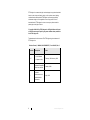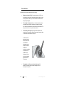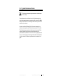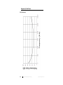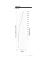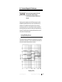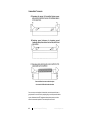
1
Model 7405 Near-Field Probe Set User Manual ETS-Lindgren Inc. reserves the right to make changes to any product described herein in order to improve function, design, or for any other reason. Nothing contained herein shall constitute ETS-Lindgren Inc. assuming any liability whatsoever arising out of the application or use of any product or circuit described herein. ETS-Lindgren Inc. does not convey any license under its patent rights or the rights of others. © Copyright 1996–2013 by ETS-Lindgren Inc. All Rights Reserved. No part of this document may be copied by any means without written permission from ETS-Lindgren Inc. Trademarks used in this document: The ETS-Lindgren logo is a trademark of ETS-Lindgren Inc. Revision Record | MANUAL,7405 PROBE SET | Part #399107, Rev. G Revision Description Date Initial Release A–E ii Updates / edits February, 1996–January, 1999 F Updated Preamplifier Gain chart; rebrand October, 2009 G Updated measurement and characterization information May, 2013 www.ets-lindgren.com Table of Contents Notes, Cautions, and Warnings ................................................ v 1.0 Introduction .......................................................................... 7 Magnetic (H) Field Probes .......................................................................... 8 Electric (E) Field Probes ............................................................................. 8 Ball Probe ........................................................................................... 9 Stub Probe.......................................................................................... 9 Standard Configuration ............................................................................... 9 Optional Items .......................................................................................... 10 ETS-Lindgren Product Information Bulletin ............................................... 10 2.0 Maintenance ....................................................................... 11 Service Procedures .................................................................................. 11 3.0 Electrical Specifications ................................................... 13 Model 7405 ............................................................................................... 13 Preamplifier .............................................................................................. 13 4.0 Operation ............................................................................ 15 Typical Configuration ................................................................................ 15 Probe Selection ........................................................................................ 16 Preamplifier Use ....................................................................................... 17 5.0 Typical Performance Factors ........................................... 19 Magnetic (H) Field Probes ........................................................................ 20 901 (6-cm Loop) ............................................................................... 20 902 (3-cm Loop) ............................................................................... 21 903 (1-cm Loop) ............................................................................... 22 Electric (E) Field Probes ........................................................................... 23 904 (Ball Probe) ................................................................................ 23 905 (Stub Probe) .............................................................................. 24 Preamplifier Gain ...................................................................................... 25 0.01 MHz –3 GHz ............................................................................. 25 6.0 Common Diagnostic Techniques ..................................... 27 Locating Radiating Sources ...................................................................... 27 Signal Demodulation ......................................................................... 29 www.ets-lindgren.com iii Examples .......................................................................................... 30 Using Sniffer Probes ......................................................................... 32 Diagnosing Radiation Causes ................................................................... 33 Common and Differential Mode Current Flow.................................... 35 Differential Mode Techniques............................................................ 40 Common Mode Techniques .............................................................. 42 Pre-Screening Alternate Solutions ............................................................ 43 Evaluating Alternate Solutions .......................................................... 46 Appendix A: Warranty ............................................................. 49 Appendix B: EC Declaration of Conformity .......................... 51 iv www.ets-lindgren.com Notes, Cautions, and Warnings Note: Denotes helpful information intended to provide tips for better use of the product. Caution: Denotes a hazard. Failure to follow instructions could result in minor personal injury and/or property damage. Included text gives proper procedures. Warning: Denotes a hazard. Failure to follow instructions could result in SEVERE personal injury and/or property damage. Included text gives proper procedures. See the ETS-Lindgren Product Information Bulletin for safety, regulatory, and other product marking information. www.ets-lindgren.com v This page intentionally left blank. vi www.ets-lindgren.com 1.0 Introduction The ETS-Lindgren Model 7405 Near-Field Probe Set includes three magnetic (H) field and two electric (E) field passive, near-field probes designed for use in the resolution of emissions problems. The Model 7405 provides a self-contained means of accurately detecting H-field and E-field emissions, and includes a 20 cm extension handle to provide access to remote areas in larger units. Made of injection molded industrial grade plastic, the probes are durable, light weight, and compact. The probes provide a fast and easy means of detecting and identifying signal sources that could prevent a product from meeting federal regulatory requirements. This set is a convenient and inexpensive tool for extending the capability of a spectrum analyzer, oscilloscope, or signal generator. A near-field probe is an essential tool for quick and efficient EMC/EMI engineering. Using near-field probes and an oscilloscope can produce the following results: Gain information about the source and location of the radiation member. Reduce test expense by adding inexpensive equipment for solving EMC/EMI problems. Reduce test time by pre-screening various solutions and alternate implementations. The Model 7405 is used for diagnostics purposes, and does not require calibration. www.ets-lindgren.com Introduction 7 Magnetic (H) Field Probes The Model 7405 includes three H-field probes of varying size and sensitivity: models 901, 902, and 903. These probes are highly selective of the H-field while being relatively immune to the E-field. Each H-field probe contains a single turn, shorted loop inside a balanced E-field shield. The loops are constructed by taking a single piece of 50 ohm, semi-rigid coax from the connector and turning it into a loop. When the end of the coax meets the shaft of the probe, both the center conductor and the shield are 360 degrees soldered to the shield at the shaft. Then a notch is cut at the high point of the loop. This notch creates a balanced E-field shield of the coax shield. The loops reject E-field signals due to the balanced shield. Electric (E) Field Probes The Model 7405 includes two E-field probes: the stub probe (model 904) and the ball probe (model 905). Due to the small sensing element, the stub probe is relatively insensitive. This is an advantage when the precise location of a radiating source must be determined. For example, while moving the stub probe over the pins of an IC chip, variations can be noted at spaces as close as two or three pins. By comparison, the ball probe is much more sensitive. The larger sensing element does not offer the highly-refined definition of the source location which the stub probe allows, but it is capable of tracing much weaker signals. The impedance of the stub probe is essentially the same as that of a non-terminated length of 50 ohm coaxial cable. 8 Introduction www.ets-lindgren.com BALL PROBE The shaft of the model 904 ball probe is constructed of a length of 50 ohm coax. The coax is terminated with a 50 ohm resistor in order to present a conjugate termination to the 50 ohm line. The center conductor is extended beyond the 50 ohm termination and attached to a 3.6-cm diameter metal ball, which serves as an E-field pick up. The absence of a closed loop prevents current flow, allowing the ball probe to reject the H-field. STUB PROBE The model 905 stub probe is made of a single piece of 50 ohm, semi-rigid coaxial cable with 6 mm of the center conductor exposed at the tip. This short length of center conductor serves as a monopole antenna to pick up E-field emanations. With no loop structure to carry current, the stub probe rejects the H-field. Standard Configuration H-field probes (3) E-field probes (2) 20 cm extension handle Carrying case www.ets-lindgren.com Introduction 9 Optional Items Preamplifier, including wall-mounted power supply (115 VAC or 230 VAC available) Preamplifier battery charger ETS-Lindgren Product Information Bulletin See the ETS-Lindgren Product Information Bulletin included with your shipment for the following: 10 Warranty information Safety, regulatory, and other product marking information Steps to receive your shipment Steps to return a component for service ETS-Lindgren calibration service ETS-Lindgren contact information Introduction www.ets-lindgren.com 2.0 Maintenance Before performing any maintenance, follow the safety information in the ETS-Lindgren Product Information Bulletin included with your shipment. WARRANTY Maintenance of the Model 7405 is limited to external components such as cables or connectors. If you have any questions concerning maintenance, contact ETS-Lindgren Customer Service. Service Procedures For the steps to return a system or system component to ETS-Lindgren for service, see the Product Information Bulletin included with your shipment. www.ets-lindgren.com Maintenance 11 This page intentionally left blank. 12 Maintenance www.ets-lindgren.com 3.0 Electrical Specifications Model 7405 Primary Sensor Type E/H or H/E Rejection Upper Resonant Frequency H-Field 41 dB 790 MHz H-Field 29 dB 1.5 GHz H-Field 11 dB 2.3 GHz E-Field 30 dB >1 GHz E-Field 30 dB >3 GHz 901 6-cm loop 902 3-cm loop 903 1-cm loop 904 3.6-cm ball 905 6-mm stub tip Preamplifier Absolute Maximum Ratings: Input Voltage (DC): 12 VDC Input Voltage (AC): +20 dBm Bandwidth: 100 kHz–3 GHz Noise Figure (Ref. 50 ohms): 3.5 dB (typical) Saturated Output Power (at F = 100 MHz): +12.0 dBm 1 dB Gain Compression (at F = 100 MHz): +10.0 dBm Third Order Intermodulation Intercept: +23 dBm www.ets-lindgren.com Electrical Specifications 13 This page intentionally left blank. 14 Electrical Specifications www.ets-lindgren.com 4.0 Operation Before connecting any components, follow the safety information in the ETS-Lindgren Product Information Bulletin included with your shipment. Typical Configuration 1. Choose the appropriate probe from the Model 7405 Near-Field Probe Set. See Probe Selection on page 16. 2. Connect a coaxial cable from the probe to the signal analyzing device; typically, an oscilloscope or spectrum analyzer. If needed, place the extension handle between the probe and the coaxial cable. 3. Adjust the signal analyzing device as required. www.ets-lindgren.com Operation 15 Probe Selection Choosing the correct probe is determined by the following: Whether the signal is E or H: If the signal is primarily is E-field, use the ball probe or stub probe. If the signal is primarily H-field, use one of the loop probes. If unknown, try one of each and select the one that best picks up the signal. The strength of the signal: Select a probe that adequately receives the desired signal of interest. Respectively, the ball probe and the 6-cm loop are the most sensitive of the E-field and H-field probes. The stub probe and the 1-cm loop are the least sensitive. The frequency of the signal: If the signal is above 790 MHz, the probe may go into resonance. See the upper resonant frequency listed for each probe in Specifications on page 13. In this illustration a ball probe is used to examine a flat cable. The distributed inductance over the length of the cables makes them particularly susceptible to common mode problems. High impedance sources such as this are best examined with an E-field probe. 16 The physical size of the space where the probe must fit: Model 7405 includes a variety of sizes. See pages 8–9 for a description of each probe. Operation www.ets-lindgren.com How closely you want to define the location of the source: Choose the probe that gets as close to the signal source as required. Select a large probe and begin outside a unit, then move closer to the source and switch to smaller probes to identify the location of the source. For example, the smallest probes should allow you to determine exactly which circuit on a printed circuit board is radiating. This kind of refinement provides the ability to stop the radiation at the source rather than shielding an entire unit. Preamplifier Use The optional preamplifier increases the sensitivity of your test system. The preamplifier is connected to the input of the signal analyzing device, and the coaxial cable from the probe is connected to the preamplifier. A switch on the preamplifier activates power to the unit; when power is activated, a panel light illuminates. The preamplifier is powered by a wall-mounted DC power supply. Both 115 VAC and 230 VAC models are available. The preamplifier includes a standard DC power connector. www.ets-lindgren.com Operation 17 This page intentionally left blank. 18 Operation www.ets-lindgren.com 5.0 Typical Performance Factors The following graphs represent typical measurement. Individual probe results may vary. Probe performance factor is defined as the ratio of the field presented to the probe to the voltage developed by the probe at the BNC connector, PF = EN. By adding the performance factor to the voltage measured from the probe, the field amplitude may be obtained. All probes in the Model 7405 Near-Field Probe Set were characterized in a transverse electromagnetic mode (TEM) cell which presented a 377 ohm field. The H-field probes only respond to the H-field; however, the equivalent E-field response is graphed. This may be done if the field is assumed to be a plane wave with an impedance of 377 ohms. The reason for graphing the factors this way is to allow estimation of the strength of the far-field. If H-field amplitude is desired, subtract 51.52 dB from the performance factor as indicated on the graph. www.ets-lindgren.com Typical Performance Factors 19 Magnetic (H) Field Probes 901 (6-CM LOOP) 20 Typical Performance Factors www.ets-lindgren.com 902 (3-CM LOOP) www.ets-lindgren.com Typical Performance Factors 21 903 (1-CM LOOP) 22 Typical Performance Factors www.ets-lindgren.com Electric (E) Field Probes 904 (BALL PROBE) www.ets-lindgren.com Typical Performance Factors 23 905 (STUB PROBE) 24 Typical Performance Factors www.ets-lindgren.com Preamplifier Gain 0.01 MHZ –3 GHZ www.ets-lindgren.com Typical Performance Factors 25 This page intentionally left blank. 26 Typical Performance Factors www.ets-lindgren.com 6.0 Common Diagnostic Techniques Before connecting any components, follow the safety information in the ETS-Lindgren Product Information Bulletin included with your shipment. Obtaining accurate, repeatable results from EMI testing requires a carefully established and characterized test setup, usually an open field test site or a shielded room. Final qualification must be performed in the required test environment of a screen room or an open field site. However, a great deal of preliminary EMI testing can be done with a sniffer probe and signal analyzing instrument. The following sections describe how sniffer probes can be used in various phases of the engineering task. Locating Radiating Sources The first step is to relate the emissions failure to signals used in the Equipment Under Test (EUT) being tested. To do this an understanding of the nature of the time domain to frequency domain transform is necessary. www.ets-lindgren.com Common Diagnostic Techniques 27 The various specifications are given in the frequency domain, so there are many dBuV at a particular bandwidth over a given frequency range. However, most EUT operations are characterized in the time domain: 150 ns memory access time, 300 V/ms slew rate, and so on. This section presents a technique that will aid in linking emissions with the signals that create them. During testing you may receive information indicating, for example, that it failed by 10 dB at 40 MHz and 3 dB at 120 MHz. The challenge is to find the EUT function that created the emissions. You may be able to connect the probe to a spectrum analyzer and locate the source; locating the source of an emanating signal begins by finding the exit points. Cover seams and air flow vent holes are primary suspects. However, many sources can emit at a given frequency. Most of these emissions are non-propagating, reactive fields. The most helpful first step in locating the sources of a propagating field is to demodulate the offending signal while it is being received in the far-field. Demodulation gives a time domain representation of the signal. This time domain representation will appear in some way similar to an oscilloscope trace of the radiating signal. 28 Common Diagnostic Techniques www.ets-lindgren.com SIGNAL DEMODULATION To demodulate a signal: 1. Set the spectrum analyzer for a 0 Hz frequency span and tune to the signal of interest. This essentially changes the spectrum analyzer into a tuned receiver and makes the display a frequency filtered oscilloscope. 2. Take the video output off the spectrum analyzer and run it to the oscilloscope. Using the oscilloscope as the display allows greater flexibility in adjusting the signal amplitude and in triggering. www.ets-lindgren.com Common Diagnostic Techniques 29 3. Obtain a clear picture of the signal produced on the oscilloscope. You now have a good representation of what you are looking for when you start sniffing with the probe. Produce scope photos of the demodulated trouble frequencies and then use the sniffer probes to look for similar signals in your equipment. Locate close matches to the demodulated signals for clues to the source of these signals. When you find the sources you will determine the subassemblies, circuits, or gates that need work. There are several physical phenomena that cause lower frequency signals to modulate and radiate as high frequency signals. A working knowledge of FM, AM, audio rectification, and other phenomena provides greater ability to understand and interpret the data revealed by demodulated signals. This understanding gives insight into the kind of radiating structure that must be present to produce the observed event, and also allows greater facility in recognizing the original signal from the altered and often distorted, modulated representation. Frequently the demodulated picture will contain just the transitions of a digital signal. At times, only the rising or falling edge will be present in a high frequency signal. Understanding the radiation physics allows the appearance of the original signal to be surmised. Often all that will be present in the photograph from the oscilloscope presentation is the high frequency components of a signal. These waveform components are the source of the radiation. EXAMPLES Getting an idea of what the waveform may look like through demodulation is not the only use for the time domain-frequency domain transform. Analysis can reveal the component of the waveform that is causing the problem. Example: 30 If you have a 16 MHz clock and you have a 16 MHz problem, then you know that the base signal is causing the problem. More typically, your probing may lead you to the 16 MHz clock when trying to find the 208 MHz problem. Remember a 208 MHz signal has a wavelength of 1/13 of 16 MHz. Common Diagnostic Techniques www.ets-lindgren.com If the problem is caused by a rise or fall time, you may be looking for a waveform component which is between a wavelength and 1/8 of a wavelength of the radiating frequency. Example: In the 208 MHz example a wavelength is 1/13 of the 16 MHz clock; 1/8 of a wavelength is 1/104 of a 16 MHz pulse width. Look at the oscilloscope picture for waveform components on the 16 MHz clock that are 1/13–1/104 of the 16 MHz wavelength. You can then begin to zero in on undershoot and overshoot or other parasitic components. You may not have to quiet the entire circuit, but rather roll off the offending components. What you have done is mentally transform a frequency domain failure to a time domain picture that you can work on. After identifying what the signal of interest looks like on the oscilloscope, it must be located within the equipment. At times this will have already been accomplished during the demodulation process. Example: As you demodulated a 5 MHz signal, maybe it became clear that the 50 MHz was pulsing on at a 40 kHz rate. You may know that the only 40 kHz source in your unit is the switching rate in the power supply. If nothing else in the unit operates at that frequency, you have identified your source. Thus, the first step in identifying a signal source is to review what subassemblies in the unit may produce a signal similar to the one you are seeing radiated. www.ets-lindgren.com Common Diagnostic Techniques 31 USING SNIFFER PROBES Typically, there are several possible sources for a given signal. To identify the particular one in question, use the sniffer probes. 1. From a set of loop probes of varying sizes, start with the largest, which is also the most sensitive. Begin several feet from the unit and look at the signal of interest. Search for the maximum and approach the unit along the line of maximum emission. 2. As you near the unit, switch to the next smaller probe; this probe will be less sensitive but will differentiate the signal source more narrowly. Often the initial probing locates where the signal is escaping from the unit, indicating the point of escape from the housing. 3. Once inside the unit and inside any shielding, look for the source of the signal; use the smallest diameter probe available. You may switch to the stub probe, which is a small and insensitive E-field probe that can be used to get close to the signal source. Finding both the point of escape from the unit and the actual source provides choice in engineering the solution: you may decide to improve the shielding or to suppress the source. The more solution alternatives you identify the greater the chance of identifying one which meets all the requirements of schedule, cost, and performance. Another procedure is to use electromagnetic probes in conjunction with regular scope probes. 1. Connect a regular scope probe and switch back and forth to refine the offending components as finely as possible. Using this combination can define a radiating source to a specific signal line. 2. Periodically disable portions of a circuit to make a final determination of the location of the source. For example, disable a line driver to see if the radiation is coming from the base unit or from a cable. When disabling parts of a circuit, use a sensitive probe and take readings several meters from the unit. Clear the scope probe out of the unit when making radiated readings; an attached scope probe can easily radiate and mask the real problem. When done, you should have a good idea of the exact location of the offending signal. 32 Common Diagnostic Techniques www.ets-lindgren.com Diagnosing Radiation Causes A small sniffer probe can help diagnose the cause of an electromagnetic interference problem. This section addresses using sniffer probes for a rough estimate of field impedance, which is used to diagnose the radiation physics of a given situation. Knowing the field impedance can help find solutions to EMI problems. When presented with an EMC/EMI problem, you need to know two things: 1) What is radiating inside the unit, and 2) Why the component or circuit is radiating. www.ets-lindgren.com Common Diagnostic Techniques 33 Radiation is caused by an instantaneous change in current flow, causing a magnetic field, or by an instantaneous change of a potential difference, causing an electric field. Experience has shown a high degree of correlation between magnetic fields with differential mode current flow. Although a change in voltage will cause a change in current and vice versa, one of these vectors will predominate. The impedance of the radiating source will determine whether a predominately magnetic or predominately electric field is produced. Typically, magnetic fields are produced by local current loops within a unit. These loops may be analyzed as differential mode. Electric fields require high-impedance sources. Because the changing potential is isolated by substantial impedance on all lines into the circuit, all lines will carry just the forward current. The impedance in this context is the total impedance at the radiating frequency. Often what appears as low-impedance connections are actually high-impedance due to the inductance in the physical circuit. A common way for all lines in a circuit to become high-impedance lines is for the ground servicing that circuit to contain a significant inductance. At some frequency, this ground inductance becomes a high-impedance. Because the entire circuit references ground, this impedance in the ground path effectively is in series with every line in the circuit. The return flow in this situation is developed by capacitive coupling to conductors external to the unit or to fortuitous conductors within the unit. 34 Common Diagnostic Techniques www.ets-lindgren.com COMMON AND DIFFERENTIAL MODE CURRENT FLOW From the local perspective of the unit, this is a common mode situation; EMC/EMI problems may be classified principally as current-related or voltage-related. Current-related problems are normally associated with differential mode situations. Likewise, voltage problems are normally associated with common mode circuit situations. Too often solutions are attempted before the radiating parameter is understood. Unfortunately, solutions effective for differential mode are seldom effective against a common mode problem. www.ets-lindgren.com Common Diagnostic Techniques 35 To review the physics of the situation: In a far-field that is more than about one wavelength from the source, the ratio of the E-field and H-field components to the propagating wave resolve themselves to the free space impedance of 377 ohms. In the far-field the E-field and H-field vectors will always have a ratio of 377 ohms, but in the near-field that ratio radically changes. The ratio of E-field to H-field, or field impedance, is determined in the near-field by the source impedance. As you probe close to the equipment you can switch between an E-field probe and an H-field probe. By noting the rate of change of the field strength versus distance from the source and the relative amplitude measured by the probes, the relative field impedance may be determined. Low-impedance sources or current-generated fields initially will have predominately magnetic fields. The magnetic component of the field will predominate in the near-field but will display a rapid fall-off as you move away from the unit. This change may be observed through an H-field probe. Low-impedance sources also will give a higher reading in the near-field on an H-field probe than on an E-field probe. Alternately, high impedance sources will display a rapid fall-off when observed through an E-field probe. There are two ways to determine the nature and source impedance: Map the rate of fall-off of the E-field and H-field. One of these vectors will fall off more rapidly that the other. Measure both vectors at the same point and by their ratio determine the field impedance. The equation E/H=Z is calculated and compared to the free space impedance of 377 ohms. Values higher than 377 ohms will indicate a predominance of the electric field. Lower values will indicate that the magnetic field component is predomination. From this you can plan your approach to the problem by tailoring it to a differential model situation or a common mode situation. Field theory leads us to expect a 1/R fall-off for a plane wave, where R is the distance from the source. In the near-field, the non-propagating, reactive field will drop off at multiple powers of the inverse of the distance 1/RN. Typically, the reactive field will fall off at something approaching 1/R3. Therefore, we would predict these measurements relative to measurements at distance equal to one. 36 Common Diagnostic Techniques www.ets-lindgren.com Distance: A to B = 1.5 2.0 3.0 Propagating Field: 1/R –3.52 dB –6.02 dB –9.54 dB Reactive Field: 1/R –10.57 dB –18.06 dB –28.63 dB 3 After the source is identified, two or three angles of approach are measured. A typical situation would record two points at 0.5 meters and 1.5 meters from the source along two radials from the source. The signal is measured at each point with a probe which is highly selective of the H-field and another probe which is highly selective of the E-field. The rate of fall-off is noted for each probe and the relative amplitude between the probes is noted. In deciding what the relative amplitude is, the conversion factor of each probe must be taken into account. www.ets-lindgren.com Common Diagnostic Techniques 37 38 Differential mode data is generally well behaved. The amplitude measured with the H-field probe will be significantly higher than that measurement with the E-field probe. Also, the H-field will drop off at a much faster rate than the E-field. Common mode measurements are generally less well behaved. Often the best indicator is the relative amplitude. The E-field probe will have a much higher reading than the H-field probe. The drop-off rate will be faster when measured with the E-field probe. However, experience shows that the E-field, being a high potential field, is much more susceptible to perturbation. Often the reading will be sensitive to cable placement and differences in the position of the person holding the probe. This susceptibility to being perturbed can be a hint that the field is coming from a high potential source. Common Diagnostic Techniques www.ets-lindgren.com A qualitative knowledge of the field impedance indicates how to approach the EMC/EMI design for the problem. By determining the dynamics of the radiating structure, it can be surmised what kinds of designs will be effective is solving the radiation problem. A primarily H-field problem signifies that current flow predominates. The other possibility is that the problem is predominately electrical or E-field. In this case the field impedance is relatively high. A high field impedance means there is a potential build-up across some impedance, and this high potential region is the radiating source. A differential mode problem will respond to these types of remedies: Reducing circuit loop area. Reducing signal voltage swing. Shielding the entire radiating loop. It will not respond well to partial shielding of the radiating loop. Partial shielding typically occurs when the path of the return current is mapped incorrectly and not included inside the shield. Filtering the radiating signal line. www.ets-lindgren.com Common Diagnostic Techniques 39 DIFFERENTIAL MODE TECHNIQUES Some traditional differential mode techniques do not work in common mode situations When differential mode solutions are applied to a common mode problem; many of the techniques will prove ineffective. For example: 40 Reducing circuit loop area: The radiating signal is on the signal and return path, so this will be ineffective. Using twisted pair wires or coax will yield little in the way of signal reduction. Common Diagnostic Techniques www.ets-lindgren.com Reducing the signal voltage swing: This will be ineffective when the radiating potential is developed deep in the circuitry, not at the output signal driver. At times the radiating potential will be built up on the power or ground system through the additive effects of a number of gates. Therefore, suppression of any one of these gates in isolation will not yield much signal reduction. Shielding the entire loop: A problem arises when deciding where to ground the shield. The radiating potential is on signal ground, but if you tie the shield to signal ground, you ultimately add more radiating antenna to the system. Filtering the signal line: A problem arises when deciding where to ground the filter. Using signal ground will be ineffective because the filter will float with the radiating potential. www.ets-lindgren.com Common Diagnostic Techniques 41 COMMON MODE TECHNIQUES Some traditional common mode techniques do not work in differential mode situations Once a common mode problem is determined, use techniques which have a good potential for success. Start by analyzing the ground and power distribution system. Understand what RF impedances these systems present, and then reduce the excessive impedance. These techniques can be tried: 42 Common Diagnostic Techniques www.ets-lindgren.com Increasing decoupling of power to ground. Reduce lead or trace inductance by reducing their length or making them wider. Inserting ground and power grids or planes. Shielding, using a ground separate from signal ground. Relocating I/O cables to a lower impedance area on the ground structure. Placing common mode filters on the output lines using dissipating elements. Pre-Screening Alternate Solutions Pre-screening allows you to sort through ideas, formulate test plans, and take several viable solutions to the range. Pre-screening also provides empirical evidence that a noise reduction technique has been correctly applied, and indicates when you have properly analyzed the problem to the point of designing an effective solution. Testing alternate solutions can save time when troubleshooting an electromagnetic problem. For example, for a common mode problem that involves radiation from the end of a unit with the I/O connections, possible solutions could include the following: Improve the decoupling on the board. Improve the power and ground grading or put in a ground plane. Decouple the end with the I/O connections to chassis ground. Place a common model choke on the output I/O. The most economical solution may be a hybrid of these options applied in conjunction. Each option could be implemented a number of ways, and the physical mechanization of an approach will directly impact overall effectiveness. www.ets-lindgren.com Common Diagnostic Techniques 43 Evaluating various solutions requires great skill and awareness, and it is in this area that the far-field/near-field effects can be the most misleading. The E-field and H-field vectors are initially determined by the source impedance. As you move away from the source, these vectors increasingly balance until the radiating field is isolated as a plane wave with a characteristic impedance of 377 ohms. In the near-field the field strength can contain, in addition to the radiating field, a significant non-radiating reactive component. This reactive component does not propagate far. The radiating field will fall off proportionally with the reciprocal of the first power of the distance from the source, 1/R. However, the reactive component will fall off proportionate with the reciprocal of multiple powers of the distance from the source, 1/RN. 3 Typically, the reactive field will fall off at a rate approaching 1/R . Two points should be observed: 1. Often the near-field reading will be dramatically different than would be expected based on an extrapolation of the far-field reading. Near-field readings will seem higher than expected due to the presence of the reactive field; alternately, it may be lower than expected because of nulls created by the interference pattern set up near the unit. A reflection pattern is often established near the unit by the direct wave combining with the reflection off parts of the unit and other items in the vicinity. A design which reduces field strength by attenuating the non-radiating, reactive field may show relatively little effect on the far-field reading. 44 Common Diagnostic Techniques www.ets-lindgren.com 2. The probe becomes part of the circuit during near-field measurements. There is capacitance and inductance between the circuit being measured and the probe with the associated cabling. The probe will re-radiate the received field, altering the field being measured. However, technical imprecision does not necessarily eliminate a method. Sometimes an attenuation of the field strength in the near-field will translate into an attenuation of the far-field reading. As long as a linear relationship is not expected, there can be real benefit from near-field probing. Generally, a reduction of the non-radiating field will also mean that the radiating field has been reduced. www.ets-lindgren.com Common Diagnostic Techniques 45 EVALUATING ALTERNATE SOLUTIONS There are two approaches that yield good results when evaluating alternate design solutions: 1. The first step in each procedure is to choose a set of points; for example, two to six points. Since the object is to determine what the far-field results will be, most of the points should be one to four meters away. Also, choose one or two points close to the source. If a solution results in a dramatic reduction, this point may be the only one that will allow quantitative measurement of the reduction. The placement of ground straps changes the geometry of the radiating current loop. A ground strap may reduce the signal, but it will also redirect it. To properly assess the modification, the perimeter of the unit must be scanned. 46 Common Diagnostic Techniques www.ets-lindgren.com The more distant measurement points may lose the signal into the system noise; a given solution may only redirect the beam. Especially with narrow beam problems, solutions frequently only shift the beam so that it radiates in a different direction. After measurement points are chosen, baseline the unit by measuring each point with an E-field and an H-field probe. That way, each design alternative can be implemented and measured over the same set of points. 2. The two procedures differ here in how they approach the measurements that have been taken. The first method is based upon finding a solution with a large safety margin. For example, suppose a signal fails the required limit by 3 dB. Once that signal is found in the lab, it can be measured in the near-field. The goal is then to reduce in this near-field the 3 dB plus a safety factor of 6 dB or 10 dB. This allows a large margin of error due to near-field effects. Additionally, a solution that passes this must then be confirmed by far-field measurements. The second method identifies several solutions which could be effective. In the previous example where the signal failed by 3 dB, after pre-screening in the lab, a variety of solutions may be selected and tested. A final benefit of pre-screening is that through the inevitable failures, new information can be discovered. For example, an attempt to reduce an emission may fail the following reasons: 1. The diagnosis was wrong. 2. The technique was inappropriate to the diagnosis. www.ets-lindgren.com Common Diagnostic Techniques 47 3. The technique was improperly applied. 4. An outside factor is involved, such as a second source radiating at the same frequency. Example: A solution that worked in the lab and on the range before 10:00 AM failed later in the day. Analysis revealed that the rise in temperature was affecting the values of decoupling capacitors, making them less effective at higher temperatures. 48 Common Diagnostic Techniques www.ets-lindgren.com Appendix A: Warranty See the Product Information Bulletin included with your shipment for the complete ETS-Lindgren warranty for your Model 7405. DURATION OF WARRANTIES FOR MODEL 7405 All product warranties, except the warranty of title, and all remedies for warranty failures are limited to two years. Product Warranted Duration of Warranty Period Model 7405 Near-Field Probe Set 2 Years www.ets-lindgren.com Warranty 49 This page intentionally left blank. 50 Warranty www.ets-lindgren.com Appendix B: EC Declaration of Conformity www.ets-lindgren.com EC Declaration of Conformity 51