Download experience and techniques in modelling urban stormwater networks

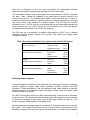
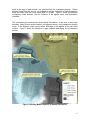
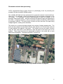
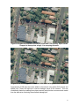
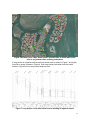
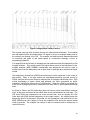
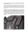
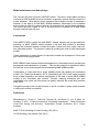
EXPERIENCE AND TECHNIQUES IN MODELLING URBAN
STORMWATER NETWORKS AND OVERLAND FLOW PATHS
S Cornelius1, H Mirfenderesk2, E Chong2
1
DHI Water & Environment Pty Ltd, Brisbane, QLD
Gold Coast City Council, Nerang, QLD
2
Abstract
Gold Coast City Council is developing coupled hydraulic models of the city using the
rainfall on grid method for use in asset management, risk assessment and city planning.
The current flood hazard maps used for planning were developed using two dimensional
hydraulic models (MIKE 21) with course grids and hydrological modelling undertaken using
URBS. The current approach does not simulate localised flooding and overland flow paths
away from the main river channels, or capture the interaction between the stormwater
network, overland flows, flood plains and river channels.
The Waterways and Flood Management Team have identified the need to account for this
interaction, particularly in planning for adaption to climate change. Thirteen percent
(approx. by pipe length) of the storm water network is in the intertidal zone. This is
estimated to increase to 20 percent by the year 2100 based on the IPCC medium scenario
prediction of an 80cm increase in sea level. This has implications for network capacity and
asset life. Climate change adaption policy options are being considered, and analysis
requires a consistent modelling approach across the city.
To improve confidence in modelling Council has decided to develop three way coupled
MIKE FLOOD models where MIKE21 is used for flood plains, overland flow paths, open
channels and rainfall runoff in a 2m grid. MIKE URBAN is used for pipe networks, and
MIKE11 for significant hydraulic structures.
This new approach has some significant challenges primarily related to data availability
and computing power. The stormwater network contains over 100,000 pipes for which
varying quality data is available. The 2m grid of the city contains over 590 million grid cells.
In order to keep model domains reasonable the city will be divided into approximately 300+
drainage models. DHI have worked with Council to develop tools for managing the network
data and model building process. The model data management and model building
process are the main focus of this paper.
Introduction
The Gold Coast is located in South-East Queensland, Australia. The city’s landscape
consists of steep valleys in the West which drain into broad coastal flood plains in the
East. Urban development, including the construction of extensive navigable canal
networks, is concentrated on the low lying coastal areas. Flood risks arise from riverine
flooding, storm tide, storm water network capacity, and flash flooding in the steep upper
catchments.
1
The Waterways and Flood Management (WFM) Team at the Gold Coast City Council
(GCCC) provide flood modelling services to the GCCC. The WFM have identified the need
to accurately model the interaction between overland flow paths, creeks and rivers, canals,
sea level, and stormwater assets. These models need to be developed to a consistent
standard across the city to enable policy to be determined at a city wide scale. The models
also need to be complete enough to be used for detail design and need to be able to
accurately represent the operation of pumps and controlled weirs.
Modelling approach
Historically, the WFM has been an early adopter of modelling technology, initially using
one dimensional (1D) hydraulic models such as MIKE11 with URBS hydrological models
for analysis of river flooding and storm surge. More recently, two dimensional (2D)
hydrodynamic models of rivers and floodplains, such as MIKE 21 have been developed
using course grids. These also use URBS for hydrological modelling.
2D models can provide better representation of the flood plains and overland flow paths
than 1D models which are more suited to river channels. The URBS models developed
use relatively large catchments and the resulting discharge hydrographs are applied to the
main channels in the 1D and 2D models. When used in this manner, the models do not
provide an accurate representation of overland flow and ponding away from the main river
channels.
WFM are now using a nested 1D – 2D model which allows MIKE URBAN, MIKE11 and
MIKE21 models to be dynamically coupled. This approach allows the stormwater network
including complex hydraulic structures to be modelled along with the rivers, canals, and
flood plains. This enables the interaction between the stormwater system and the main
channels to be represented.
Much finer grids are being used in the 2D models improving the representation of overland
flows.
Hydrology is now being undertaken directly in the 2D models using the rain on grid
approach. This allows overland flow paths and ponding away from the main channels to
be represented in the model. This also removes the need to build and run separate
hydrological models, which can be a time consuming process if catchments are delineated
for each entry point to the piped network.
Challenges
Building nested 1D – 2D models using the rain on grid approach is relatively quickly and
easy, with a comprehensive suite of tools available in the MIKE software. However the
size of the study area (approximately 2,400km2, or 590 million 2m x 2m grid cells) and the
large number of stormwater network features creates some model building and data
management challenges.
Computing power available to WFM limits the size of the bathymetry and roughness grids
used in MIKE21 modelling to around three million elements. This effectively limits model
domains to 12km2. The flat topography on the flood plains in Gold Coast does not readily
2
lend itself to delineation of the real world watersheds into manageable domains,
furthermore stormwater networks often cross the water shed boundaries.
The stormwater networks used in the models are primarily based on GCCC’s corporate
GIS data. Table 1 shows the availability of key model data for assets included in the
councils GIS data set. The available data contains errors and there are a number of
assets not included in the dataset. Typically manhole lid levels and depths do not correlate
well to the inverts levels available for connected pipes. The GIS data also contains
digitisation errors. The GIS data can be supplemented with as constructed drawings and
survey; however the use of this is limited by cost. Consequently the GIS data requires
considerable clean up before it can be used for modelling.
The GIS data set is maintained by separate departments at GCCC and is updated
frequently, requiring periodic updates to the models. This creates an on-going model
maintenance issues.
Table 1 Percentage availability of key network data in GCCC GIS data set
Links
(115,171 polylines)
Drainage Pits
(79,769 Points and Polygons)
Outlets
(12,624 Points and Polygons)
Chambers
(28,690 Points and Polygons)
Diameter
Upstream Invert
Downstream Invert
Lid Level
Invert level
Depth
Diameter/Area
Lid Level
Invert level
Depth
99.8%
40.1%
59.8%
60.1%
0.0%
60.1%
29.7%
66.0%
0.0%
3.8%
Lid Level
Depth
Invert level
Diameter/Area
60.4%
60.3%
0.0%
12.0%
Stitching models together
As model domains are typically of sub catchment scale a process of stitching overlapping
domains together at logical depth and/or discharge boundary locations has been
employed. Careful delineation of the sub catchment scale model domains is required,
taking the location of overland flow paths, stormwater network, rivers and canals, model
domain limitations into account.
The ARC GIS Hydrology toolbox has been used extensively in the process of delineating
model domains. This ensures that domain extents align with ridgelines and that sinks are
not present at the edge of the domain, which would cause flooding on ridge line in the
model, resulting in model stability and mapping issues.
Model domains are overlapped where it is necessary to connect domains at rivers, creeks,
and canals. The overlap is made large enough to ensure that any interference from the
boundary is outside of the study area extent for each domain. The water level boundaries
3
used at the edge of each domain, are extracted from the overlapping domain. Where
adjacent model domains are not yet available to provide discharge or depth boundaries
these are taken from the course scale MIKE 21 models. Figure 1 shows two adjacent
overlapping model domains, with the locations of the applied water level boundaries
indicated.
The stormwater pipe networks also cross domain boundaries. In this case a water level
boundary, taken from the outlet location in the adjacent domain, can be applied to the pipe
outlet. In the adjacent model a point source discharge is also applied at the pipe outlet
location. Figure 1 shows an example of a pipe networks discharging into the adjacent
domain.
Figure 1 Stitching Models together at domain boundaries.
4
Stormwater network data processing
GCCC commissioned DHI to assist Council in by developing a tool for processing the
available GIS data into MIKE URBAN models.
The available GIS data has been processed into a geometric network of points and lines.
There are 1,150 manholes, outlets and drainage pits that are stored as polygons in the
GIS system. It is necessary to convert these polygons to points for inclusion in the
geometric network and model. As these structures are relatively large, the biggest being
over 90m2, a snapping tolerance (~10m) is required to achieve connectivity when building
the geometric network. This would result in points and lines less than 10m apart being
snapped together, creating errors elsewhere.
The solution is to convert the large polygons into a series of closely spaced points. The
pipes are then snapped to these points using a snap tolerance of 0.3m and from node and
to node attributes are applied to the pipes. The network can then be rebuilt, this time
using the from node and to node attribute to snap the pipes to the centre point of the
polygon. These large structures are represented as basins in the model with an area
taken from the polygons. The steps are shown in Figure 2 to 4.
Figure 2 Raw GIS data with large chambers stored as polygons
5
Figure 3 Polygons boundaries converted to points with 0.1m spacing. Pipes can be
snapped to these points using a 0.1m snapping tolerance.
Figure 4 The resulting geometric network with basins at large structure locations.
Approximately 5,000 pipes were also added to the network using similar GIS routines and
spatial joins. These are required to connect drainage sumps to the network. This was
considerably faster than adding these pipes manually and provides a more accurate model
than the alternative of deleting disconnected drainage pits.
6
The resulting geometric network is being stored in a master database on GCCC’s server.
The network data for each model can be downloaded to a MIKE URBAN database on the
modeller’s machine.
The tool processes the level and diameter data for the pipes, manholes, inlets, outlets and
drainage pits in the local MIKE URBAN database. The tool interpolates and estimates
missing data based on available data and design standards then performs a series of
sanity checks. The process removes almost all errors that would prevent the model from
running before populating all required fields in the MIKE URBAN database, and
symbolising critical and non-critical errors graphically in MIKE URBAN. Non-critical errors
will not prevent the model from running but should be fixed to improve model accuracy.
Figure 5 shows the network for the Runaway Bay model prior to any manual clean-up
effort being undertaken. Although the network contains 2,385 nodes, and 2139 links there
are only 12 critical errors in the data, symbolised by the large red circles. Non-critical
errors are symbolised by the smaller green circles.
The removal of errors and symbolisation of remaining errors significantly reduces the
manual effort required by the modeller to clean up the network. Typically the time required
to clean up the network data for a model is in the order of hours rather than weeks. Figure
6 shows a model with critical and non-critical errors symbolised before any manual cleanup has been undertaken. In this instance there is a single critical error shown in red near
the middle of the model. The green circles are non-critical errors where the pipes are
larger than 600mm diameter, and the blue circles are non-critical errors on smaller pipe
lines.
7
Figure 5 Runaway Bay model, symbolization of model data errors prior to any
manual clean up being undertaken.
8
Figure 6 Paradise Point, Hope Island model, symbolisation of model data errors
prior to any manual clean up being undertaken.
A long section of a pipeline with several non-critical errors is shown in Figure 7 and a pipe
line with no errors is shown in Figure 8. Both long sections are taken from the model
shown in Figure 6 prior to any manual clean-up work.
Figure 7 Long section 1 with non-critical errors resulting in negative slopes.
9
Figure 8 Long section 2 with no errors
The manual clean-up effort involves cleaning the network and bathymetry. The modeller
can add additional links and nodes where it is logical to do so, for example where parts of
the network are missing in the GIS. The modeller can add level and diameter/area data
for manholes and pipes to the model based on construction drawings, survey, or
engineering judgement.
It is essential that the lid levels of drainage pits and manholes match the bathymetry at the
coupled locations. Pipe outlets need to be higher than or equal to the bathymetry at the
coupled locations. MIKE URBAN’s interpolation and assignment tool can be used to
extract levels from the bathymetry and to apply them to drainage pits, manholes and pipe
outlets.
The bathymetry, derived from LiDAR and boat surveys is often inaccurate in the vicinity of
pipe outlets. Many of the pipe outlets are submerged preventing accurate survey by
LiDAR, and boat surveys are limited to deeper parts of navigable canals and rivers. Pipe
outlets discharging to opens drains and wetlands are often surrounded by dense
vegetation, which limits the accuracy of LiDAR survey. When the LiDAR is processed into
a 2m grid an averaging process is employed which may result in small open drains being
filled.
As shown in Table 1 the GIS outlets layer does not have an invert level attribute, however
many of the pipes connected to the outlets have invert level attributes for both ends. The
GIS invert levels are considered to be more accurate than, and are typically 0.1-0.5m
lower than the LiDAR derived bathymetry at the couple location. As coupling below the
bathymetry level is not allowed in the model, the tool symbolises a non-critical error in the
MIKE URBAN map view, helping to focus the modeller’s effort during the manual model
clean-up process. The modeller can choose to edit the network levels or bathymetry to
resolve this error.
10
As the modeller adds data to the model, the tool updates data that is interpolated or
estimated based on design standards, updates the model and updates the symbolisation
of errors in the map view.
The tool tracks the origin of all data used in the model. This is necessary as the models
may be used by other departments for detail design of upgrades to the stormwater
network. Typically assets are surveyed during detail design, if there is any doubt as to the
accuracy of the data. This survey effort can be greatly reduced if the source of the data is
available. The date, time and the current logged in user name is stored for all data added
to the model.
Figure 9 shows a model network and bathymetry after manual clean-up has been
completed and all critical and non-critical errors have been resolved. The tool also sets
default values for all fields in the MIKE URBAN database where a value has not been
provided by the modeller. For example the pressure main field in the links table is set to
false, and the formulation for links is set to Mannings Explicit except at outlets where it is
set to Mannings Implicit to improve model stability. As much of the data used in the final
model is interpolated or estimated based on design standards, it is likely that the model
network is not a perfect representation of the real system. However the model has been
developed to a very high standard, using the limited available data and is well
documented.
Figure 9 Paradise Point Hope Island model network and bathymetry after manual
clean-up.
11
Model maintenance and data storage
The Councils GIS data is stored in MAPINFO tables. The data in these tables are being
converted to ESRI shapefile format, processed in a geometric network and then stored in a
master database. When starting a new catchment the modellers are able to download a
selection of this data to a local MIKE URBAN database. Subsequent to the modellers
manual clean-up effort the network data can be imported back into the Master database.
The current date time, logged in user id, and data source is available for all data added
during the manual clean-up work.
Conclusions
Using MIKE FLOOD to couple fine scale MIKE21 models, using the rain on grid method for
hydrology, to MIKE URBAN models provides a fast and easy method to accurately
simulate the interaction between overland flow paths, creeks and rivers, canals, sea level,
and stormwater assets. This process is eased by avoiding the need to build hydrological
models.
Careful delineation of model domains is required to enable the development of fine scale
grid models covering large areas.
MIKE URBAN’s open framework allows development of customised tools for managing the
development and maintenance of models. This has the potential to significantly reduce
the time and survey costs required to build and debug MIKE URBAN models.
Centralisation of model data into a single database helps with building and maintaining
models. The Toolbox developed by DHI in collaboration with GCCC has saved countless
hours of data preparation and manual manipulation of GIS data to create MIKE URBAN
models of the stormwater pipe network. Thematic mapping techniques and error
classification into critical and non-critical has greatly improved the model build workflow
within WFM.
Though the concept of rain on grid has been in use for a number of years, further research
in refining this method is warranted.
References
Mirfenderesk, H., Chong, E., Tonks, M., Rahman, M., Van Doorn, R., Vis, S., Kabir, M.,
Cornelius, S. 2011. ‘Coastal Infrastructure Vulnerability Assessment – Trade-Off between
Coast-Time Saving and Accuracy’, Queensland Coastal Conference 2011, Cairns,
Australia.
MIKE FLOOD: Modelling of Urban Flooding, DHI (2011).
1D-2D Modelling: User Manual, DHI (2011).
12