Download Using the MSC121x as a High-Precision Intelligent Temperature

Application Report
SBAA100 - July 2003
Using the MSC121x as a High-Precision Intelligent
Temperature Sensor
Hugo Cheung
Data Acquisition Products − Microsystems
ABSTRACT
The MSC121x [1] is an embedded controller with a high-precision, high-stability temperature
sensor, a 24-bit delta-sigma (∆Σ) analog-to-digital converter (ADC), and an enhanced 8051
CPU. These circuit functions are the major building blocks for an intelligent temperature
sensor. After temperature calibration, the on-chip temperature sensor measurement
accuracy can reach ±0.1°C with a resolution of 0.01°C over an operating range of –40°C to
85°C. Applications for precision temperature measurements include, but are not limited to,
thermocouple cold-junction-correction measurement, industrial process control, and system
temperature monitoring. This article introduces the fundamental concept and operation of the
on-chip temperature sensor. This report also describes the calibration procedures to turn the
device into a high precision intelligent temperature sensor.
This application note uses the term MSC121x to refer to the MSC1210/MSC1211/MSC1212
as a series of devices.
Contents
Temperature Sensing System . . . . . . . . . . . . . . . . . . . . . . . . . . . . . . . . . . . . . . . . . . . . . . . . . . . . . . . . 2
1.1 Temperature Sensor Circuit . . . . . . . . . . . . . . . . . . . . . . . . . . . . . . . . . . . . . . . . . . . . . . . . . . . . . . . 3
1.2 Temperature Sensor Parameters . . . . . . . . . . . . . . . . . . . . . . . . . . . . . . . . . . . . . . . . . . . . . . . . . . 4
1.3 Ideal Diode Equation . . . . . . . . . . . . . . . . . . . . . . . . . . . . . . . . . . . . . . . . . . . . . . . . . . . . . . . . . . . . . 5
2
Temperature Sensor Accuracy . . . . . . . . . . . . . . . . . . . . . . . . . . . . . . . . . . . . . . . . . . . . . . . . . . . . . . . 6
2.1 Linear Curve Fitting . . . . . . . . . . . . . . . . . . . . . . . . . . . . . . . . . . . . . . . . . . . . . . . . . . . . . . . . . . . . . . 6
2.2 Polynomial Curve Fitting . . . . . . . . . . . . . . . . . . . . . . . . . . . . . . . . . . . . . . . . . . . . . . . . . . . . . . . . . . 7
3
Temperature Sensor Calibration Methods . . . . . . . . . . . . . . . . . . . . . . . . . . . . . . . . . . . . . . . . . . . . 8
3.1 Two Points Calibration . . . . . . . . . . . . . . . . . . . . . . . . . . . . . . . . . . . . . . . . . . . . . . . . . . . . . . . . . . . 9
3.2 Three Points Calibration . . . . . . . . . . . . . . . . . . . . . . . . . . . . . . . . . . . . . . . . . . . . . . . . . . . . . . . . . . 9
3.3 No Calibration and One Point Calibration . . . . . . . . . . . . . . . . . . . . . . . . . . . . . . . . . . . . . . . . . . 10
3.3.1 Average Coefficient Values . . . . . . . . . . . . . . . . . . . . . . . . . . . . . . . . . . . . . . . . . . . . . . . . 10
3.3.2 One Point Calibration . . . . . . . . . . . . . . . . . . . . . . . . . . . . . . . . . . . . . . . . . . . . . . . . . . . . . 11
3.3.3 Measurement Setups . . . . . . . . . . . . . . . . . . . . . . . . . . . . . . . . . . . . . . . . . . . . . . . . . . . . . 11
4
Calibration Setups . . . . . . . . . . . . . . . . . . . . . . . . . . . . . . . . . . . . . . . . . . . . . . . . . . . . . . . . . . . . . . . . . 11
4.1 Reference Sensor . . . . . . . . . . . . . . . . . . . . . . . . . . . . . . . . . . . . . . . . . . . . . . . . . . . . . . . . . . . . . . 11
4.2 Reference Sensor Measurements . . . . . . . . . . . . . . . . . . . . . . . . . . . . . . . . . . . . . . . . . . . . . . . . 12
4.3 Temperature Bath . . . . . . . . . . . . . . . . . . . . . . . . . . . . . . . . . . . . . . . . . . . . . . . . . . . . . . . . . . . . . . 12
4.4 Package Junction Temperature . . . . . . . . . . . . . . . . . . . . . . . . . . . . . . . . . . . . . . . . . . . . . . . . . . . 13
5
Self-Heating Effect . . . . . . . . . . . . . . . . . . . . . . . . . . . . . . . . . . . . . . . . . . . . . . . . . . . . . . . . . . . . . . . . . 13
6
Example Code . . . . . . . . . . . . . . . . . . . . . . . . . . . . . . . . . . . . . . . . . . . . . . . . . . . . . . . . . . . . . . . . . . . . . 14
References . . . . . . . . . . . . . . . . . . . . . . . . . . . . . . . . . . . . . . . . . . . . . . . . . . . . . . . . . . . . . . . . . . . . . . . . . . . . 15
Appendix A Sample Part Measurement Data . . . . . . . . . . . . . . . . . . . . . . . . . . . . . . . . . . . . . . . . . . . . 16
Appendix B Temperature.c Source Listing . . . . . . . . . . . . . . . . . . . . . . . . . . . . . . . . . . . . . . . . . . . . . . 17
1
All trademarks are the property of their respective owners.
1
SBAA100
List of Figures
Figure 1.
Figure 2.
Figure 3.
Figure 4.
Figure 5.
Figure 6.
Figure 7.
Figure 8.
Figure 9.
MSC121x Intelligent Temperature Sensor . . . . . . . . . . . . . . . . . . . . . . . . . . . . . . . . . . . . . . . . 2
Block Diagram of Temperature Sensor . . . . . . . . . . . . . . . . . . . . . . . . . . . . . . . . . . . . . . . . . . 3
MSC Vtemp and Measurement Accuracy . . . . . . . . . . . . . . . . . . . . . . . . . . . . . . . . . . . . . . . . . 7
Increasing Accuracy with Calibration Complexity . . . . . . . . . . . . . . . . . . . . . . . . . . . . . . . . 9
Slope and Intercept Coefficient Histograms for 6 Samples . . . . . . . . . . . . . . . . . . . . . . . 10
Temperature Measurement Error for 6 Samples . . . . . . . . . . . . . . . . . . . . . . . . . . . . . . . . . 10
RTD 5 Wires Configuration . . . . . . . . . . . . . . . . . . . . . . . . . . . . . . . . . . . . . . . . . . . . . . . . . . . . 12
Heating Effect from Clock Frequency Change . . . . . . . . . . . . . . . . . . . . . . . . . . . . . . . . . . 13
Self-Heating Effect from Power Supply Voltage Change . . . . . . . . . . . . . . . . . . . . . . . . . 13
List of Tables
Table 1. Diode Equation Parameters . . . . . . . . . . . . . . . . . . . . . . . . . . . . . . . . . . . . . . . . . . . . . . . . . . . . . 4
Table 2. Temperature Sensor Slope and Intercept Coefficients . . . . . . . . . . . . . . . . . . . . . . . . . . . . . 5
Table 3. Temperature Sensor Calibration Complexities vs. Precision . . . . . . . . . . . . . . . . . . . . . . . 8
Table A−1. Sample Part Measurement Data . . . . . . . . . . . . . . . . . . . . . . . . . . . . . . . . . . . . . . . . . . . . . . 16
2
Using the MSC121x as a High-Precision Intelligent Temperature Sensor
SBAA100
1
Temperature Sensing System
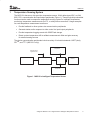
The MSC121x has an on-chip precision temperature sensor, 24-bit delta-sigma ADC, an 8-bit
8051 CPU, communication and input/output peripherals (Figure 1). These single chip-embedded
functions can be used to compose a temperature sensing system for intelligent temperature
monitoring, temperature measurements for IPC, or cold-junction-corrections. Usage examples
for such temperature measurement results are:
•
Provide feedback to other systems via communication peripherals
•
Generate status and/or response to other control via input/output peripherals
•
Provide temperature-logging record with 32KB Flash storage
•
Detect system temperature drift to calibrate measurement offset and gain accuracy
for external analog sources
The device communication peripherals include a variety of industrial standards: UART (dual),
SPITM, and I2C (MSC1211 only).
Communication
Peripherals
External Analog
Signal Sources
Temperature Sensor
24 bit Delta-Sigma ADC
8051 CPU
32KB Flash
Memory
I/O
Peripherals
Figure 1. MSC121x Intelligent Temperature Sensor
Using the MSC121x as a High-Precision Intelligent Temperature Sensor
3
SBAA100
1.1
Temperature Sensor Circuit
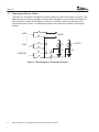
The MSC121x has a pair of temperature sensing diodes D1 and D2, as shown in Figure 2. The
differential inputs of the on-chip ADC converter are selectable via input multiplexers. When the
ADC multiplexer control (SFR ADMUX) is set to FFH, the ADC inputs are connected to the
temperature diode outputs. The differential voltage of the diode pair provides a temperature
reading.
AIN0
.
.
.
To ADC
ID1
AIN7
D1
AINCOM
Figure 2. Block Diagram of Temperature Sensor
4
Using the MSC121x as a High-Precision Intelligent Temperature Sensor
ID2=80*ID1
D2
SBAA100
1.2
Temperature Sensor Parameters
The theory of using a silicon diode to measure temperature is discussed in the TI Application
Report, Measuring Temperature with the ADS1216, ADS1217, or ADS1218 [2]. Most of the discussion from this bulletin applies to the MSC121x design. Equation 1 shows the PN junction
ideal diode equation. Table 1 shows the parameter description for the diode equation. In the
MSC121x implementation, IDIODE is from a constant current source. IS is the only temperature−
dependent parameter. To eliminate IS, differential measurement is used.
VDIODE =
I
nkT
ln( DIODE )
q
Is
Equation 1. Ideal Diode Equation
Parameters
Descriptions
VDIODE
Diode voltage
n
Diode emission coefficient (typical value = 1)
k
Boltzman constant = 1.3806503E−23 J/ °K
T
Absolution Temperature (°K)
q
Charge of an electron = 1.602176462E−19 C
IDIODE
Diode current
IS
Diode saturation current (function of diode design and temperature)
Table 1. Diode Equation Parameters
The diode voltages for D1 and D2 in Figure 2 are VD1 and VD2, respectively. The difference of
the diode voltages is Vtemp. The constant current applied to the diodes, ID1 and ID2, is designed
such that ID2 = 80*ID1. The two diodes are also designed such that diode saturation currents, IS,
of the two diodes are identical. Identical IS are achieved by closely matching the two diode feature sizes and applying silicon layout techniques to reduce process variation for components on
the same silicon die. Therefore, as shown in Equation 2, the diode pair output voltage Vtemp is
proportional to the absolute temperature T, where α is a temperature−independent constant.
Vtemp = VD1 − VD 2 =
I
I
I
nkT
nkT
[ln( D1 ) − ln( D 2 )] =
ln( D1 ) = aT
q
Is
Is
q
I D2
Equation 2. Differential Diode Equation
The MSC121x device Vtemp measurement results do not exactly match with Equation 2. Examples for the sources of deviation from Equation 2 are:
•
Diode emission coefficient, n, in Equation 1 is a function of IDIODE; therefore, the
assumption that n equals 1 should be corrected
•
Perfectly matching D1 and D2 is not possible; therefore, the saturation currents (IS)
of D1 and D2 are not identical
Using the MSC121x as a High-Precision Intelligent Temperature Sensor
5
SBAA100
1.3
•
The ratio of ID1 and ID2 is not temperature-independent; therefore, when the diode pair
differential voltage is calculated from the temperature in Equation 2, the resulting voltage
has a high-order term of T (for example, Vtemp= aT2+bT+c).
•
The ratio of ID1 and ID2 is not identical across each device; therefore, a single α value
cannot be used for all devices
•
The coefficients are calibrated to the temperature range of interest; thus, extrapolation
beyond this range will result in error. For instance, when T = 0°K, the voltage is not equal
to zero.
Ideal Diode Equation
Vtemp =
nk ln(80)
(Tc + 273.15) = mTc + c
q
Equation 3. Linear Temperature Equation
Ideal Diode
Linear Curve Fitted
Polynomial Curve Fitted
Slope Coefficient
m (µV/5C)
Intercept Coefficient
c (mV)
Curve Fitting
Accuracy (5C)
System Accuracy
(5C)
nk*ln(80)/q = 377.6
m*273.15 = 103.1
NA
NA
+0.44/−0.30
+0.045/−0.048
+0.49/−0.35
+0.095/−0.098
386.7
104.98
Vtemp = 6.3595E−5 Tc2 + 0.3842 Tc + 104.90
Table 2. Temperature Sensor Slope and Intercept Coefficients
Converting the voltage to temperature using a linear equation simplifies conversion computation.
Equation 2 is rearranged to a linear format to give Equation 3. Following are characteristics of
Equation 3:
•
°Celsius is used instead of °Kelvin (°Celsius = °Kelvin –273.15)
•
Constant current ratio between ID1 and ID2 equals 80
•
Tc is the diode temperature in °C
•
m is the temperature slope coefficient
•
c is the temperature intercept coefficient
The slope coefficient, m, and intercept, c, represent the gain and offset, respectively, of the
temperature equation. When the constants of the ideal diode equation (Table 1) are used for
Equation 3, coefficients for the ideal equation can be calculated. The values are shown in the
Ideal Diode row of Table 2. For physical devices, m and c are different from the ideal values.
6
Using the MSC121x as a High-Precision Intelligent Temperature Sensor
SBAA100
2
Temperature Sensor Accuracy
2.1
Linear Curve Fitting
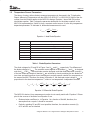
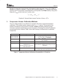
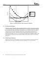
To understand if the physical device measurement result is different from that generated by the
ideal model, a linear curve fitting with least square method1 is used. Vtemp is measured for 15
temperature points2 within the range of –40 to 85°C. Vtemp results are shown on the left y-axis of
Figure 3. The measurement points have a very linear distribution. The linear curve fitted
coefficients are shown on the Linear Curve Fitted row of Table 2. The coefficients are within
2.5% of the ideal coefficients.
The linear curve fitted result also shows the precision of the temperature measurement system.
When the curve fitted coefficients are used to calculate temperature from measured Vtemp, the
error of the system is shown on the line Linear Err, referencing the right-y-axis of Figure 3. The
error of linear curve fitting is within +0.44 and –0.30°C.
System accuracy is defined as the measurement accuracy when the temperature range of
interest is measured repeatedly with the curve fitting coefficients. The system accuracy result is
listed in the last column of Table 2. The curve fitting precision is affected by the measurement
equipment setup accuracy, reference temperature sensor specifications, and system
uncertainties. The measurement equipment setup accuracy for this report is around ±0.05°C.
System accuracy using linear curve fitting is ±0.5°C. This level of accuracy outperforms many
precision temperature sensors and equipment.
Each device may have unique values of m and c. If enough measurement points of (Vtemp, Tc)
are acquired for each device, and the points are linear curve fitted, a system measurement
accuracy of ±0.5°C should be achievable. In addition to high-precision measurement, another
advantage of using linear curve fitting is low computation requirements, which need only one
multiplication and one addition.
Computing Tc from Vtemp is simply the inverse function of Equation 3:
Tc =
Vtemp
m
−
c
= m’Vtemp + c’
m
Equation 4. Linear Inverse Function of Vtemp = f(Tc)
The coefficients m′ and c′ for Equation 4 could be calculated from m and c. Another possible
method for calculating m and c is that instead of using temperature for x-axis and Vtemp for
y-axis (as in Figure 3), generating the linear curve fitting results again with x-axis as Vtemp and
y-axis as temperature.
1 Microsoft Excel functions of regression are used for this report. See Microsoft Excel user’s manual for
details of regression usage.
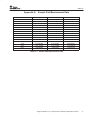
2 Measurement results table is listed in Appendix A.
Using the MSC121x as a High-Precision Intelligent Temperature Sensor
7
SBAA100
When curve-fitting results are used to compute Tc from Vtemp, this is the sensor calibration
process. This calibration process eliminates offset (c) and gain (m) error in the complete signal
chain. Example errors in the chain are interconnection offset, signal conditioning circuit
gain/offset, ADC gain/offset, reference voltage accuracy/temperature draft, and silicon
die-to-package temperature difference.
140
0.5
0.4
130
0.3
0.2
0.1
110
0.0
100
Error (deg C)
Vtemp (mV)
120
Vtemp (mV)
Linear Err (deg C)
Poly Err (deg C)
−0.1
−0.2
90
−0.3
80
−0.4
−44 −40 −30 −20
−9
1
11
21
31
41
51
60
71
80
85
Temperature (deg C)
Figure 3. MSC Vtemp (left y-axis) and Measurement Accuracy (right y-axis)
2.2
Polynomial Curve Fitting
The linear ideal equation, Equation 3, includes only a first-order effect from Tc. Vtemp is actually a
function of a higher-order effect of Tc. When the higher-order component of Tc is considered, a
new level of temperature measurement accuracy can be achieved. The Vtemp data points
(Figure 3) are curve fitted with a second-order polynomial. The Polynomial Curve Fitted row of
Table 2 shows the second-order polynomial and its coefficients. The error of temperature
measurement that occurs when this polynomial is used appears on the Poly Err curve in
Figure 3. The curve fitting error is reduced to +0.045/−0.048°C (an error range of 0.093°C),
showing improvement over the linear curve fitting method by a factor of five. When
measurement system error is considered, overall system accuracy of ±0.1°C can be achieved.
Inspecting the coefficient of the Tc2 term in Table 2, this value is much smaller than the other two
coefficients of the same equation. When third- or higher-order polynomial curve fittings for the 15
measurement points are used (see Appendix A), no significant curve fitting error reduction can
be obtained. It can be seen that third-order polynomial curve fittings may slightly reduce
measurement error. However, using a third-order polynomial increases computational
requirements.
8
Using the MSC121x as a High-Precision Intelligent Temperature Sensor
SBAA100
Equation 5 shows the inverse function of the second−order polynomial Vtemp = f(Tc) (Table 2).
Equation 5 is useful to calculate Tc from the ADC-acquired voltage Vtemp. Similar to the inverse
function of the linear equation, the coefficients for this equation can be generated by using curve
fitting with Vtemp at the x-axis and Tc at the y-axis.
2
+ b’Vtemp + c’
Tc = a ’Vtemp
Equation 5. Second-Order Inverse Function of Vtemp = f(Tc)
3
Temperature Sensor Calibration Methods
The curve fitting method is very effective for computing the linear or polynomial equation
coefficients. This method requires measuring the (Vtemp, Tc) points. The precision of the
equation increases as more points are included. However, increasing measuring points
increases equipment-manufacturing cost and complexity. Reducing the number of calibration
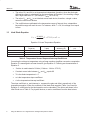
measurement points is desired. Table 3 shows the summary of different level of calibration
complexities.
Cal. Methods
Error Magnitude (5C)
Description
Zero Point
(Non-calibrated)
6.5
Use averaged slope and intercept coefficient
m′ave= 1/mave = 2582.173°C/V
c′ave = −cave/mave = −269.386°C
1 Point
2
Significant accuracy improvement with only one
point calibration
2 Points
+0.62/−0.20, Worst case ±1
Equation 3, 2 points at –10/+50°C
3 Points
Linear equ: +0.28/−0.54,
worst case ±0.7
Second−order equ: +0.07/−0.14,
worst case ±0.2°C
3 points at –40/+20/+85° C
Second-order equ matching the accuracy as 15 pts
calibrations
6 – 15 Points
±0.1
6 points with third-order polynomial
15 points with second-order polynomial
Table 3. Temperature Sensor Calibration Complexities vs. Precision
Using the MSC121x as a High-Precision Intelligent Temperature Sensor
9
SBAA100
1.5
Error (deg C)
1.0
Lin Err 1pt
Lin Error 2pt
0.5
Lin Error 3pt
Poly Error 3pt
−50
−30
0.0
−10
10
30
50
70
90
−0.5
Temperature (deg C)
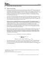
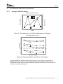
Figure 4. Increasing Accuracy with Calibration Complexity
3.1
Two Points Calibration
The linear equation, Equation 3, has two unknown coefficients, m and c. Two points are needed
to solve for m and c. When solving the equation, an error in m will introduce gain error. An error
in c will cause offset error. The Linear Err curve (Figure 3) is a parabola with the most negative
error at the bottom of the curve and the most positive errors on the top two ends of the curve.
The error at –10°C and +50°C have the minimum error. Using these two temperatures to
calibrate the linear equation gives the lowest error. These calibration point selections give a
measurement accuracy of +0.6/−0.2°C that is similar to multiple points’ calibration (Table 3). The
worst-case error would be lower than the peak-to-peak of the Figure 3 Linear Err curve that is
less than 1°C.
3.2
Three Points Calibration
The worst-case error for second-order polynomial curve fitting would be lower than half of the
peak-to-peak of the Figure 3 Linear Err curve that is less than 0.5°C, for most devices.
10
Using the MSC121x as a High-Precision Intelligent Temperature Sensor
SBAA100
Average Coefficient Values
Slope & Intercept for 6 parts
−268
2610
c’
m’
2605
−270
2600
−271
2595
−272
2590
−273
2585
−274
Slope (deg C/V)
−269
Intercept (deg C)
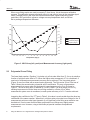
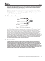
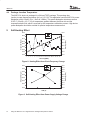
3.3.1
No Calibration and One Point Calibration
2580
1
2
3
4
5
6
Part#
Figure 5. Slope and Intercept Coefficient Histograms for 6 Samples
Error Temp (with ave m’ & c’)
5
4
3
Error (deg C)
3.3
2
1
0
−60
−40
−20
0
20
40
60
80
100
−1
−2
−3
Temperature (deg C)
Figure 6. Temperature Measurement Error for 6 Samples
In some applications, absolute measurement accuracy is not critical, so measuring the
calibration point is eliminated. For those applications that concentrate only on relative
temperature change, using the typical coefficient set would be sufficient. However, absolute
accuracy is impaired dramatically.
Using the MSC121x as a High-Precision Intelligent Temperature Sensor
11
SBAA100
Slope and intercept coefficients of actual devices were acquired for six MSC1210 samples
between the temperature of −40 and 85°C at 1MHz CPU clock frequency (clock frequency
effects will be discussed later). Figure 5 and Figure 6 show the Slope and Intercept chart and
the Temperature Error for these six sample parts. The average slope (m′ave) and intercept
coefficient (c′ave) of the samples are 2582.173°C/V and −269.386°C, respectively. The Slope
and Intercept chart shows the wide variations (5°C: from –273.5 to –269.5°C) of intercept
coefficient among all six devices. Each line of the Temperature Error chart shows the
measurement error of a sample part. The chart shows that the error value for each part
fluctuates below 2°C. These also indicate that the slope variation over the sample devices is low.
If the averaged slope/intercept coefficients are used, temperature measurement error is up to
6.5°C. This error can easily reduce down to 2°C if the intercept coefficient variation is calibrated.
3.3.2
One Point Calibration
One point calibration for a linear equation with two unknown factors requires either the averaged
slope or averaged intercept coefficient. As shown in Figure 5, calibrating the intercept coefficient
corrects most of the error. When one point calibration is used with the averaged slope coefficient
to calculate the intercept coefficient, the error is reduced by more than 4.5°C and reach below
2°C (Figure 4).
3.3.3
Measurement Setups
To minimize self-heating errors, the measurements use a 1MHz clock frequency and 3V power
supply.
The curves shown in Figure 5 were acquired when an internal reference voltage is used.
Because the temperature stability of the internal reference voltage is trimmed during the device
manufacturing process, the slope (gain) coefficient is very stable. The internal reference voltage
was able to achieve all the temperature measurement accuracy described in Table 3.
4
Calibration Setups
4.1
Reference Sensor
This report uses an RTD temperature sensor to calibrate the MSC121x measurements. YSI
Precision Temperature Group manufactures the RTD sensor, model 55031 [3]. The
measurement accuracy is trimmed to within 0.05°C. The RTD resistance to temperature
relationship is shown in Equation 6.
T = (a + b ln( R ) + c ln( R ) 3 ) −1
Equation 6. RTD Resistance to Temperature
12
Using the MSC121x as a High-Precision Intelligent Temperature Sensor
SBAA100
R is in ohms, a/b/c are constants, and T is in °Kelvin. Equation 6 coefficients are measurement
temperature range dependent. A different set of a, b, and c are used for a specified range of
temperature. Once the sensing temperature range is defined, these factors are constant. YSI
provided an Excel file to calculate the coefficients.
∂R/∂T (Ω per °C) defines the requirement of measurement accuracy. For example, at 25°C,
∂R/∂T = −99 Ω/°C, R is around 2.2kΩ. To measure 0.05°C, a DMM needs to have resolution of
5−Ω (99*0.05) for the range setting for 2kΩ. The ∂R/∂T values for different temperatures are
supplied with the YSI attached Excel file.
4.2
Reference Sensor Measurements
Source+
RTD
Sense+
Sense−
Source−
HV Shield
Figure 7. RTD 5 Wires Configuration
An HP3458A Digital Multimeter is used in this report to measure the RTD resistance. Figure 7
shows the 5 wires connection used for RTD resistance measurement the meter supports.
(Sense+, Sense−) connection pair is for RTD voltage sensing inputs. This pair carries almost
zero current to avoid measuring any voltage drop caused by lead connections resistance.
(Source+, Source−) connection pair is for excitation current for resistance measurement. The
current from the meter is less than 100µA to minimize the RTD self-heating effect caused by I−R
drop. This meter is able to measure better than 0.05°C over the RTD resistance range within its
corresponding temperature. The HV Shield connection (Figure 7) protects the measurement
from noise interference and external high voltage discharge.
4.3
Temperature Bath
A stable temperature bath helps to reduce both the self-heating effect and the temperature
gradient caused by the device package, and provides a constant temperature for calibration.
The self-heating effect will be discussed in Section 5. H-Galden ZT 180 [4], a heat transfer fluid,
is used in the bath. It is a non-electric-conducting, thermally- and chemically-stable fluid. To
increase the effectiveness of the bath, a 1A stirring fan with a PWM speed control circuit is used
to break the H-Galden fluid ventilation, and to maintain constant temperature over the bath. The
temperature bath is placed inside a programmable oven to perform calibration.
Using the MSC121x as a High-Precision Intelligent Temperature Sensor
13
SBAA100
4.4
Package Junction Temperature
The MSC121x device is packaged in a 64-lead TQFP package. This package has
junction-to-case thermal resistance (θJC) of 4.3°C/W. This application controls MSC121x power
dissipation within 3.6mW (3V x 1.2mA at 1.8MHz). This power dissipation introduces a mere
0.015°C (3.6mW x 4.3°C / W) of temperature gradient between the silicon die and the
temperature bath fluid, which is removed by the temperature calibration process. High device
power dissipation should be avoided for precise temperature measurement.
Self-Heating Effect
382.5
108.0
m
382.0
c
107.5
Slope (uV/deg. C)
381.5
107.0
381.0
106.5
380.5
106.0
380.0
105.5
379.5
Intercept (mV)
5
105.0
379.0
378.5
104.5
1
3
5
7
9 11 13 15 17 19 21 23 25 27 29 31 33
Clk Freq (MHz)
Figure 8. Heating Effect from Clock Frequency Change
376.4
106.0
m
105.9
c
376.2
105.7
105.6
375.8
105.5
375.6
105.4
105.3
375.4
Intercept (mV)
Slope (uV/deg. C)
105.8
376.0
105.2
375.2
105.1
375.0
105.0
3
4
VDD (V)
5
Figure 9. Self-Heating Effect from Power Supply Voltage Change
14
Using the MSC121x as a High-Precision Intelligent Temperature Sensor
SBAA100
Heat generated by sensors when power is applied causes self-heating. When the MSC121x
operates as a temperature sensor, the applying power introduces self-heating and affects the
calibration coefficient. The device heat dissipation is proportional to the power supply voltage,
operation frequency, and on-chip operating features. Figure 8 and Figure 9 show the
self-heating effect on slope and intercept coefficients when the device operation frequency or
supply voltage is increased. If the coefficients are calibrated, the self-heating effect is removed
with the calibration process. However, if the coefficients are not calibrated, or the application
environment is very different from the environment when the coefficients are prepared, minimum
heat dissipation from the device is preferred. Minimum heat dissipation requires a lower power
supply voltage and clock frequency. The lowest heat dissipation condition recommended for the
MSC121x is 1 MHz clock frequency with 3V power supply.
6
Example Code
The MSC1210-DAQ-EVM [5] board is used for running the example code. Raisonance IDE is
used for the code development. The clock frequency is running at 1.8432MHz. The power
supply is at 3V. Appendix B lists the source code, using floating-point math. The size of the code
is 3kB, which is supported by the Raisonance 4kB Demo Version.
To minimize power consumption, unused peripherals are shut off. The PSEN and ALE pins are
also turned off.
PDCON &= 0x0f7;
PASEL=0xff;
//turn on adc
List 1 . Power Control
ADC is set to convert at 7SPS. Since the DAQ-EVM used is calibrated, temperature drift error is
canceled by the calibration. Instead of using an external reference voltage, the internal reference
is used.
ACLK=1;
DECIMATION = 0x7ff;
ADCON0 = 0x20;
ADMUX=0xff;
ADCON1 = 0x01;
// ACLK = 1.8432MHz/(1+1)= 0.9216MHz
// Vref on 1.25V, Buff off, BOD off, PGA 1
// bipolar, auto, self calibration, offset, gain
List 2 . ADC Setup
The on-chip summation register is used. The 7 SPS conversion is further averaged by 32 times.
SSCON=0;
SSCON=0xe4;
// Clear SUMR0~3
// Set SSCON for ADC 32 summations and div by 32
List 3 . On-chip summation register setup
In order to achieve resolution higher than 0.01°C, a moving-window of size 32 is used. The
linear and polynomial equations are calculated with 32-bit floating point math.
Using the MSC121x as a High-Precision Intelligent Temperature Sensor
15
SBAA100
tc_lin=M0*vt + C0;
tc_poly=A1*vt*vt + B1*vt +C1;
List 4 . 32-bit floating point math library calculates the linear and polynomial equations
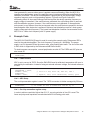
To minimize code memory usage, a recursive routine print is added instead of the library printf.
printf with a floating point requires over 1kB additional memory, while print and its calling routine
need only 234 bytes.
References
[1] MSC1210/MSC1211/MSC1212 Product Data Sheets (SBAS203A, SBAS267, SBAS278)
[2] Measuring Temperature with the ADS1210, ADS1217, or ADS1218 (SBAA073)
[3] YSI Precision Temperature Group http://ww.ysi.com
[4] Solvay Solexis: http://www.solvaysolexis.com/pdf/h_gald_zt180.pdf
[5] MSC1210-DAQ-EVM User’s Guide and Examples (SBAU083)
16
Using the MSC121x as a High-Precision Intelligent Temperature Sensor
SBAA100
Appendix A.
Sample Part Measurement Data
Temperature (5C)
−44.36
Vtemp (mV)
87.92666435
Linear Error
0.438626575
Poly Error
0.044972785
−39.6
−30.07
89.71338287
93.35722938
0.251329446
0.121571235
−0.047687135
−0.006194279
−19.54
−9.34
97.39257813
101.3098907
−0.019675812
−0.142078513
0.008144526
0.002530738
0.67
11.18
105.1522636
109.215641
−0.249363725
−0.269842725
−0.022975509
0.00771484
21.39
31.01
113.1717587
116.8513966
−0.263136332
−0.300837209
0.029364017
−0.025324675
40.77
50.58
120.6834221
124.5174599
−0.191998502
−0.158498335
0.034180009
−0.013989796
60.31
70.94
128.3015156
132.4857807
−0.063606864
0.155197957
−0.031392908
0.026589074
80.18
85.01
136.1010933
138.0062601
0.297174865
0.39513794
−0.001386513
−0.004545181
Table A−1. Sample Part Measurement Data
Using the MSC121x as a High-Precision Intelligent Temperature Sensor
17
STDZ001A
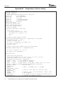
Appendix B.
Temperature.c Source Listing
#include <REG1210.H>
#include <stdlib.h>
#include <math.h>
// Vref=1.25V, bipolar results give 1.25*2/2^24
#define LSB
(1.25/8388608)
#define M0
2586.67098545498
#define C0
−271.7529
#define A1
−1.08436244851484e3
#define B1
2.83158996601634e3
#define C1
−285.1293
#define WINDOWSIZE
16
signed long summer(void);
extern void putspace4(void);
extern void tx_byte(char);
// Print a message
void putstr(char code * data msg)
{
while (*msg != 0) {
tx_byte((unsigned char) *msg);
if( *msg==’\n’) tx_byte(’\r’);
msg++;
}
}
// recursive digit display routine
void prt_digit(unsigned long int i, signed char d) reentrant
{ unsigned long int j; char c;
j=i/10; c=i−j*10; d−−;
if (j!=0 || !(d &0x80)) prt_digit(j,d);
if (d==0) tx_byte(’.’);
tx_byte(c+48);
}
// Display long integer number with sign and decimal
void print(signed long int i, unsigned char d)
{
if (i<0) { tx_byte(’−’); i*=−1;}
prt_digit(i,d); putspace4();
}
void main(void)
{
signed long int data sum;
float data window[16]={0,0,0,0, 0,0,0,0, 0,0,0,0, 0,0,0,0};
float data adres=0, vt, tc_lin, tc_poly;
unsigned char fill_ptr=1, mod_ptr=0;
T2CON = 0x34;
// T2 as baudrate generator
RCAP2 = 65535; // 57600 Baud @ 1.8432MHz
SCON
= 0x52;
// Async mode 1, 8−bit UART, enable rcvr, TI=1, RI=0
putstr(”\x1b[1;33;46m\x1b[2J\x1b[12CTemperature Sensor\n”);
PDCON &= 0x0f7;
//turn on adc
PASEL=0xff;
ACLK=1;
// ACLK = 1.8432MHz/(1+1)= 0.9216MHz
DECIMATION = 0x7ff;
ADCON0 = 0x20;
// Vref on 1.25V, Buff off, BOD off, PGA 1
ADMUX=0xff;
ADCON1 = 0x01;
// bipolar, auto, self calibration, offset, gain
SSCON=0;
// Clear SUMR0~3
SSCON=0xe4;
// Set SSCON for ADC 32 summations and div by 32
sum=summer();
// Discard 1st summation result
18
Using the MSC121x as a High-Precision Intelligent Temperature Sensor
STDZ001A
SSCON=0;
// Clear SUMR0~3
SSCON=0xe4;
// Set SSCON for ADC 32 summations and div by 32
while(1){
sum=summer();
SSCON=0;
// Clear SUMR0~3
SSCON=0xe4;
// Set SSCON for ADC 32 summations and div by 32
adres=adres−window[mod_ptr];
// Moving Window of 10 results
window[mod_ptr]=(float) sum;
adres=adres+ window[mod_ptr];
vt=adres/(float)fill_ptr*LSB;
tc_lin=M0*vt + C0;
print((signed long int)(tc_lin*1000),3);
tc_poly=A1*vt*vt + B1*vt +C1;
print((signed long int)(tc_poly*1000),3);
if (fill_ptr==WINDOWSIZE) fill_ptr=WINDOWSIZE; else fill_ptr++;
if (mod_ptr==(WINDOWSIZE−1)) mod_ptr=0; else mod_ptr++;
putstr(”\n”);
if (RI==1){ // Any key will pause, any key again to start
putstr(”Pause....”);
RI=0;
while(RI==0) {;}
putstr(”Continue\n”);
RI=0;
}
}
}
Using the MSC121x as a High-Precision Intelligent Temperature Sensor
19
IMPORTANT NOTICE
Texas Instruments Incorporated and its subsidiaries (TI) reserve the right to make corrections, modifications,
enhancements, improvements, and other changes to its products and services at any time and to discontinue
any product or service without notice. Customers should obtain the latest relevant information before placing
orders and should verify that such information is current and complete. All products are sold subject to TI’s terms
and conditions of sale supplied at the time of order acknowledgment.
TI warrants performance of its hardware products to the specifications applicable at the time of sale in
accordance with TI’s standard warranty. Testing and other quality control techniques are used to the extent TI
deems necessary to support this warranty. Except where mandated by government requirements, testing of all
parameters of each product is not necessarily performed.
TI assumes no liability for applications assistance or customer product design. Customers are responsible for
their products and applications using TI components. To minimize the risks associated with customer products
and applications, customers should provide adequate design and operating safeguards.
TI does not warrant or represent that any license, either express or implied, is granted under any TI patent right,
copyright, mask work right, or other TI intellectual property right relating to any combination, machine, or process
in which TI products or services are used. Information published by TI regarding third-party products or services
does not constitute a license from TI to use such products or services or a warranty or endorsement thereof.
Use of such information may require a license from a third party under the patents or other intellectual property
of the third party, or a license from TI under the patents or other intellectual property of TI.
Reproduction of information in TI data books or data sheets is permissible only if reproduction is without
alteration and is accompanied by all associated warranties, conditions, limitations, and notices. Reproduction
of this information with alteration is an unfair and deceptive business practice. TI is not responsible or liable for
such altered documentation.
Resale of TI products or services with statements different from or beyond the parameters stated by TI for that
product or service voids all express and any implied warranties for the associated TI product or service and
is an unfair and deceptive business practice. TI is not responsible or liable for any such statements.
Following are URLs where you can obtain information on other Texas Instruments products and application
solutions:
Products
Applications
Amplifiers
amplifier.ti.com
Audio
www.ti.com/audio
Data Converters
dataconverter.ti.com
Automotive
www.ti.com/automotive
DSP
dsp.ti.com
Broadband
www.ti.com/broadband
Interface
interface.ti.com
Digital Control
www.ti.com/digitalcontrol
Logic
logic.ti.com
Military
www.ti.com/military
Power Mgmt
power.ti.com
Optical Networking
www.ti.com/opticalnetwork
Microcontrollers
microcontroller.ti.com
Security
www.ti.com/security
Telephony
www.ti.com/telephony
Video & Imaging
www.ti.com/video
Wireless
www.ti.com/wireless
Mailing Address:
Texas Instruments
Post Office Box 655303 Dallas, Texas 75265
Copyright  2004, Texas Instruments Incorporated