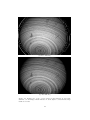
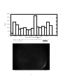
1
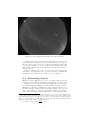
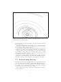
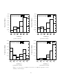
Detecting clouds in a starlit sky
University of Cambridge Part III Physics Project
∗
Ben Webb
Supervisor: Dr D F Buscher
June 27, 2013
Abstract
I describe a method for automatically determining cloud cover statistics for images taken by an all-sky CCD camera at the Magdalena Ridge
Observatory. Unlike previous techniques, this method does not rely on
properties of the lens or existing star catalogues.
Instead, the same star was identified across multiple images, by tracking its movement in small steps across composite images. These composite
images were produced by combining images taken at similar sidereal times.
The visibility an image was calculated as the ratio of the flux of all
stars to the expected flux of all stars. Errors of the order of 10% were
found in this calculated visibility.
Various sources of error are discussed. The appearance of the moon
in images was found to have an adverse effect on the accuracy of the
computed visibility.
Statistics were aggregated by night. 24% of nights were found to be
entirely clear of cloud, whereas 9% were entirely cloudy.
The method used is expected to be applicable for images from other
similar cameras.
∗ This
report is, for the most part, the same as the one submitted at the end of the project.
Some small alterations have been made for correctness. The source code of the project can
be found online: https://github.com/Bjwebb/detecting-clouds
1
Contents
1 Introduction
3
2 Method
2.1 Images used . . . . . . . . .
2.1.1 Moonlit images . . .
2.2 Initial image filtering . . . .
2.3 Sidereal time grouping . . .
2.4 Extracting objects . . . . .
2.5 Extracted object filtering .
2.6 Matching extracted objects
2.7 Post-matching filtering . . .
2.8 Calculating image visibility
.
.
.
.
.
.
.
.
.
.
.
.
.
.
.
.
.
.
.
.
.
.
.
.
.
.
.
.
.
.
.
.
.
.
.
.
.
.
.
.
.
.
.
.
.
.
.
.
.
.
.
.
.
.
.
.
.
.
.
.
.
.
.
.
.
.
.
.
.
.
.
.
.
.
.
.
.
.
.
.
.
.
.
.
.
.
.
.
.
.
.
.
.
.
.
.
.
.
.
.
.
.
.
.
.
.
.
.
4
5
5
5
5
6
7
7
8
9
3 Results
3.1 Matching of stars across multiple images
3.2 Visibility values . . . . . . . . . . . . . .
3.3 Classifying visibility . . . . . . . . . . .
3.4 Statistics by night . . . . . . . . . . . .
.
.
.
.
.
.
.
.
.
.
.
.
.
.
.
.
.
.
.
.
.
.
.
.
.
.
.
.
.
.
.
.
.
.
.
.
.
.
.
.
.
.
.
.
10
10
10
13
17
4 Discussion
4.1 Sources of error . . . . . . . . . . . . . . . . . . . .
4.1.1 Assumptions when calculating the visibility
4.1.2 Inclusion of moonlit images . . . . . . . . .
4.1.3 Measuring cloud cover by eye . . . . . . . .
4.1.4 Falsely identifying objects . . . . . . . . . .
4.1.5 Moonlit cloud . . . . . . . . . . . . . . . . .
4.1.6 Error in identifying stars . . . . . . . . . .
4.1.7 Errors in matching . . . . . . . . . . . . . .
4.1.8 Variation in flux of individual stars . . . . .
4.1.9 Camera operation bias . . . . . . . . . . . .
4.2 Potential further work . . . . . . . . . . . . . . . .
.
.
.
.
.
.
.
.
.
.
.
.
.
.
.
.
.
.
.
.
.
.
.
.
.
.
.
.
.
.
.
.
.
.
.
.
.
.
.
.
.
.
.
.
.
.
.
.
.
.
.
.
.
.
.
19
19
19
19
20
20
20
22
24
24
24
27
.
.
.
.
.
.
.
.
.
.
.
.
.
.
.
.
.
.
.
.
.
.
.
.
.
.
.
.
.
.
.
.
.
.
.
.
.
.
.
.
.
.
.
.
.
.
.
.
.
.
.
.
.
.
5 Conclusion
28
6 References
29
A Visualising the Data
30
A.1 Generating PNG images from FITS files . . . . . . . . . . . 30
A.2 Data explorer interface . . . . . . . . . . . . . . . . . . . . . 30
B List of Figures
31
2
Chapter 1
Introduction
The Magdalena Ridge Observatory (MRO) is a recent telescope site,
home to a 2.4 meter fast tracking optical telescope. A ten-element optical/infrared interferometer is also under construction at the same site.
Optical telescopes require clear sky to function well.
In order to measure cloud cover, an all-sky camera was installed at
the site. A 2004 analysis of images from this camera found that 23% of
nights were completely clear of clouds.[1] This number was obtained by
measuring the cloud cover for each night by eye. This becomes tedious as
the number of images increases.
In this report I present a method of automatically determining the
cloud cover. I apply it to images taken by same camera during 2012 and
2013.
Such automatic measurements have been made for other all sky cameras. This has been achieved by using information about projection of
the lens to compare the stars in images to those in existing star catalogues.[2][3]
In contrast, my method does not rely on such properties of the camera
setup, or require the use of existing star catalogues. Instead, dimming of
stars is identified by comparing each stars across multiple images.
3
Chapter 2
Method
§2.1
Remove
Short
Lines
Select
Images
§2.7
§2.2
Filter
Saturated
Pixels
§2.3
Group by
Sidereal
Time
SExtractor
Filter
Extracted
Objects
Match
Points to
Sidereal
Points
SExtractor
Filter
Extracted
Objects
Connect
Average
Points
§2.4
§2.5
§2.6
Remove
Outlying
Fluxes
Calculate
Image
Visibility
Figure 2.1: Overview of the method used
Cloud cover was estimated by comparing the flux of stars in an image
to the flux of the same stars in other images (section 2.8).
This requires identifying the stars in an image (section 2.4), and then
matching the same star across multiple images. Since the images do not
offer a continuous view of a star (for example, due to cloud cover and
daytime) it is not easy to track a star across them.
Instead, composite images were produced for a series of sidereal time
ranges (section 2.3). These were used to follow the positions of stars.
The same star in multiple individual images was then identified using the
information from the composite images. (section 2.6)
Various filtering steps (sections 2.2, 2.5 and 2.7) were applied to ensure
that only real stars were used.
4
§2.8
2.1
Images used
Images taken by the all sky camera between 25th March 2011 and 30th
November 2012 were used.1 During this time period, images were recorded
with a 15 second exposure, every 5 minutes, when possible (subsection 4.1.9
discusses this in more detail). Earlier images for 2011 were available, but
were unsuitable due to differing exposure times and image resolutions.
2.1.1
Moonlit images
Images containing the moon present several challenges. The brightness of
the moon obscures stars, leading to a lower calculated visibility than for
the same conditions without the moon. For these reasons, I calculated results for both the cases when moonlit images were included and excluded.
The real amounts of cloud cover are expected to the same[4].
In order to calculate results for only non-moonlit images, it was first
necessary to determine which images were moonlit. The moon leads to
many more high valued pixels than all of the stars combined. As a result,
the sum of an image’s pixels is greater the more moonlight is visible.
However, since the moon can illuminate the sky when it is just out of
sight, the amount of moonlight an image can have is continuous. In order
to definitely include all images that contain the moon, I define images to
be moonlit if:
X
pixels in an image ≥ 2 × 10⁸
2.2
Initial image filtering
Saturated pixels were removed by replacing any values greater than a fixed
threshold with 0. Some pixels lit by the moon also exceed this value, but
only if they are lit directly. Since such pixels would otherwise contain the
image of the moon, there is no adverse effect on my calculation of cloud
cover.
2.3
Sidereal time grouping
The following definition of sidereal time was used:
ts = ∆t
Where
ts
∆t
L
=
=
=
=
mod L
Sidereal time (seconds)
Seconds since 2011-01-01 00:00:00
Length of mean sidereal day
86164.091 seconds [5]
There is a fixed offset to other definitions of sidereal time. This does
not matter, since I will not compare my sidereal times to any from other
sources.
Images were binned (ie. grouped) into minute long ranges of sidereal
time. This left 4 seconds unaccounted for. The two images with a sidereal
time in this range were discarded. Any bias to my calculations due to
losing these two images is much smaller than that due to other errors.
1 All
dates and times given in UTC
5
Figure 2.2: An example sidereal time bin composite image
Stars should be in the same positions when the sidereal time is the
same.2 Thus, in each bin, the positions of stars will vary by 0.25 degrees.3
Since the images show 180 degrees of sky in less than 640 pixels, this
corresponds to a variation of no more than 0.9 pixels. Thus in each of the
images in the bin, the same stars will always be in the same position or
adjacent positions.
Images containing the moon (see section 2.1) were removed from these
bins. Then, composite images were created for each bin by summing the
pixel values from each image. (See Figure 2.2 for an example.)
2.4
Extracting objects
SExtractor (Source Extractor) is a piece of software that detects and
measures sources in astronomical images. [7] In this project, it was used
to extract the positions of stars from the individual and composite images.
For individual images, SExtractor’s flux estimation was also obtained.
This flux is computed by summing the values of all pixels in an object,
and subtracting the estimated sum of pixel values if that object were not
there. As a result it does not have well defined units, but comparisons
of the flux between images will be valid if they are taken using the same
2 A mean sidereal day is actually defined as the time for one rotation of the Earth relative
to the vernal equinox. Since this precesses, a mean sidereal day is actually 0.0084 seconds
shorter than the actual period of the rotation relative to the fixed stars. [6] This amounts to
just over 5 seconds difference from my first image to my last image. Since this is much smaller
than my bin size, it will not have an important effect.
3 360 ÷ number of bins = 360 ÷ ( 86160 ) = 0.25
60
6
Figure 2.3: The mask applied to objects after extraction. The black area indicates objects that were included. It consists of two semicircles, fitted by eye to
cover as much sky as possible whilst only including sky.
setup.
In order to extract the maximum number of valid stars, several of the
default SExtractor configuration parameters were changed.
Minimum Detection Area Set to 1 pixel, since some stars in the images only fill 1 pixel
Background Mesh Size Reduced considerably, since the background of
these images is much more variable (due to the possibility of cloud
cover, and the edge of the sky) than the clean images of star fields
SExtractor is often used for.
Minimum Contrast for Deblending Deblending refers to treating flux
maxima separated by a non-background minimum as separate objects. The minimum contrast controls how deep this minimum must
be for deblending to occur. The stars in these images are sufficiently
small that double peaks will not occur for one object, so deblending
is always optimal. Thus, the minimum contrast was set to 0.
2.5
Extracted object filtering
SExtractor extracts several types of objects that are not stars. These
include objects outside of the sky, clouds illuminated by the moon, and
planets.
In this set of images, none of the stars are greater than 20 pixels wide
or high. Therefore all such objects are ignored.
A simple mask was created (Figure 2.3), that covers only those parts of
the image where the sky is visible. Objects outside this mask are ignored.
Unfortunately, some small areas of sky near the horizon are not contained
in the mask, due to the difficultly of including these areas whilst excluding
non-sky areas.
2.6
Matching extracted objects
Two objects in different composite images are identified as being the same
star if they have similar positions, and the composite images are for similar sidereal times. This equivalence is transitive. I limited matching to
objects within a 3 pixel distance of each other, and where the sidereal
time difference is no greater than 4 minutes. Objects are matched across
7
Figure 2.4: Lines drawn for the tracks of a random selection of the objects
extracted from a composite image
several bins in case the star is missing from the adjacent bin (discussed in
subsection 4.1.6).
Sometimes multiple matches were found for an object. In this case, the
objects with the smallest sidereal time difference were chosen. Of those,
the object at the shortest distance was used.
By this method, the line a star takes is slowly tracked across the sky.
A graphical representation of several such tracks can be seen in Figure 2.4.
Objects extracted from individual images were then matched against
those from the corresponding composite image. Those pairs of objects
with positions closer than 3 pixels were considered to match. In the case
of conflicts, the nearest objects were chosen.
It can now be inferred which objects match between different individual images (ie. those which are the same star), as they will have both been
matched to composite objects which have been matched to each other.
2.7
Post-matching filtering
Any suspected stars where less than 200 objects were matched in the
composite images were discounted. A typical star will appear in 600 or
more composite images. Objects appearing in less than 200 are likely to
not be stars, or to be stars that are not extracted or matched consistently
(see subsection 4.1.7 for more discussion of this).
Objects with negative fluxes, or fluxes anomalously high for their line
were also discarded.
8
Negative fluxes arise when the flux of an object is smaller than that
of the surrounding background. These occur due to patches of sky surrounded by illuminated cloud. Such objects may be safely discarded.
Some objects that are not stars are falsely matched to lines. These
objects can have wildly different fluxes, which will skew the calculated
visibility. Visual inspection shows that the flux of almost all valid stars
does not exceed three times their median flux. Therefore, all points lying
outside this range were discarded.
2.8
Calculating image visibility
With ideal data, the absolute visibility of an image could be defined:
P
Flux
stars in image
P
Visibility =
Maximum flux
stars expected
The expected stars for an image are those in the corresponding composite
image. The maximum flux is calculated across all images.
However, the real maximum flux of a star is difficult to determine,
since other objects with greater flux are misidentified as it.
Assuming all stars have the same flux distribution, replacing the median gives a scaled version of the real visibility. This allows us to calculate
the relative visibility:
P
Flux
stars in image
P
Visibility =
Median flux
stars expected
The median flux is calculated across all images.
Whereas the absolute visibility has a maximum value of 1, the relative
visibility could take arbitrarily high values. In practice however, stars
are detected more often when they are close to their maximum flux, so
the median is close to the real maximum value. As a result, the relative
visibility for clear images is close to 1. No images were found with a
relative visibility any greater than 1.2.
Throughout the rest of this report I will refer to this calculated relative
visibility simply as the visibility.
9
Chapter 3
Results
3.1 Matching of stars across multiple images
SExtractor successfully extracts the supermajority of stars visible in images.
Using the method described above, 3667 distinct stars were found.
These corresponds to 53% percent of objects extracted by SExtractor
(which do not fail the most basic tests of not being a star, such as being
outside the sky or being overly large). On average, there were 503 correctly
matched stars in each image. Inspecting a sample of such objects by eye
shows that the majority are matched correctly.
The most common problem is for a single star to have been falsely
identified as being two or more distinct stars (ie. the tracking of that
star’s progress across the sky in the composite images has been broken,
note the broken lines in Figure 2.4).
There were also a small number of ‘stars’ where two different stars were
being tracked. These problems are discussed further in subsection 4.1.7.
3.2
Visibility values
My computed visibility values (Figure 3.1 for a sample month) were seen
to be a reasonable indicator of cloud cover, when compared by eye to the
cloud cover at each point.
For nights where the amount of cloud cover varies (e.g. Figure 3.2b),
the change in cloud cover in the images is strongly related to the change in
the computed visibility. This can be seen clearly on an animation through
the images that tracks the position on the flux graph. 1
Nights that are entirely clear are expected to have a constant visibility,
since all images are entirely free of cloud. However, there is variation in
my computed visibility values. The amount of variation is similar for all
such nights. By inspecting the magnitude of the variation for a typical
clear night (Figure 3.2a), an error estimate for of 0.1 was obtained for the
high visibility limit.
1 A custom interface was built to allow such animations to be quickly viewed for any
visibility or flux plot. See section A.2 for more details.
10
1.2
1
Visibility
0.8
0.6
0.4
0.2
0
02
04
06
08
10
12
14
16
18
20
22
24
26
28
30
01
22
24
26
28
30
01
Time (Day of month)
(a) All Images
1.2
1
Visibility
0.8
0.6
0.4
0.2
0
02
04
06
08
10
12
14
16
18
20
Time (Day of month)
(b) Non-moonlit images only
Figure 3.1: Computed visibility for images taken during March 2012
11
1.08
1
1.06
0.9
1.04
0.8
0.7
Visibility
Visibility
1.02
1
0.98
0.96
0.6
0.5
0.4
0.3
0.94
0.2
0.92
0.1
0.9
0
02
04
06
08
10
12
02
04
Time (Hours)
06
08
10
12
Time (Hours)
(a) Example clear night (24th March 2012)
(b) Example variable night (26th March 2012)
0.007
0.2
0.18
0.006
0.16
0.14
Visibility
Visibility
0.005
0.004
0.003
0.12
0.1
0.08
0.06
0.002
0.04
0.001
0.02
0
0
02
04
06
08
10
12
02
Time (Hours)
(c) Example cloudy night without moon (20th March 2012).
No stars are visible for any of the images in this night.
04
06
08
10
Time (Hours)
(d) Example cloudy night with moon (9th March 2012).
For all images after 05:00, no stars are visible.
Figure 3.2: Computed visibility for selected nights during March 2012.
12
12
Cloudy
Visiblity (v) Range
0.0 ≤ v < 0.03
0.03 ≤ v < 0.15
0.15 ≤ v < 0.3
Mixed
Clear
0.3 ≤ v < 0.6
0.6 ≤ v < 0.9
0.9 ≤ v < 1.2
Description
Very cloudy, almost always no visible stars
Almost all of the image is covered by cloud,
but some stars are visible
Mostly cloudy, a number of stars may be visible, but dimmed considerably or in small
patches of sky
On average sky is half covered by cloud
Predominately clear, but may have some small
patches of cloud
Almost entirely clear
Table 3.1: Categories of cloud cover that are easily distinguishable by eye, and
the corresponding ranges of visibility
Images
All
Non-moonlit
Cloudy
28
23
Clear
51
66
Table 3.2: Percentages of cloudy and clear images, including and excluding
moonlit images.
There is similar variation in the visibility values for entirely cloudy
images, where no real stars are visible. Figures 3.2c and 3.2d show typical
no-star cases for moonless and moonlit nights. Ideally the visibility should
be zero here, so the error can be estimated to be the largest value that
the visibility commonly obtains. Thus, error estimates of 0.005 for nonmoonlit images and 0.05 for moonlit images can be made, for the low
visibility limit.
3.3
Classifying visibility
My visibility parameter is non-linear. To aid comparison over my whole
data set, I chose a set of bins, such that each covered a category of cloud
cover that I could distinguish by eye. These categories, and the corresponding bounds of the visibility bins are shown in Table 3.1. I also
grouped each of them into broader categories of cloudy, mixed and clear.
Figures 3.3 and 3.4 show examples of these images from each of the
bins, for non-moonlit and moonlit nights respectively. Random selections
of images, such as these, show that most of the images match their bin
description well. The most common error is for images to be placed in
the bin higher or lower than the one they would be most suited to.
Figure 3.5 shows the proportion of images in each bin. A summary of
the percentages of cloudy and clear images is shown in Table 3.2. Images
are almost twice as likely to be cloudy. Non-moonlit images were almost
three times as likely to be cloudy.
13
(a) 0.0 ≤ 0.001 < 0.03
(b) 0.03 ≤ 0.034 < 0.15
(c) 0.15 ≤ 0.279 < 0.3
(d) 0.3 ≤ 0.533 < 0.6
(e) 0.6 ≤ 0.880 < 0.9
(f) 0.9 ≤ 0.969 < 1.2
Figure 3.3: Random selection of non-moonlit images from each bin. See section A.1 for how these were generated.
14
(a) 0.0 ≤ 0.020 < 0.03
(b) 0.03 ≤ 0.042 < 0.15
(c) 0.15 ≤ 0.193 < 0.3
(d) 0.3 ≤ 0.494 < 0.6
(e) 0.6 ≤ 0.634 < 0.9
(f) 0.9 ≤ 0.973 < 1.2
Figure 3.4: Random selection of moonlit images from each bin. The small black
areas in (a) and (c) are due to the brightness of the moon causing pixel values
to exceed my saturation filtering point (section 2.2). No stars are visible in (c);
this is a limitation of my rendering of these images (section A.1), and a small
number of stars can be seen in the raw file.
15
0.4
Proportion of Images
0.35
All Images
Moonless Images
0.3
0.25
0.2
0.15
0.1
0.05
0
0
v<
0.03
0.03
v<
0.15
0.15
v<
0.3
0.3
v<
0.6
0.6
v<
0.9
0.9
v<
1.2
Visibility, v
Figure 3.5: Proportion of images in each visibility bin
0.5
Proportion of Nights
0.45
0.4
All Images
Moonless Images
2004
0.35
0.3
0.25
0.2
0.15
0.1
0.05
0
0
0<p
0.375
0.375 < p
0.625
0.625 < p < 1.0
Proportion of night clear of cloud (p)
Figure 3.6: Proportion of nights with varying proportions of cloud cover. Values of all images and non-moonlit images are shown. The bins are chosen to
correspond roughly to entirely cloudy, ∼ 25%, ∼ 50% and ∼ 75%, and entirely
clear. These are the bins used by Klinglesmith’s 2004 analysis of all sky images
from the same telescope site. [1] Values from this are also shown.
16
1.0
Images
All
Non-moonlit
Entirely
Cloudy Clear
9
24
7
46
Median
Cloudy Clear
30
49
24
66
Table 3.3: Percentages of nights, that are entirely clear and cloudy and where
the median image is clear and cloudy.
3.4
Statistics by night
Statistics were also calculated for each night, using the same bins (Figure 3.7). Nights with 10 or fewer valid images were excluded, to avoid
bias from a small number of unrepresentative images.
The median visibility is more likely to be extremal than the mean.
This is probably due to nights which are mostly entirely cloudy or clear,
but then conditions change.
Entirely cloudy/clear nights can easily be identified as those where
the maximum/minimum visibility is above/below the relevant thresholds.
These results are summarised in Table 3.3.
Nights were also grouped by the proportion of time they were clear
(Figure 3.6). The same bins were used as for the 2004 analysis of the all
sky camera. [1] The results for this analysis are similar to the values I
computed using all images. 2
2 The stated total number of images in the 2004 analysis is less than the sum of the number
of images in each bin. I assumed that the latter value was correct.
17
0.4
0.35
0.3
Proportion of Nights
Proportion of Nights
0.35
0.4
All Images
Moonless Images
0.25
0.2
0.15
0.1
0.05
All Images
Moonless Images
0.3
0.25
0.2
0.15
0.1
0.05
0
0
0
v<
0.03
0.03
v<
0.15
0.15
v<
0.3
0.3
v<
0.6
0.6
v<
0.9
0
v<
0.03
0.9
v<
1.2
0.03
v<
0.15
Visibility, v
0.3
v<
0.6
0.6
v<
0.9
0.9
v<
1.2
0.6
v<
0.9
0.9
v<
1.2
Visibility, v
(a) Mean visibility
(b) Median visibility
0.6
0.6
All Images
Moonless Images
All Images
Moonless Images
0.5
Proportion of Nights
0.5
Proportion of Nights
0.15
v<
0.3
0.4
0.3
0.2
0.1
0.4
0.3
0.2
0.1
0
0
0
v<
0.03
0.03
v<
0.15
0.15
v<
0.3
0.3
v<
0.6
0.6
v<
0.9
0
v<
0.03
0.9
v<
1.2
Visibility, v
0.03
v<
0.15
0.15
v<
0.3
0.3
v<
0.6
Visibility, v
(c) Minimum visibility
(d) Maximum visibility
Figure 3.7: Proportion of nights in each bin, for different aggregates on the
visibility of their images
18
Chapter 4
Discussion
4.1
4.1.1
Sources of error
Assumptions when calculating the visibility
In order to calculate the visibility, it was assumed that stars have the same
flux distribution. Visual checking of sample star’s distribution shows this
is a good estimate. However, any deviations will result in an error in the
visibility.
4.1.2
Inclusion of moonlit images
Throughout my results I have made various calculations both including
and excluding moonlit images . This is because the moon obscures the sky,
resulting in lower visibility values for clear moonlit images(subsection 2.1.1).
The real amount cloud cover for moonlit and non-moonlit images is expected to be the same [4].
In my example month’s visibility values (Figure 3.1), the differentiation between cloudy and clear images is much more evident for the nonmoonlit plot. In the moonlit plot, this is obscured by the lower valued
clear moonlit images.
Table 4.1 shows the ratio of several results for non-moonlit and all
images. As expected, individual non-moonlit images are more likely to be
considered clear and less likely to be cloudy than images in general. Since
there is no moon obscuration, I expect the figures calculated without the
moon to be more accurate.
However, when comparing cloud cover across a night, selecting only
non-moonlit images falsely decreases the effective length of the night. A
shorter night is more likely to be free of cloud. Selecting only these images
Image
Median of night
Entire night
Cloudy
0.8
0.8
0.8
Clear
1.3
1.3
1.9
using non-moonlit images
Table 4.1: Result
for the proportions of images/nights that
Result using all images
are cloudy / clear / not clear (ie. cloudy or mixed)
19
means that nights are 1.9 times as likely to be considered clear. This is
considerably larger than the 1.3 times increase for a single image. Therefore, for whole night statistics, the value computed using all images is
likely to be more accurate.
The factor for cloudy nights is the same as that for cloudy images
(0.8). I suspect this is because nights that are entirely cloudy (no mixed
images at all) for part of the night, tend to be entirely cloudy for the rest
of the night.
4.1.3
Measuring cloud cover by eye
One of the large sources of error in the project was judging cloud cover
by eye. This is important, because in general, this is the limiting factor
of my ability to judge the correctness of my visibility calculation.
Cloud cover in moonlit images was sometimes difficult to judge by eye,
as the moon illuminates the entire image. This is especially true of my
rendering to PNG images as included in this report, since high values were
‘flattened’ (section A.1).
This also has an impact on my statistics for ‘cloudy’ night. My visibility calculation does not itself suggest what visibility ranges should be
considered ‘cloudy’. Instead, I chose this threshold by eye. However, I
can see by eye that some images are incorrectly classified, which suggests
my choice of this threshold is not the limiting factor.
4.1.4
Falsely identifying objects
Objects may be falsely identified as stars. Figure 4.1 shows the density
of extracted objects from the images. Objects outside the sky are clearly
visible before filtering, whereas after filtering they are all removed, thanks
to my use of a mask.
The plot produced before filtering is also generally much noisier, due
to objects that are not stars. Some of the single white pixels correspond
to saturated pixels.
The other white patches are due to objects falsely identified as stars.
Such objects include pieces of cloud, ghosting of the moonlight in the
image, and the lens flare. False objects due to lens flare are the cause of
the white rings.
The plot produced before filtering only uses objects that were successfully matched to the composite images. Many more non-star objects
would be seen without this step, as it is coincidence that causes some to
appear where a star could be.
In the plot produced after filtering, most of this noise is gone. The
invalid points have been removed by a combination of filtering outliers
and discounting objects that were not sufficiently matched (section 2.7).
One of the rings is still faintly visible after filtering. This is due to
the limit of my current filtering approach - only objects with much higher
fluxes than the star they are misidentified as can be removed. Reducing
my filtering limit would begin removing legitimate instances of stars, and
would skew the median flux of that star.
4.1.5
Moonlit cloud
Moonlit cloud is the most common object misidentified as a star. This
probably causes the tenfold increase in error for moonlit cloudy images
20
(a) Before Filtering.
(b) After Filtering
Figure 4.1: Density plot of the objects extracted and matched at each pixel,
summed over all images. Black indicates no stars, lighter colours indicate large
numbers of stars.
21
(compared to equivalent non-moonlit images).
It is also possible that including moonlit images for computing medians
would affect the visibility of non-moonlit images. Erroneous high flux
objects from moonlit images increase the median flux of a star. This
decreases the visibility of other images. However, due to the filtering of
outlying fluxes (section 2.7) this effect should be minimal.
Figure 4.2 shows the distribution of the proportional difference between visibilities calculated with and without moonlit images in the median. The visibility, as expected, almost always decreases with moonlit
images in the median. However, this decrease is always smaller than 1.6%,
much smaller than the other causes of error.
4.1.6
Error in identifying stars
Also visible in Figure 4.1 are a number of darker areas, where less stars
were correctly extracted. One dark patch is around the horizon, where
stars appear dimmer due to atmospheric extinction. (Atmospheric extinction is the dimming of stars due to light passing through a greater
volume of air. This is true for stars near the horizon due to the geometry
of detection)
The section of the sky most near the horizon is black, since it is not
included in my mask. The other dark patches are due to fingerprints
on the lens in some images blocking stars from being detected in those
images.
The bias against objects on the horizon may be acceptable, as areas
near the horizon are less useful for astronomical observation.
Fingerprints, meanwhile, are an example of objects near the camera
which are misinterpreted as cloud cover. Other such objects include raindrops, frost and a spider (Figure 4.3). This effect could be mitigated by
filtering out such images. In general such problems are difficult to detect
automatically. Also, most such conditions affect only a small portion of
the sky, so the effect on the cloud cover estimate for an image is minimal.
In general, SExtractor is not able to extract all stars from an image,
which leads to an error in the visibility. This error may be systematic
if there is some bias to which stars are missed. Enough missed stars
also leads to broken tracks, where a single star is incorrectly identified as
multiple different stars when it is in different places.
This is especially problematic for my composite images, where stars
from clear nights are made less distinct by the cloud from other images.
If the number of stars missed varies across the sky, then different areas of
sky will be unfairly weighted in the calculation of visibility.
The most noticeable example of such variation is due to fingerprints.
These occur repeatedly in the same position, so are quite visible in the
composite images (refer back to Figure 2.2 for an example). Although
some stars were successfully extracted within the prints, the number is
fewer than for other nearby areas of sky.
If the number of missed stars is greater for some composite images
than for others, then there will be a systematic error in the visibility that
varies with sidereal time. Figure 4.4 shows the visibility of images plotted
against sidereal time. There is a variation with sidereal time of up to 10%
in the maximum visibility value. This is likely to be a major cause of the
error in the visibility for clear nights (discussed in section 3.2).
22
3000
2500
Images
2000
1500
1000
500
0
-0.016
-0.014
-0.012
-0.01
-0.008
-0.006
-0.004
-0.002
0
Proportional visibility di erence
Figure 4.2: Histogram of the proportional visibility difference
non-moonlit images.
vmoonlit −vall
vmoonlit
Figure 4.3: Example of stars being blocked by local camera conditions
23
for
0.002
4.1.7
Errors in matching
The most serious error in matching is falsely identifying two objects as
the same star. The likelihood of this is increased by the possibility of
SExtractor did not extract the correct star. However, the number of
instances of this in practice are quite small.
The incidence of this error has been reduced by my filtering. Bad
matching generally results in a small number of objects being matched.
These cases were eliminated by removing objects with a small number of
matches (section 2.7).
However this removal also exaggerates the effect of stars missed during
extraction. The broken tracks are more likely to be removed from the
data. This means small obstructions can exclude the star across areas
much larger than themselves.
For example, the broken paths between the two fingerprints in Figure 2.2 were removed. This meant that cloud between the two fingerprints
had a lesser effect on the visibility than other similar areas of sky.
4.1.8
Variation in flux of individual stars
For a visibly clear night, it is expected that the flux of stars will be close
to constant, with some dimming due to atmospheric extinction at the
horizon. Figure 4.5 shows the flux of two stars on such a night. Near
the horizon, the stars show the expected dimming. However, when the
stars are away from the horizon, there is a large random variation in their
estimated flux.
This scales with the flux of the star (the maximum flux is always
approximately twice the minimum flux). SExtractor’s error estimate (used
for the error bars on Figure 4.5) is computed based on the background
flux[8], which does not scale. In dimmer images, the estimated error is
comparable to the actual variation. However, for the brighter stars, the
lack of relation is clear.
In addition, the same variation can be also be observed by manually
inspecting the pixel values of a star across a series of images. The variation
in flux is much larger than the variation in visibility. This suggests that
stars do not all vary in the same way between images, so this variation
behaves as a random error in the flux.
These qualities suggest that the variation is a result of the camera
setup itself. A potential source of the error is that starlight sometimes
illuminate the gaps between the pixels instead of the pixels themselves.
Assuming the errors in flux measurements are independent, and that
∆flux ≈ flux, the fractional error in the visibility is:
s P
P
flux2
(median flux)2
∆v
P
≈
+ P
v
( flux)2
( (median flux))2
Figure 4.6 shows the range of values of this error. The modal fractional
error is about 0.1, meaning that this could be the major contributor to
the visiblity error.
4.1.9
Camera operation bias
My results have necessarily only been calculated with images that have
been taken by the camera. For the date range considered, only 69% of
nights had the 10 images or greater required to be included in my results.
24
1.2
1
0.6
0.4
0.2
02:00
04:00
06:00
08:00
10:00
12:00
14:00
16:00
18:00
20:00
Sidereal time
Figure 4.4: Visiblity for each image plotted against sidereal time (as defined in
section 2.3).
13000
40000
12000
35000
11000
30000
Flux estimate
0
00:00
Flux estimate
Visibility
0.8
10000
9000
8000
25000
20000
15000
7000
10000
6000
5000
5000
02
04
06
08
10
12
02
Time (Hours)
04
06
08
10
12
Time (Hours)
(a) Beginning at horizon
(b) Ending at horizon
Figure 4.5: SExtractor’s estimated flux values and errors for two example stars
on a clear night (24th March 2012, see Figure 3.2a for calculated visibility of
that night).
25
22:00
00:00
10000
9000
8000
Images
7000
6000
5000
4000
3000
2000
1000
0
0
0.1
0.2
0.3
0.4
0.5
0.6
0.7
0.8
0.9
1
1.1
Fractional visibility error
(a) Fractional error
800
700
600
Images
500
400
300
200
100
0
0
0.02
0.04
0.06
0.08
0.1
0.12
Visibility error
(b) Absolute error
Figure 4.6: Histograms of the error in the visibility due to random fluctuation
of recorded flux values.
26
0.14
For a further 18% of nights, no information was recorded at all, indicating
some general failure of the camera.
In the remaining 13%, the camera refused to operate due to weather
conditions which might damage it. A maximum wind speed was observed,
but this limit was never reached. Relative humidity was used as an indicator of incoming rain, leading to insufficient images in 4% of nights. For
the final 9%, the camera refused to operate as it could not obtain weather
information, or the weather information it obtained was greater than 5
minutes old.
Relative humidity is the only factor above that is directly related to
cloud cover.Since this is used as a predictor of rainfall, it is likely to be
cloudy when the camera does not operate for this reason. This occurs
for 10% of excluded nights, which is similar to the percentage of nights I
identified as entirely clouded.
However, the lack of logging information and failure to obtain recent
weather information could also be related to cloud cover. An example
cause would be electrical outages, which are more common during storms,
when cloud cover is high.
Without further data, it is difficult to say whether there is much bias
due to when the camera does and does not operate.
4.2
Potential further work
There were a number of approaches to improving my results that I had
insufficient time to attempt.
To avoid bias in which objects are extracted (subsection 4.1.6), all
objects with fingerprints could be removed.
My visibility value is unable to distinguish between an image with thin
cloud everywhere, and one with a thick patch of cloud covering only part.
These could be differentiated by calculating the visibility for multiple
small areas on the image, and counting how many were cloud-covered.
Visibility values for moonlit images could be improved by detecting
the area covered by the moon, and ignoring it.
My computed visibility values could be compared to historical meteorological data for the site.
27
Chapter 5
Conclusion
Using this method, a large number of stars were correctly identified across
multiple images. A smaller number were incorrectly identified. A large improvement of this method would be to detect when such incorrect matches
occur.
The relative visibility seem to indicate cloud cover well, but with an
error of the order of 10%. Currently, the most problematic error is due to
the different behaviour of moonlit images.
Aggregating by night, it is found that 24% are entirely clear, whereas
9% as entirely cloudy. It is evident that the Magdalena Ridge is a good
choice for an optical telescope site.
This method could be used to track cloud cover in other locations,
provided a sufficiently large number of images from the same camera were
available.
28
Chapter 6
References
[1]
Daniel A Klinglesmith III et al. “Astronomical site monitoring
system for the Magdalena Ridge Observatory”. In: Astronomical Telescopes and Instrumentation. International Society for
Optics and Photonics. 2004, pp. 1301–1309.
[2]
TE Pickering. “The MMT all-sky camera”. In: Astronomical
Telescopes and Instrumentation. International Society for Optics and Photonics. 2006, 62671A–62671A.
[3]
Yin Jia et al. “Processing Method of Night-Time Cloudiness
for Astronomical Site Selection”. In: Chinese Astronomy and
Astrophysics 36.4 (2012), pp. 457–468.
[4]
TJ Lauroesch, JR Edinger Jr, and JT Lauroesch. “Full moon
and empty skies”. In: International journal of climatology 16.1
(1996), pp. 113–117.
[5]
US Nautical Almanac Office. Astronomical Almanac 2013. US
Nautical Almanac Office, 2012, B9.
[6]
P Kenneth Seidelmann. Explanatory supplement to the astronomical almanac. University Science Books, 2005.
[7]
E. Bertin and S. Arnouts. “SExtractor: Software for source
extraction.” In: Astronomy and Astrophysics, Supplement 117
(June 1996), pp. 393–404.
[8]
E. Bertin. SExtractor v2.13 User’s Manual. Institut d’Astrophysique
& Observatorie de Paris. url: https://www.astromatic.net/
pubsvn/software/sextractor/trunk/doc/sextractor.pdf.
29
Appendix A
Visualising the Data
A.1 Generating PNG images from FITS
files
A PNG representation was produced for each of the FITS images in this
project. These PNGs are used in some of the figures in this report. To
create these images, a maximum pixel value much smaller than the saturation value (section 2.2) was chosen. All pixel values exceeding this value
were replaced by this new maximum value. The pixel values were then
scaled to fit within PNG’s more limited range.
As a result of this ‘flattening’, some moonlit images have entirely white
areas which where stars would actually be distinguishable in the original
FITS image. These stars are also visible to SExtractor.
Pixels in the PNGs were rendered beginning in the top left corner.
This is different to the most common choice for FITS files, which is to
start in the bottom left corner. As a result, all the images in this report
are mirrored top to bottom compared to the real view . This change was
introduced by accident, but maintained to avoid losing the familiarity I
had gained with the ‘upside down’ images.
A.2
Data explorer interface
I built a custom interface for exploring the data that I generated. This
made use of the PNG files described above.
Plots of the visibility and the flux for each star are accompanied by
the relevant images. These images can be animated through, tracking the
corresponding time on the plot. This allowed me to very quickly verify
whether the visibility changed due to the cloud that I could see by eye.
For individual stars, these animations were annotated with a box indicating the tracked object. This allowed me to quickly verify by eye that
stars were being tracked correctly.
30
Appendix B
List of Figures
2.1
2.2
2.3
2.4
3.1
3.2
3.3
3.4
3.5
3.6
3.7
4.1
4.2
4.3
4.4
4.5
4.6
Overview of the method used . . . . . . . . . . . .
An example sidereal time bin composite image . .
The mask applied to objects after extraction. . . .
Lines drawn for the tracks of a random selection
objects extracted from a composite image . . . . .
. . . .
. . . .
. . . .
of the
. . . .
.
.
.
4
6
7
.
8
Computed visibility for images taken during March 2012 . .
Computed visibility for selected nights during March 2012.
Random selection of non-moonlit images from each bin . . .
Random selection of moonlit images from each bin . . . . .
Proportion of images in each visibility bin . . . . . . . . . .
Proportion of nights with varying proportions of cloud cover
Proportion of nights in each bin, for different aggregates on
the visibility of their images . . . . . . . . . . . . . . . . . .
11
12
14
15
16
16
Density plot of the objects extracted and matched at each
pixel . . . . . . . . . . . . . . . . . . . . . . . . . . . . . . .
Histogram of the proportional visibility difference for nonmoonlit images . . . . . . . . . . . . . . . . . . . . . . . . .
Example of stars being blocked by local camera conditions .
Visiblity for each image plotted against sidereal time . . . .
Estimated flux values for two example stars on a clear night
Histograms of the error in the visibility due to random fluctuation of recorded flux values. . . . . . . . . . . . . . . . .
31
18
21
23
23
25
25
26