Download as a PDF

MIMSY: A System For Analyzing Time Series Data in the Stock
Market Domain
by
William Gibson Roth
A thesis submitted in partial fulllment of the
requirements for the degree of
Master of Science
(Computer Sciences)
at the
UNIVERSITY OF WISCONSIN{MADISON
1993
ii
APPROVED
Dr. Raghu Ramakrishnan, Associate Professor, Dept. of Computer Sciences
Contents
Abstract
1 Overview
1.1 Introduction : : : : : : : : : : : : : : : : : : : : : : : : : : : : : : :
1.2 Acknowledgements : : : : : : : : : : : : : : : : : : : : : : : : : : :
2 The Language
2.1
2.2
2.3
2.4
2.5
2.6
2.7
2.8
2.9
2.10
2.11
Overview of the Query Language :
The Command Line Interface : : :
Graphing Utilities : : : : : : : : : :
The Select Clause : : : : : : : : : :
2.4.1 Select Attributes : : : : : :
2.4.2 The Repeated Clause : : : :
The When Clause : : : : : : : : : :
2.5.1 Relational Operator Clauses
2.5.2 Change Clauses : : : : : : :
2.5.3 Crosses Clauses : : : : : : :
2.5.4 Condition Interval : : : : :
Aggregates : : : : : : : : : : : : : :
Portfolios : : : : : : : : : : : : : :
Date Handling : : : : : : : : : : : :
2.8.1 Basic Date Handling : : : :
2.8.2 Special Date Form : : : : :
The Save As Clause : : : : : : : : :
Extensibility : : : : : : : : : : : : :
Series : : : : : : : : : : : : : : : : :
3 The Graphical Interface
3.1 Use of the Interface : : : : : :
3.1.1 Main Window : : : : :
3.1.2 The Query Editor : : :
3.1.3 The Attribute Window
::
::
::
::
iii
:
:
:
:
:
:
:
:
:
:
:
:
:
:
:
:
:
:
:
:
:
:
:
:
:
:
:
:
:
:
:
:
:
:
:
:
:
:
:
:
:
:
:
:
:
:
:
:
:
:
:
:
:
:
:
:
:
:
:
:
:
:
:
:
:
:
:
:
:
:
:
:
:
:
:
:
:
:
:
:
:
:
:
:
:
:
:
:
:
:
:
:
:
:
:
:
:
:
:
:
:
:
:
:
:
:
:
:
:
:
:
:
:
:
:
:
:
:
:
:
:
:
:
:
:
:
:
:
:
:
:
:
:
:
:
:
:
:
:
:
:
:
:
:
:
:
:
:
:
:
:
:
:
:
:
:
:
:
:
:
:
:
:
:
:
:
:
:
:
:
:
:
:
:
:
:
:
:
:
:
:
:
:
:
:
:
:
:
:
:
:
:
:
:
:
:
:
:
:
:
:
:
:
:
:
:
:
:
:
:
:
:
:
:
:
:
:
:
:
:
:
:
:
:
:
:
:
:
:
:
:
:
:
:
:
:
:
:
:
:
:
:
:
:
:
:
:
:
:
:
:
:
:
:
:
:
:
:
:
:
:
:
:
:
:
:
:
:
:
:
:
:
:
:
:
:
:
:
:
:
:
:
:
:
:
:
:
:
:
:
:
:
:
:
:
:
:
:
:
:
:
:
:
:
:
:
:
:
:
:
:
:
:
:
:
:
:
:
:
:
:
:
:
:
:
:
:
:
:
:
:
:
:
:
:
:
:
:
:
:
:
:
:
:
:
:
:
:
:
:
:
:
:
:
:
:
:
:
:
:
:
:
:
:
:
:
:
:
:
:
:
:
:
:
:
:
:
:
:
:
:
:
:
:
:
:
:
:
:
:
:
:
:
:
:
:
:
:
:
:
:
:
:
:
:
:
:
:
:
:
:
:
:
:
:
:
:
:
vi
1
1
5
6
7
8
10
13
13
14
15
15
16
17
19
19
21
22
22
23
23
24
26
29
29
30
32
34
iv
3.1.4 The Conditions Window : : : : : :
3.1.5 Construction of an Example Query
3.2 Interface Design : : : : : : : : : : : : : : :
3.2.1 InterViews : : : : : : : : : : : : : :
3.2.2 Typical Use of InterViews : : : : :
3.2.3 Design : : : : : : : : : : : : : : : :
3.2.4 Class Design : : : : : : : : : : : : :
4 The Translator
4.1
4.2
4.3
4.4
4.5
4.6
4.7
4.8
:
:
:
:
:
:
:
:
:
:
:
:
:
:
:
:
:
:
:
:
:
:
:
:
:
:
:
:
Translator Transformations : : : : : : : : : : : :
Generating CORAL : : : : : : : : : : : : : : : : :
Generating Expressions : : : : : : : : : : : : : : :
Generating Aggregates : : : : : : : : : : : : : : :
Generating Select Clauses with Repeated Clauses
Generating Crosses Clauses : : : : : : : : : : : :
Translation of Extensibility Strings : : : : : : : :
Date Optimization : : : : : : : : : : : : : : : : :
5 The Server
:
:
:
:
:
:
:
:
:
:
:
:
:
:
:
:
:
:
:
:
:
:
:
:
:
:
:
:
:
:
:
:
:
:
:
:
:
:
:
:
:
:
:
:
:
5.1 Organization of the server : : : : : : : : : : : : : : : :
5.1.1 Server Start Up : : : : : : : : : : : : : : : : : :
5.2 Fast Array Relations : : : : : : : : : : : : : : : : : : :
5.3 The Schema Relation : : : : : : : : : : : : : : : : : : :
5.4 Implementation of Portfolios : : : : : : : : : : : : : : :
5.5 Extensibility : : : : : : : : : : : : : : : : : : : : : : : :
5.5.1 Query Language : : : : : : : : : : : : : : : : :
5.5.2 Current Extensions to Mimsy : : : : : : : : : :
5.5.3 Crosses : : : : : : : : : : : : : : : : : : : : : : :
5.5.4 Adding to the Server : : : : : : : : : : : : : : :
5.5.5 Adding New Series : : : : : : : : : : : : : : : :
5.5.6 Adding New Portfolios and Portfolio Properties
5.5.7 Adding New Aggregates : : : : : : : : : : : : :
5.6 The Data : : : : : : : : : : : : : : : : : : : : : : : : :
5.6.1 Format of the Original Data : : : : : : : : : : :
5.6.2 Formatting the Data : : : : : : : : : : : : : : :
Grammar of Mimsy
Parsedate
Bibliography
:
:
:
:
:
:
:
:
:
:
:
:
:
:
:
:
:
:
:
:
:
:
:
:
:
:
:
:
:
:
:
:
:
:
:
:
:
:
:
:
:
:
:
:
:
:
:
:
:
:
:
:
:
:
:
:
:
:
:
:
:
:
:
:
:
:
:
:
:
:
:
:
:
:
:
:
:
:
:
:
:
:
:
:
:
:
:
:
:
:
:
:
:
:
:
:
:
:
:
:
:
:
:
:
:
:
:
:
:
:
:
:
:
:
:
:
:
:
:
:
:
:
:
:
:
:
:
:
:
:
:
:
:
:
:
:
:
:
:
:
:
:
:
:
:
:
:
:
:
:
:
:
:
:
:
:
:
:
:
:
:
:
:
:
:
:
:
:
:
:
:
:
:
:
:
:
:
:
:
:
:
:
:
:
:
:
:
:
:
:
:
:
:
:
:
:
:
:
:
:
:
:
:
:
:
:
:
:
:
:
:
:
:
:
:
:
:
37
41
43
43
43
44
45
48
49
51
52
53
54
54
56
56
58
58
59
60
62
64
65
65
65
66
66
67
67
69
70
70
70
74
79
80
List of Figures
1.1
2.1
2.2
3.1
3.2
3.3
3.4
3.5
3.6
3.7
3.8
3.9
4.1
4.2
5.1
5.2
5.3
5.4
B.1
The design of the Mimsy system : : : : : : : : : : : : : : : : : :
Mimsy commands : : : : : : : : : : : : : : : : : : : : : : : : : :
Typical output from a \graph" query : : : : : : : : : : : : : : :
The Mimsy Interface at Application Start{up : : : : : : : : : :
The Result of a Query : : : : : : : : : : : : : : : : : : : : : : :
The Attribute Window : : : : : : : : : : : : : : : : : : : : : : :
The Oset Dialog : : : : : : : : : : : : : : : : : : : : : : : : : :
The Repeat Dialog : : : : : : : : : : : : : : : : : : : : : : : : :
The Entry Dialog : : : : : : : : : : : : : : : : : : : : : : : : : :
The Condition Window : : : : : : : : : : : : : : : : : : : : : : :
The Date Selection Dialog : : : : : : : : : : : : : : : : : : : : :
Selecting a Property on Series : : : : : : : : : : : : : : : : : : :
Unoptimized AND ASTs : : : : : : : : : : : : : : : : : : : : : :
An optimized AND AST : : : : : : : : : : : : : : : : : : : : : :
Organization of the Server Directory Hierarchy : : : : : : : : : :
The FastArrayRelation class hierarchy : : : : : : : : : : : : : :
CORAL module dening the square root of value of a portfolio.
Format of the binary data les : : : : : : : : : : : : : : : : : : :
Examples of valid date strings in Mimsy : : : : : : : : : : : : :
v
:
:
:
:
:
:
:
:
:
:
:
:
:
:
:
:
:
:
:
:
:
:
:
:
:
:
:
:
:
:
:
:
:
:
:
:
:
:
4
9
11
30
32
34
35
36
37
38
40
42
51
52
59
63
68
73
80
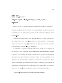
Abstract
MIMSY: A SYSTEM FOR ANALYZING TIME SERIES DATA IN THE
STOCK MARKET DOMAIN
In this thesis I describe a real{world application built on top of the CORAL
deductive database system. This application is meant to demonstrate the power of
CORAL not only as a deductive database but also as a generic extensible database
system. The application, Mimsy, is a stock market historical reporting system that
can answer questions about daily stock market pricing data. I will describe the
use of the Mimsy system, and issues related to its implementation.
vi
Chapter 1
Overview
'Twas brillig, and the slithy toves
Did gyre and gimble in the wabe:
All mimsy were the borogoves,
And the mome raths outgrabe.
{ Lewis Carroll , \Jabberwocky"
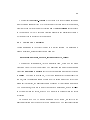
1.1 Introduction
CORAL [RSS92]is an extensible deductive database system developed at the University of Wisconsin. While providing all the functionality of a standard logic
programming environment like Datalog [CGT89], CORAL also provides the functionality of a general{purpose extensible database system [RSSS93b] .
CORAL provides two dierent operating environments. First, it provides an
interpreter capable of processing a declarative Datalog{like language. Second, it
provides an imperative environment where CORAL can be accessed from within
a host language. This environment is geared toward the building of non{trivial
database applications. The host language is C++ [ES90].
The rst non{trivial application built using the CORAL imperative environment is E XPLAIN [ARR+93]. E XPLAIN is a tuple derivation browser that
1
2
allows users to visualize the execution of a declarative query in CORAL for the
purposes of explaining the results of a query or to do \rule{level" debugging. In
eect, the user can determine which rules were responsible for putting which facts
in the database, or conversely, which rules should have put facts into the database,
but did not.
Though the notion of tracking which rules put which facts into the database
has wide applicability, E XPLAIN is mainly useful for people familiar with logic
programming or rule{based environments. The second non{trivial system built
on top of CORAL is Mimsy, a system for asking questions about stock market
data. Mimsy is the subject of this thesis. The raison d'^etre of Mimsy is twofold:
First, to show that a non{trivial application can be built using CORAL; second,
to develop an application that is useful in its own right.
An explanation of the name \Mimsy" is in order. The name was chosen for two
reasons. First, it was meant to be evocative of the Lewis Carroll poem included in
the epigraph of this chapter.1 Second, Mimsy is inspired by a commercial application sold by Logical Information Machines, Inc., called MIM2 [Lew92]. Mimsy is
meant to be thought of as an adjective meaning MIM{like. In lieu of a \Related
Work" section in this thesis, MIM should be thought of as the related work.
This is the way that MIM is described in its manual [Mac92]:
MIM allows a user to mine for nuggets of knowledge from the vast
1
2
Epigraphs for most other chapters are from [WT88].
Logical Information Machines and MIM are registered trademarks of Logical Information
Machines, Inc.
3
quantities of historical stock, commodity, economic and fundamental
data. This is done by constructing and executing ad hoc queries against
the historical data.3
This statement holds true for Mimsy as well. It should be noted that Mimsy is
at once both more powerful and less powerful than MIM. For example, MIM has
an extraordinary set of date primitives, whereas Mimsy has only a rudimentary
subset. However, MIM's range of extensibility is rather limited, while Mimsy's
extensibility has the full range of expressiveness of declarative CORAL, by virtue
of the fact that it has the entire CORAL system built in. Also, MIM provides
no way to deal with portfolios, whereas Mimsy allows portfolios to be used in the
same way as regular stock market data.
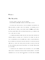
Mimsy consists of three parts. First, there is an interface that accepts queries
in the form of the Mimsy query language. Second, there is a translator the accepts
that Mimsy query and translates it into corresponding CORAL statements. These
statements are then sent to the Mimsy server. Third, the Mimsy server processes
the query and returns the answer back to the interface for viewing by the user.
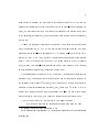
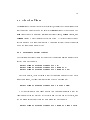
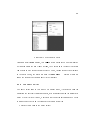
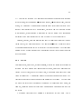
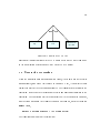
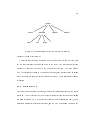
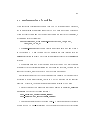
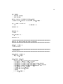
The design of the Mimsy system is shown in Figure 1.1. There are two basic
parts to the Mimsy system: the client and the server. The server consists of a
front{end that manages communication to the clients and a modied version of
CORAL. These modications include new data types and new types of relations.
The front{end manages communications between the clients and CORAL. The
communication between client and server is accomplished over Berkeley sockets
3
Used by permission.
4
Modification
to
CORAL
Server
Translator
Command
line
interface
Graphical
user
interface
Figure 1.1: The design of the Mimsy system
using techniques and publicly available source code described in [Ste90].
Mimsy clients consist of two parts. The rst part acquires a query in the Mimsy
query language from the user. The interface and the Mimsy query language are
described in Chapter 2. A graphical version of the interface, for use with the X
Window System, is described in Chapter 3. These two chapters are meant to serve
as a user's manual for the Mimsy system. The second part of a Mimsy client
is a translator that takes in a Mimsy query and translates it into its CORAL
equivalent. This is described in Chapter 4. The result of the translation is sent
to the server. After a query is sent to the server, which is described in Chapter 5,
5
the server's reply is sent back to the interface.
There are two main extensions to CORAL which exemplify one of CORAL's
major features: the ease with which CORAL can be extended. The rst is a new
data type that adds the ability to reason about portfolios. This will be described
in Section 2.7. The second extension is a new relation type optimized for use with
stock market data and its time{series nature. This will be described in Section
5.2.
1.2 Acknowledgements
First and foremost, I would like thank my advisor, Raghu Ramakrishnan, not only
for giving me the opportunity to be a Research Assistant and do this project, but
also for providing me support and encouragement along the way. Thanks also
go to Praveen Seshadri, who also provided support, both technical and otherwise.
Because of their involvement during the design process, this work is as much theirs
as it is mine. Special thanks to Eben Haber for his help in attening my learning
curve for InterViews. I would also like to thank Walt Ludwig, Nick Street and John
Cheevers for help with LaTEX. Thanks also go to Susan Hert for helpful comments
on an earlier draft of this work. Finally, I would like to thank my long{suering
wife, Mary, AKA the world's greatest proof{reader, to whom I owe about a year's
worth of washing dishes.
Chapter 2
The Language
Where the devil
should he learn our language? I will give him some
relief, if it be but for that.
Stefano to Trinculo { The Tempest II.ii(67)
In this chapter, a description of the Mimsy query language is given. The goal
is to provide an SQL{like language specically geared toward the application of
querying stock market data. I will rst provide an overview of the language in
Section 2.1. In Section 2.2 I will describe the command line interface to the query
language. In Section 2.3 I will discuss the graphing utilities available from the
command line interface. The Mimsy query language will be described in detail
in Sections 2.4 through 2.8. Mimsy query language extensibility is discussed in
Section 2.10. To close out the chapter, I will discuss the data used by the query
language in Section 2.11.
6
7
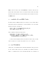
2.1 Overview of the Query Language
The basic structure of a Mimsy query is as follows:
select <something>
when <something-else>
save as <something-to-be-saved>
Both the when and the save
as
part of the query are optional. The select
clause determines what data will be returned to the user. The when clause determines for which dates the data in the select clause will be shown. The save
as
clause species that the answers should be projected into a relation instead of
displaying the results of the query on the screen.
The data operated on by Mimsy is known as a series. A series is a vector of
price data. A series can be thought of as a binary relation with the rst column
specifying the date or time index, and the second column specifying the value of
the series at that index. In Mimsy, a series is identied by its ticker symbol and
an identifying attribute. For example,
close of abc
represents the close series
for the stock whose ticker symbol is abc. The series used in Mimsy are cataloged
and described in Section 2.11.
Operations, known as aggregates, can be applied to series to produce values.
Some of the standard SQL aggregates implemented in Mimsy are average, min,
max,
etc. Aggregates and a time range are applied to base series. For example
the 30 day average of close of abc
represents the 30 day moving average of
the stock whose ticker symbol is abc. The aggregates and their denitions are
described in Section 2.6.
8
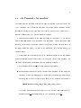
2.2 The Command Line Interface
The command line interface provides a means of entering Mimsy queries at the
UNIX command line. It provides command line editing and a command history
mechanism similar to the \tcsh" shell. This facility is achieved by using the GNU
readline [Fox91b] and GNU history [Fox91a] libraries.
All valid queries conform to the grammar found in Appendix A. Note that all
queries (and commands) are terminated by a semicolon. Once a query has been
received, the interface determines whether the string is a command or a query. If
the input string is a query, it is sent to the translator. If it is a command, it is
handled locally.
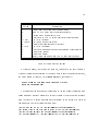
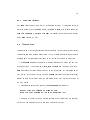
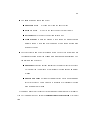
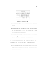
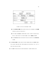
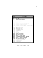
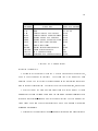
The command line interface to the Mimsy translator has only a few commands.
Besides executing queries that begin with the word \select" and \graph", the
command line interface understands the commands in Figure 2.1.
The denitions for the non{trivial commands are as follows:
Portfolios are created by using the \create" command from the command line
interface. It has two arguments: a string that represents the name of the
portfolio, and a list of the stocks to be added to the portfolio. For example:
create myport [[drv,1000,9.25],[adt,1000,12.5]];
will create a portfolio called \myport" with 2 stocks: 1000 shares of DRV
purchased at $9 41 , and 1000 shares of ADT purchased at $12 12 .
9
Command
Explanation
create
store
show
list
load
send
timing
history
quit
quit server
Create a portfolio
Save a relation or a portfolio
Show portfolios dened on server
List relation on sever
Load catalog information from server
Send an arbitrary string to the server
Toggle timing of commands at the server
Show the command line history
Quit the command line interface
Kill the server
Figure 2.1: Mimsy commands
The \store" command saves a relation or a portfolio so that it will be loaded
by the server the next time it starts up. To save the newly created portfolio
\myport," issue the following command:
store portfolio myport;
To save the relation \myrel" which was created by a query with a save
as
clause, issue the following command:
store myrel;
The \show" command lists all of the portfolios currently dened on the
server. The answer is returned to the interface.
The \list" command lists all of the relations currently dened on the server.
The answer is shown at the server.
10
The \load" command loads catalog information from the server. This information is loaded when the command line interface starts up, but a \load"
command will be needed if new portfolios, series or properties are dened.
The \history" command lists commands previously entered and illustrates
that the command line interface has a history mechanism similar to the
\tcsh" shell.
The \send" command allows the user to send an arbitrary CORAL string to
the server. Everything after the word \send" is sent to the server as it was
typed. For example, if the user wanted to display the CORAL defaults on
the server, the following command would be sent:
send display_defaults.;
There are several command line options available in the command line interface.
They are shown in Figure 2.1.
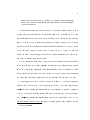
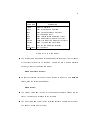
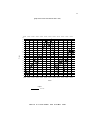
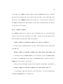
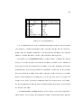
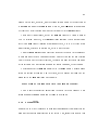
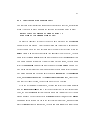
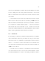
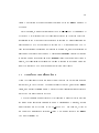
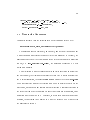
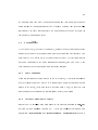
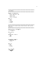
2.3 Graphing Utilities
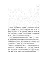
When a query is issued at the command line interface using the select keyword,
the output is sorted and displayed on the screen. However, if the graph keyword
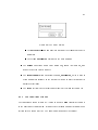
is used, the user will be presented with a graph. For example:
graph close of ibm when date is after "1/1/90";
11
graph close of ibm when date is after 1/1/90;
01/03/90
122
02/01/90
03/05/90
04/03/90
05/03/90
06/04/90
07/03/90
08/02/90
08/31/90
10/02/90
10/31/90
11/30/90
02/01/90
03/05/90
04/03/90
05/03/90
06/04/90
07/03/90
08/02/90
08/31/90
10/02/90
10/31/90
11/30/90
121
120
118
117
116
114
113
Prices
112
110
109
108
106
105
104
103
101
100
99
97
96
01/03/90
Dates
Legend
close of ibm
Figure 2.2: Typical output from a \graph" query
12
Option
Explanation
-C
-S
-T
-c
-f <le>
-h <host>
-n
-o <le>
-p
-q
-s
-t
Do not load tables from server upon startup
Show CORAL query that the parser generated
Testing mode. Equivalent to -qcn
Print query in CORAL print() statement before parsing
Use <le> for input
Use <host> as host for server
Do not send translated query to server
Use <le> for output
Print query and number of queries processed before parsing
Do not print prompt
Do not sort output
Insert timing commands into CORAL code sent to server
Table 2.1: Command line options
will cause a graph, like the one in Figure 2.2, to appear if the user is on an X
Window terminal or workstation. If the user wishes to save the PostScript output,
the query should be issued with the save
as
clause, for example:
graph close of ibm when date is after "1/1/90"
save as "filename.ps";
The PostScript for the graphics is generated by the IPL graphics program from
Johns Hopkins University School of Medicine [Gru90]. When the data is returned
from the server it is sorted and formatted for output to the screen by a series of
commands similar to the following command:
/usr/bin/sort -t/ +2n +0n +1n /usr/tmp/aaaa16579>/usr/tmp/caaa16579;
echo "graph close of ibm when date is after 11/1/90;">>/usr/tmp/caaa16579;
/usr/gnu/bin/gawk -f graph.awk /usr/tmp/caaa16579>/usr/tmp/daaa16579;
tipl /usr/tmp/daaa16579 > /usr/tmp/daaa16579.ps;gv /usr/tmp/daaa16579.ps
13
This string is constructed and executed by means of the system() system call.
The call to \gv" at the end of the string is a call to GhostView [The92], a PostScript
viewer for X Window system. When a \graph" query is executed, a GhostView
process is run in the background. This means more than one PostScript viewer
can be running at once.
2.4 The Select Clause
In the Mimsy query language the select portion of the language is comprised of
one or more select attributes separated by commas.
2.4.1 Select Attributes
A select attribute is composed of a select expression followed by an optional
repeated
clause. A select expression is a series, aggregate on a series, or an
arithmetic expression involving a series or an aggregate. Examples of the select
clause are shown below.
select close of ibm;
select 3 * close of ibm repeated for 10 days;
select the 4 day average of close of ibm + 1;
select close of ibm - close of ibm 1 day ago
repeated from the previous 2 days to
the next 3 days;
It should be noted that all series can be modied by an oset clause, for example
close of ibm 1 day ago
or close
of abc 2 days later.
If the oset clause
14
is used in conjunction with an aggregate, the oset applies to the aggregate being
applied to the series. For example,
the 5 day average of the close of ibm 3 days ago
means that 3 days prior to the date under consideration the 5 day moving average
of the closing price of IBM should be computed.
2.4.2 The Repeated Clause
A select attribute can be modied by a repeated clause in the select portion of
a query.
Repeated
clauses take 1 of 2 forms, as shown below:
select close of abc repeated from previous 10 days to next 10 days;
select close of abc repeated for the next 10 days;
There is also an alternate version of the latter form in which the \next" is implied:
show close of abc repeated for 10 days;
The eect of the repeated clause is that, for a given date returned from the
when
clause, the repeated clause causes the select attribute to be shown for all
dates in the range. A repeated clause takes precedence over any oset applied to
a select attribute. For example, in the query:
select close of abc - close of abc 1 day ago repeated for 3 days
when <some condition>;
For each date on which the when condition holds, the 1 day move of the close
of abc is shown for that day and for the next 3 days as well.
15
2.5 The When Clause
The when clause is meant to be a list of predicates, separated by logical connectives
that choose the dates for which the data in the select clause is to be shown. The
when
clause comes in 3 avors: relational operator clauses,
crosses
change
clauses, and
clauses. These clauses are described below. All of these clauses can be
further modied by a condition interval. A condition interval is a date range for
which the condition must hold true.
2.5.1 Relational Operator Clauses
The relational operator clause tests one select expression against another for a
specic date. For example:
select close of abc when close of abc > 12;
select close of abc when close of abc > close of b;
select close of abc when close of abc > close of b * 6;
For these queries, the implication is that the condition holds over 1 day. For a
longer date range, the condition interval can be used. For example:
select close of xrx when close of xrx > 12 over 3 days;
The implication of a date range applied to a relational operator is that the
condition holds for the rst day of the series and the last day of the series, and
the left argument does not cross the right argument. For example:
select close of abc when close of abc > close of b over 3 days
16
implies that the close
of abc
is greater than the close
of b
on the rst and
last days of the range, and that the prices do not cross. For a denition of the
semantics of the crosses clause, see Section 2.5.3. These semantics hold for all
relational operator except \not equals". In this case the operator must be applied
to every date in the range.
2.5.2 Change Clauses
The
clauses test whether a select expression is up or down over some
change
period. There are three versions of this clause. First, a select expression can be
checked against some xed amount. For example:
select close of abc when close of abc is up at least 10;
Second, a select expression can be checked against another select expression.
For example:
select close of abc when close of abc is up more than close of b;
This means that the close
is up and the
close of b
close of b
of abc
will be displayed when the close
is up and the
close of abc
of abc
is up more than the
is up over a 1 day period.
Finally, a select expression can be checked against a percentage. For example,
select close of abc when close of abc is up more than 10%;
The percentage gure can also be a select expression. There are also negated
versions of change clauses. For example:
17
select <something>
when close of x is not up
This means that close
the negated
change
of x
is down or unchanged over the interval. When
clauses are used with relational operators like \less than",
\more than",\at least", etc., the \not" applies to the operator. For example, the
query
select a when close of abc is not up more than 10;
means the close
of abc
should be displayed when the close
of abc
is up, but
not when it is up more than 10 points.
2.5.3 Crosses Clauses
The crosses clause tests when one series crosses another. A cross occurs when, for
example, one stock's price moves above the price of another when the rst stock
was smaller or equal in price to the second stock in the previous time period. For
example:
select close of abc when close of abc crosses close of b;
This query will select the close
crosses above or below the close
\above" or \below" in the
interest. For example:
of abc
of b.
crosses
on all dates when the close
of abc
The query writer can also specify either
clause to specify which type of cross is of
18
select close of abc
when close of abc crosses above
the 30 day average of close of abc;
The preceding query also illustrates that any select expression can be used as
the right or left argument to the crosses predicate.
However, it should be noted that any non{series (e.g. an equation, aggregate,
etc.) that appears as an argument to the
crosses
clause is rst be projected
out into a temporary relation. See Section 4.1 for more details. This is because
the
crosses
predicate in CORAL expects to operate on series. If a non{series
is present, one must be created beforehand by projecting out the appropriate
date/value combination. The only exception to this is if one of the arguments
is a numeric constant, e.g.
when close of b crosses 8,
whenever the value of the close
of b
which will return true
crosses the value 8. Also, in the presence
of a condition interval, the crosses clause will succeed if any crosses exist in the
range. There is also a negated version of the crosses predicate. For example:
select close of abc when close of abc not crosses close of b;
This means that the close
does not cross the close
crosses
of b.
of abc
will be displayed when the close
of abc
It should be noted that the negated version of the
predicate illustrates the fact that the negated crosses clauses makes use
of CORAL negation. This obviates the need for positive and negative versions of
the predicate in the CORAL translation. For a description of how this is translated,
see Section 4.6.
19
2.5.4 Condition Interval
Any
when
clause can be modied by a condition interval. A condition exists in
one of two forms; either an over clause, like over
3 days,
from the previous 3 days to the next 10 days.
or a relative range like
The default period for any
of the when clauses is 1 day.
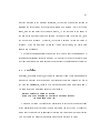
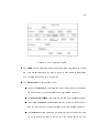
2.6 Aggregates
Aggregates in Mimsy are operations that are applied to either series or portfolios.
Aggregates compute a single answer from the time range and series that are given
as arguments. The aggregates included in the system are shown in Figure 2.2.
The
average
aggregate computes a moving average of a series for the time
period specied. The denition of
Move
min, max
and
sum
are the same as in SQL.
represents the total change in price of the series from the beginning of the
time period to the end of the time period.
Pcmove
represents the total percentage
change in price of the series from the beginning of the time period to the end of
the time period.
All aggregates are used as follows, using average as an example:
select the 5 day average of close of ibm
when the 3 day average of ibm is up more than 10%;
This query will show the 5 day moving average of the close of IBM on each day
when the 3 day average rises by more than 10 percent in 1 day.
20
#
Name
1
2
3
4
5
6
Average
Max
Min
Sum
Move
Percentage Move
Mimsy Aggregate name
average
max
min
sum
move
pcmove
Table 2.2: Mimsy aggregates
Mimsy aggregates are written to recognize opportunities for ecient execution.
This is done by having the aggregate cache its arguments and some of its computations from the previous invocation. Note that forward motion of time is always
assumed when an aggregate is being iterated across a range of dates.
For example, if the average aggregate is called on day 1 through day 20 of a
series, it will cache the number of days in the range, the name of the portfolio or
series, and the sum of the values over the range. If the next invocation is for day 2
through day 21 of the series, to compute the average it is sucient to get the value
for the previous lower bound of the range, subtract it from the sum, get the value
for new upper bound for the range, add it to the sum and divide by the number
of days in the series. If the next invocation is not for the next day in the window,
the cached values are discarded and the computation must proceed as if called on
the rst day of a range.
The aggregates min and max are optimized similarly. If either of these aggregates is called with the same date range, for the same symbol and for the next day
21
after the one used in the previous invocation, the call can be optimized instead of
scanning the entire range. If the previous minimum or maximum is still in the date
range, only the new point in the range is needed, i.e. the last date in the range. If
the new point is greater than the maximum (or smaller than the minimum), then
the new value is returned. Otherwise, the cached maximum (minimum) value is
returned. If the old maximum (minimum) is now out of range, the entire date
range must be scanned.
The eect of having aggregates optimized in this way is that the aggregates will
recognize all occasions for optimizations. This obviates the need for any higher
level optimizations other than sorting the data before the aggregates are executed.
2.7 Portfolios
Portfolios, or groups of stocks, are handled separately from series and aggregates
and have a dierent set of properties. Portfolios are specied through the use of
the keyword
portfolio,
followed by a portfolio property and a portfolio name.
An example of how portfolios are used is as follows:
select portfolio value of myport
when the 3 day average of portfolio value of myport
is down more than 10%;
This query will show the value of the portfolio \myport" when the 3 day average
of the portfolio value of \myport" is down more than 10% over 1 day. It should be
noted that the normal set of aggregates (Section 2.6) can be applied to portfolios.
This is because the property/portfolios pair behaves similarly to series.
22
There are currently two properties that can be applied to portfolios, value and
position.
The value of a portfolio is the sum of the prices for a particular day.
The position of a portfolio is the value minus the sum of the initial prices times
the initial quantities. This reects the value of the portfolio relative to the initial
prices.
2.8 Date Handling
Dates and specication of date ranges play a large role in the Mimsy query language. Section 2.8.1 covers the syntax of basic date selections. Section 2.8.2 covers
the two special date forms for specifying regularly occurring date conditions.
2.8.1 Basic Date Handling
Selections made by the
when
clause can be limited by dates as well. There are
currently four forms for specifying dates. First, a particular date can be specied;
for example, when
date is "1/2/90".
specied, for example; date
Second, an upper or lower bound can be
is after "1/2/90"
or date
is before "1/2/90".
Third, a date range can be specied; for example:
date is from "1/1/90" to "1/1/91".
There are several date units than can be applied to oset clauses and range
clauses. The following date units are available in Mimsy: day, week, month, year.
It should be noted that all dates supplied to the Mimsy query language must
23
be quoted strings. A description of the grammar for date strings can be found
Appendix B.
2.8.2 Special Date Form
There is a special form of the date condition that checks for a particular month
or day of the week. For example, if the user is concerned with all Fridays, the
following clause could be used:
when date is on "friday";.
If the user is only concerned with dates in March, the following clause can be used:
when date is in "march";
Note in these examples that quoted strings must be used to specify dates, as they
are passed directly to CORAL built{ins.
2.9 The Save As Clause
The
save as
clause has two semantically distinct uses in the query language.
First, it can be used to save the results of a query into a CORAL relation. For
example:
select close of abc save as new_series;
close of b * 3
This would create a new binary relation on the server called new_series. The
new relation would have as its rst column the dates for which the series was
24
dened (in this case, all dates), and the second column would be the dierence of
3 * close of b
and the close
of abc.
Likewise, a multi{column relation could
be created by merely having multiple select attributes in the select clause.
Under most circumstances, use of the
save as
clause will create a normal
CORAL relation. However, if the select clause contains 1 select attribute and
there is no
when
clause (insuring a contiguous series), Mimsy will create a fast
array relation, described in Section 5.2, which is more ecient.
Using the save
as
clause only stores the results of the query to the database.
It does not make the new relation persistent. In order to make the new relation
visible the next time the server starts up, the user must issue the \save" command
at the interface. For more information on the \save" command, see Section 2.2.
The second use of the save
as
clause is with the graph clause. To save a graph
into a le instead of showing it on the screen, merely provide a lename as the
argument to the save
as
clause. For example:
graph close of ibm when date is in 1990 save as "foo.ps";
This will save the PostScript output from the query to the le \foo.ps". More
information on the graph clause can be found in Section 2.3.
2.10 Extensibility
Extensibility in Mimsy is provided by allowing strings found at certain places in the
grammar to be passed uninterpreted to the server. Also, variables in a query that
25
refer to variables in extensibility strings are allowed to appear in select expressions.
Note that the rst letter of a variable must be in upper case. A special variable,
\Date", can appear in the argument string. In the translation, the string Date will
be replaced by the variable that represents the current date under consideration.
For example, suppose we had a predicate \extend" that returned some value. We
would use it like this:
select close of abc,"new_series(Date,Val)",Val
when "extend(Date,X)" and X > 12.
This query illustrates how extensibility is used in the
select
clause. If an
extensibility string is in the select list, it is not shown in the printed output. In
order to display the values of an extensibility string, the variables must explicitly
be put into the list of things to be displayed. For example:
select "a(Date,Test)", Test, close of ibm
when close of ibm is down more than 10%;
When extensibility strings are used in the when portion of the query, they are
considered actual when clauses and as such the variables used to refer to the strings
must exist in clauses that associate with them. An example of this is shown above
in the extend query. The variable X must be included in the extensibility string
before it can be referenced in the X
> 12
clause. To use this eectively, the user
must be aware of certain aspects of how the query is translated into CORAL. For
this information, see Chapter 4.
26
#
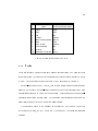
Name
1
2
3
4
5
6
7
8
9
10
Close
High
Low
Volume
Shares outstanding
Beta
Beta return
Capitalization
Return
Standard deviation
Mimsy Sequence name
close
high
low
volume
shares
beta
betaret
cap
ret
stdev
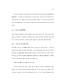
Table 2.3: Base series dened in Mimsy
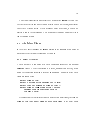
2.11 Series
There are currently 10 base series each dened for 165 stocks. The data for these
series comes from the University of Chicago's Center for Research in Security Prices
(CRSP). The series and their keywords in Mimsy are shown in Table 2.3.
Series 1{5 are base series. That is, they are are actual values describing some
property of the stock. Series 6{10 are composite series that represent some kind
calculation performed by CRSP on the base data. These composite series are pre{
calculated and stored as base data. The following descriptions are based on the
denitions provided in the CRSP data manual [iSP92].
The Beta of a stock is the measure of its volatility with respect to the rest
of the market [Mal85, EG91]. The Beta is dened by the following equation
[iSP92]:
27
P (ret mret3 ) ? ( 1 )(P ret )(P mret3 )
= P (mret mret3 ) ? ( 1 )(P mret )(P mret3 )
t
i;t
t
t
t
i
t
n
t
n
t
i;t
t
t
t
t
t
(2.1)
where:
ret = log10 (1+ return of security i on day t)
i;t
mret = log10 (1+ value{weighted market return on day t)
t
mret3 = mret ?1 +mret +mret +1 (a 3 day moving average market window)
t
t
t
t
n = number of observations for the year.
The beta return, also known as the \beta excess return" is the excess return of
a specic stock less the average return of all issues in its beta portfolio.
The capitalization of a stock is the price of the stock times the number of shares
outstanding. Usually, the price of the stock used in the calculation is the price at
the end of some xed time period. In the case of the CRSP data, the price used
is the price at the end of the previous year.
The return of the stock represents its gain (or loss) per $1 of investment from
the previous trading day.
The standard deviation of a stock is dened by the following equation [iSP92]:
qP 2 1 P
ret ? ( ret
=
n?1
t
i
where:
i;t
n
t
i;t
)2
(2.2)
28
ret = daily raw trade of security i on day t
i;t
n = number of observations for the year (of ret )
i;t
= yearly standard deviation for the i company.
i
th
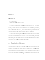
Chapter 3
The Graphical Interface
He had a face only a mother could love.
Unknown
The Mimsy system provides a graphical user interface to its query language.
The goal is to provide the user a means for constructing queries using only the
mouse. The interface, which is about 9100 lines of C++ code, was also built to act
like a graphical text editor so that users can copy and paste queries and the output
of queries to other applications running on a workstation. In this chapter, I will
rst discuss the layout and use of the interface in Section 3.1. I will conclude the
chapter with a discussion of issues related to the design of the interface in Section
3.2.
3.1 Use of the Interface
In this section, I will describe the basic use of the graphical interface. I will rst
describe how individual windows are used in Sections 3.1.1 through 3.1.4, and then
describe how an example query is constructed in Section 3.1.5.
29
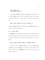
30
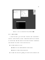
Figure 3.1: The Mimsy Interface at Application Start{up
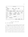
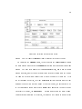
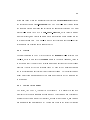
3.1.1 Main Window
As shown in Figure 3.1, the main window is displayed when the application is
started up. Its main function is to allow the construction of queries by bringing up
the attributes and condition windows via their respective buttons. It also handles
other functions via its menus. These are described below:
The File menu has two items:
{
About
{
Quit
which gives information about the application.
which causes the application to exit.
The Edit menu has one item, Undo, which allows the user to undo the last
31
clause added to the query.
The Query menu has one item, Clear
Query,
which clears the current query
from the query editor window.
The Utils menu has four menu items:
{
Reload Server Table
which reloads the database catalog information
from the server.
{
Set Host Name
which sets the host name for the host where the server
is running.
{
Send Arbitrary String...
sends an arbitrary string to the server un-
translated. This is useful for sending raw CORAL to the server.
{
Kill The Server...
sends the command to the server that causes it
to exit.
The Portfolios menu has three menu items:
{
Create Portfolio
brings up a dialog box to aid in the creation of a
new portfolio.
{
List Portfolios
{
Save Portfolio
will list all the portfolios the server knows about.
will save a portfolio on the server to a le, so that it
is loaded at server startup time.
There are three other interesting features to note in the main window. First,
there is the AND/OR pop{up menu to the left of the conditions button. When
32
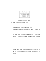
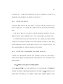
Figure 3.2: The Result of a Query
creating multiple
when
clauses, this pop{up menu determines which conjunctive
will appear before the new clause. Second, the Check Box in the lower left corner
can be used to time the queries on the server. Third, to send the query as displayed
in the query editor, the user must push the Send
Query...
button. Figure 3.2
shows the result of executing a query in the interface.
3.1.2 The Query Editor
The query editor runs in two modes. In display mode, it provides means for
displaying the currently constructed query, or a means for showing the output of a
query. When it is in edit mode, it acts as a text editor for entering queries. These
two modes have eects on the results of selecting a menu item.
There are two menus in the query editor:
33
The File menu has four menu items:
{
Read from File...
{
Write to File...
{
Edit Query
{
Close Window
will read a le into the query editor.
will write the query editor text out to a le.
puts the query editor into editor mode.
will close the window if the window is being used as an
output window. This menu item is disabled if this window is being used
as a query editor.
There are eight menu items in the Edit menu. The rst six menu items are
the standard editing menu items found on most graphical applications. The
remaining menu items are:
{
Send Query
sends the current contents of the query editor to the server.
This menu item is displayed if this instance is being used as an output
window.
{
Send As Raw CORAL will send the contents of the Query Editor untrans-
lated to the server. This menu item is displayed if this instance is being
used as an output window.
It should be noted that the facility to copy and paste is not one built into InterViews. It is accomplished by using the XStoreBytes and XFetchBytes Xlib[GS91]
calls.
34
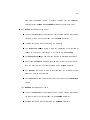
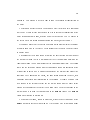
Figure 3.3: The Attribute Window
3.1.3 The Attribute Window
The attributes window (Figure 3.3) is used to add new select attributes (Section
2.4.1) to a select clause, or add operands to an expression. Once the clause is
constructed and the \OK" button is pressed, the new clause will appear in the
query editor. It contains seven sections that represent dierent types of select
attributes that can be used. Before setting up a new select attribute the user must
make sure that the radio button for the section that the user is interested in is
selected. A description of the seven sections of the attribute window are as follows:
35
Figure 3.4: The Oset Dialog
The Series section has the following items:
{ The Property pop{up menu for choosing properties on series.
{ The Series pop{up menu for choosing the series.
{ The Offset button for setting the oset to be applied to the series. An
example of the oset selection dialog box is shown in Figure 3.4.
{ The Repeat button for setting the repeated clause to be applied to
the series. An example of the repeat selection dialog box is shown in
Figure 3.5. This button is disabled if the window is adding an operand
to an expression.
The denitions for the
Aggregate
Offset
and
Repeat
buttons are the same for the
and Portfolio sections.
The Aggregates section has the following items:
{ The Time
Period
button brings up a dialog box similar to Figure 3.4
that allows the user to choose the time period to be applied to the
aggregate.
36
Figure 3.5: The Repeat Dialog
{ The Aggregate pop{up menu provides a list of currently available aggregates.
{ The Portfolios check box chooses whether the aggregates should act
on a portfolio or a series. This check box is primarily used in setting
up the Properties and Series menus.
{ The Properties and Series pop{up menus are similar to the one in the
Series
section, unless the Portfolios check box is checked in which
case the menus refer to portfolios and portfolio properties.
The items in the Portfolios section have similar denitions to the ones in
the Series sections. There are three items in the Math
Ops
section:
{ The rst Expression button brings up another instance of the attribute
dialog box to assist in setting the left operand to the arithmetic operation under construction.
37
Figure 3.6: The Entry Dialog
{ The MathOps pop{up menu provides a menu of the standard arithmetic
operators.
{ The second Expression button sets the right operand.
The Number box brings up an entry dialog box, shown in Figure 3.6, and
allows the user to enter a number.
The Parentheses section has a single button, Expression, which is used to
bring up another instance of the attribute window in order to construct a
parenthetical clause.
The Other section is used for entering extensibility strings (Section 2.10).
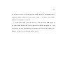
3.1.4 The Conditions Window
The conditions window (Figure 3.7) is used to add new when clauses (Section 2.5)
to the query under construction. It too uses a set of radio buttons to control which
section of the window is active. The condition window has six sections:
38
Figure 3.7: The Condition Window
The Dates section brings up a date selection dialog box, shown in Figure
3.8. This dialog box allows the user to set up a date clause in accordance
with the grammar described in section 2.8.
The Comparison section has four items:
{ The rst Attribute button brings up an Attribute window that allows
the user to select the left operand of the comparison operator.
{ The Operators pop{up menu provides a menu of relational operators.
{ The second Attribute button brings up an Attribute window that allows the user to select the right operand of the comparison operator.
{ The Interval button brings up a window similar to the one in Figure
3.5 which allows the user to specify the time period over which the
39
condition is supposed to hold. It should be noted that the Interval
buttons for the Change and Crosses sections are dened similarly.
The Change section has seven items:
{ The rst Attribute button brings up an Attribute window that allows
the user to select the left operand to the change operator.
{ The Not check box is used to negate the operator.
{ The Direction pop{up menu is used for displaying the direction of
change in which user is interested. The choices are Up and Down.
{ The Operator pop{up menu displays a menu of relational operators.
{ The second Attribute button brings up an Attribute window that allows the user to select the right operand of the change operator.
{ The Percent check box is used to indicate that the second attribute
should be used as a percentage.
{ The Interval button is dened similarly to the one in the Comparison
section.
The Crosses section has ve items:
{ The rst Attribute button brings up an Attribute window that allows
the user to select the left operand to the crosses operator.
{ The Not check box is used to negate the crosses predicate.
40
Figure 3.8: The Date Selection Dialog
{ The Crosses pop{up menu is used to select which version of the crosses
predicate the user is interested in.
{ The second Attribute button brings up an Attribute window that allows the user to select the right operand of the crosses operator.
{ The Interval button is dened similarly to the one in the Comparison
section.
The Parentheses section is used to create a parenthetical set of when clauses.
Note that the conjunct used between clauses is determined by the AND/OR
menu on the main window.
The Other section is used to input extensibility strings (Section 2.10).
41
3.1.5 Construction of an Example Query
Now that each of the interface's windows has been described in detail, a description
of how it works is in order. Suppose the user had the following query in mind:
select the 30 day average of close of sp500 / 2
when close of ibm crosses close of dec;
In order to construct this query the user would rst push the
Attributes
button in the main window. An attributes dialog box (Figure 3.3) would appear.
The user would select the type of clause that s/he would like to create. Since the
select
clause is an arithmetic operation (the aggregate is divided by 2), the user
would select the Math
Ops
radio button and then push the left Attribute button.
This would bring up yet another Attribute dialog. In this window, the user would
select the Aggregates radio button and then push the Time
Period
button. The
time period dialog (Figure 3.4) would appear and the user would select the 30 day
time period and push OK. The user would then select average from the Aggregates
menu, and close and sp500 from the Properties and Series menus, respectively.
Now that the clause is setup, the user can push the \OK" button.
With the left operand is constructed, the user can select the division operator
from the Operators pop{up menu. Next the user needs to ll in the right operand.
Thus, the right Attribute button is pushed and a new instance of the Attribute
window appears. The user then selects the Number radio button, pushes the Number
button and enters the number \2" in the entry dialog (Figure 3.6), and pushes OK.
Since the select clause is constructed, the user can push OK on the main attribute
42
Figure 3.9: Selecting a Property on Series
window. This will cause the select clause to appear in the query editor.
To construct the crosses clause, the user pushes the Conditions button on
the main window and selects the Crosses radio button on the resultant Conditions
window. The user then pushes the left Attribute button, and a new attribute
window appears, and the correct property and series are chosen from the menus.
An example of selecting a property on a series is shown in Figure 3.9. After
the left operand is selected, the right Attribute button is pushed and the right
operand is selected in a similar manner. When this is done, the user pushes \OK"
in the conditions window and the new
To execute this query, the Send
when
Query...
clause appears in the query editor.
button is pushed on the main window.
Upon successful execution by the server, the results will be shown in a query editor
43
in display mode, similar to Figure 3.1.
3.2 Interface Design
In this section, I will cover topics related to the design of the interface. In Section
3.2.1, I will give a brief overview of InterViews, the graphics package that was
used to build the interface. In Section 3.2.2, I will give a brief description of
how InterViews and its interface builder are used. To close out the chapter I will
provide some comments on the design of the interface in Sections 3.2.3 and 3.2.4.
3.2.1 InterViews
The basic platform upon which the Mimsy graphical interface is built is InterViews
[LVC89]. Developed at Stanford University, it is a set of tools and a library of
C++ classes that assist in the design and implementation of graphically interactive
applications. InterViews' class library provides a high{level abstraction for dealing
with graphical user interface objects, like scroll bars, push buttons, interface text
windows, etc. It provides specic support for resolution{independent graphics,
and a graphical tool to build user interfaces interactively [LCI+ 91]. InterViews is
currently implemented on top of the X Window system [SG86].
3.2.2 Typical Use of InterViews
Typically, user interfaces are constructed in InterViews using the
ibuild
tool.
The developer rst constructs the interface graphically, and then generates the
44
C++ code for the interface. The generated code handles the normal user interface
sets of actions, like resizing and re{drawing windows, hi{lighting buttons, drawing
menus, etc.
Ibuild
will also generate function stubs for actions that need to be
taken by user interface objects. For instance, for each menu item and each button
in an interface, a function stub is generated so that the action to be taken upon
activation of the user interface object can be coded by the developer later.
Ibuild,
however, does not generate any code to handle anything that is appli-
cation specic, like drawing graphics. Any application{specic behavior is coded
by subclassing an existing object in the InterViews class hierarchy. The signicant
portion of time writing an InterViews application is spent in writing methods for
these subclasses.
3.2.3 Design
To a large degree, InterViews, or rather ibuild, dictated the design of the graphical
interface. For each window that appears on the screen, InterViews generates two
classes. The rst class, called the \core" class, is a subclass of an InterViews class
called a MonoScene. A MonoScene denes the basic operations of a window. The
core class denes the default behavior of components of the window. The core class
is where most of the code is generated by ibuild. This generated code would, for
example, contain methods to create push buttons and menus and place them on
the screen.
The second class created by
ibuild
is a subclass of the core class. This is
45
where all the modications to the default behavior of components of the window
are made.
Ibuild,
as was stated above, generates function stubs. These stubs are
usually the action routines that are executed when a button is pushed or a menu
item is chosen.
The main concept driving the design of the interface has been that the interface
should mirror the behavior of the grammar. For example, a non{terminal in the
grammar indicates a recursion into some other part of the grammar. Graphically
this is represented by bringing up another window. A terminal in the grammar
would represent some kind of input from the user. An example of this occurs
when a user is constructing an arithmetic expression and nally needs to input a
number. For this, a dialog box is put up for entry of the number.
3.2.4 Class Design
In this section, I will describe the layout of the class structure in the interface.
When the application is started up, two windows are visible, the main window
and the query editor. The appearance of the application at startup is shown in
Figure 3.1. The window to the right is an instance of the MainWindow class.
The window shows the general outline of the query and is meant to represent the
\top{level" of the grammar.
The window to the left in Figure 3.1 is an instance of the QueryEditor class.
The QueryEditor has two modes. First it acts as a means of displaying the query
as it has been constructed by the user. In this mode, editing of the query is
46
disallowed. This window is merely meant to show the progress of construction of
the query.
The second mode for the query editor is one where it acts like a fully functional
text editor. It does this for those users who wish to forego the construction of the
query through normal means, or users who wish to send raw CORAL queries to
the server. For more information on sending raw queries, See Section 3.1.
It should be noted that the QueryEditor class is also used to display the output
of queries submitted to the server. These instances of the query editor act solely
in display mode.
One purpose of the main window is to allow the user to bring up two windows:
the attribute window (which is an instance of the AttributeDialog class) and the
conditions window (which is an instance of the ConditionDialog class). The reason
that both the attributes window and the conditions window are subclasses of the
Dialog class in InterViews is because subclasses of the Dialog class behave like
functions. They appear on the screen, get some information from the user, then
disappear and return that information to the program. It should be noted that
all windows in the interface except for the main window and the query editor
window are subclasses of the InterViews Dialog class. The other purpose of the
main window is to allow the construction of the
save as
clause. The
save as
clause was discussed in Section 2.9.
The attributes window, shown in Figure 3.3, allows the user to add any of the
select
attributes described in Section 2.4.1 to the query. One thing to note about
47
the attribute window is that each button therein labelled \Expression" actually
brings up another instance of the attribute window. This is how the recursive
nature of the grammar is reected.
The conditions window, shown in Figure 3.7, is used for adding when clauses to
the query under construction. These clauses were discussed in Section 2.5. Note
this window not only also brings up new instances of the attribute window, but
also new instances of the condition window as well.
Chapter 4
The Translator
Bless thee, Bottom, bless thee. Thou art translated.
Peter Quince to Bottom { A Midsummer Night's Dream III.i(113)
Once a query has been received by either the command line interface or the
graphical interface, the string is sent to the translator. The translator, which is
about 7500 lines of C [PB89], is implemented using a bison{based [DS91] parser.
If the query string acquired from the interface parses correctly, it is translated into
CORAL and sent to the server.
The translator maintains a global structure which keeps track of interface options and pointers to its output les. One such le is the output le where the
CORAL translation of the Mimsy language query is placed. Upon successful parsing, the contents of the output le are read and sent to the server over a socket
connection. The result of the query, when received from the server, is read from
the socket and sorted, and then either displayed at the terminal or graphed using
the IPL package.
The overall task of the translator is simple: generate CORAL for the
when
clause so that all its results are collected into one temporary relation. This relation
corresponds to the list of all dates that48satised all the conditions in the
when
49
clause. This relation is then used generate dates on which the select clauses will
be shown.
In this Section, a number of features of the Mimsy{to{CORAL translator will
be covered. Optimizations that the translator performs on the intermediate representation of the Mimsy query are described in Section 4.1. Issues regarding the
generation of CORAL are discussed in Section 4.2. A discussion of how CORAL
code for expressions is generated is discussed in Section 4.3, and the generation of
aggregates is discussed in Section 4.4. Generation of repeated clauses is discussed
in Section 4.5 and the generation of the crosses clause is discussed in Section 4.6.
Finally, the translation of extensibility strings is covered in Section 4.7 and the
chapter is concluded with a discussion of optimizing date clauses.
4.1 Translator Transformations
When the translator receives an input string it parses the string into abstract
syntax trees, or ASTs [ASU86]. The parser produces two ASTs, one for the select
clause, and one for the when clause. There are several transformations performed
on the ASTs in order to optimize them.
The rst transformation performed is to transform a property/series pair into
the name of the fast array relation to which it corresponds. Currently, all fast
array relations are of the form SYMBOL PROPERTY. For example, \close of
ibm" would be transformed into \ibm close." This is done for both the select
AST and the when AST.
50
The second transformation involves date ranges in the
when
clause. Since a
date range, e.g. \when date is from \1/1/80" to \1/1/90", represents a limitation
of the selectivity [SAC+ 88], the date range clause is moved as far toward the top
of the AST as possible. This is the equivalent of moving the date range clause to
the beginning of the CORAL statement and has the eect of limiting the dates
under consideration and narrowing the facts that must be iterated over.
The third transformation performed by the translator involves extracting expressions and creating series. This is needed for the crosses clause if its arguments are not series. The non{series arguments are projected into a temporary
relation and the temporary relation will be substituted for the expression. Note
that the expression extracted from the crosses clause will be dened across all
dates. Therefore, the temporary relation created will be a fast array relation.
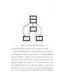
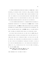
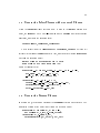
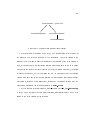
In the case where there are multiple ANDs and ORs in the when clause, the
translator attempts to optimize the generated code by putting as many AND
clauses into a single CORAL statement as possible. The eect of this is to have
the leftmost CORAL clause provide limitations on the selectivity of the clauses to
the right. It does this by collapsing the AST output by the parser. The eect of
this is that if the translator nds an AND AST with no children whose parent is
also an AND AST, it elevates the child AND AST to the parent. For example,
the AST for the when clause:
when close of abc is up and close of b > 12
and close of c is up more than 4%"
would correspond to the AST shown in Figure 4.1.
51
close of A is
up
close of B
> 12
close of C is
up > 4%
Figure 4.1: Unoptimized AND ASTs
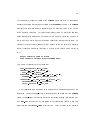
In order to optimize this AST the tree must be rearranged and group all ANDs
that associate together on the same level must be grouped together. The optimized
AST is shown in Figure 4.2.
4.2 Generating CORAL
After the transformations have been applied to the ASTs, the ASTs are passed
to the code generator which translates the ASTs to CORAL. In generating code
for the when AST, the code generator follows a simple algorithm. The format of
the
when
AST will be a tree of AND and OR nodes. If the generator nds an
OR clause, it generates each branch on its own line. The result of each statement
is projected into a temporary relation. If the generator nds an AND clause it
52
close of A is
up
close of B
> 12
close of C is
up > 4%
Figure 4.2: An optimized AND AST
generates all clauses contained in the AND clause (there may be more than 2 due
to the optimization described above) on 1 line of CORAL output.
4.3 Generating Expressions
When the translator nds an expression in a clause, it rst pulls out all the series
and aggregates, and binds their values to variables. Next, it substitutes those
variables in place of the series and aggregates. The translator next generates the
expression. It does so by rst generating the series and aggregates contained in the
expression. The expression itself is then generated with the substituted variables,
and the result is assigned to yet another variable. For example, given the following
select
clause,
select 3 * close of sp500 / 12 + close of ibm;
The translator would output the following:
53
?sp500_close(__D,__T0),ibm_close(__D,__T1),
__D0 = 3.000000 * __T0 / 12.000000 +
dateuntranslate(__D,__DATESTRING),
print(__DATESTRING,__D0),fail.
__T1,
4.4 Generating Aggregates
Aggregates currently take the following form when translated into CORAL:
seqaverage(BDate,EDate,SeriesOrPortfolio,Answer).
The aggregate takes a begin date, an end date, and a symbol indicating what
it is operating on and returns the answer in the last argument. By default, the
aggregate behaves as if it were acting on a series. If the 3rd argument is a function
symbol, e.g.
port_position(ibm_close),
the aggregate behaves as if it were
acting on a portfolio.
This distinction is made because properties on series are stored as a single array. For example, the closing price data for the stock ABC is stored as a single array. During translation, the phrase close
of abc
becomes the symbol abc_close
which represents the name of the relation from which to obtain the data. On the
other hand, portfolios do not contain any data; instead it contains references to
the series that comprise the portfolio. In order to get data out of a portfolio, some
operation must be applied to it. Therefore, in order for a portfolio to have any
meaning, the operation to be applied to it must be included with it in order for
the aggregate to act on it.
54
4.5 Generating Select Clauses with Repeated Clauses
When the
repeated
clause (Section 2.4.2) is used in the
query, the foreach CORAL built{in function is used.
select
Foreach
portion of a
acts like a sequence
generator, and takes the following form:
foreach(Result,Lowerbound,Upperbound).
Given integer input to
Lowerbound
and
Upperbound, foreach
will bind all
integers in that range to Result one at a time, and fail after binding Upperbound.
For example following query:
select close of abc repeated for 10 days
when close of abc is up more than 10%;
would be translated to:
whendates0(__D) += abc_close(__D,__D0),__T0 = __D + -1,
abc_close(__T0,__D1),__D0 > __D1,
__D0/__D1 > 1 + 10.000000 /100.
?whendates0(__D),__T0 = __D + 10,
foreach(__T1,__D,__T0),abc_close(__T1,__D0),
dateuntranslate(__T1,__DATESTRING),
print(__DATESTRING,__D0),fail.
4.6 Generating Crosses Clauses
In Section 2.5.3, the negated version of the crosses predicate was described. The
translated version of the query in Section 2.5.3 is shown below:
whendates0(D) += dates(D),D1 = D + -1,
not crosses(D1,D,both,a_close,bclose).
?whendates0(D),a_close(D,D0),
dateuntranslate(D,X),print(X, D0),fail.
55
As stated above, negated versions of the crosses clause use CORAL negation as
opposed to dening a new negative version of the crosses predicate. The crosses
predicate can also take numeric arguments, so the user can query to see when a
series crosses a threshold. This particular feature could be useful for someone
doing fundamental analysis or a \chartist" attempting to determine whether or
not a piece of a series has the \head and shoulders" characteristic[Mal85]. To
illustrate the above points, suppose a user wanted to see the value of a portfolio
when it crossed a particular threshold. The user might enter a query similar to
this:
select portfolio value of myport
when portfolio value of myport crosses 80000;
This would be translated to the following:
fast_rel(temprel0,sp500_close).
temprel0(__D,__D0) += dates(__D),
port_value(__D,myport,__D0).
whendates0(__D) += dates(__D),__T0 = __D + -1,
crosses(__T0,__D,both,temprel0,80000.0).
?whendates0(__D),port_value(__D,myport,__D0),
dateuntranslate(__D,__DATESTRING),
print(__DATESTRING,__D0),fail.
This translation also illustrates an important optimization undertaken by the
translator. Whenever a non{series is encountered as an argument to a crosses
clause, the non{series is projected out into a fast array relation (See Section 5.2).
The
fast_rel
predicate at the beginning of the translation creates a new fast
array relation using sp500_close as a template. Then the value of the portfolio
56
myport
is projected into the new relation temprel0. It should be noted that this
does not provide any speedup since all the relation accesses inherent in accessing
a portfolio that are now done in the projection would have been done in the body
of crosses anyway.
4.7 Translation of Extensibility Strings
In Section 2.10 query language extensibility is described. There is no real translation for an extensibility string passed to the query language. It is merely passed
through to the output. For example:
select close of abc,"new_series(Date,Val)",Val
when "extend(Date,X)" and X > 12.
would be translated into something similar to:
whendates(D) += dates(D),extend(D,X),X>12.
?whendates(D),a_close(D,D0),new_series(D,Val),D1=Val,
dateuntranslate(D,X),print(X,D0,D1).
The only thing of consequence done to extensibility strings is that the string
\Date" is replaced by the current date variable in the CORAL statement.
4.8 Date Optimization
Whenever the Mimsy translator sees a date range condition in a query, it attempts
to move this date range as near to the beginning of the translated output as
possible. The reason for this is that date range conditions limit the number of
57
dates that the conditions must iterate over. Also, the translator recognizes and
optimizes implicit date ranges. For example, given the following query:
select the close of abc
when date is after "1/1/90" and before "1/1/91";
the translator turns this into a query similar to:
select the close of abc
when date is from "1/1/90" to "1/1/91";
The translator then takes this new clause and optimizes it in the manner described
above.
Furthermore, recognizing that Mimsy dates are stored as integers, the translator inserts an iterator,
foreach,
that produces only the dates from the lower
bound to the upper bound for the range. This signicantly reduces the number of
times the when conditions must be executed and also limits the number of times
that relations will be accessed unsuccessfully.
Chapter 5
The Server
He is justly served.
Laertes to Hamlet { Hamlet V.ii(279)
The server is constructed as a front{end to imperative CORAL. As a result
of this, it has the entire CORAL interpreter built in. Operationally, the server,
which is about 8800 lines of C++, merely listens to a socket, consults whatever
comes over the socket and returns the result back to the originator.
The server is an iterative, connection{oriented server [Ste90]. The server is also
where the major extensions to CORAL exist. A new type of relation, called a fast
array relation, has been added and all of the series aggregates have been coded
directly as CORAL built{ins for performance reasons.
5.1 Organization of the server
The server expects to nd all of its data and start{up les in the server directory
hierarchy. The location of the server directory is determined by the pre{processor
macro LIBDIR or by the path associated with the \-l"option of the server. Both of
these set the global variable LibraryDir. The organization of the server directory
58
59
mimsy
mimdata
server
high
low
close
regrels
fastrels
...
Figure 5.1: Organization of the Server Directory Hierarchy
hierarchy is shown in Figure 5.1.
The server expects to nd its startup le in the \server" directory. This includes
the le that contains the denition of all of the series. The stock data directory
hierarchy is expected to reside in the \mimdata" directory. Any user dened
CORAL relations are found in the \regrels" directory, and any fast array relations
that were saved are expected in the \fastrels" directory. These relations are loaded
at startup.
5.1.1 Server Start Up
To set up the operation of the server, a number of things happen when the server
starts up. The le \servinit.F" in the server directory determines what operations
are done at startup time. The server rst loads the date translation table, which
translates regular dates into date integers, and the CORAL program to handle the
60
date osets. Next, the server loads in the relation that denes the catalog of all
base relations, and initializes all the base relations. The server then creates the
dates
relation, which is an unary relation that contains a date integer for every
valid date in the system.
In the next step, the server loads in semantic information that will be used by
both the command line interface and the graphical interface. This includes the
currently dened series, properties of series, portfolio properties, aggregates, etc.
This information is included in two les that are found in the \server" directory
in the server directory hierarchy. The les create catalog relations that dene
the above properties. The rst le, \semantics.P," is the module that projects
out all the portfolio names, series (by ticker symbol), and series properties. The
second le, \semantics.F," explicitly denes the current aggregates and portfolio
properties.
Finally, the server loads the information that denes the portfolios by consulting the le \load portfolios.F." This denes the portfolio schema by creating
all the portfolios through calls to the
create_portfolio
CORAL built{in and
assigning the result to the portfolio relation.
5.2 Fast Array Relations
One of the classic problems of dealing with stock market data is that it does
not t into the relational model very well. In the relational data model, every
\object" is treated as a table of an unspecied (though potentially large) number
61
of columns. The cost of maintaining this generality often makes accessing stock
market, and indeed all time{series, both time and space inecient. Some Wall
Street investment banks have even been known to use environments geared toward
dealing with vectors and matrices for their historical stock market data, like APL
[GR84, Ive62], and eschewing the use of RDBMSs completely.
In order to allow CORAL to operate eciently on time{series data, a new type
of relation has been added to CORAL which facilitates fast access of sequence data.
FastArrayRelation is a subclass of the CORAL class Relation and was added to
the CORAL class hierarchy by overriding three methods and the constructor.
A lename is passed to the FastArrayRelation in the constructor which species
the location of the data le. The data is loaded into the le the rst time the
relation is iterated over. The data is stored in the le as a binary array, so that
it can be loaded directly into memory without any translation. It is assumed that
the data in the le is in the host machine's numeric format.
A FastArrayRelation can be either unary or binary. When the relation is unary,
the only allowable form is to have its argument unbound and to be of type integer.
This form is primarily used as a sequence generator, that is, to generate a set of
contiguous integers to act as an index for binary FastArrayRelations.
Binary FastArrayRelations handle sequences. The class name for binary FastArrayRelations is \BinaryFastArrayRelation." The rst column is an integer
index. The second column is the value for that index, and is either a double precision oating point number or an integer. The rst column of the relation is not
62
actually stored. When the data is loaded, the header information, described below,
contains the number of elements in the array and the lower bound. From this, the
rst column can be synthesized. It is assumed that binary FastArrayRelations are
read{only, since the stock data is relatively static.
There is a specialized type of binary FastArrayRelations which allows inserts.
It is called an InsertableBFARelation. These relations are created by the fast_rel
built{in, which is described in Section 4.6. It is primarily used for creating fast
intermediate relations used by translated queries.
The second column is retrieved by a simple C++ array access. Also, CORAL
built{ins that are aware of FastArrayRelations can use the C++ method:
FastArrayRelation::operator[](int i)
to access the data in the relation without having to open a scan descriptor and
use the more common but more expensive method of iterating across tuples.
Each of the types of fast array relations is actually a C++ class. The FastArrayRelation hierarchy is shown in Figure 5.2.
5.3 The Schema Relation
When the server starts up, it loads a CORAL relation named sequence_schema.
A tuple in this relation looks something like:
sequence_schema(sp500,close,"").
63
FastArrayRelation
UnaryFastArrayRelation
(abstract class)
BinaryFastArrayRelation
InsertableBFARelation
Figure 5.2: The FastArrayRelation class hierarchy
The rst column is the name of the series. The second column is the name of
the property by which this sequence will be recognized. The third column is the
name of the le to load in order to instantiate the relation. If the third column is
null, this means that it is a fast array relation and should exist in the \mimdata"
directory in the server directory hierarchy. If the third column is not null, the string
is passed to consult(), which then loads the le. It is assumed that the relation
created from each line in the schema relation will have a name that consists of the
rst column, followed by an underscore, followed by the second column. For the
case shown previously the relation generated is sp500_close.
After the schema relation is loaded, a user{dened built{in, init_sequences,
is called which initializes the fast array relations, and consults any CORAL les
found in the third column of the relation.
64
5.4 Implementation of Portfolios
While fast array relations have shown that CORAL relations can be extended,
the implementation of portfolios shows that CORAL data types can be extended.
When a \create" command like the one in Section 2.2 is sent to the translator, it
is translated into the following:
portfolio(myport,X) += create_portfolio([[drv,1000,9.25],
[adt,1000,12.5]],X).
The
create_portfolio
predicate creates a portfolio data type and binds it
to the variable X. X and the name of the portfolio are then inserted into the
portfolio
relation as a tuple. Note that all portfolios are stored in the portfolio
relation.
The portfolio data type is implemented as a list of triples. The triple consists
of a pointer to the relation containing the price data for the stock, the number of
shares of the stock, and the price at which the stock was bought.
Portfolios are aware of the type of relations they contain. This means that if
a relation is a fast array relation, tuples in it will be accessed via the shortcut
provided. Otherwise, the usual means of accessing a relation will be used.
There are currently two properties that can be applied to portfolios, position
and value. They are of the following form:
port_value(Day,PortfolioName,Answer).
port_position(Day,PortfolioName,Answer).
All portfolio properties have the prex \port ". These properties are currently
written as CORAL built{in functions. These properties behave by rst retrieving
65
the portfolio data type from the portfolio relation and then applying the appropriate actions to the portfolio data type. It should be noted that these built{in
functions act as cover functions since the portfolio data type has methods for
computing its position and value.
5.5 Extensibility
At the lowest level, the server is extensible, because the user can send arbitrary
strings to the server via the \send" command in the command line interface. This
allows any CORAL statement to be executed on the server. This section discusses
more how extensions to the query language are handled, and how CORAL has
been extended in the server apart from fast array relations.
5.5.1 Query Language
When an extensibility string is used in a Mimsy query, it is placed unchanged
into the translated output. Since Mimsy cannot know about all relations that are
dened to the server, there is no validity checking done. Thus, it is expected that
a user who uses the extensibility feature knows what s/he is doing.
5.5.2 Current Extensions to Mimsy
Several CORAL built{ins have been added to the server in addition to fast_rel
(Section 4.6) and
translation:
foreach
(Section 4.5). There are built{ins that handle date
datetranslate
and
dateuntranslate. Datetranslate
takes in a
66
string and turns it into the appropriate date integer.
the inverse operation.
Init_sequences
Dateuntranslate
performs
is a CORAL built{in that iterates across
the sequence schema and loads and initializes the appropriate schemas. The nal
user built{in added to CORAL is fast_unary_relation, which takes in a name
and two integers, and creates an unary FastArrayRelation whose bounds are the
two integer arguments. This built{in is used for creating a fast space{ecient
relation used for iterating over a range of dates.
5.5.3 Crosses
The nal extension to CORAL in the server is the crosses built{in relation. This
built{in, which implements the
crosses
clause in the query language, takes in
two symbols that it expects to be relation names and succeeds for the date range
provided if prices of the two relations cross. It does this by opening scans on
the two relations and succeeding if any crosses are found. This predicate knows
about FastArrayRelations and uses this knowledge to optimize the scans on the
two relations.
5.5.4 Adding to the Server
The server, like CORAL, is meant to be extensible. It is possible to add new
predicates to the query language as shown above. Users can add new relations by
issuing the save command at the interface, as shown in Section 2.2, and can add
new aggregates and portfolios as well. Adding new series to the server is discussed
67
in Section 5.5.5. Adding new portfolios to the server is discussed in Section 5.5.6,
and adding new aggregates is discussed in Section 5.5.7.
5.5.5 Adding New Series
Users can dene series in one of two ways. First, new data can be added to the
server. Second, a CORAL module can be loaded into the server that denes a new
series.
Data can be added to the server by placing a properly formatted le in the
proper directory. For a discussion of the CORAL data layout, see Section 5.6.2.
To add a derived series to the server via a CORAL module, the module should
be placed in the \server" directory in the server directory hierarchy. In both cases,
information about the new schema should be added to the sequence schema. For
more information on the sequence schema, see Section 5.3.
5.5.6 Adding New Portfolios and Portfolio Properties
Creating new portfolios and making them persistent is described in Section 2.2.
To add a new property on a portfolio, the user denes a CORAL predicate of the
following form:
port_newprop(Date,Portfolioname,Answer).
where Portfolioname is the name associated with the portfolio in the portfolio
relation. Note that all portfolio properties have the prex \port " followed by their
lexical value. For example, if we wanted to dene a new portfolio property which
68
module port.
export port_sqrt(bbf).
port_sqrt(D,P,Ans) :- port_value(D,P,X), pow(X,.5,Ans).
end_module.
Figure 5.3: CORAL module dening the square root of value of a portfolio.
returned the square root of the value of the portfolio and we wanted to refer to
this property by the name \sqrt", the name of the new portfolio property would
be \port sqrt".
There are two ways to add a new portfolio property. The rst is to code the
new property as a CORAL built{in and compile it into the server. The description
of how to write CORAL built{ins is outside the scope of this thesis. For more
information on writing built{ins, see [RSSS93a].
The second way to add new portfolio properties is to add CORAL modules to
the server. The CORAL module for the square root of a portfolio's value is shown
in Figure 5.3. This module le would be placed in the \server" directory and an
entry to the semantics les would be added so that the clients can know of its
existence. The le must also be consulted. The best way to do this is to add a
line to the semantics le to consult the new module. Currently, there is no way to
iterate across the values of all of the individual stocks in a portfolio. In the future,
a new CORAL built{in will be provided which will be dened as follows:
portfolio_iterate(PortfolioDataType,RelationName).
69
The predicate portfolio_iterate will be called with the rst argument bound
and the second argument free. It will succeed once for each stock in the portfolio,
binding the symbol identifying the relation name to RelationName for each stock
in the portfolio. This will facilitate creating properties for portfolios because it
will allow access to all stocks in the portfolio.
5.5.7 Adding New Aggregates
Adding aggregates to the server is done in a similar fashion. An aggregate is
dened as follows, using \average" as an example:
seqaverage(BeginDate,EndDate,SeriesORPortfolio,Answer).
The names of all aggregates, in their translated form, begin with the prex
\seq" and end with their lexical value. The aggregate computes the appropriate
value from BeginDate to EndDate for the series or portfolio and returns the result
in Answer. As stated in Section 4.3, if the third argument of the aggregate is a
symbol, then the aggregate should behave as if it is acting on a series. If the third
argument is a functor, the aggregate should behave as if it is acting on a portfolio.
As with portfolios, there are two ways to dene new aggregates, as new built{ins
to be compiled into the server, or as CORAL modules to be loaded into the server
at startup.
To dene a new CORAL module aggregate to the system, an entry to the
aggregate relation must be added to the le \semantics.F". The aggregate relation
70
serves to dene the list of all aggregates available to the system. Additionally, a
line to consult the le must be added.
5.6 The Data
This sections describes the data that is used by Mimsy. Section 5.6.1 describes
the format of the original data. Section 5.6.2 describes the format of fast array
relation data and how to get it into that format from the CRSP le format.
5.6.1 Format of the Original Data
The data in the current Mimsy system comes from the University of Chicago's
Center for Research in Security Prices. Mimsy uses a subset of this data. The
format of the data (called the \stock" format) in its original form is shown in
Figure 5.1.
The format of the S&P 500 le is a little bit dierent. Its layout is (with
FORTRAN equivalents) is show in Figure 5.2.
5.6.2 Formatting the Data
Assuming that dates are in the formats specied above, there are two GAWK
[RF89] scripts that can be used for data conversion.
The rst script is \partition.awk" which takes as input a le in the \stock"
format. A variable named \dir" is dened in the script that points to where the
data les will be placed. For each stock, it creates a single le for each column of
71
Column
Field Name
1-8
9-13
14-18
19-23
24-28
29-33
34-38
39-43
44-51
52-62
63-73
74-84
85-96
97-109
110-121
122-133
134-145
146-151
152-156
157-163
164-179
180-191
192-203
CUSIP
number of observations
start date index
Exchange Listing Code
SIC Code
Number of Distributions Structures
Number of Shares Structures
Number of NASDAQ Information Structures
Date (YYMMDD)
Bid or Low Price
Ask or High Price
Closing Price
Volume
Return
Shares Outstanding
Beta Excess Return
Std Dev Excess Return
Capitalization Portfolio Assignment
Std Dev Portfolio Assignment
Beta Portfolio Assignment
Year End Capitalization
Annual Std Dev
Annual Beta
Table 5.1: CRSP Stock le layout
72
Columns
Field Name
1-6
7-20
21-34
35-48
49-62
73-78
79-84
85-100
101-106
107-114
115-128
Date
Value-weighted with dividends
Value-weighted without dividends
Equal-weighted with dividends
Equal-weighted without dividends
Total market value in $1000
Total market count
Market value of securities used
Count of securities used
S&P Composite Index
Return on S&P Composite Index
FORTRAN Format
YYMMDD
E14.6
E14.6
E14.6
E14.6
E16.8
I6
E16.8
I6
F8.2
E14.6
Table 5.2: S & P 500 le layout
interest in the input le.
The format of the data le is simple. The rst line species the data type,
which is either \double" or \integer". The second line is the number of data
points in the le. The third line is the lower bound of the synthesized index to be
used in the FastArrayRelation. The rest of the le is the data points, one per line.
The utility to put the data les into binary format is called \conv". It takes
lenames of the form \lename.dat" from the command line and translates them
into FastArrayRelation{readable les in the same directory. There is also a utility
called \gen" which can be used to generate new les with a uniform distribution
of random data points.
The format of the FastArrayRelation{readable les consists of a header followed
73
typedef struct mf {
unsigned short magic;
numarg_kind kind;
long num_datapoints;
long lowerbound;
char notused[2];
} file_header;
Figure 5.4: Format of the binary data les
by a binary array of the data. The denition of the 16 byte header is shown in
Figure 5.6.2.
The FastArrayRelation{readable les are in the \mimdata" directory in the
server directory hierarchy. Inside the \mimdata" directory, there are directories
that correspond to the property names available to Mimsy. Inside each directory
are the binary les that comprise the data. These les are named after the stock
symbols they represent. For example the volume for IBM would appear in the le
LibraryDir/mimdata/volume/ibm.
The second GAWK script is called \sp500.awk" which takes a CRSP data le
in the S&P 500 format and projects out the column which contains the value of
the index. This le is placed in LibraryDir/close/sp500.dat. The \conv" utility is
run on it to make it readable by FastArrayRelations.
Appendix A
Grammar of Mimsy
Below is a denition of the Mimsy query language grammar. As in most grammar
specications works all capitals indicates that the word is a keyword or symbol in
the language. Words in lower case indicate non-terminals.
query: select_query |graph_query;
select_query: SELECT select_attr_list
graph_query:
when_clause save_as ';'
GRAPH select_attr_list when_clause save_as ';'
/**********************************************************************
SELECT SECTION
**********************************************************************/
/* handle the head of the list */
select_attr_list: select_attr select_attr_list1
/* handle the rest of the list */
select_attr_list1: /* empty */
| ','
select_attr:
select_expr repeat_clause ;
select_expr: series
| agg_on_series
| number
| select_expr PLUS select_expr
| select_expr TIMES select_expr
| select_expr MINUS select_expr
| select_expr DIVIDE select_expr
| select_expr POWER select_expr
74
75
| '(' select_expr ')'
| VARIABLE
| STRING ':' VARIABLE ;
agg_on_series: aggr_operation OF series
;
repeat_clause: /* empty */
|REPEATED end_repeat
;
end_repeat: FOR the day time_granularity
| FOR INTEGER time_granularity
| interval
;
interval: FROM the range_date TO the range_date ;
aggr_operation: THE aggr_interval aggr_operators
aggr_interval: /* empty */
| INTEGER time_granularity
;
aggr_operators: ID ;
offset_clause: /* empty */
| INTEGER time_granularity rel_position
time_granularity: DAY
| WEEK
| MONTH
| QUARTER
| YEAR
;
rel_position: AGO
| LATER
;
date: date_data
;
date_data: ID
| STRING ;
range_date: day time_granularity
;
;
;
76
day: CURRENT
| PREVIOUS INTEGER
| NEXT INTEGER ;
series: property OF sequence offset_clause
| PORTFOLIO port_property OF portfolio offset_clause
the: /* empty */{$$ = $0;}
| THE ;
property: ID
/* vacuous
;
*/
;
sequence: ID ;
| STRING ;
port_property: ID
portfolio: ID
;
;
/**********************************************************************
Save as: for saving relations result relations.
**********************************************************************/
save_as: /* empty */
| SAVE AS STRING
;
/**********************************************************************
WHEN SECTION
**********************************************************************/
when_clause: /* empty */
| WHEN when_phrase
;
when_phrase: date_cond
| select_expr rel_op select_expr cond_interval
| select_expr IS change cond_interval
| select_expr IS change rel_op select_expr cond_interval
| select_expr IS change rel_op select_expr '%' cond_interval
| select_expr crosses select_expr cond_interval
| when_phrase AND when_phrase
| when_phrase OR when_phrase
| STRING
| '(' when_phrase ')'
;
77
/**********************************************************************
WHEN PHRASES
**********************************************************************/
date_cond: DATE dateop date
| DATE IS FROM date TO date
| DATE IS ON ID
| DATE IS IN ID
| DATE IS IN INTEGER
;
dateop: IS
| EQUALS
| IS NOT
| IS BEFORE
| IS AFTER
;
/**********************************************************************
CROSSES Section: This section can be used to extend to any 2 series
conditions
**********************************************************************/
crosses: does NOT ID crosses_where
| ID crosses_where ;
does: /* empty*/
| DOES;
crosses_where: /* empty */
| ABOVE
| BELOW
;
cond_interval: /* empty */
| OVER aggr_interval
| interval
;
change: UP
| DOWN
| NOT UP
| NOT DOWN
;
rel_op: not_equal
| less_than
| less_equal
78
| equal
| greater_equal
| greater_than
;
is: /* empty */
| IS;
not_equal: NOTEQUAL ;
less_than: LESS THAN
| LESSSIGN ;
less_equal: AT MOST
| LEQUAL;
equal: is EXACTLY
| EQUALS;
greater_equal: AT LEAST
| GEQUAL;
greater_than: MORE THAN
| GREATER ;
number: FLOAT
| INTEGER
;
Appendix B
Parsedate
c 1990 CMU.
The following is copied from the parsedate(3) manual page, and is It explains the syntax of the date strings used in the Mimsy query language.
The date strings used in the Mimsy query language may be specied in one
of several standard syntaxes or by using a limited range of natural language constructs.
The standard syntaxes are as follows:
<monthnum>/<day>/<year>
Months should be either spelled out or specied numerically as indicated above.
Years may be specied in either two or four digit style, or may be omitted. Commas, spaces, tabs and newlines may be used interchangeably to delimit elds according to individual taste. Case is ignored in recognizing all words. Month and
day names may be abbreviated to three characters, but other words must be spelled
out in full.
79
80
Tue Jan 1 11:56 1980
3-December-80,14:23:00
March 4, 1984 11:01
12/22/79
today 7pm
this morning at 5
Thursday at 3
three weeks before christmas
four weeks from today
next Wednesday 17:00
ten days after 25th June 03:00
friday 13th at 1530
the second friday after christmas
three days ago
a month ago
two years from today
now
Figure B.1: Examples of valid date strings in Mimsy
For compatibility with the ctime(3) subroutines, dates of the form
<weekday> <monthname> <day> <time> <year>
are also accepted.
The following examples illustrate the use of standard syntaxes and also some
of the natural language constructs(Note that in the Mimsy implementation, the
times are ignored).
Note: 10th means the past 10th day of some month.
Bibliography
[ARR+93] Tarun Arora, Raghu Ramakrishnan, William G. Roth, Praveen Seshadri, and Divesh Srivastava. Explaining Program Evaluation in
Deductive Systems. Submitted to the 1993 Conference on Deductive
and Object Oriented Database Systems, April 1993.
[ASU86] Alfred V. Aho, Ravi Sethi, and Jerey D. Ullman. Compilers: Principles, Techniques, and Tools. Addison-Wesley series in Computer Science. Addison-Wesley, Reading,Mass., 1986.
[CGT89] Stephano Ceri, Georg Gottlog, and Letizia Tanca. Everything You
Always Wanted to Know About Datalog (But Never Dared Ask).
IEEE Transactions on Knowledge and Data Engineering, 1(1):146{166,
March 1989.
[DS91] Charles Donnely and Richard Stallman. Bison. Free Software Foundation, 675 Massachusetts Avenue, Cambridge, MA 02139, 1.16 edition,
December 1991.
[EG91] Edwin J. Elton and Martin J. Gruber. Modern portfolio theory and
investment analysis. Wiley Series in Finance. John Wiley & Sons, New
York, NY, fourth edition, 1991.
[ES90] Margaret A. Ellis and Bjarne Stroustrup. The Annotated C++ Reference Manual. Addison-Wesley, Reading, Massachusett, 1990.
[Fox91a] Brian Fox. GNU History Library. Free Software Foundation, 675 Massachusetts Avenue, Cambridge, MA 02139, 1.1 edition, April 1991.
[Fox91b] Brian Fox. GNU Readline Library. Free Software Foundation, 675
Massachusetts Avenue, Cambridge, MA 02139, 1.1 edition, April 1991.
[GR84] Leonard Gilman and Allen J. Rose. APL: An interactive approach.
John Wiley & Sons Inc., New York, third edition, 1984.
[Gru90] Steve Grubb. IPL: A 2-D graphics production system. Johns Hopkins
University School of Medicine, Wilmer Clinical Trials and Biometry,
Johns Hopkins University School of Medicine, 550 North Broadway
#900, Baltimore, MD 21205, 1.0 edition, January 1990.
81
82
[GS91] James Gettys and Robert W. Scheier. Xlib { C language X Interface.
Laboratory of Computer Science, Massachusetts Institute of Technology, rst edition, 1991.
[Gui82] Edward Guiliano, editor. The Complete Illustrated Works of Lewis
Carroll. Avenel Books, New York, 1982.
[iSP92] Center For Research in Security Prices. CRSP Stock File Guide. Graduate School of Business, University of Chicago, 1101 East 58th Street,
Chicago, IL 60637, 1992.
[Ive62] Kenneth E. Iverson. A programming language. John Wiley & Sons
Inc., New York, 1962.
+
[LCI 91] Mark A. Linton, Paul R. Calder, John A. Interrante, Stephen Tang,
and John M. Vlissides. InterViews Reference Manual, Version 3.0.1.
Stanford University, October 1991.
[Lew92] Peter H. Lewis. A Fast Way to Discover Patterns in Vast Amounts of
Data. The New York Times, pages 16{17, August 23 1992.
[LVC89] Mark A. Linton, John M. Vlissides, and Paul R. Calder. Composing
user interfaces with InterViews. IEEE Computer, 20(2):8{22, 1989.
[Mac92] Logical Information Machines. The XMIM Reference Guide. Logical Information Machines, 8920 Business Park Drive, Suite 372 Austin
Texas 78759, 2.1.1 edition, July 1992. XMIM, Logical Information
Machines and MIM are registered trademarks of Logical Information
Machines, Inc.
[Mal85] Burton G. Malkiel. A Random Walk Down Wall Street. W. W. Norton
& Sons, New York, NY, fourth edition, 1985.
[PB89] P. J. Plauger and Jim Brodie. Standard C. Microsoft Press, Redmond,
WA, 1989.
[RF89] Paul Rubin and Jay Fenlason. The GAWK Manual. Free Software
Foundation, 675 Massachusetts Avenue, Cambridge, MA 02139, 1989.
[RSS92] Raghu Ramakrishnan, Divesh Srivastava, and S. Sudarshan. CORAL:
Control, Relations and Logic. In Proceedings of the International Conference on Very Large Databases, 1992.
[RSSS93a] Raghu Ramakrishnan, Praveen Seshadri, Divesh Srivastava, and
S.Sudarshan. The CORAL User Manual. University of Wisconsin,Madison, 1.0 edition, January 1993.
83
[RSSS93b] Raghu Ramakrishnan, Divesh Srivastava, S.Sudarshan, and Praveen
Seshadri. Implementation of the CORAL deductive database system.
In Proceedings of ACM SIGMOD International Conference on Management of Data, 1993.
[SAC+ 88] P. G. Selinger, M. M. Astrahan, D. D. Chamberlin, R. A. Lorie, and
T.G. Price. Access Path Selection in a Relational Database System.
In Michael Stonbreaker, editor, Readings in Database Systems, chapter
2.2, pages 82{93. Morgan Kaufmann, Inc., San Mateo, CA, 1988.
[Sch91] Robert A. Schwartz. Reshaping the Equity Markets. HarperBusiness,
New York, NY, 1991.
[SG86] R. W. Schleier and J. Gettys. The X Window System. ACM Transactions on Graphics, 5(2):79{109, April 1986.
[Ste90] W. Richard Stevens. UNIX Network Programming. Prentice Hall Software Series. Prentice Hall, Englewood Clis, New Jersey 07632, 1990.
[Tay86] Stephen J. Taylor. Modelling nancial time series. Wiley, New York,
1986.
[The92] Timothy O. Theisen. GHOSTVIEW. Free Software Foundation Inc.,
675 Mass Ave, Cambridge, MA 02139, USA., 1.3 edition, 1992.
[WT88] Stanley Wells and Gary Taylor, editors. William Shakespeare: The
Complete Works. Clarendon Press, Oxford, digital edition, 1988.