Download CUBE3-Qt --- User Manual

CUBE3-Qt — User Manual
Generic Display for Application Performance Data
Version 3.1 / November 12, 2008
Erika Ábrahám, Daniel Becker, Markus Geimer, Felix Wolf, Brian Wylie, Fengguang Song, Farzona
Pulatova
c 2008
Copyright c 2008
Copyright Forschungszentrum Jülich GmbH
University of Tennessee
Contents
1
Introduction
4
2
Using the Display
5
2.1
Basic Principles . . . . . . . . . . . . . . . . . . . . . . . . . . . . . . . . . . . .
5
2.2
GUI Components . . . . . . . . . . . . . . . . . . . . . . . . . . . . . . . . . . .
7
2.2.1
Menu Bar . . . . . . . . . . . . . . . . . . . . . . . . . . . . . . . . . . .
7
2.2.2
Tool bar . . . . . . . . . . . . . . . . . . . . . . . . . . . . . . . . . . . .
12
2.2.3
Value modes . . . . . . . . . . . . . . . . . . . . . . . . . . . . . . . . .
13
2.2.4
Tree browsers . . . . . . . . . . . . . . . . . . . . . . . . . . . . . . . . .
15
2.2.5
Topology Display . . . . . . . . . . . . . . . . . . . . . . . . . . . . . . .
19
2.2.6
Selected value info . . . . . . . . . . . . . . . . . . . . . . . . . . . . . .
21
2.2.7
Color Legend . . . . . . . . . . . . . . . . . . . . . . . . . . . . . . . . .
22
2.2.8
Status Bar . . . . . . . . . . . . . . . . . . . . . . . . . . . . . . . . . . .
22
Features enabled through statistic files . . . . . . . . . . . . . . . . . . . . . . . .
22
2.3.1
Statistical information about performance patterns . . . . . . . . . . . . .
23
2.3.2
Display of most severe pattern instances using a trace browser . . . . . . .
24
Keyboard and mouse control . . . . . . . . . . . . . . . . . . . . . . . . . . . . .
25
2.4.1
General control . . . . . . . . . . . . . . . . . . . . . . . . . . . . . . . .
25
2.4.2
Source code editor . . . . . . . . . . . . . . . . . . . . . . . . . . . . . .
26
2.3
2.4
3
4
Performance Algebra
27
3.1
Difference . . . . . . . . . . . . . . . . . . . . . . . . . . . . . . . . . . . . . . .
27
3.2
Merge . . . . . . . . . . . . . . . . . . . . . . . . . . . . . . . . . . . . . . . . .
28
3.3
Mean . . . . . . . . . . . . . . . . . . . . . . . . . . . . . . . . . . . . . . . . .
28
Creating CUBE Files
28
4.1
CUBE API . . . . . . . . . . . . . . . . . . . . . . . . . . . . . . . . . . . . . .
29
4.1.1
Metric Dimension . . . . . . . . . . . . . . . . . . . . . . . . . . . . . .
29
4.1.2
Program Dimension . . . . . . . . . . . . . . . . . . . . . . . . . . . . .
29
4.1.3
System Dimension . . . . . . . . . . . . . . . . . . . . . . . . . . . . . .
30
4.1.4
Virtual Topologies . . . . . . . . . . . . . . . . . . . . . . . . . . . . . .
31
4.1.5
Severity Mapping . . . . . . . . . . . . . . . . . . . . . . . . . . . . . . .
31
4.1.6
Miscellaneous . . . . . . . . . . . . . . . . . . . . . . . . . . . . . . . .
32
4.1.7
Writer Library in C . . . . . . . . . . . . . . . . . . . . . . . . . . . . . .
32
Typical Usage . . . . . . . . . . . . . . . . . . . . . . . . . . . . . . . . . . . . .
34
4.2
A File format of statistic files
38
3
Abstract
CUBE is a presentation component suitable for displaying performance data for parallel
programs including MPI and OpenMP applications. Program performance is represented in a
multi-dimensional space including various program and system resources. The tool allows the
interactive exploration of this space in a scalable fashion and browsing the different kinds of
performance behavior with ease. CUBE also includes a library to read and write performance
data as well as operators to compare, integrate, and summarize data from different experiments.
This user manual provides instructions of how to use the CUBE display, how to use the operators,
and how to write CUBE files.
The CUBE 3 implementation has incompatible API and file format to preceding versions.
1
Introduction
CUBE (CUBE Uniform Behavioral Encoding) is a presentation component suitable for displaying a
wide variety of performance data for parallel programs including MPI [5] and OpenMP [6] applications. CUBE allows interactive exploration of the performance data in a scalable fashion. Scalability is achieved in two ways: hierarchical decomposition of individual dimensions and aggregation
across different dimensions. All metrics are uniformly accommodated in the same display and thus
provide the ability to easily compare the effects of different kinds of program behavior.
has been designed around a high-level data model of program behavior called the CUBE
performance space. The CUBE performance space consists of three dimensions: a metric dimension,
a program dimension, and a system dimension. The metric dimension contains a set of metrics, such
as communication time or cache misses. The program dimension contains the program’s call tree,
which includes all the call paths onto which metric values can be mapped. The system dimension
contains the items executing in parallel, which can be processes or threads depending on the parallel
programming model. Each point (m, c, s) of the space can be mapped onto a number representing
the actual measurement for metric m while the control flow of process/thread s was executing call
path c. This mapping is called the severity of the performance space.
CUBE
Each dimension of the performance space is organized in a hierarchy. First, the metric dimension
is organized in an inclusion hierarchy where a metric at a lower level is a subset of its parent.
For example, communication time is a subset of execution time. Second, the program dimension is
organized in a call-tree hierarchy. However, sometimes it can be advantageous to abstract away from
the hierarchy of the call tree, for example if one is interested in the severities of certain methods,
independently of the position of their invocations. For this purpose CUBE supports also flat call
profiles, that are represented as a flat sequence of all methods. Finally, the system dimension is
organized in a multi-level hierarchy consisting of the levels: machine, SMP node, process, and
thread.
CUBE also provides a library to read and write instances of the previously described data model in
the form of an XML file. The file representation is divided into a metadata part and a data part. The
metadata part describes the structure of the three dimensions plus the definitions of various program
and system resources. The data part contains the actual severity numbers to be mapped onto the
different elements of the performance space.
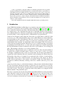
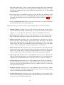
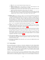
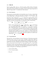
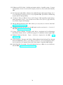
The display component can load such a file and display the different dimensions of the performance
space using three coupled tree browsers (Figure 1). The browsers are connected in such a way
that you can view one dimension with respect to another dimension. The connection is based on
selections: in each tree you can select one or more nodes. For example, in Figure 1 the Execution
4
metric, the sweep call path node, and Process 0 are selected. For each tree, the selections in the
trees on its left-hand-side (if any) restrict the considered data: The metric nodes aggregate data over
all call path nodes and all system items, the call tree aggregates data for the Execution metric
over all system nodes, and each node of the system tree shows the severity for the Execution metric
of the sweep call path node for this system node.
If the CUBE file contains topological information, the distribution of the performance metric across
the topology can be examined using the topology view. Furthermore, the display is augmented with
a source-code display that shows the position of a call site in the source code.
As performance tuning of parallel applications usually involves multiple experiments to compare
the effects of certain optimization strategies, CUBE includes a feature designed to simplify crossexperiment analysis. The CUBE algebra [7] is an extension of the framework for multi-execution
performance tuning by Karavanic and Miller [3] and offers a set of operators that can be used to
compare, integrate, and summarize multiple CUBE data sets. The algebra allows the combination of
multiple CUBE data sets into a single one that can be displayed and examined like the original ones.
In addition to the information provided by plain CUBE files a statistics file can be provided, enabling
the display of additional statistical information of severity values. Furthermore, a statistics file can
also contain information about the most severe instances of certain performance patterns – globally
as well as with respect to specific call paths. If a trace file of the program being analyzed is available,
the user can connect to a trace browser (i.e., Vampir or Paraver) and then use CUBE to zoom their
timelines to the most severe instances of the performance patterns for a more detailed examination
of the cause of these performance patterns.
The following sections explain how to use the CUBE display, how to create CUBE files, and how to
use the algebra and other tools.
2
Using the Display
This section explains how to use the CUBE QT display component. After installation, the executable
"cube3-qt" can be found in the specified directory of executables (specifiable by the “prefix”
argument of configure, see the CUBE Installation Manual). The program supports as an optional
command-line argument the name of a cube file that will be opened upon program start.
After a brief description of the basic principles, different components of the GUI will be described
in detail.
2.1
Basic Principles
The CUBE QT display has three tree browsers, each of them representing a dimension of the performance space (Figure 1). Per default, the left tree displays the metric dimension, the middle tree
displays the program dimension, and the right tree displays the system dimension. The nodes in
the metric tree represent metrics. The nodes in the program dimension can have different semantics
depending on the particular view that has been selected. In Figure 1, they represent call paths forming a call tree. The nodes in the system dimension represent machines, nodes, processes, or threads
from top to bottom.
Each node is associated with a value, which is called the severity and is displayed simultaneously
using a numerical value as well as a colored square. Colors enable the easy identification of nodes
5
Figure 1: CUBE display window.
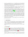
Figure 2: CUBE display window with expanded Execution metric node.
of interest even in a large tree, whereas the numerical values enable the precise comparison of
individual values. The sign of a value is visually distinguished by the relief of the colored square.
A raised relief indicates a positive sign, a sunken relief indicates a negative sign.
Users can perform two basic types of actions: selecting a node or expanding/collapsing a node. In
the metric tree on Figure 1, the metric Execution is selected. Selecting a node in a tree causes the
other trees on its right to display values for that selection. For the example of Figure 1, the metric
tree displays the total metric values over all call and system nodes, the call tree displays values for
the Execution metric over all system entities, and the system tree for the Execution metric and the
6
sweep call tree node. Briefly, a tree is always an aggregation over all selected nodes of its neighbor
trees to the left.
Collapsed nodes with a subtree that is not shown are marked by a [+] sign, expanded nodes with a
visible subtree by a [-] sign. You can expand/collapse a node by left-clicking on the corresponding
[+]/[-] signs. Collapsed nodes have inclusive values, i.e., their severity is the sum of the severities
over the whole collapsed subtree. For the example of Figure 1, the Execution metric value 1.23e7
is the total time for all executions. On the other hand, the displayed values of expanded nodes
are their exclusive values. E.g., the expanded Execution metric node in Figure 2 shows that the
program needed 3.18e6 seconds for execution other than MPI.
Note that expanding/collapsing a selected node causes the change of the current values in the trees
on its right-hand-side. As explained above, in our example in Figure 1 the call tree displays values
for the Execution metric over all system entities. Since the Execution node is collapsed, the
call tree severities are computed for the whole Execution metric’s subtree. When expanding the
selected Execution node, as shown in Figure 2, the call tree displays values for the Execution
metric without the MPI metric.
2.2
GUI Components
The GUI consists (from top to bottom) of
• a menu bar,
• a tool bar,
• three value mode combos,
• three resizable panes each containing some tabs,
• three selected value information widgets,
• a color legend, and
• a status bar.
The three resizable panes offer different views: the metric, the call, and the system pane. You
can switch between the different tabs of a pane by left-clicking on the desired tab at the top of the
pane. Note that the order of the panes can be changed (see the description of the menu item Display
⇒Dimension order in Section 2.2.1).
The metric pane contains a metric tree browser only. The call pane offers a call tree browser and a
flat call profile. The system pane has a metric tree browser, and possibly several topology views, if
corresponding topology data is defined in the CUBE file. Tree browsers also provide a context menu.
2.2.1
Menu Bar
The menu bar consists of three menus: a file menu, a display menu, and a help menu. Some menu
functions have also a keyboard shortcut, which is written beside the menu item’s name in the menu.
E.g., you can open a file with Ctrl+O without going into the menu. A short description of the menu
items is visible in the status bar if you stay for a short while with the mouse above a menu item.
7
1. File: The file menu offers the following functions:
(a) Open (Ctrl+O): Offers a selection dialog to open a CUBE file. In case of an already
opened file, it will be closed before a new file gets opened. If a file got opened successfully, it gets added to the top of the recent files list (see below). If it was already in the
list, it is moved to the top.
(b) Close (Ctrl+W): Closes the currently opened CUBE file. Disabled if no file is opened.
(c) Open external: Opens a file for the external percentage value mode (see Section 2.2.3).
(d) Close external: Closes the current external file and removes all corresponding data.
Disabled if no external file is opened.
(e) Connect to trace browser: This menu item is only visible if a CUBE file with a corresponding statistics file, containing information about the most severe instances of certain
performance patterns, is open (and CUBEwas configured for remote trace browsing). In
this case, it offers to connect to a trace browser (i.e., Vampir or Paraver) to examine
the behaviour of the program around the most severe pattern instances. For an in-depth
explanation of this feature see subsection 2.3.2.
(f) Settings: This menu item offers the saving, loading, and the deletion of settings. You
can save several settings under different names.
On the one hand, settings store the appearance of the application like the widget sizes,
color and precision settings, the order of panes, etc. On the other hand, settings can also
store which data is loaded, which tree nodes are expanded, etc. When saving a setting,
the appearance is always saved. While saving, you will be asked if you would also like
to save the data-related settings.
If you load a setting which stores also data settings, the corresponding data is also
loaded. In the dialog for loading settings you are offered the list of all available settings. For the settings with data we display after their name also the corresponding cube
file’s name in braces. Note that settings with data store only the cube file where to load
the data from, but not the data itself. Thus if the cube file is not available any more,
CUBE cannot load the data settings. CUBE also makes some basic tests on the data to
check if it could have changed since saving the setting. E.g., if the number of items does
not coincides with those upon saving, it also does not load the data.
(g) Dynamic loading threshold: By default, CUBE always loads the whole amount of data
when you open a CUBE file. However, CUBE offers also a possibility to load only those
data which is needed for the current display. To be more precise, the data for the selected
metric(s) and, if a selected metric is expanded, the data for its children are loaded. If
you change the metric selection, possibly some new data is needed for the display that
is dynamically loaded on demand. Currently not needed data gets unloaded.
This functionality is useful mostly for large files. Under this menu item you can define
a file size threshold (in bytes) above which CUBE offers you dynamic data loading. If a
file being opened is larger than this threshold, CUBE will ask you if you wish dynamic
loading.
(h) Screenshot: The function offers you to save a screenshot in a PNG file. Unfortunately
the outer frame of the main window is not saved, only the application itself.
(i) Quit (Ctrl+Q): Closes the application.
8
(j) Recent files: The last 5 opened files are offered for re-opening, the top-most being the
most recently opened one. A full path to the file is visible in the status bar if you move
the mouse above one of the recent file items in the menu.
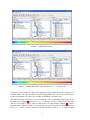
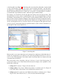
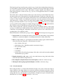
2. Display: The display menu offers the following functions:
(a) Dimension order: As explained above, CUBE has three resizable panes. Initially the
metric pane is on the left, the call pane is in the middle, and the system pane is on the
right-hand-side. However, sometimes you may be interested in other orders, and that is
what this menu item is about. It offers all possible pane orderings. For example, assume
you would like to see the metric and call values for a certain thread. In this case, you
should place the system pane on the left, the metric pane in the middle, and the call
pane on the right, as shown in Figure 3. Note that in panes left-hand-side of the metric
pane we have no meaningful values, since they miss a reference metric; in this case we
specify the values to be undefined, denoted by a “-” sign.
Figure 3: Modified pane order via the menu Display ⇒Dimension order.
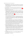
(b) General coloring: Opens a dialog where different color settings can be changed. The
dialog is show in Figure 4. The Ok button applies the settings to the display and closes
the dialog, the Apply button applies the settings to the display, and Cancel cancels
all changes since the dialog was opened (even if “Apply” was pressed in between) and
closes the dialog.
At the top of the dialog you see a color legend with some vertical black lines, showing
the position of the color scale start, the colors cyan, green, and yellow, and the color
scale end. These lines can be dragged with the left mouse button, or their position can
also be changed by typing in some values between 0.0 (left end) and 1.0 (right end)
below the color legend in the corresponding spins.
The different coloring methods offer different functions to interpolate the colors at positions between the above 5 data points.
9
Figure 4: The color dialog opened via the menu Display ⇒General coloring.
With the upper spin below the coloring methods you can define a threshold percentage
value between 0.0 and 100.0, below which colors are lightened. The nearer to the left
end of the color scale the stronger the lightening (with linear increase).
With the spin at the bottom of the dialog you can define a threshold percentage value
between 0.0 and 100.0, below which values should be colored white.
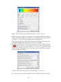
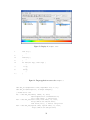
(c) Precision: Activating this menu item opens a dialog for precision settings (see Figure 5). Besides Ok and Cancel, the dialog offers an Apply button, that applies the
current dialog settings to the display. Pressing Cancel undoes all changes due to the
dialog, even if you already pressed Apply previously, and closes the dialog. Ok applies
the settings and closes the dialog.
Figure 5: The precision dialog opened via the menu Display ⇒Precision.
It consists of two parts: precision settings for the tree displays, and precision settings
10
Figure 6: The font dialog opened via the menu Display ⇒Trees ⇒Font.
for the selected value info widgets and the topology displays. For both formats, three
values can be defined:
i. Number of digits after the decimal point: As the name suggests, you can specify
the precision for the fraction part of the values. E.g., the number 1.234 is displayed
as 1.2 if you set this precision to 1, as 1.234 if you set it to 3, and as 1.2340 if you
set it to 4.
ii. Exponent representation above 10x with x: Here you can define above which
threshold we should use scientific notation. E.g., the value 1000 is displayed as
1000 if this value is larger then 3 and as 1e3 otherwise.
iii. Display zero values below 10−x with x: Due to inexact floating point representation it often happens that the users wish to round down values near by zero to zero.
Here you can define the threshold below which this rounding should take place.
E.g., the value 0.0001 is displayed as 0.0001 if this value is larger than 3 and as
zero otherwise.
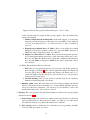
(d) Trees: This menu item offers two sub-items:
i. Font: Here you can specify the font, the font size (in pt), and the line spacing for
the tree displays (see Figure 6). The Ok button applies the settings to the display and
closes the dialog, the Apply button applies the settings to the display, and Cancel
cancels all changes since the dialog was opened (even if Apply was pressed in
between) and closes the dialog.
ii. Selection marking: Here you can specify if selected items in trees should be
marked by a blue background or by a frame.
(e) Optimize width: Under this menu item CUBE offers widget rescaling such that the
amount of information shown is maximized, i.e., CUBE optimally distributes the available space between its components. You can chose if you would like to stick to the
current main window size, or if you allow to resize it.
3. Topology: The topology menu offers the following functions related to the topology display
described in Section 2.2.5:
(a) Item coloring: Offers a choice how zero-valued system nodes should be colored in the
topology display. The two offered options are either to use white or to use white only if
all system leaf values are zero and use the minimal color otherwise.
(b) Line coloring: Allows to define the color of the lines in topology painting. Available
colors are black, gray, white, or no lines.
11
(c) Toolbar: This menu item allows to specify if the tool bar’s buttons should be labeled by
icons, by a text description, or if the tool bar should be hidden. For more information
about the tool bar see Section 2.2.2.
(d) Show also unused hardware in topology: if not checked, unused topology planes, i.e.,
planes whose grid elements don’t have any processes/threads assigned to, are hidden.
Unused plane elements, if not hidden, are colored gray.
(e) Topology antialiasing: if checked, antialiasing is used when painting lines in the
topologies.
4. Help: The help menu provides help on usage and gives some informations about CUBE.
(a) Getting started: Opens a dialog with some basic informations on the usage of CUBE.
(b) Mouse and keyboard control: Lists mouse and keyboard control as given in Section 2.4.
(c) What’s this?: Here you can get more specific information on parts of the CUBE GUI.
If you activate this menu item, you switch to the “What’s this?” mode. If you now click
on a widget an appropriate help text is shown. The mode is left when help is given or
when you press Esc.
Another way to ask the question is to move the focus to the relevant widget and press
Shift+F1.
(d) About: Opens a dialog with release information.
2.2.2
Tool bar
As already mentioned, the system pane may contain topology displays, if corresponding data is
specified in the CUBE file. For the topology displays see Section 2.2.5. Basically, a topology
display paints a two- or three-dimensional grid, in the form of some planes placed one above the
other. Each plane consists of a two-dimensional grid of processes or threads.
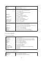
The tool bar is enabled only if the system pane shows a topology display, and it offers functions to
manipulate the display of the above grid planes. The tool bar can be labeled by icons, by text, or it
can be hidden, see menu Topology ⇒Toolbar in Section 2.2.1. The tool bar buttons have tool tips,
i.e., a short description pops up if the tool bar is enabled and you move the mouse above a button.
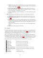
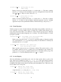
The functions are the following, listed from the left to the right in the topology tool bar:
Move left
Moves the whole topology to the left.
Move right
Moves the whole topology to the right.
Move up
Moves the whole topology upwards.
Move down
Moves the whole topology downwards.
Increase plane distance
Increase the distance between the planes of the topology.
Decrease plane distance
Decrease the distance between the planes of the topology.
Zoom in
Enlarge the topology.
Zoom out
Scale down the topology.
12
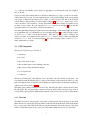
2.2.3
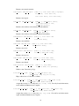
Reset
Reset the display. It scales the topology such that it fits
into the visible rectangle, and transforms it into a default
position.
Scale into window
It scales the topology such that it fits into the visible rectangle, without transformations.
Set minimum/maximum
values for coloring
Similarly to the functions offered in the context menu of
trees (see Section 2.2.4), you can activate and deactivate
the application of user-defined minimal and maximal values for the color extremes, i.e., the values corresponding
to the left and right end of the color legend. If you activate user-defined values for the color extremes, you are
asked to define two values that should correspond to the
minimal and to the maximal colors. All values outside of
this interval will get the color gray. Note that canceling
any of the input windows causes no changes in the coloring method. If user-defined min/max values are activated,
the selected value information widget displays a “(u)” for
“user-defined” behind the minimal and maximal color values.
x-rotation
Rotate the topology cube about the x-axis with the defined
angle.
y-rotation
Rotate the topology cube about the y-axis with the defined
angle.
Dimension order for
topology displays
The topologies may have two or three dimensions. Here
you can define the order of dimensions in the display.
Value modes
Each tree view has its own value mode combo, a drop-down menu above the tree, where it is possible
to change the way the severity values are displayed.
The default value mode is the Absolute value mode. In this mode, as explained below, the severity
values from the CUBE file are displayed. However, sometimes these values may be hard to interpret, and in such cases other value modes can be applied. Basically, there are three categories of
additional value modes.
• The first category presents all severities in the tree as percentage of a reference value. The
reference value can be the absolute value of a selected or a root node from the same tree or in
one of the trees on the left-hand-side. For example, in the Own root percent value mode the
severity values are presented as percentage of the own root’s (inclusive) severity value. This
way you can see how the severities are distributed within the tree. All the value modes 2–8
fall into this category.
All nodes of trees on the left-hand-side of the metric tree have undefined values. (Basically,
we could compute values for them, but it would sum up the severities over all metrics, that
have different meanings and usually even different units, and thus those values would not
13
have much expressiveness.) Since we cannot compute percentage values based on undefined
reference values, such value modes are not supported. For example, if the call tree is on the
left-hand-side, and the metric tree is in the middle, then the metric tree does not offer the Call
root percent mode.
• The second category is available for system trees only, and shows the distribution of the
values within hierarchy levels. E.g., the Peer percent value mode displays the severities as
percentage of the maximal value on the same hierarchy depth. The value modes 9–10 fall into
this category.
• Finally, the External percent value mode relates the severity values to severities from another
external CUBE file (see below for the explanation).
Depending on the type and position of the tree, the following value modes may be available:
1. Absolute (default): Available for all trees. The displayed values are the severity value as
read from the cube file, in units of measurement (e.g., seconds). Note that these values can be
negative, too, i.e., the expression “absolute” in not used in its mathematical sence here.
2. Own root percent: Available for all trees. The displayed node values are the percentage of
their absolute values with respect to the absolute value of their root node in collapsed state.
3. Metric root percent: Available for trees on the right-hand-side of the metric tree. The displayed node values are the percentage of their absolute values with respect to the absolute
value of the collapsed metric root node. If there are several metric roots, the root of the selected metric node is taken. Note, that multiple selection in the metric tree is possible within
one root’s subtree only, thus there is always a unique metric root for this mode.
4. Metric selection percent: Available for trees on the right-hand-side of the metric tree. The
displayed node values are the percentage of their absolute values with respect to the selected
metric node’s absolute value in its current collapsed/expanded state. In case of multiple selection, we take the sum of the selected metrics’ values for the percentage computation.
5. Call root percent: Available for trees on the right-hand-side of the call tree. Similar to the
metric root percent, but the call tree root instead of the metric tree root is considered. In case
of multiple selection with different call roots, the sum of those root values is considered.
6. Call selection percent: Available for trees on the right-hand-side of the call tree. Similarly to
the metric selection percent, percentage is computed with respect to the selected call node’s
value in its current collapsed/expanded state. In case of multiple selection we consider the
sum of the selected call values.
7. System root percent: Available for trees on the right-hand-side of the system tree. Similar
to the call root percent, where the sum of the inclusive values of all roots of selected system
nodes are considered for percentage computation.
8. System selection percent: Available for trees on the right-hand-side of the system tree. Similarly to the call selection percent, percentage is computed with respect to the selected system
node(s) in its current collapsed/expanded state.
14
9. Peer percent: For the system tree only. The peer percentage mode shows the percentage of
the nodes’ inclusive absolute values relative to the largest inclusive absolute peer value, i.e.,
to the largest inclusive value between all entities on the current hierarchy depth. For example,
if there are 3 threads with inclusive absolute values 100, 120, and 200, then they have the peer
percent values 50,60, and 100.
10. Peer distribution: For the system tree only. The peer distribution mode shows the percentage
of the system nodes’ inclusive absolute values on the scale between the minimum and the
maximum of peer inclusive absolute values. For example, if there are 3 threads with absolute
values 100, 120, and 200, then they have the peer distribution values 0, 20, and 100.
11. External percent: Available for all trees, if the metric tree is the left-most widget. To facilitate the comparison of different experiments, users can choose the external percentage mode
to display percentages relative to another data set. The external percentage mode is basically
like the metric root percentage mode except that the value equal to 100% is determined by
another data set.
In all modes, the severity values for expanded system nodes are shown as undefined, denoted by a
“-” sign. The reason is, that such nodes do not execute. Only leaf system nodes can have non-zero
exclusive values, but they are not expandable.
2.2.4
Tree browsers
A tree browser displays different hierarchical data structures in form of trees. Currently supported
tree types are metric tree, call tree, call flat profile, and system tree. The structure of the displayed
data is common in all trees: The indentation of the tree nodes reflects the hierarchical structure.
Expandable nodes, i.e., nodes with non-hidden children, are equipped with a [+]/[-] sign ([+] for
collapsed and [-] for expanded nodes). Furthermore, all nodes have a color icon, a value, and a
label.
The value of a node is computed, as explained earlier, basing on the current selections in the lefthand-side trees and on the current value mode. The precision of the value display in trees can
be modified, see the menu item Display ⇒Precision in Section 2.2.1. The color icon reflects the
position of the node’s value between 0.0 and a maximal value. These maximal value is the maximal
value in the tree for the absolute value mode, and 100.0 else. See the menu item Display ⇒General
coloring in Section 2.2.1 and the context menu item Min/max values in the context menu description
below for color settings.
A label in the metric tree shows the metric’s name. A label in the call tree shows the last callee
of a particular call path. If you want to know the complete call path, you must read all labels
from the root down to the particular node you are interested in. After switching to the flat profile
view (see below), labels in the flat call profile denote methods or program regions. A label in the
system tree shows the name of the system resource it represents, such as a node name or a machine
name. Processes and threads are usually identified by a rank number, but it is possible to give
them specific names when creating a CUBE file. The thread level of single-threaded applications is
hidden. Multiple root nodes are supported.
After opening a data set the middle panel shows the call tree of the program. However, a user
might wish to know which fraction of a metric can be attributed to a particular region (e.g., method)
regardless of from where it was called. In this case, you can switch from the call-tree view (default)
15
to the flat-profile view (Figure 7). In the flat-profile view, the call-tree hierarchy is replaced with
a source-code hierarchy consisting of two levels: regions and their subroutines. Any subroutines
are displayed as a single child node labeled Subroutines. A subroutine node represents all regions
directly called from the region above. In this way, you are able to see which fraction of a metric is
associated with a region exclusively, that is, without its regions called from there.
Tree displays are controlled by the left and right mouse buttons and some keyboard keys. The
left mouse button is used to select or expand/collapse a node: You can expand/collapse a node by
left-clicking on the attached [+]/[-] sign, and select it by left-clicking elsewhere in the node’s line.
Please use Ctrl + left mouse button for multiple selection/deselection. Selection without the Ctrl key
deselects all previously selected nodes and selects the clicked node. In single selection mode you
can also use the up/down arrows to move the selection one node up/down. The right mouse button
is used to pop up a context menu with node-specific information, such as online documentation (see
the description of the context menu below).
Figure 7: CUBE flat profile.
Each tree has its own context menu, that can be activated by a right-mouse-click within the tree’s
window. If you right-click on one of the tree’s nodes, this node gets framed, and serves as a reference
node for some of the menu items. If you click outside of tree items, there is no refernce node, and
some menu items are disabled.
The context menu consists, depending on the type of the tree, of some of the following items. If
you move the mouse over a context menu item, the status bar displays some explanation of the
functionality of that item.
1. Collapse all: For all trees. Collapses all nodes in the tree.
2. Collapse subtree: For all trees. Enabled only if there is a reference node. It collapses all
nodes in the subtree of the reference node (inclusively the reference node).
3. Collapse peers: For system trees only. Enabled only if there is a reference node. Collapses
all peer nodes of the reference node, i.e., all nodes at the same hierarchy depth.
16
4. Expand all: For all trees. Expands all nodes in the tree.
5. Expand subtree: For all trees. Enabled only if there is a reference node. Expands all nodes
in the subtree of the reference node (inclusively the reference node).
6. Expand peers: For system trees only. Enabled only if there is a reference node. Expands all
peer nodes of the reference node, i.e., all nodes at the same hierarchy depth.
7. Expand largest: For all trees. Enabled only if there is a reference node. Starting at the reference node, expands its child with the largest inclusive value (if any), and continues recursively
with that child until it finds a leaf. It is recommended to collapse all nodes before using this
function in order to be able to see the path along the largest values.
8. Dynamic hiding: Not available for metric trees. This menu item activates dynamic hiding.
All currently hidden nodes get shown. You are asked to define a percentage threshold between
0.0 and 100.0. All nodes whose color position on the color scale (in percent) is below this
threshold get hidden. As default value, the color percentage position of the reference node is
suggested, if you right-clicked over a node. If not, the default value is the last threshold. The
hiding is called dynamic, because upon value changes (caused for example by changing the
node selection) hiding is re-computed for the new values. With other words, value changes
may change the visibility of the nodes.
(a) Redefine threshold: This menu item is enabled if dynamic hiding is already activated.
This function allows to re-define the dynamic hiding threshold as described above.
During dynamic hiding, for expanded nodes with some hidden children and for nodes with
all of its children hidden, their displayed (exclusive) value includes the hidden children’s
inclusive value. After this sum we display in brackets the percentage of the hidden children’s
value in it.
9. Static hiding: Not available for metric trees. This menu item activates static hiding. All
currently hidden nodes keep being hidden. Additionally, you can hide and show nodes using
the now enabled sub-items:
(a) Static hiding of minor values: Enabled only in the static hiding mode. As described
under dynamic hiding, you are asked for a hiding threshold. All nodes whose current
color position on the color scale is below this percentage threshold get hidden. However,
in contrast to dynamic hiding, these hidings are static: Even if after some value changes
the color position of a hidden node gets above the threshold, the node keeps being
hidden.
(b) Hide this: Enabled only in the static hiding mode if there is a reference node. Hides the
reference node.
(c) Show children of this: Enabled only in the static hiding mode if there is a reference
node. Shows all hidden children of the reference node, if any.
Like for dynamic hiding, for expanded nodes with some hidden children and for nodes with
all of its children hidden, their displayed (exclusive) value includes the hidden children’s
inclusive value. After this sum we display in brackets the percentage of the hidden children’s
value in it.
17
10. No hiding: Not available for metric trees. This menu item deactivates any hiding, and shows
all hidden nodes.
11. Find items: For all trees. Opens a dialog to get a regular expression from the user. If the
user called the context menu over an item, the default text is the name of the reference node,
otherwise it is the last regular expression which was searched for.
The function marks by a yellow background all non-hidden nodes whose names contain the
given text, and by a light yellow background all collapsed nodes whose subtree contains such
a non-hidden node. The current found node, that is initialized to the first found node, is
marked by a distinguishable yellow hue.
12. Find next: For all trees. Changes the current found node to the next found node. If you did
not start a search yet, then you are asked for the regular expression to search for.
13. Clear found items: For all trees. Removes the background markings of the preceding find
items.
14. Info: For all trees (for call trees under Called region). Gives some short information about
the reference node. Disabled if there is no reference node or if no information is available for
the reference node.
15. Online description: For metric trees and flat call profiles (for call trees see under Called
region). Shows some (usually more extensive) online description for the reference node. For
example, metrics might point to an online documentation explaining their semantics, or regions representing library functions might point to the corresponding library documentation.
Disabled if there is no reference node or if no online information is available.
16. Location: For flat profiles only. Disabled if there is no reference node. Displays information
about the module and position within the module (line numbers) where the method is defined.
17. Source code: For flat call profiles only (for call trees see Call site and Called region below).
Disabled if there is no reference node. Opens an editor for displaying, editing, and saving the
source code of the method/region for which the reference node stays for. The begin and the
end of the method/region are highlighted. If the specified source file is not found, you are
asked to chose a file to open.
The file is in a read only mode per default. If you wish to edit the text, please uncheck the
Read only box in the bottom left corner. For keyboard and mouse control see Section 2.4.2.
18. Call site: For call trees only. Enabled only if there is a reference node. Offers information
about the caller of the reference node.
(a) Location: Displays information about the module and position within the module (line
numbers) of the caller of the reference node.
(b) Source code: Opens an editor for displaying, editing, and saving the source code where
the call for which the reference node stays for happens. The begin and the end of the
relevant source code region are highlighted. If the specified source file is not found, you
are asked to chose a file to open.
19. Called region: For call trees only. Enabled only if there is a reference node. Offers information about the reference node.
18
(a) Info: Gives some short information about the reference node.
(b) Online description: Shows some (usually more extensive) online description for the
reference node. Disabled if no online description is available.
(c) Location: Displays information about the module and position within the module (line
numbers) where the callee method of the reference node is defined.
(d) Source code: Opens an editor for displaying, editing, and saving the source code of the
callee of the reference node. Begin and end of the relevant region are highlighted. If the
specified source code does not exists, you are asked to chose a file to open.
20. Min/max values: Not for metric trees. Here you can activate and deactivate the application
of user-defined minimal and maximal values for the color extremes, i.e., the values corresponding to the left and right end of the color legend. If you activate user-defined values for
the color extremes, you are asked to define two values that should correspond to the minimal
and to the maximal colors. All values outside of this interval will get the color gray. Note that
canceling any of the input windows causes no changes in the coloring method. If user-defined
min/max values are activated, the selected value information widget (see Section 2.2.6) displays a “(u)” for “user-defined” behind the minimal and maximal color values.
21. Statistics: Only available if a statistics file for the current CUBE file is provided. Displays
statistical information about the instances of the selected metric in the form of a box plot. For
an in-depth explanation of this feature see subsection 2.3.1.
22. Max severity in trace browser: Only available for metric and call trees and only if a statistics
file providing information about the most severe instance(s) of the selected metric is present.
If CUBE is already connected to a trace browser (via File ⇒Connect to trace browser), the
timeline display of the trace browser is zoomed to the position of the occurrence of the most
severe pattern so that the cause for the pattern can be examined further. For a more detailed
explanation of this feature see subsection 2.3.2.
23. Sort by value (descending): For flat call profiles only. Sorts the nodes by their current values
in descending order. Note that if an item is expanded, its exclusive value is taken for sorting,
otherwise its inclusive value.
24. Sort by name (ascending): For flat call profiles only. Sorts the nodes alphabetically by name
in ascending order.
2.2.5
Topology Display
In many parallel applications, each process (or thread) communicates only with a limited number
of processes. The parallel algorithm divides the application domain into smaller chunks known as
sub-domains. A process usually communicates with processes owning sub-domains adjacent to its
own. The mapping of data onto processes and the neighborhood relationship resulting from this
mapping is called virtual topology. Many applications use one or more virtual topologies specified
as one-, two- or three-dimensional Cartesian grids.
Another sort of topologies are physical topologies reflecting the hardware structure on which the
application was run. A typical three-dimensional physical topology is given by the (hardware) nodes
in the first dimension, and the arrangement of cores/processors on nodes in further two dimensions.
19
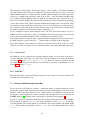
The CUBE display supports one-, two-, and three-dimensional Cartesian grids. If the currently
opened cube file defines such a topology, the topology display shows performance data mapped
onto the Cartesian topology of the application. The corresponding grid is specified by the number
of dimensions and the size of each dimension. Threads/processes are attached to the grid elements,
as specified by the CUBE file. Not all system items have to be attached to a grid element, and not
every grid element has a system item attached. Examples of a two- and of a three-dimensional
topology are shown on Figure 8. Note that the topology tool bar is enabled when a topology is
displayed.
Figure 8: Topology Display
20
The Cartesian grid is presented by planes stacked on top of each other in a three dimensional projection. The number of planes depends on the number of dimensions in the grid. Each plane is divided
into squares (typically shown as rombi). The number of squares depends on the dimension size.
Each square represents a system resource (e.g., a process) of the application and has a coordinate
associated with it.
The current value of each grid element (with respect to the selections on the left-hand-side and to
the current value mode) is represented by coloring the grid element. To make use of the whole color
scale, coloring in topologies in the absolute value mode is based on the minimal and the maximal
system leaf values, instead of considering all system items, as for the system tree coloring. In all
other value modes, coloring is based on a value scale from 0.0 to 100.0. Grid elements without
having a system item attached to it are colored gray. See Section 2.2.1 (menu Topology) for further
topology-specific coloring settings. For example, the upper topology in Figure 8 is painted without
lines, and the one below with black lines and topology line antialiasing.
If the selected system item (or the first selected one in case of multiple selection) occurs in the
topology, it is marked by an additional frame and by additional lines at the side of the plane which
contains the corresponding grid, such that the selected item’s position is also visible if the corresponding plane is not completely visible.
Besides the functions offered by the topology tool bar (see 2.2.2), the following issues are supported:
1. Item selection: You can change the current system selection by left-clicking on a grid element
which has a system item assigned to it (resulting in the selection of that system item).
2. Info: By right-clicking on a grid element an information widget appears with information
about the system item assigned to it. The information contains
• the coordinate of the grid,
• the hardware node to which the attached system item belongs to,
• the system item’s name,
• its MPI rank,
• its identifier,
• and its value, followed by the percentage of this value on the scale between the minimal
and maximal topology values.
3. Rotation about the x and y axes: can be done with left-mouse drag (click and hold the
left-mouse button while moving the mouse).
4. Increasing/decreasing the distance between the planes: with Ctrl+<left-mouse drag>
5. Moving the whole topology up/down/left/right: with Shift+<left-mouse drag>
2.2.6
Selected value info
Below each pane there is a selected value information widget. If no data is loaded, the widget is
empty. Otherwise, the widget displays more extensive and precise information about the selected
values in the tree above. This information widget and the topologies may have different precision
settings than the trees, such that there is the possibility to display more precise information here
than in the trees (see Section 2.2.1, menu Display ⇒Precision).
21
The widget has a 3-line display. The first line displays at most 4 numbers. The left-most number
shows the smallest value in the tree (or 0.0 in any percentage value mode for trees, or the userdefined minimal value for coloring if activated), and the right-most number shows the largest value
in the tree (or 100.0 in any percentage value mode in trees, or the user-defined maximal value
for coloring if activated). Between these two numbers the current value of the selected node is displayed, if it is defined. Additionally, in the absolute value mode it follows in brackets the percentage
of the selected value on the scale between the minimal and maximal values. Note that the values
of expanded non-leaf system nodes and of nodes of trees on the left-hand-side of the metric tree
are not defined. If the value mode is not the absolute value mode, then in the second line similar
information is displayed for the absolute values in a light gray color.
In case of multiple selection, the information refers to the sum of all selected values. In case of
multiple selection in system trees in the peer distribution and in the peer percent modes this sum
does not state any valuable information, but it is displayed for consistency reasons.
If the widget width is not large enough to display all numbers in the given precision, then a part of
the number displays get cut down and a “. . .” indicates that not all digits could be displayed.
Below these numbers, in the third line a small color bar shows the position of the color of the
selected node in the color legend. In case of undefined values, the legend is filled with a gray grid.
2.2.7
Color Legend
By default, the colors are taken from a spectrum ranging from blue over cyan, green, and yellow to
red, representing the whole range of possible values. You can change the color settings in the menu,
see Section 2.2.1, menu Display ⇒General coloring. Exact zero values are represented by the
color white (in topologies you can decide if you would like to use white or the minimal color, see
Section 2.2.1, menu Topology).
2.2.8
Status Bar
The status bar displays some status information, like state of execution for longer procedures, hints
for menus the mouse pointing at etc.
2.3
Features enabled through statistic files
In this section we will explain two features – namely the display of statistical information about
performance patterns which represent performance problems and the display of the most severe
instances of these patterns in a trace browser – which both are only available if a statistic file for
the currently opened CUBE file is present. Currently, such a statistic file can be generated by the
EXPERT analyzer [9]. The file format of statistic files is described in the appendix A.
In order for CUBE to recognize the statistic file it must be placed in the same folder as the CUBE file.
If the CUBE file is named expert.cube, the statistic file must be called epik.stat. In any other
case the basename of the statistic file has to be identical to that of the CUBE file, but with the suffix
.stat. If for example the CUBE file is called foo.cube, the corresponding statistic file is called
foo.stat
22
2.3.1
Statistical information about performance patterns
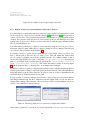
If a statistic file is provided, you can view statistical information about one or multiple patterns (for
example in order to compare them). This is done by selecting the desired metrics in the metric tree
and then selecting the Statistics menu item in the context menu. This brings up the box plot window
as shown in figure 9.
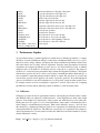
The box plot shows a graphical representation of the statistical data of the selected patterns. The
slender black lines on the top and the bottom designate the maximum and the minimum measured
severity of the pattern, respectively. The lower and the upper borders of the white box indicate the
values of the 25% and 75% quantile. The thick line inside the box represents the median of the
values while the dashed line indicates the mean.
There are two ways of interacting with the box plot. You can zoom to a certain interval on the
y-axis by clicking on a position with the height of the desired maximal or minimal value and by
consecutively dragging the mouse to a position with the height of the corresponding other extreme
value. You can reset the view (that is to undo all zooming) by clicking the middle mouse button
somewhere on the box plot.
If you are interested in more precise values for the severity statistics of a certain metric, you can
click somewhere in the column of the desired metric, which will yield a small window (as shown in
the top right corner of figure 9) displaying the exact values of the statistics.
Figure 9: Screenshot of a box plot as shown by CUBE displaying statistical information about the
selected patterns. The additional window on the top right displaying the exact values of the statistics.
23
[D-BUS Service]
Name=com.gwt.vampir
Exec=/private/utils/bin/vng+
Figure 10: An example of the com.gwt.vampir.service file
2.3.2
Display of most severe pattern instances using a trace browser
If a statistic file also contains information about the most severe instances of certain patterns, CUBE
can be connected to a trace browser (currently Vampir [2, 8] and Paraver [4, 1] are supported) in
order to view the state of the program being analyzed at the time this most severe pattern instance
occurred. For collective operations, the most severe instance is the one with the largest sum of the
waiting times of all processes, which is not necessarily the one with the largest maximal waiting
time of each individual process.
To use this feature you first have to connect to a trace browser by using the Connect to trace browser
menu item of the File menu, which offers to connect to Vampir as well as to Paraver. This will open
one of the two dialog windows shown in figure 11.
For Vampir you have to specify the host name and port of the Vampir server you want to connect to and the path of the trace file you want to load. This will launch the Vampir client
(if it is correctly configured) and load the specified trace file. To configure Vampir so that it
can be started automatically by CUBE, a service file (com.gwt.vampir.service), describing the
path to your Vampir client executable must be placed under /usr/share/dbus-1/service or
$HOME/.local/share/dbus-1/services. This service file must be exactly as shown in figure
10 with the exception that Exec should point to your Vampir client executable.
For Paraver, you have to specify a configuration file (which is used to initialize the Paraver window
which is opened when zooming) as well as the path of the desired trace file. This will launch Paraver
which will directly open the correct trace file. In order for CUBE to be able to launch Paraver, the
executable directory of Paraver must be in your path.
It is also possible to connect to multiple trace browsers so that you can view a trace file in Paraver
and Vampir simultaneously, but due to limitations with the Vampir client you can only have two
Vampir clients running at the same time. All trace browsers will be zoomed simultaneously if you
select a zoom command (as described below).
Figure 11: The dialog windows for a connection to Vampir and to Paraver.
Once CUBE is connected to a trace browser you can select the Max severity in trace browser menu
24
item of the metric tree so that all connected trace browsers are zoomed to the (globally) most severe
instance of the selected pattern.
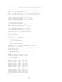
A more sophisticated feature is the ability to zoom to the most severe instance of a pattern in a
selected call path. This can be done by selecting a metric in the metric tree which will highlight the
most severe call paths in the call tree. You can then use the context menu of the call tree to select the
Max severity in trace browser menu item (see figure 12 for illustration). This menu item will then
zoom all connected trace browsers to the most severe instance of the selected pattern with respect
to the chosen call path.
Figure 12: CUBE display window with a selected metric and a context menu called on the same
metric in a special call path, showing the Max severity in trace browser menu item.
2.4
2.4.1
Keyboard and mouse control
General control
Shift+F1
Help: What’s this?
25
Ctrl+O
Ctrl+W
Ctrl+Q
Left click
Right click
Ctrl+Left click
Left drag
Ctrl+Left drag
Shift+Left drag
Mouse wheel
Up arrow
Down arrow
Left arrow
Right arrow
Page up
Page down
2.4.2
Shortcut for menu File ⇒Open
Shortcut for menu File ⇒Close
Shortcut for menu File ⇒Quit
over menu/tool bar: activate menu/function
over value mode combo: select value mode
over tab: switch to tab
in tree: select/deselect/expand/collapse items
in topology: select item
in tree: context menu
in topology: context information
in tree: multiple selection/deselection
over scroll bar: scroll
in topology: rotate topology
in topology: increase plane distance
in topology: move topology
in topology: zoom in/out
in tree: move selection one item up (single-selection only)
in topology/scroll area: scroll one unit up
in tree: move selection one item down (single-selection only)
in topology/scroll area: scroll one unit down
in scroll area: scroll to the left
in scroll area: scroll to the right
in tree/topology/scroll area: scroll one page up
in tree/topology/scroll area: scroll one page down
Source code editor
Control in read only mode:
Up Arrow
Down Arrow
Left Arrow
Right Arrow
Page Up
PageDown
Home
End
Mouse wheel
Alt+Mouse wheel
Ctrl+Mouse wheel
Ctrl+A
Move one line up
Move one line down
Scroll one character to the left (if horizontally scrollable)
Scroll one character to the right (if horizontally scrollable)
Move one (viewport) page up
Move one (viewport) page down
Move to the beginning of the text
Move to the end of the text
Scroll the page vertically
Scroll the page horizontally (if horizontally scrollable)
Zoom the text
Select all text
Additionally for the read and write mode:
Left Arrow
Right Arrow
Backspace
Move one character to the left
Move one character to the right
Delete the character to the left of the cursor
26
Delete
Ctrl+C
Ctrl+Insert
Ctrl+K
Ctrl+V
Shift+Insert
Ctrl+X
Shift+Delete
Ctrl+Z
Ctrl+Y
Ctrl+Left arrow
Ctrl+Right arrow
Ctrl+Home
Ctrl+End
Hold Shift + some movement (e.g., Right arrow)
3
Delete the character to the right of the cursor
Copy the selected text to the clipboard
Copy the selected text to the clipboard
Delete to the end of the line
Paste the clipboard text into text edit
Paste the clipboard text into text edit
Delete the selected text and copy it to the clipboard
Delete the selected text and copy it to the clipboard
Undo the last operation
Redo the last operation
Move the cursor one word to the left
Move the cursor one word to the right
Move the cursor to the beginning of the text
Move the cursor to the end of the text
Select region
Performance Algebra
As performance tuning of parallel applications usually involves multiple experiments to compare
the effects of certain optimization strategies, CUBE offers a mechanism called performance algebra
that can be used to merge, subtract, and average the data from different experiments and and view
the results in the form of a single “derived” experiment. Using the same representation for derived
experiments and original experiments provides access to the derived behavior based on familiar
metaphors and tools in addition to an arbitrary and easy composition of operations. The algebra is
an ideal tool to verify and locate performance improvements and degradations likewise. The algebra
includes three operators diff, merge, and mean provided as command-line utilities which take two or
more CUBE files as input and generate another CUBE file as output. The operations are closed in the
sense that the operators can be applied to the results of previous operations. Note that although all
operators are defined for any valid CUBE data sets, not all possible operations make actually sense.
For example, whereas it can be very helpful to compare two versions of the same code, computing
the difference between entirely different programs is unlikely to yield any useful results.
3.1
Difference
Changing a program can alter its performance behavior. Altering the performance behavior means
that different results are achieved for different metrics. Some might increase while others might
decrease. Some might rise in certain parts of the program only, while they drop off in other parts.
Finding the reason for a gain or loss in overall performance often requires considering the performance change as a multidimensional structure. With CUBEś difference operator, a user can view
this structure by computing the difference between two experiments and rendering the derived result experiment like an original one. The difference operator takes two experiments and computes a
derived experiment whose severity function reflects the difference between the minuend’s severity
and the subtrahend’s severity.
Usage: cube3 diff [-o output] [-c] [-C] [-h] minuend subtrahend
27
-o Name of the output file (default: diff.cube)
-c Do not collapse system dimension, if experiments are incompatible
-C Collapse system dimension!
-h Help; Output a brief help message.
3.2
Merge
The merge operator’s purpose is the integration of performance data from different sources. Often a
certain combination of performance metrics cannot be measured during a single run. For example,
certain combinations of hardware events cannot be counted simultaneously due to hardware resource
limits. Or the combination of performance metrics requires using different monitoring tools that
cannot be deployed during the same run. The merge operator takes an arbitrary number of CUBE
experiments with a different or overlapping set of metrics and yields a derived CUBE experiment
with a joint set of metrics.
Usage: cube3 merge [-o output] [-c] [-C] [-h] cube ...
-o Name of the output file (default: merge.cube)
-c Do not collapse system dimension, if experiments are incompatible
-C Collapse system dimension!
-h Help; Output a brief help message.
3.3
Mean
The mean operator is intended to smooth the effects of random errors introduced by unrelated system
activity during an experiment or to summarize across a range of execution parameters. You can
conduct several experiments and create a single average experiment from the whole series. The
mean operator takes an arbitrary number of arguments.
Usage: cube3 mean [-o output] [-c] [-C] [-h] cube ...
-o Name of the output file (default: mean.cube)
-c Do not collapse system dimension, if experiments are incompatible
-C Collapse system dimension!
-h Help; Output a brief help message.
4
Creating CUBE Files
The CUBE data format in an XML instance [10]. The CUBE library provides an interface to create
CUBE files. It is a simple class interface and includes only a few methods. This section first describes
the CUBE API and then presents a simple C++ program as an example of how to use it.
28
4.1
CUBE API
The class interface defines a class Cube. The class provides a default constructor and fourteen
methods. The methods are divided into four groups. The first three groups are used to define the
three dimensions of the performance space and the last group is used to enter the actual data. In
addition, an output operator << to write the data to a file is provided.
4.1.1
Metric Dimension
This group refers to the metric dimension of the performance space. It consists of a single method
used to build metric trees. Each node in the metric tree represents a performance metric. Metrics have different units of measurement. The unit can be either “sec” (i.e., seconds) for time
based metrics, such as execution time, or “occ” (i.e., occurrences) for event-based metrics, such as
floating-point operations. During the establishment of a metric tree, a child metric is usually more
specific than its parent, and both of them have same unit of measurement. Thus, a child performance
metric has to be a subset of its parent metric (e.g., system time is a subset of execution time).
Metric* def met
(string disp name, string uniq name,
string dtype, string uom, string val, string url,
string descr, Metric* parent);
Returns a metric with display name disp name, unique name uniq name and description
descr. dtype specifies the data type, which can either be “INTEGER” or “FLOAT”. uom is the
unit of measurement, which is either “sec” for seconds or “occ” for number of occurrences.
The val field specifies if there is any data available for this particular metric. It can either
be “VOID” (no data available, metric will not be shown in CUBE) or an empty string (metric
will be shown and data is present). parent is a previously created metric which will be the
new metric’s parent. To define a root node, use NULL instead. url is a link to an HTML page
describing the new metric in detail. If you want to mirror the page at several locations, you
can use the macro @mirror@ as a prefix, which will be replaced by an available mirror
defined using def mirror() (see Section 4.1.6).
4.1.2
Program Dimension
This group refers to the program dimension of the performance space. The entities presented in this
dimension are region, call site, and call-tree node (i.e., call paths). A region can be a function, a
loop, or a basic block. Each region can have multiple call sites from which the control flow of the
program enters a new region. Although we use the term call site here, any place that causes the program to enter a new region can be represented as a call site, including loop entries. Correspondingly,
the region entered from a call site is called callee, which might as well be a loop. Every call-tree
node points to a call site. The actual call path represented by a call-tree node can be derived by
following all the call sites starting at the root node and ending at the particular node of interest. You
can choose among three ways of defining the program dimension:
1. Call tree with line numbers
2. Call tree without line numbers
3. Flat profile
29
A call tree with line numbers is defined as a tree whose nodes point to call sites. A call tree without
line numbers is defined as a tree whose nodes point to regions (i.e., the callees). A flat profile is
simply defined as a set of regions, that is, no tree has to be defined.
Region* def region
(string name, long begln, long endln,
string url, string descr,
string mod);
Returns a new region with region name name and description descr. The region is located
in the module mod and exists from line begln to line endln. url is a link to an HTML page
describing the new region in detail. For example, if the region is a library function, the url
can point its documentation. If you want to mirror the page at several locations, you can use
the macro @mirror@ as a prefix, which will be replaced by an available mirror defined using
def mirror() (see Section 4.1.6).
Cnode* def cnode
(Region* callee,
string mod, int line,
Cnode* parent);
Returns a new call-tree node representing a call from call site located at the line line of the
module mod. The call tree node calls the callee callee (i.e., a previously defined region).
parent is a previously created call-tree node which will be the new one’s parent. To define a
root node, use NULL instead. This method is used to create a call tree with line numbers.
Cnode* def cnode
(Region* region,
Cnode* parent);
Defines a new call-tree node representing a call to the region region. parent is a previously
created call-tree node which will be the new one’s parent. To define a root node, use NULL
instead. Note that different from the previous def cnode(), this method is used to create a
call-tree without line numbers where each call-tree node points to a region.
To define a call tree with line numbers use def cnode(Region*, string, int...). To define a
call tree without line numbers use def cnode(Region*, Cnode*) instead. To create a flat profile
use neither one — just defining a set of regions will be sufficient.
4.1.3
System Dimension
This group refers to the system dimension of the performance space. It reflects the system resources
which the program is using at runtime. The entities present in this dimension are machine, node,
process, and thread, which populate four levels of the system hierarchy in the given order. That
is, the first level consists of machines, the second level of nodes, and so on. Finally, the last (i.e.,
leaf) level is populated only by threads. The system tree is built in a top-down way starting with a
machine. Note that even if every process has only one thread, users still need to define the thread
level.
Machine* def mach
(string name);
Returns a new machine with the name name.
Node* def node
(string name, Machine* mach);
Returns a new (SMP) node which has the name name and which belongs to the machine mach.
30
Process* def proc
(string name, int rank,
Node* node);
Returns a new process which has the name name and the rank rank. The rank is a number
from 0 − (n − 1), where n is the total number of processes. MPI applications may use the rank
in MPI COMM WORLD. The process runs on the node node.
Thread* def thrd
(string name, int rank,
Process* proc);
Defines a new thread which has the name name and the rank rank. The rank is a number
from 0 − (n − 1), where n is the total number of threads spawned by a process. OpenMP
applications may use the OpenMP thread number. The thread belongs to the process proc.
4.1.4
Virtual Topologies
Virtual topologies are used to describe adjacency relationships among machines, SMP nodes, processes or threads. A topology usually consists of a single class of entities such as threads or processes. The CUBE API provides a set of functions to create Cartesian topologies and to define the
machine/SMP node/process/thread mappings onto coordinates. Note that the definition of virtual
topologies is optional.
Cartesian* def cart
(long ndims, const vector<long>& dimv,
const vector<bool>& periodv);
Defines a new Cartesian topology. ndims and dimv specify the number of dimensions and the
size of each dimension. periodv specifies the periodicity for each dimension. Currently, the
maximum value for ndims is three.
void def coords
(Cartesian* cart, Sysres* sys,
const vector<long>& coordv);
Maps a specific system resource onto a Cartesian coordinate. The system resource sys may
be a machine, SMP node, process or a thread. It is not recommended to map a mixed set of
entities onto one topology (e.g., machines and threads are located in the same topology). The
parameter of cart has been defined by the above def cart() method.
4.1.5
Severity Mapping
After the establishment of performance space, users can assign severity values to points of the
space. Each point is identified by a tuple (met, cnode, thrd). The value should be inclusive
with respect to the metric, but exclusive with respect to the call-tree node, that is it should not cover
its children. The default severity value for the data points left undefined is zero. Thus, users only
need to define non-zero data points.
void set sev
(Metric* met, Cnode* cnode,
Thread* thrd, double value);
Assigns the value value to the point (met, cnode, thrd).
void add sev
(Metric* met, Cnode* cnode,
Thread* thrd, double value);
31
Adds the value value to the present value at point (met, cnode, thrd).
The previous two methods set sev() and add sev() are intended to be used when the program
dimension contains a call tree and not a flat profile. As the flat profile does not require the definition
of call-tree nodes, the following two functions should be used instead:
void set sev
(Metric* met, Region* region,
Thread* thrd, double value);
Assigns the value value to the point (met, region, thrd).
void add sev
(Metric* met, Region* region,
Thread* thrd, double value);
Adds the value value to the present value at point (met, region, thrd).
4.1.6
Miscellaneous
Often users may want to define some information related to the CUBE file itself, such as the creation
date, experiment platform, and so on. For this purpose, CUBE allows the definition of arbitrary
attributes in every CUBE data set. An attribute is simply a key-value pair and can be defined using
the following method:
void def attr
(string key, string value);
Assigns the value value to the attribute key.
allows using multiple mirrors for the online documentation associated with metrics and regions. The url expression supplied as an argument for def metric() and def region() can
contain a prefix @mirror@. When the online documentation is accessed, CUBE can substitute all
mirrors defined for the prefix until a valid one has been found. If no valid online mirror can be
found, CUBE will substitute the ./doc directory of the installation path for @mirror@.
CUBE
void def mirror
(string mirror);
Defines the mirror mirror as potential substitution for the URL prefix @mirror@.
4.1.7
Writer Library in C
In order to create data files, another possibility is to use the C version of the CUBE writer API. The
interface defines a struct cube t and provides the following functions:
cube t* cube create();
Returns a new CUBE structure.
void cube free(cube t* c);
Destroys the given CUBE structure.
cube metric* cube def met
(cube t* c, const char*
const char* uniq name,
const char* uom, const
const char* url, const
cube metric* parent);
32
disp name,
const char* dtype,
char* val,
char* descr,
Returns a new metric structure.
cube region* cube def region
(cube t* c, const char* name, long begln,
long endln, const char* url,
const char* descr, const char* mod);
Returns a new region.
cube cnode* cube def cnode cs
(cube t* c, cube region* callee,
const char* mod, int line,
cube cnode* parent);
Returns a new call-tree node structure with line numbers.
cube cnode* cube def cnode
(cube t* c, cube region* callee,
cube cnode* parent);
Returns a new call-tree node structure without line numbers.
cube machine* cube def mach
(cube t* c, const char* name
const char* desc);
Returns a new machine.
cube node* cube def node
(cube t* c, const char* name,
cube machine* mach);
Returns a new node.
cube process* cube def proc
(cube t* c, const char* name,
int rank, cube node* node);
Returns a new process.
cube thread* cube def thrd
(cube t* c, const char* name,
int rank, cube process* proc);
Returns a new thread.
cube cartesian* cube def cart
(cube t* c, long ndims,
long int* dimv, int* periodv);
Defines a new Cartesian topology.
void cube def coords
(cube t* c, cube cartesian* cart,
cube thread* thrd, long int* coord);
Maps a thread onto a Cartesian coordinate.
void cube set sev
(cube t* c, cube metric* met, cube cnode* cnode,
cube thread* thrd, double value);
Assigns the severity value to the point (met, cnode, thrd). Can only be used after metric,
cnode and thread definitions are complete.
void cube set sev reg
(cube t* c, cube metric* met, cube region* reg,
cube thread* thrd, double value);
Assigns the severity value to the point (met, reg, thrd). Can only be used after metric,
regino and thread definitions are complete.
33
void cube add sev
(cube t* c, cube metric* met, cube cnode* cnode,
cube thread* thrd, double value);
Adds the severity value to the present value at point (met, cnode, thrd). Can only be
used after metric, cnode and thread definitions are complete.
void cube add sev reg
(cube t* c, cube metric* met, cube region* reg,
cube thread* thrd, double value);
Adds the severity value to the present value at point (met, reg, thrd). Can only be used
after metric, region and thread definitions are complete.
void cube write all
(cube t* c, FILE* fp);
Writes the entire CUBE data to the given file.
void cube write def
(cube t* c, FILE* fp);
Writes the definitions part of the CUBE data to the given file. Should only be used after
definitions are complete.
void cube write sev matrix
(cube t* c, FILE* fp);
Writes the severity values part of the CUBE data to the given file. Should only be used after
severity values are completely set. Unset values default to zero.
void cube write sev row
(cube t* c, FILE* fp,
cube metric* met,
cube cnode* cnode,
double* sevs);
Writes the given severity values of (met, cnode) for all threads to the given file.
void cube write finish
(cube t* c, FILE* fp);
Writes the end tags to a file. Must be called at the very end.
4.2
Typical Usage
A simple C++ program is given to demonstrate how to use the CUBE write interface. Figure 13
shows the corresponding CUBE display. The source code of the target application is provided in
Figure 14.
// A C++ example using \cube\ write interface
int main(int argc, char* argv[]) {
// Declarations (All const class pointers)
...
Cube cube;
// Specify mirrors (optional)
cube.def_mirror("http://icl.cs.utk.edu/software/kojak/");
cube.def_mirror("http://www.fz-juelich.de/jsc/kojak/");
// Specify information related to the file (optional)
34
Figure 13: Display of example.cube
1
10
11
20
21
60
80
100
void foo() {
...
}
void bar() {
...
}
int main(int argc, char* argv) {
...
foo();
...
bar();
...
}
Figure 14: Target-application source code example.c
cube.def_attr("experiment time", "September 27th, 2006");
cube.def_attr("description", "a simple example");
// Build metric tree
met0 = cube.def_met("Time", "Time", "", "sec",
"@[email protected]#execution",
"root node", NULL); // using mirror
met1 = cube.def_met("User time", "User Time", "", "sec",
"http://www.cs.utk.edu/usr.html",
"2nd level", met0); // without using mirror
met2 = cube.def_met("System time", "System Time", "", "sec",
"http://www.cs.utk.edu/sys.html",
35
"2nd level", met0); // without using mirror
// Build call tree
string mod = "/ICL/CUBE/example.c";
regn0 = cube.def_region("main", 21, 100, "", "1st level", mod);
regn1 = cube.def_region("foo", 1, 10, "", "2nd level", mod);
regn2 = cube.def_region("bar", 11, 20, "", "2nd level", mod);
cnode0 = cube.def_cnode(regn0, mod, 21, NULL);
cnode1 = cube.def_cnode(regn1, mod, 60, cnode0);
cnode2 = cube.def_cnode(regn2, mod, 80, cnode0);
// Build system resource tree
mach = cube.def_mach("MSC", "");
node = cube.def_node("Athena", mach);
proc0 = cube.def_proc("Process 0", 0, node);
proc1 = cube.def_proc("Process 1", 1, node);
thrd0 = cube.def_thrd("Thread 0", 0, proc0);
thrd1 = cube.def_thrd("Thread 1", 1, proc1);
// Build 2D Cartesian a topology (a 5x5 grid)
int ndims = 2;
vector<long> dimv;
vector<bool> periodv;
for (int i = 0; i < ndims; i++) {
dimv.push_back(5);
if (i % 2 == 0)
periodv.push_back(true);
else
periodv.push_back(false);
}
Cartesian* cart = cube.def_cart(ndims, dimv, periodv);
vector<long> coord0, coord1;
coord0.push_back(0);
coord0.push_back(0);
coord1.push_back(3);
coord1.push_back(3);
// map the two threads onto the above 2 coordinates
cube.def_coords(cart, thrd0, coord0);
cube.def_coords(cart, thrd1, coord1);
// Severity mapping
cube.set_sev(met0, cnode0,
cube.set_sev(met0, cnode0,
cube.set_sev(met0, cnode1,
cube.set_sev(met0, cnode1,
cube.set_sev(met0, cnode2,
cube.set_sev(met0, cnode1,
cube.set_sev(met1, cnode0,
cube.set_sev(met1, cnode0,
cube.set_sev(met1, cnode1,
cube.set_sev(met1, cnode1,
cube.set_sev(met1, cnode2,
cube.set_sev(met1, cnode2,
thrd0,
thrd1,
thrd0,
thrd1,
thrd0,
thrd1,
thrd0,
thrd1,
thrd0,
thrd1,
thrd0,
thrd1,
4);
4);
4);
4);
4);
4);
1);
1);
1);
1);
1);
1);
36
cube.set_sev(met2,
cube.set_sev(met2,
cube.set_sev(met2,
cube.set_sev(met2,
cube.set_sev(met2,
cube.set_sev(met2,
cnode0,
cnode0,
cnode1,
cnode1,
cnode2,
cnode2,
thrd0,
thrd1,
thrd0,
thrd1,
thrd0,
thrd1,
1);
1);
1);
1);
1);
1);
// Output to a \cube\ file
ofstream out;
out.open("example.cube");
out << cube;
}
37
PatternName MetricID Count Mean
Median Minimum Maximum
Sum Variance Quartil25 Quartil75
LateBroadcast
6
4 0.010 0.000031 0.000004 0.042856 0.042 0.000459
- cnode: 5 enter: 0.245877 exit: 0.256608 duration: 0.042856
WaitAtBarrier
18
20 0.018 0.006477 0.000002 0.065293 0.369 0.000698
- cnode: 14 enter: 0.192332 exit: 0.192378 duration: 0.000100
- cnode: 12 enter: 0.326120 exit: 0.335651 duration: 0.065293
0.000040
0.047409
BarrierCompletion 17
20 0.000 0.000005 0.000002 0.000018 0.000 0.000000
- cnode: 14 enter: 0.192332 exit: 0.192378 duration: 0.000009
- cnode: 12 enter: 0.159321 exit: 0.165005 duration: 0.000018
0.000003
0.000009
WaitAtIBarrier
27
144 0.001 0.000027 0.000001 0.028451 0.212 0.000028
- cnode: 11 enter: 0.297292 exit: 0.297316 duration: 0.000057
- cnode: 10 enter: 0.322577 exit: 0.332093 duration: 0.028451
0.000002
0.000437
Figure 15: An example of a statistic file
A
File format of statistic files
Statistic files (for an example see figure 15) are simply text files which contain the necessary data.
The first line is always ignored but should look similar to that in the example as it simplifies the
understanding for the human reader. All values in a statistic file are simply separated by an arbitrary
number of spaces.
For each pattern there is a line which contains at least the pattern name (as plain text without spaces),
its corresponding metric id in the CUBE file (integer as text) and the count – that is how many
instances of the pattern exist (also as integer). If more values are provided there have to be the mean
value, median, minimum and maximum as well as the sum (all as floating point numbers in arbitrary
format). If one of these values is provided, all have to. The next optional value is the variance (also
as a floating point number). The last two optional values of which both or none have to be provided
are the 25% and the 75% quantile, also as floating point numbers.
If any of these values is omitted, all following have to be omitted, too. If for example the variance
is not provided, the lower and the upper quartile must not be provided either.
In the subsequent lines (there can be an arbitrary number) the information of the most severe instances is provided. Each of these lines has to begin with a minus sign (-). Then the text cnode:,
followed by the cnode id of this instance in the CUBE file (integer as text) is provided. The same
holds for enter, exit and duration (floats as text).
The begin of the next pattern is indicated by a blank line.
References
[1] Barcelona Supercomputing Center. Paraver: Obtain Detailed Information from Raw Performance Traces, Oct 2008. http://www.bsc.es/plantillaA.php?cat id=485.
38
[2] H. Brunst and W. E. Nagel. Scalable performance analysis of parallel systems: Concepts
and experiences. In Proc. of the Parallel Computing Conference (ParCo), Dresden, Germany,
2003.
[3] K. L. Karavanic and B. Miller. A Framework for Multi-Execution Performance Tuning. Parallel and Distributed Computing Practices, 4(3), September 2001. Special Issue on Monitoring
Systems and Tool Interoperability.
[4] J. Labarta, S. Girona, V. Pillet, T. Cortes, and L. Gregoris. DiP: A parallel program development environment. In Proc. of the 2nd International Euro-Par Conference, pages 665–674,
Lyon, France, August 1996. Springer.
[5] Message Passing Interface Forum. MPI: A Message Passing Interface Standard, June 1995.
http://www.mpi-forum.org.
[6] OpenMP Architecture Review Board. OpenMP Application Program Interface — Version 2.5,
May 2005. http://www.openmp.org.
[7] F. Song, F. Wolf, N. Bhatia, J. Dongarra, and S. Moore. An Algebra for Cross-Experiment
Performance Analysis. In Proc. of ICPP 2004, pages 63–72, Montreal, Canada, August 2004.
[8] Technical University Dresden.
//vampir.eu/.
Vampir - Performance Optimization, Oct 2008.
http:
[9] F. Wolf, B. Mohr, J. Dongarra, and S. Moore. Efficient Pattern Search in Large Traces through
Successive Refinement. In Proc. of the European Conference on Parallel Computing (EuroPar), Lecture Notes in Computer Science, Pisa, Italy, August - September 2004. Springer.
[10] World Wide Web Consortium. Extensible Markup Language (XML) 1.0 (Second Edition),
October 2000. http://www.w3.org/TR/REC-xml.
39