Download Installation and Use Instructions

..
..
..
..
..
.
.
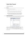
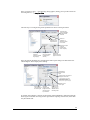
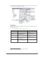
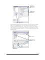
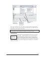
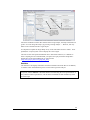
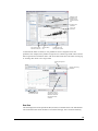
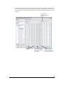
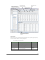
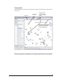
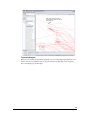
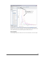
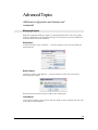
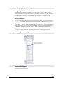
MTE -- Movement Time
Evaluator
.
.
.
.
.
.
.
Tutorial & User Manual
Input Device Usability Evaluation, Education & Research Workbench
Martin Schedlbauer, Ph.D.
[email protected]
[email protected]
.
2
Table of Contents
Introduction _______________________________________________ 5
Availability ________________________________________________ 5
Support ___________________________________________________ 6
Installation ________________________________________________ 6
Windows ____________________________________________________ 6
Linux _______________________________________________________ 6
MacIntosh ____________________________ Error! Bookmark not defined.
Overview __________________________________________________ 7
Configurability _______________________________________________ 8
Evaluation and Analysis _______________________________________ 8
Exporting to Other Tools ______________________________________ 9
Feedback ____________________________________________________ 9
Process __________________________________________________ 10
Configure an Experiment ___________________________________ 10
Target Shapes _______________________________________________ 12
Target Placement Strategies ___________________________________ 13
Collect Data ______________________________________________ 13
Analyze Results ___________________________________________ 15
Merging Result Files _________________________________________ 15
Loading the Data ____________________________________________ 16
Statistics ___________________________________________________ 17
Raw Data __________________________________________________ 18
Model Evaluation ____________________________________________ 20
Width Models __________________________________________________ 21
Model Functions ________________________________________________ 22
Performance Models _____________________________________________ 22
3
Trajectory Plot ______________________________________________ 23
Trajectory Analysis __________________________________________ 24
Ad Hoc Analysis _____________________________________________ 25
Managing Subjects_________________________________________ 26
Add Subject ________________________________________________ 26
Delete Subject _______________________________________________ 26
List Subjects ________________________________________________ 26
Running Experiments Remotely ______________________________ 27
Configuring the Collection Station ______________________________ 27
Running Remotely ___________________________________________ 27
Managing Experimental Data ________________________________ 27
Configurable Options_______________________________________ 27
Searching for Specific Experiments ___________________________ 28
Performing Ad Hoc Analysis _________________________________ 28
Adding New Models ________________________________________ 28
Exporting Data ____________________________________________ 29
Exporting to R and Excel ___________________________________ 29
Exporting as XML _________________________________________ 29
4
Overview
MTE as a research and education
workbench
Introduction
While many specialized utilities have been developed to capture data for evaluating the
usability of input devices, few of these tools are general purpose experimental and educational
platforms. This guide describes the Movement Time Evaluator (MTE), an interactive software
platform for designing, executing, and analyzing Fitts-type experiments. It is an extensible
tool which allows students to focus on discovery and exploration rather than programming. In
addition, it provides students insight into graduate research which may encourage them to
continue their education. We believe that interactive experimentation will make theoretical
concepts more accessible to the students, and we hope will make them aware of scientific
exploration in HCI.
MTE is a configurable tool for exploring input device characteristics as well as rapidly
evaluating performance models. It is written in Java and is constructed on an extensible
object-oriented and pattern-based framework. MTE has a comprehensive graphical user
interface that allows researchers to configure their experiments and interpret results
interactively. It allows researchers to compare their own models immediately to Fitts’ law,
and the variations defined by Accot and Zhai, Kvålseth, MacKenzie, and Meyer et al..
MTE extends Soukoreff and MacKenzie’s platform by adding bivariate pointing tasks, probe
corrections, additional performance models, non-stationary targets, soft keypads, dynamic
configurability, and movement microstructure evaluation. As a result, MTE presents a new
research platform which allows input device investigators to conduct standardized
experiments and to directly compare device characteristics, performance and usability.
Silfverberg, MacKenzie, and Kauppinen lament the fact that between-study comparisons are
not addressed by ISO9241 and that unified test conditions only provide high-level
comparisons of research results. Douglas, Kirkpatrick, and MacKenzie “adamantly assert
caution in comparing results across experiments.” They argue that “it is critical that exactly
the same experimental design, task environment, instructions and data analysis be given” and
that “given these limitations, it is useful to have standardized software.” Sharable
experimental configurations and results are required to carry out between-study statistical
analyses. MTE provides a framework upon which to build a database of reference conditions,
configurations, and eventually experimental results.
Availability
The MTE platform is available under the GNU Public License (GPL) as open source software.
An executable version with an installation wizard that runs under Java 5 or later as well as the
full source code can be downloaded from the web, allowing for modification and extension by
students and researchers. The software has been tested on Windows 98, Windows
2000/NT/XP/Vista/7-32/7-64, Linux, and Mac OS X running Sun Java 5 and later.
Its source code and compiled versions are available for download from:
5
http://research/cathris/com/mte
The web site has a self-installing kit for Microsoft Windows (XP/NT/2000/98/Vista/7) in the
form of an MSI file.
Support
Support is available directly from the author as well as through a forum hosted by Yahoo.
You can contact the tool’s author (Martin Schedlbauer) via e-mail at [email protected]
or [email protected]. The Yahoo group that hosts a discussion forum, mailing list,
downloadable experiment configuration, add-ons, and user contributions, is located at:
http://tech.groups.yahoo.com/group/uml_mte/
Installation
Windows
1.
Download MTE from research.cathris.com/mte. The web site contains a
self-extracting MSI file that installs under Windows
95/98/NT/2000/XP/Vista/7. It has been tested on 32-bit and 64-bit
installations.
2.
Run the downloaded installer and follow the wizard’s directions. On Vista
and Windows 7, change the default installation folder to c:\mte otherwise
you will not be able to run MTE as on Vista and 7 the Program Files
directory is write protected.
3.
Open your start menu, then select Programs, followed by MTE.
4.
When first run, MTE will warn you about not finding a registry file. Click
OK to proceed. A default registry file will be created in which MTE
configuration parameters will be stored.
5.
You are now ready to configure, execute, and analyze experiments.
On a standard Windows installation, the <MTE root> folder is “C:\Program
Files\MTE”. The configurations are stored in <MTE root>/data/configs.
Experiment
results
are
stored
in
automatically
named
files
in
<MTE root>/data/runs. To create additional folders for storing and organizing
experiments or configurations, you need to use your file system’s explorer, e.g.,
Windows Explorer.
On Vista and Windows 7, change the default installation folder to c:\mte otherwise
you will not be able to run MTE. As on Vista and 7 the Program Files directory is
write protected.
Linux and Mac OS X
1.
Download the MTE Java jar file mte.jar from
http://research.cathris.com/mte
2.
Launch a terminal window
6
3.
In your home directory, create a directory called MTE (generally using cd;
mkdir MTE)
4.
Move into that directory (cd MTE) and create a subdirectory in MTE called
data (mkdir data). Move into the data directory (cd data) and create three
additional subdirectories within data called configs, export, and runs (mkdir
configs export runs)
5.
Move back into the main MTE directory and run MTE from the command
line with:
% java -cp mte.jar edu.uml.mte.ui.Main .
6.
If you want to perform remote experiments, you also need the XML file
servers.xml that contains the IP addresses or remote machines on
which experiments are conducted. It must be placed into the data
directory.
7.
Here is a sample servers.xml file:
<?xml version="1.0" encoding="UTF-8"?>
<!DOCTYPE addresses [
<!ELEMENT addresses ( server+ )>
<!ELEMENT server ( #PCDATA )>
<!ATTLIST server
ip CDATA #REQUIRED>
]>
<addresses>
<server ip="192.168.102.176">Tablet PC</server>
<server ip="192.168.102.170">Compaq iPAQ/Elo</server>
</addresses>
8.
When the program first runs it looks for subjects.xml and
registry.xml. If it does not find them, it creates default files. The
subjects.xml file contains subjects for the experiment (configurable
through the Subjects menu in MTE) and registry.xml contains
program settings (configurable through Tools/Options... in MTE.)
Overview
Experiments are interactively configurable and the configurations are saved in a sharable
XML format. The experiments can be carried out via a network allowing the research and
subject to be separated by any distance. Its data sets are saved in either XML or CSV which
simplifies importing into customized programs and off-the-shelf plotting and statistical
packages, such as Microsoft Excel and R1. Furthermore, MTE contains interactive plotting
1
R is an open source statistical package available from http://www.r-project.org.
7
and basic statistical analysis allowing student researchers to collect data and “play with the
data” in a single environment. The tool supports visualization of a single data set, several data
sets side-by-side or overlaid, cursor paths, spatial variability of cursor selection end points,
and cursor kinematics. Lastly, its internal object-oriented architecture makes extensions to the
tool relatively simple.
MTE is based upon a distributed architecture in which a researcher controls experiments from
one workstation while the subjects interact with the software on different workstations. This is
particularly useful for students conducting experiments and collecting data remotely.
The overall platform capabilities are summarized in the UML (Unified Modeling Language)
use case model to the left.
The papers listed in the references section at the end of the manual demonstrate the use of
MTE.
Configurability
Experiments are configured in two steps. The researcher first creates an experiment setup
which specifies session invariant parameters, including target extent, target shape type (oval,
rectangular, moving, or soft keypad), home region placement (center, upper left corner of
screen, or none), target position distribution (reciprocal, pre-programmable, or random),
auditory and visual feedback preferences, number of repetitions, type of movement (pointand-click versus drag-and-drop) and the type of information to be recorded for each aiming
task (cursor path and errors). The saved and sharable configuration files are used in the
second step, which is running the
experiment. The researcher can recall a
previously recorded configuration from a
list of stored setups. Before each
experimental session, input device type,
screen dimension, probe characteristics,
gain settings for the input device, as well as
any other relevant ad hoc information are
recorded. For each subject, demographic
information is collected, including age,
gender, height, and handedness.
MTE can be extended by adding new static
as well as dynamic (moving) shape types,
target position distributions, movement
time models, and data export formats.
Evaluation and Analysis
To assist in the rapid evaluation and
interactive exploration of movement
models and input devices, basic statistical
analysis is built into the platform. The
recorded data can be easily exported to many statistical packages for more sophisticated
analysis. MTE supports correlation analysis and linear regression, as well as configurable
scatter plots and distribution graphs. In addition, the raw data and the trajectory of the
individual acquisition movements during a session can be viewed so that the movement
patterns for different input devices can be studied. Lastly, a table comparing the correlation
coefficients of various movement time models, including Fitts’ law is displayed.
8
The linear regression coefficients and the correlation coefficients can be computed either on
the raw observations or averaged MT values across ranges of ID attenuating the effect of
outliers. A sortable table containing collected trial data can be drawn on to identify outliers.
Exporting to Other Tools
The tool records the experiment configuration and the data for each movement trial in a
persistent and sharable XML document. While the statistical mechanisms built into MTE are
certainly useful, they are limited but easily augmented by specialized statistics packages. The
data can be copied to the clipboard or saved as CSV files for import into Microsoft Excel and
statistical analysis packages, such as R. Although the plotting capabilities of MTE are useful
for interactive exploration, they are not configurable enough for publication. Both R and
Microsoft Excel offer better support in that area.
Feedback
This manual is a continuous work in progress. Your feedback and additions are welcome. If
you would like to edit the manual, please let us know and we will send you the Word file for
modification. You can contact us at [email protected].
9
Quick Start Tutorial
A step-by-step tutorial
Process
Experimentation in MTE is a three-step process:
1.
Configure the experiment parameters and store the configuration settings in
a file.
2.
Load a stored experiment configuration and run the experiment either
locally or remotely (requires installation of MTE on the remote computer).
3.
Merge the results from multiple subjects into a single file, and then load the
result file into MTE for analysis. In addition, you may want to export the
data via CSV to R or Excel for additional statistical analysis and plotting.
Configure an Experiment
Start the configuration process by creating (or modifying) an experiment configuration. Select
“Configure…” from the “Experiment” menu. The following dialog will appear:
In the above dialog, click on the folder in which you wish to store the configuration, then
select “New…”. To create additional folders for storing experiments, you need to use your
file system’s explorer, e.g., Windows Explorer. The configurations are stored in
<MTE root>/data/configs. On a standard Windows installation, the <MTE root>
folder is “C:\Program Files\MTE” but on Windows 7 and Vista it should be changed
during installation.
10
Once you click on “New…”, the following dialog appears, asking you to provide a name for
the configuration, e.g., simple-fitts.
The next step is to configure the general parameters as shown in the figure below.
Click-and-Drag
task (if selected) or
simple point-andclick task
Number of
repetitions, i.e.
selections subject
has to make
Free-form text
description and
experiment title
Record cursor path
(useful for
kinematic and
motion analysis)
Record any error
selections
(selections outside
target region)
Display cursor
trace (only applied
to indirect input
devices)
Defer target
display until home
region is clicked on
Once the general parameters are configured, the home region settings are made. Select the
“Home Region” tab to display those settings:
Text displayed
inside the home
region
Location where home region is
displayed. Choices are:
• Center (centered on the screen)
• Random (randomly placed)
• Origin (upper left corner of screen)
• None (no home region is displayed)
Geometry of the
home region
Emits a sound
upon selection of
the home region
Inverts the
foreground and
background colors
the home region
upon selection
Hides the home
region once it is
selected and the
trial timing starts
If no home region display is chosen, the trial timing starts immediately, rather than when the
home region is selected. Not using a home region allows capturing reaction time, rather than
only movement time.
11
Once the home region parameters are configured, the target region settings are made. Select
the “Target Region” tab to display those settings:
Select the shape
type. Use the “…”
to configure the
shape
Set the target
placement strategy
Target width and
height in pixels. If
the randomize
check boxes are
set, then the width
and height are
varied between 10
and the set extent
Determines how many
“decoy” targets are
displayed in addition to
the actual target
Target selection
parameters
Target Shapes
MTE supports several shapes for the target (any distracter shapes are displayed in the same
shape type as the target):
Table 1: Target shape types and associated description.
2
Shape
Description
Configurable Parameters
RectangularRegion
Rectangular area
width, height, foreground,
background
LabelRegion
Rectangular area with a string
displayed within the area
width, height, text string2
OvalRegion
Oval or circular area
width, height, foreground,
background
VibratingRegion
Rectangular area that moves randomly
in two dimensions to simulate a
moving environment
width, height, amplitude,
frequency (on x and y axis)
Keypad
Numeric keypad with 10 numeric
buttons and two additional buttons
gap between buttons, string to be
entered, visual feedback time (in
ms)
In a future release, the font type and font size will be configurable.
12
Target Placement Strategies
MTE supports several placement (or distribution) strategies for targets:
Table 2: Target placement strategies.
Distribution Strategy
Description
Configurable Parameters
FixedRandomDistribution
Places targets at random locations on the
screen. Every time the experiment is run,
targets will appear in the same locations.
random seed (configurable
through Tools/Options…)
RandomDistribution
Places targets at random locations that
vary each time the experiment is run.
none
ReciprocalDistribution
Places targets along the horizontal
oscillating between the left and right side
of center of the screen. Simulates the
classic Fitts tapping experiment.
none
StaticDistribution
Places targets at pre-programmed
positions. Use the “…” to configure the
target locations.
distance and angle from
center of screen
Save the configuration, by selecting “Save”. Once you are satisfied with your configuration
settings, you can test it by selecting “Test…”. The results are not recorded. You can interrupt
a test by simply dismissing the testing windows. When done, choose “Close”.
Pressing “Close” will dismiss the dialog and not save any changes. So, be sure to press
“Save” if you want your changes to be persistent.
Collect Data
To run as experiment, choose “Run…” from the “Experiment” menu. The following dialog
will appear, allowing you to select a previously stored experiment configuration:
13
Subject that will
complete the experiment
(previously set up
through “Subjects/Add
New…”
Demographic and
environment information
that will be stored for
future reference
Experiment to run
Normally, experiment results are saved in a file. However, you may not wish to save warm-up
trials. To save the experiment results, select “Save Trial Data” and then select a folder in
which to save the results (by pressing the “…” button). In the file dialog, you can create new
folders. We suggest that you save the trials for each subject in a separate folder. For example,
we created folders for each subject, named “1”, “2”, etc. You could also use the subject’s id or
the subject’s initials.
Create new folder
Select folder in which
result file is save, then
press OK
Click to configure folder
in which result file is
placed
Select to save
experiment results
14
Once everything is configured, press “Run” to start the experiment. The following advisory
dialog will appear in the experiment window showing the experiment ID which will also be
the name of the experiment’s result file:
Upon selecting OK, the experiment starts and the home region (if one has been configured)
and the target (unless target deferment has been configured) are displayed. Trial timing starts
upon selection of the home region. If no home region has been configured, trial timing starts
as soon as the target is displayed. The title of experiment window displays the number of
trials remaining.
Repeat this process for each experiment configuration and each subject. Upon collecting all of
the data, the individual experiment results will need to be merged into a single file for
analysis. This process is explained in the next section.
Analyze Results
Merging Result Files
The first step in analysis is the merging of all of the individual result files for each subject into
a single file. To start the process, select “Merge Data Sets…” from the “Tools” menu. This
will bring up the following dialog:
15
Step1: Select the folder
that contains the files. If
the folder contains
subfolders, all files will
be merged recursively
Step3: Specify merge
controls. You can omit
errors selections,
average all results, and
save the data as XML
(not recommended)
Step2: Enter a file name
and folder for the
merged data
Once you have selected the files to merge and have entered a filename for the merged data,
press “Merge”. The process may take a minute or more depending on the number of files and
whether the files contain trajectory information.
Once the merge is complete, we recommend that you select “Refresh Experiment List” from
the “Tools” menu, so that the merged file will appear in the “Run Files” file tree.
Loading the Data
Once the merged file has been prepared, you can load the data in three ways. One, you can
choose “Load…” from the “Experiment” menu and then pick the file
Data files with an
from the dialog. Second, you double-click on the file in the file tree.
extension of .ser
Third, you can single-click on the file in the file tree and then open the
are Java serialized
pop-up menu with the right (unless your mouse is configured for left
objects.
handed use) mouse button and pick “Load”. Regardless which approach
you use, the data is loaded and a summary is displayed in the “Summary” tab. An annotated
example is shown below:
16
The input device is
“unknown” in merged
files. Any of the fields
can be edited. To save
the information back to
the merged file, press
Update
This is the information specified
when the experiment was run
Unless the loaded file contains data collected from a single subject, the subject information is
generic. You can change the subject, by pressing “Change Subject…”. However, this only
makes sense if the data is from a single subject.
It is important to update the Target Shape to any of the valid names shown in Table 1. If not
updated, the “Trajectory Plot” will not display the correct targets.
The next sections will explain the different tabs in more detail. However, it is difficult to
show everything and we recommend that you explore and “play with some sample data”.
Sample data can be downloaded from our Yahoo forum
(http://tech.groups.yahoo.com/group/uml_mte/).
Statistics
The “Statistics” tab displays summative statistical information about the data set. In addition,
it contains scatter and distribution plots as well as linear regression analysis.
In MTE, amplitude refers to the Pythagorean distance between the movement starting and
end points, whereas distance is the actual distance traveled along the cursor path. Distance is
only valid for indirect input devices, such as mouse or trackball. It does not make any sense
for touch input.
17
Distribution of ID,
amplitude, MT, or
distance over the
specified number of
bins
Configure model
parameters
X and Y axis
parameters
Press “Add” to add the
data to the scatter plot
Clear the plotting
area
Correlation (R and R2)
and regression equation
To attenuate the effect of outliers, Y axis parameters can be averaged across X axis
parameters. For example, many studies average MT over a fixed range of ID values to obtain
better regression and correlation results. The screen shot below shows the effect of averaging
or “binning” MT values over a range of IDs.
Display the regression
line
Configure the binning
parameters
Clear any scatter plot
first, then select Add
The number of bins is
generally the number of
different ID values that
the experiment setup
contained
Raw Data
This tab displays the actual experiment data (raw data) in a tabular format. The table headers
can be selected which causes the table to be sorted accordingly. This is useful for detecting
18
outliers. Outliers can be removed from the table by entering the row number at the bottom of
the table. The reduced table can be saved back to the same or a different file. The data set can
be exported to a CSV file if further analysis is to be carried out in another program, such as R
or Excel.
Average data for
matching trials across
subjects
Row to remove from
data set
Save the data set back
to the same or a different
file name after rows have
been removed
Export the entire table as
a comma-separated
values (CSV) file suitable
for import into R or Excel
19
The raw data table displays a number of collected data scores. The meaning of each value is
explained in Table 3:
Table 3: Collected data values
Value
Description
Row
The row number; needed for deleting a row when scrubbing the
data
SID
The subject identifier
MT
Movement time/trial completion time
ST
Starting time (in Java ticks)
ET
End time (in Java ticks)
A
Amplitude of movement (distance from home center to target
center)
A’
Alternative amplitude of movement (distance from starting point
to end point)
A(mm)
Amplitude as A’ except in millimeters
D
Distance traveled along the cursor path for indirect input devices
Angle
Angle between center of home region and center of target
TW
Target width
TH
Target height
ID
The Fitts Index of Difficulty (according to MacKenzie’s
formulation)
Errors
Number of selections outside the target
MV
Movement variability: the average least square distance between
the ideal path to target versus the actual path traveled; measures
the “jigginess” of the movement
Reference
Fitts (1954), MacKenzie
(1991)
MacKenzie et al. (2001)
Model Evaluation
The “Model Evaluation” tab displays correlation and regression results for a number of
different performance models, including various formulations of Fitts’ law. Some of the
models can be configured by pressing the header column in the model table. In addition,
various width and amplitude values can be applied. The regression and correlation results can
be calculated on the raw and on averaged (binned) data similar to the scatter plot in the
“Statistics” tab.
A second table shows statistical data for each target, including the effective target width (We)
and the standard deviation of the target end points from the mean and the target center. The
effective width is an indicator of how subjects actually perform the experiment. Some
subjects move more deliberately and slower therefore they have a lower error rate, while
others move faster but with less accuracy. See the papers by MacKenzie and Schedlbauer for
additional background information.
20
Add the probe width in
Determine if amplitude is from
touch input to the width
starting point to end point of
movement or from home center to
Perform a log-transform
target center
on MT to normalize the
Omit outliers from the
analysis
distribution
Average the ID to
attenuate outliers
Export the effective width and SD
data to a CSV file for import into R
and Excel
Width Models
MTE supports a variety of width calculation approaches. There is generally agreed upon way
on how to calculate width for a bivariate pointing task.
Table 4: Width calculation approaches
Width Model
Description
Reference
2D Width
Width along the approach vector
MacKenzie
Horizontal Extent
Target size along the horizontal (width)
MacKenzie, Fitts
Smaller of {W,H}
Smaller of target width or height
MacKenzie
Area
Geometric area of the target
MacKenzie,
Schedlbauer
Sum of {W,H}
The sum of width and height
MacKenzie
We
Effective width
MacKenzie
21
Model Functions
For each model, the following functions are calculated and displayed in the table:
Table 5: Functions calculated for each performance model
Function
Description
Reference
R(A,W)
Correlation coefficient (R) based on the amplitude and the selected
width model
R(D,W)
Correlation coefficient (R) based on the distance (actual cursor path)
and the selected width model
R2 (A,W)
Coefficient of determination (R2) based on the amplitude and the
selected width model
R2 (D,W)
Coefficient of determination (R2) based on the distance (actual cursor
path) and the selected width model
1/b
Throughput based on the inverse of the regression slope
Zhai, MacKenzie
TP-A
Throughput based in the ratio of averaged MT/ID where ID is
calculated based on the amplitude
MacKenzie, ISO
TP-D
Throughput based in the ratio of averaged MT/ID where ID is
calculated based on the distance
Mean(ID)
The average ID in the data set
Max(ID)
The maximum ID in the data set
Min(ID)
The minimum ID in the data set
Mean(MT)
The average MT in the data set
Max(MT)
The maximum MT in the data set
Min(MT)
The minimum MT in the data set
Intercept
The intercept value of the linear regression equation for the model
Fitts, MacKenzie
Slope
The slope value of the linear regression equation for the model
Fitts
Performance Models
MTE calculates the above values for the following movement time models. Clicking on the
model name in the table header will display the model equation, reference, and any adjustable
parameters. In the table below, A is the amplitude and W is the width according to the
calculation approaches that were selected.
Table 6: Fitts models supported by MTE
Model
Description
Simple
A/W
Fitts
log2(2A/W)
Fitts (1954)
Welford
log2(A/W + 0.5)
Welford (1960)
Shannon
log2(A/W + 1)
MacKenzie (1991)
Meyer
sqrt(A/W) [simplified version of the generalized model]
Meyer et al. (1988)
c
Kvålseth
(A/W)
Accot-Zhai
(see paper)
ID^2
[log2(A/W + 1)]2
Reference
Kvalseth (1980)
Accot & Zhai (2003)
22
Trajectory Plot
This tab displays the actual selection end points, optionally with target outlines and the actual
cursor path.
Zoom slider
Display target
outlines
Display direct path
from home to target
as well as actual path
traveled
Show error selections (open circles)
Load another data set and display it
along with the current data set.
Useful for comparing relative
accuracy of input devices
Below is an example of a zoomed display showing the cursor path (trajectory) for a small data
set. Showing the trajectory for large data sets is computationally slow and visually cluttered.
23
Path of the cursor from home to
target (only appropriate for indirect
input devices)
Trajectory Analysis
Here you can visualize the speed-time graph for a set or an individual target acquisition. You
need to enter the run number which you can get from the raw data table or the “Trajectory
Plot” when displaying the ideal path.
24
Speed-vs-time graph for a range of
runs; the range must be
consecutive and specified as a-b
Selecting “Show Mean Curve” will display a curve that represents the average values of a set
of runs. Smoothing the curve attenuates the peaks and valleys of the curve.
Ad Hoc Analysis
This tab displays output from custom Java code. For more information, see the next chapter.
25
Advanced Topics
Additional configuration mechanisms and
commands
Managing Subjects
MTE allows individual tracking of subjects, so that experimental factors such as age, height,
gender, or handedness can be included in the analysis. All subjects are stored in an XML file
in the data folder of the MTE installation.
Add Subject
To add a new subject, select “Add New…” from the “Subjects” menu. This will display the
following dialog:
Delete Subject
To remove a subject, select “Remove…” from the “Subjects” menu. This will cause the
following dialog to appear:
Select the subject from the list and press OK to remove that subject.
List Subjects
To see all of the subjects, select “List all” from the “Subjects” menu. A dialog with a list of all
of the subjects will be displayed.
26
Running Experiments Remotely
Configuring the Collection Station
Install MTE on the experiment workstation as well as on the researcher’s control station.
Installation is done in the same way on both. On the remote station (the one where the subject
will perform the trials), choose “Launch Remote Server” from the “Tools” menu. The
experiment canvas will appear and wait for an experiment to be sent to it by the researcher.
Running Remotely
You will need to add the IP address of the experiment workstation (the remote station) to the
servers.xml file in the data folder of the MTE installation folder. Alternatively, you can
type it into the “Choose Server” field in the Run dialog. To run an experiment remotely,
choose “Run…” from the “Experiment” menu. In the “Choose Server” field, simply select the
remote workstation or type in its IP address or domain name. The experiment will then start
on the remote machine assuming that its remote server was launched as explained in the
section above. Note that you can select more than one experiment from the Run dialog in
which case all of the experiments are run in sequence. The subject can rest before each
experiment by simply waiting to click OK on the instruction dialog.
Managing Experimental Data
Move (cut), copy, rename and
delete files. Add new folders.
Configurable Options
This section needs to be written.
27
Searching for Specific Experiments
This section needs to be written.
Performing Ad Hoc Analysis
This section needs to be written.
Adding New Models
This section needs to be written.
28
Exporting Data
Export your data to other programs for
analysis and plotting
Exporting to R and Excel
To be written…
Exporting as XML
The data files are savable in two formats. All data collected during an individual run of an
experiment is saved as an XML file.
When files are merged, for performance reasons the default format is a Java serialized object.
However, when you merge experiment files, you can select “Save as XML” in the Data
Options section of the merge dialog (accessed via Tools/Merge Data Sets…).
29
References
Papers and reports containing background
theory and results obtained with MTE
Accot, J., & Zhai, S. (2003). Refining Fitts’ law models for bivariate pointing. In Proceedings
of the ACM CHI 2003 Conference on Human Factors in Computing Systems, April 2003, Ft.
Lauderdale, FL: ACM, 193-200.
Fitts, P. M. (1954). The information capacity of the human motor system in controlling the
amplitude of movement. Journal of Experimental Psychology, 47, 381-391.
Kvålseth, T. (1980). An alternative to Fitts’ law. Bulletin of the Psychonomic Society, 16(5),
371-3.
MacKenzie, S. (1991). Fitts' law as a performance model in human-computer interaction.
Unpublished Doctoral Dissertation, University of Toronto, Department of Computer Science,
Toronto, Canada.
MacKenzie, S., & Buxton, W. (1992). Extending Fitts’ law to two-dimensional tasks.
Proceedings of the ACM Conference on Human Factors in Computing Systems - CHI '92,
219-226. New York: ACM.
MacKenzie, S. (1995). Movement time predictions in human-computer interfaces. In
Readings in Human-Computer Interaction, 2nd Edition, Morgan Kaufman, Los Altos, CA,
483-493.
MacKenzie, I. S., Kauppinen, T., & Silfverberg, M. (2001). Accuracy measures for evaluating
computer pointing devices. In Proceedings of the ACM Conference on Human Factors in
Computing Systems - CHI 2001, 9-16. New York: ACM.
Meyer, D., Abrams, R., Kornblum, S., Wright, C., & Smith, J. (1988). Optimality in human
motor performance: Ideal control of rapid aimed movements. Psychological Review, 95:3,
340-370.
Meyer, D. E., Smith, J. E. K., Kornblum, S., Abrams, R. A., & Wright, C. E. (1990). Speedaccuracy tradeoffs in aimed movements: Toward a theory of rapid voluntary action. In M.
Jeannerod (Ed.), Attention and performance XIII. Hillsdale, NJ: Lawrence Erlbaum, 173-226.
Schedlbauer, M. (2010). Effects of Design on the Completion Time and Accuracy of Input
Tasks on Soft Keypads using Trackball and Touch Input. Submitted to Journal of Usability
Studies.
Holzinger, A., Höller, M., Schedlbauer, M., & Urlesberger, B. (2008). Fitts’ Law in Real Life
Medical Scenarios: Performance of Finger versus Stylus. In Proceedings of Information
Technology Interfaces (ITI 2008), Dubrovnik, Croatia, July 2008.
30
Schedlbauer, M., & Heines, J. (2007). Selecting While Walking: An Investigation of Aiming
Performance in a Mobile Work Context. In Proceedings of the 13th Americas Conference on
Information Systems (AMCIS), Keystone, Colorado, August 9-12, 2007 (Recipient of Best
HCI Paper, Best Conference Paper Honorable Mention).
Schedlbauer, M. (2007). Completion Time Predictions of Touch-Screen Interactions in DualTask Situations. In Proceedings of the 29th Annual Conference on Information Technology
Interfaces (ITI 2007), Dubrovnic, Croatia, June 2007.
Micire, M., Schedlbauer, M., & Yanco, H. (2007). Horizontal Selection: An Evaluation of a
Digital Tabletop Device. In Proceedings of the 13th Americas Conference on Information
Systems (AMCIS), Keystone, Colorado, August 9-12, 2007.
Schedlbauer, M. (2007). Effects of Key Size and Spacing on the Completion Time and
Accuracy of Input Tasks on Soft Keypads using Trackball and Touch Input. In Proceedings of
the Human Factors & Ergonomics Society 51st Annual Meeting, Baltimore, MD, October,
2007.
Pastel, R., Champlin, H., Harper, M., Paul, N., Helton, W., Schedlbauer, M., & Heines, J.
(2007). The Difficulty of Remotely Negotiating Corners. In Proceedings of the Human
Factors & Ergonomics Society 51st Annual Meeting, Baltimore, MD, October, 2007.
Schedlbauer, M. (2007). A Configurable Platform for the Interactive Exploration of Fitts’
Law and Related Movement Time Models. Extended Abstracts of the ACM Conference on
Human Factors in Computing Systems (CHI 2007), San Jose, CA, April 2007.
Schedlbauer, M., Pastel, R., & Heines, J. (2006). Effect of Posture on Target Acquisition with
a Trackball and Touch Screen. In Proceedings of 28th Annual Conference on Information
Technology Interfaces (ITI 2006), Dubrovnic
Schedlbauer, M. (2007). A Survey of Manual Input Devices. Technical Report 2007-002,
Computer Science Department, University of Massachusetts, Lowell, MA.
Schedlbauer, M. (2007). A Survey of Human Cognitive and Motor Performance Models.
Technical Report 2007-001, Computer Science Department, University of Massachusetts,
Lowell, MA.
Schedlbauer, M. (2006). An Empirically Derived Model for Predicting Completion Time of
Cursor Positioning Tasks in Dual-Task Environments. Doctoral Dissertation, Department of
Computer Science, University of Massachusetts Lowell, April 2006.
Schedlbauer, M., Heines, J. (2005). An Extensible and Interactive Research Platform For
Exploring Fitts' Law. Technical Report 2005-015, Computer Science Department, University
of Massachusetts, Lowell, MA.
Soukoreff, W., and MacKenzie, I. S. (1995). Generalized Fitts' Law Model Builder. In
Proceedings of the ACM Conference on Human Factors in Computing Systems – CHI 1995.
ACM Press, 113-114.
University of Oregon HCI Research Laboratory. WinFitts: Two-dimensional Fitts
Experiments on Win32. http://www.cs.uoregon.edu/research/hci/research/winfitts.html.
31
Welford, A. (1960). The measurement of sensory-motor performance: Survey and reappraisal
of twelve years’ progress. Ergonomics, 3, 189-230.
32