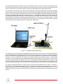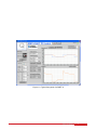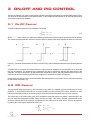
1
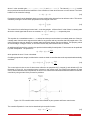
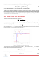
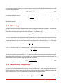
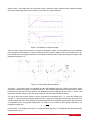
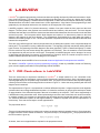
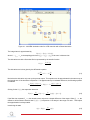
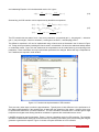
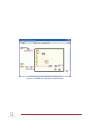
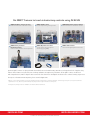
Practical Control Guide QNET Trainer for NI ELVIS Developed by: Karl Johan Åström, Ph.D., Lund University (Emeritus) Jacob Apkarian, Ph.D., Quanser Michel Lévis, M.A.Sc., Quanser Powered by: Captivate. Motivate. Graduate. © 2011 Quanser Inc., All rights reserved. Quanser Inc. 119 Spy Court Markham, Ontario L3R 5H6 Canada [email protected] Phone: 1-905-940-3575 Fax: 1-905-940-3576 Printed in Markham, Ontario. For more information on the solutions Quanser Inc. offers, please visit the web site at: http://www.quanser.com This document and the software described in it are provided subject to a license agreement. Neither the software nor this document may be used or copied except as specified under the terms of that license agreement. All rights are reserved and no part may be reproduced, stored in a retrieval system or transmitted in any form or by any means, electronic, mechanical, photocopying, recording, or otherwise, without the prior written permission of Quanser Inc. QNET User Manual 2 CONTENTS 1 Introduction 4 2 Control Practice 7 3 On-off and PID Control 3.1 On-Off Control 3.2 PID Control 3.3 Peak Time and Overshoot 3.4 Filtering 3.5 Set-Point Weighting 3.6 Integral Windup 9 9 9 11 12 12 13 4 LabVIEW 4.1 PID Controllers in LabVIEW 16 16 QNET User Manual v 1.0 1 INTRODUCTION Feedback has many useful properties, for example: it permits design of good systems from poor components, unstable systems can be stabilized, and effects of disturbances can be reduced. Combining these nice properties with the advances in computing and software, which has made design simpler and implementation cheaper, it is easy to understand why applications of control are expanding rapidly. The concepts of control are also essential for understanding natural and man-made systems. A recent panel [5] gives the following recommendation: Invest in new approach to education and outreach for the dissemination of control concepts and tools to nontraditional audiences. The panel report goes on to say: As a first step toward implementing this recommendation, new courses and textbooks should be developed for experts and non experts. Control should also be made a required part of engineering and science curricula at most universities including not only mechanical, electrical, chemical, and aerospace engineering, but also computer science, applied physics and bioengineering. It is also important that these courses emphasize the principles of control rather than simply providing the tools that can be used for a given domain. An important element of education and outreach is the continued use of experiments and the development of new laboratories and software tools. This is much easier to do than ever before and also more important. Laboratories and software tools should be integrated into the curriculum. The laboratories described in this book are designed to implement some of the recommendations. Since control is a systems field, to get a full appreciation of control it is necessary to cover both theory and applications. The skill base required in control includes modeling, control design, simulation, implementation, commissioning, tuning, and operation of a control system [5], [2]. Many tasks can be learned from books and computer simulations but laboratory experiments are necessary to obtain the full range of skills and a deeper understanding. The experiments in this book can be used in a self-contained course. They can also be used to augment traditional text books such as [6], [1], [3] and [7] with laboratories. The experiments can be used in many different ways, in structured classes as well as for demonstrations and for self-study. Further, they can be used to give students from science and biology an introduction to control. A careful selection was made to obtain a set of experiments that illustrate essential ideas, typical processes and applications. Process control and motion control are two common application areas. In process control a typical task is to keep a process variable constant in spite of disturbances. This type of problem is called a regulation problem. In motion control a typical task is to make an object move in a specified manner. This task is called a servo problem. Typical examples of regulation are found, in process industries such as petrochemical and pulp-and paper, in heating ventilation and air-conditioning, and in laboratory systems. In process control it is often difficult or time consuming to develop mathematical models of the processes. The information required to control the process is therefore often deduced directly by experiments on the process. Controllers can also be installed and tuned by experiments without resorting to a model. We have chosen a heating process as a typical process to illustrate regulation problems. Typical examples of motion control are found in the manufacturing industry, in scanners, printers, cameras, robots, CD players, vehicles, and instrumentation. A characteristic feature of motion control is that it is often possible to obtain mathematical models of the systems from first principles, possibly with a few complementary experiments. We have chosen a simple DC motor to illustrate motion control. Typical experiments are to control the speed or the motor angle in desired ways. Even if there are many applications of regulation and servoing, there are many other types of control problems. Stabilization of an unstable system is one task, the transporter Segway is a typical example. Damping of a swinging load on a crane, motion planning for a moving robot, traction control of cars are other examples. These control tasks are typically more difficult than regulation and servoing and they may require more advanced modeling and control. In spite of this we judged that it was important to have a simple demonstration of task-based control. We have chosen a rotary pendulum and a vertical take-off and landing device as examples of task-based control. The pendulum is a classic system that has been used to teach dynamics and control for a long time. Even if the processes are simple they illustrate many real-life control systems. The vertical take-off and landing device presents a different set of modeling and control challenges geared towards aerospace applications. Although it does involve controlling an actual device, instrumentation is a very important aspect in controls. This involves understanding how to use different types of sensors and switches. Various sensors are found in all types QNET User Manual 4 of industry. Magnetic field transducers are used to detect the throttle in vehicles. Sonar and infrared sensors are often used in mobile robots to measure the distance of surrounding objects. We have chosen a mechatronic sensors device to illustrate how to use different types of sensors as well as switches and light-emitting diodes. The processes are controlled using a PC running the National Instruments programming environment LabVIEW. These processes are manufactured by Quanser and are called Quanser Engineering Trainers for NI ELVIS, or QNET for short. The processes are connected to the computer using the National Instruments Educational Laboratory Virtual Instrumentation Suite (NI ELVIS). As shown in Figure 1.1, the QNET board slides into the NI ELVIS II device. The QNET is compatible with the ELVIS II. The NI ELVIS II has its own DAQ device that connects to the PC via USB. Using LabVIEW it is possible to implement user interfaces that are easy to used. For example, Figure 1.2 shows the front panel for the PI Control of the QNET HVAC Trainer process. It is also possible to look under the hood and see precisely how the controllers and the user interface are implemented. Figure 1.1: NI ELVIS II with ROTPEN Setup The experiments can be performed in many different ways but there are two extremes: the traditional laboratory mode and the guide mode. The traditional mode is to have pre-lab assignments, lab execution, and report writing. It is the more analytical and detailed approach. In the more intuitive guide mode, the laboratories involve immediately running the VI for the experiment and following a procedure outlined in the laboratory manual. The laboratory manuals is a set of brief step-by-step instructions that takes the user through some experiments. It also includes exercises to test the student. The guide mode is also recommended for quick demonstrations (for instance, using a projector) and for students who can work with less structured instruction. Intermediate forms of instruction can be made by combining the modes. Some experiments can be made in guide mode and others in the traditional mode. The manual is organized as follows. Section 2 gives a few hints about practical issues in control. In Section 3, an overview of on-off and PID controllers is given. This material is essential for the experiments, but it can be replaced with similar material in the textbooks that the students use. Section 4 is a short introduction to LabVIEWr . It demonstrates how controllers can be implemented in LabVIEW and how LabVIEW can be used to simulate control systems. QNET User Manual v 1.0 Figure 1.2: Typical front panel of a QNET VI QNET User Manual 6 2 CONTROL PRACTICE Control is a well developed discipline with a good design methodology that is well supported by software. A control system consists of a process, sensors, actuators and a controller. The control law is an algorithm which describes how the signal sent to the actuator are obtained by processing the signals from the sensors. The control algorithm is typically specified as a differential- or a difference equation. The control algorithm is typically implemented as a program in the computer. It is highly advantageous to make an integrated design of the complete system including process design, location of sensors and actuators. However, a control engineer if often asked to control a process with specified sensors and actuators. There are two different approaches to obtain a practical solution to a control problem: empirical or analytical. tuning. When using empirical tuning a standard controller is connected to the sensors and actuators and the parameters are obtained by empirical adjustment. In analytical tuning a mathematical model of the process is first developed and the control algorithm is then obtained by a variety of analytical procedures. In practice it is quite common that the two approaches are combined. Even if empirical tuning is used it is essential to know the system well before control is attempted. Although practicing industrial control engineers do not typically derive models of the system, they are controlling (the authors have seen heuristic manual tuning performed in some of the most demanding applications). This experiment stresses the importance of "knowing the system before you control it". This is also necessary to have a broader understanding of control. The students derive the theoretical open-loop model of the system and assess its performance limitations. The system is designed in such a way that a good model can be derived from first principles. The physical parameters can all be determined by simple experiments. Using VIs and the QNET, the students perform experiments with its inputs and observe its outputs. Open-loop tests are performed and system parameters are estimated using static and dynamic measurements. A first-order simulation of the derived model is run in parallel with the actual system and a bump-test is performed to assess the validity of the estimated model. The procedure used when applying empirical tuning can be summarized in the following steps: • Understand the system • Choose a controller and connect it to the system • Commission the system • Run and evaluate The crucial step in empirical tuning is to choose the control algorithm. A first cut of this choice is very easy because fortunately a PI or PID controller is often sufficient at least for processes with one input and one output. It is therefore important that any user of control has a good understanding of the PID controller. This is the reason why the PID controller is covered extensively in the experiments. Design of more complex controllers require more knowledge than is covered in introductory courses in control. Design of such controllers is however simplified by the availability of good software. Experience indicates that it is difficult to adjust more than two parameters empirically. This is one reason why most industrial controllers are based on PI control, derivative action is used rarely. Analytical tuning can be described by the following steps • Understand the system • Develop a mathematical model • Design a controller • Simulate and validate • Implement the controller • Commission the system QNET User Manual v 1.0 • Run and evaluate Analytical tuning has more steps and is more complicated. However, it has the significant advantage that it is possible to find the factors that limits the achievable performance. When using empirical tuning we never know if it is possible to get better results by using a more complicated controller. Traditional control courses give much emphasis on design of controllers, they also cover modeling and simulation. Availability of systems like LabVIEW makes it very easy to implement controllers because there are standard blocks for PID control. A controller specified by a differential equation or a difference equation can also be implemented easily. Notice that there are several steps in both empirical and analytical tuning that are not covered in typical control courses, namely • Understand the system • Commission the system • Run and evaluate The purpose of this book and the associated experiments are to cover these aspects. Since control covers so many fields the first step is very domain dependent. In this particular case we require that the students develop a good understanding of the particular laboratory systems. This is also a good opportunity to review other courses in engineering. Control is a systems subject. It is when a system has to be commissioned that all pieces of a system come together and it is a challenge to make sure that everything works. To commission a system it is necessary to have a good understanding of all the elements, process, sensor, computer, software and actuator. Commissioning a large system can be quire a scary task, but when it is mastered it also gives the engineer a lot of pride: I made it work! A system seldom works the first time and it is necessary to develop skills in finding the faults. Large companies have engineers who specialize in this task. Control laboratories can be a good introduction to commissioning. Commissioning is a typical skill that is best learned in the tutor/apprentice mode. A few guidelines can be given. A good system should have a stop button so that it can be immediately disconnected if something goes wrong. To start with it is useful to make sure that the control signals are influencing the plant and that the sensors give reasonable signals. For stable systems it is a good idea to make small changes in the control variable in open loop and to observe how the system and the signals react. Make sure that all signs are correct. If the loop is broken at the controller output you can also see how the controller is reacting to the signals. Finally the loop can be closed, with small controller gains. The system can be gently prodded by changing reference values and disturbances. QNET User Manual 8 3 ON-OFF AND PID CONTROL The idea of feedback is to make corrective actions based on the difference between the desired and the actual value. This idea can be implemented in many different ways. In this chapter we will describe on-off and PID control which are common ways to use feedback. 3.1 On-Off Control A simple feedback mechanism can be described as follows: { umax if e > 0 u= umin if e < 0 (3.1) where e = r −y is the control error which is the difference between the reference signal and the output of the system. The control law implies that the maximum corrective action is always used, which explains the name on-off control. Figure 3.1: Controller characteristics for ideal on-off control (A), and modifications with dead zone (B) and hysteresis (C). A system with on-off control will always oscillate, in many cases the amplitude of the oscillations is so small that they can be tolerated. The amplitude of the oscillations can also be reduced by changing the output levels of the controller. This will be discussed in [4] which deals with temperature control. The relay characteristics of the on-off controller can also be modified by introducing a dead-zone or hysteresis, as shown in Figure 3.1. On-off control can also be used to obtain information about the dynamics of a process. This is used in the auto-tuner for PID control discussed in [4]. 3.2 PID Control The proportional-integral-derivative, or PID, controller is very useful. It is capable of solving a wide range of control problems. It is quoted that about 90% of all control problems can be solved by PID control. Moreover, a good majority these problems can be solved using only PI controllers because derivative action is not so common. The reason why on-off control often gives rise to oscillations is that the system over-reacts, a small change in the error will make the manipulated variable change over the full range. This effect is avoided in proportional control where the characteristic of the controller is proportional to the control error for small errors. This can be achieved by making the control signal proportional to the error umax if e > emax u = ke if emin ≤ e ≤ emax umin if e < emin QNET User Manual v 1.0 where k is the controller gain, e = r − y, emin = umin /k, and emax = umax /k. The interval (emin , emax ) is called the proportional band because the behaviour of the controller is linear when the error is in this interval. The linear behavior of the controller is simply u = k(r − y) = ke (3.2) Proportional control has the drawback that the process variable often deviates from its reference value. This can be avoided by making the control action proportional to the integral of the error ∫t u(t) = ki (3.3) e(τ )dτ 0 This control form is called integral control and ki is the integral gain. It follows from 3.3 that if there is a steady state where the control signal and the error are constant, i.e. u(t) = u0 and e(t) = e0 respectively then u0 = ki e0 t This equation is a contradiction unless e0 = 0 and we have thus proven that there is no steady state error if there is a steady state. Notice that the argument also holds for any process and any controller that has integral action. The catch is that there may not always be a steady state because the system may be oscillating. This property, which we call the Magic of Integral Control, is one of the reasons why PID controllers are so common. An additional refinement of the controller is to provide it with an ability for anticipation. Future errors can be predicted by linear extrapolation. The predictor is de(t) e(t + Td ) ≈ e(t) + Td , dt which predicts the error Td time units ahead. Combining proportional, integral, and derivative control we obtain a controller that can be expressed mathematically as follows ∫t de(t) u(t) = ke(t) + ki e(τ )dτ + kd (3.4) dt 0 The control action is thus a sum of three terms referred to as proportional (P), integral (I) and derivative (D). As illustrated in Figure 3.2, the proportional term is based on the present error, the integral term depends on past errors, and the derivative term is a prediction of future errors. Advanced model-based controllers differ from the PID controller by using a model of the process for prediction. Figure 3.2: PID controller takes control action based on past, present and future control errors. The controller Equation 3.4 can also be described by the transfer function C(s) = ks + ki + kd s s (3.5) QNET User Manual 10 Further, it is common in industry to parametrize the PID control in Equation 3.4 as follows ∫t 1 de(t) u(t) = k e(t) + e(τ )dτ + Td Ti dt (3.6) 0 where k is the proportional gain, Ti is the integral time, and Td is the derivative time. The PID controller described by Equation 3.4 or Equation 3.5 is the ideal PID controller. Attempts to implement these formulas do not lead to good controllers. Most measurement signals have noise and taking the differentiation of a noisy signal gives very large fluctuations. In addition, many actuators have limitations that can lead to integrator windup. In addition, the response to reference signals can be improved significantly by modifying the controller. These effects will now be discussed separately. 3.3 Peak Time and Overshoot The standard second-order transfer function has the form Y (s) ωn2 = 2 R(s) s + 2ζωn s + ωn2 (3.7) where ωn is the natural undamped frequency and ζ is the damping ratio. The properties of its response depend on the values of the ωn and ζ parameters. Consider when a second-order system, as shown in Equation 3.7, is subjected to a step input given by R0 R(s) = (3.8) s with a step amplitude of R0 = 1.5. The system response to this input is shown in Figure 3.3, where the red trace is the response (output), y(t), and the blue trace is the step input r(t). Figure 3.3: Standard second-order step response. The maximum value of the response is denoted by the variable ymax and it occurs at a time tmax . For a response similar to Figure 3.3, the percent overshoot is found using PO = 100 (ymax − R0 ) R0 (3.9) From the initial step time, t0 , the time it takes for the response to reach its maximum value is tp = tmax − t0 QNET User Manual (3.10) v 1.0 This is called the peak time of the system. In a second-order system, the amount of overshoot depends solely on the damping ratio parameter and it can be calculated using the equation ) ( P O = 100 e − √π ζ 1−ζ 2 (3.11) The peak time depends on both the damping ratio and natural frequency of the system and it can be derived that the relationship between them is π √ tp = (3.12) ωn 1 − ζ 2 Generally speaking then, the damping ratio affects the shape of the response while the natural frequency affects the speed of the response. 3.4 Filtering A drawback with derivative action is that differentiation has very high gain for high frequency signals. This means that high frequency measurement noise will generate large variations of the control signal. The effect of measurement noise can be reduced by replacing the derivative action term kd s in Equation 3.5 by Da = − kd s 1 + Tf s This can be interpreted as an ideal derivative that is filtered using a first-order low-pass filter system with the time constant Tf . For small s the transfer function is approximately kd s and for large values of s it is equal to kd /Tf . Thus the approximation acts as a derivative for low-frequency signals and as a constant gain of kd /Tf for the highfrequency signals. The filtering time is chosen as kd Td = kN N where N in the range of 2 to 20. The transfer function of a PID controller with a filtered derivative is C(s) = k + ki kd s + s 1 + Tf s The high-frequency gain of the controller is k (1+N ), which is a significant improvement over the ideal PID controller. Instead of only filtering the derivative, it is also possible to use an ideal controller and filter the measured signal. The transfer function of such a controller using a second-order filter is then C(s) = k + ksi + kd s 1 + Tf s + 12 Tf2 s2 (3.13) 3.5 Set-Point Weighting The controllers described so far are called controllers with error feedback because the control action is based on the error, which is the difference between the reference r and the process output y. There are significant advantages to have the control action depend on the reference and the process output and not just on the difference between this signals. A simple way to do this is to replace the ideal PID controller in Equation 3.4 with ∫t u(t) = k(bsp r(t) − y(t)) + ki (r(τ ) − y(τ )dτ − kd dy(t) dt (3.14) 0 QNET User Manual 12 where the parameter bsp is called set-point weight or the reference weight. In this controller the proportional action only acts on a fraction bsp of the reference and there is no derivative action on the set-point. Integral action continues to act on the full error to ensure the error goes to zero in steady state. Closed-loop systems with the ideal PID controller Equation 3.4 or the PID controller with set-point weighting in 3.14 respond to disturbances in the same way, but their response to reference signals are different. Figure 3.4: Set-point weighting effect on step response. Figure 3.4 illustrates the effects of set-point weighting on the step response of the process, P (s) = 1 s with the controller gains kp = 1.5 and ki = 1. As shown in Figure 3.4, the overshoot for reference changes is smallest for bsp = 0, which is the case where the reference is only introduced in the integral term, and increases with increasing bsp . The set-point weights in Figure 3.4 are: bsp = 0 on the bottom dashed plot trajectory, bsp = 0.2 and bsp = 0.5 on the two solid lines, and bsp = 1 on the top dash-dot response. The set-point parameter is typically in the range of 0 to 1. 3.6 Integral Windup Many aspects of a control system can be understood from linear models. There are, however, some nonlinear phenomena that are unavoidable. There are typically limitations in the actuators: a motor has limited speed, a valve cannot be more than fully opened or fully closed, etc. For a control system with a wide range of operating conditions, it may happen that the control variable reaches the actuator limits. When this happens the feedback loop is broken and the system runs in open loop. The actuator remains at its limit independently of the process output as long as the actuator remains saturated. If the integral term is large, the error must change sign for a long period before the integrator winds down. The consequence is that there may be large transients. This phenomena is called integrator windup and it appears in all systems with actuator saturation and controllers having integral action. The windup effect is illustrated in Figure 3.5 by the dashed red line. The initial reference signal is so large that the actuator saturates at the high limit. The integral term increases initially because the error is positive. The output reaches the reference at around time t = 4. However, the integrator has built-up so much energy that the actuator remains saturated. This causes the process output to keep increasing past the reference. The large integrator output that is causing the saturation will only decrease when the error has been negative for a sufficiently long time. When the time reaches t = 6, the control signal finally begins to decrease while the process output reaches its largest value. The controller saturates the actuator at the lower level and the phenomena is repeated. Eventually the output comes close to the reference and the actuator does not saturate. The system then behaves linearly and QNET User Manual v 1.0 settles quickly. The windup effect on the process output is therefore a large overshoot and a damped oscillation where the control signal flips from one extreme to the other as in relay oscillations. Figure 3.5: Illustration of integrator windup. There are many ways to avoid windup, one method is illustrated in Figure 3.6 The system has an extra feedback path that that sets the integrator to a value so that the controller output is always close to the saturation limit. This is accomplished by measuring the difference es between the actual actuator output and feeding this signal to the integrator through gain 1/Tr . Figure 3.6: PID controller with anti-windup The signal es is zero when there is no saturation and the extra feedback loop has no effect on the system. When the actuator saturates, the signal es is different from zero. The normal feedback path around the process is broken because the process input remains constant. The feedback around the integrator will act to drive es to zero. This implies that controller output is kept close to the saturation limit and integral windup is avoided. The rate at which the controller output is reset is governed by the feedback gain, 1/Tr , where the tracking time constant, Tr , determines how quickly the integral is reset. A long time constant gives a slow reset and a short time constant a short reset time. The tracking time constant cannot be too short because measurement noise can cause an undesirable reset. A reasonable compromise is to choose Tr as a fraction of the integrator reset time Ti for proportional control and √ Tr = Ti Td for PID control. The integrator reset time Ti and the derivative reset time Td are defined in the parametrized PID controller shown in 3.6. QNET User Manual 14 The solid curves in Figure 3.5 illustrates the effect of anti-windup. The output of the integrator is quickly reset to a value such that the controller output is at the saturation limit, and the integral has a negative value during the initial phase when the actuator is saturated. Observe the dramatic improvement of using windup protection over the ordinary PI controller that is represented by the dashed lines in Figure 3.5. QNET User Manual v 1.0 4 LABVIEW LabVIEWr is a graphical programming environment that was originally developed by National Instruments to implement virtual instruments. The basic idea was to describe how data flows from a sensor to a display and to quickly generate nice looking displays. LabVIEW which first appeared in 1986 has been developed continuously, currently substantial efforts are made to make extensions to control applications. A key feature is that programming is done graphically by cut-and-paste and that the user interface is an integral part of the system. LabVIEW programs, called VI's (Virtual Instruments), consists of two parts called the front panel and the block diagram. The front panel is the graphical user interface which has indicators, dials and knobs. The block diagram describes how how data is connected to sensors and actuators and how data flows from the sensors to the actuators and the front panel. The front panel and the block diagram are coupled, if an instrument is pasted on the block diagram it also appears on the block diagram. The computations are described by a graph which has nodes or vertices's connected by edges or arcs. The nodes represents computations and the arcs represents data that flows between the computations. There are many different types of nodes for simple tasks such as adding two signals or more complicated tasks like making an FFT computation or solving a differential equation. The language is typically extended by adding different types of nodes. Programming of the block diagram is also done graphically. There is a data-flow language G, hidden from the used who only has access through the graphical user interfaces. There is semantics to ensure that data has represented by the arcs has the correct type. Conceptually a LabVIEW program can be thought of as a way of describing how data flows from sensors via computations to actuators, which is a natural concept for control. In addition LabVIEW provides the tools for building the user interface. Good information about LabVIEW is found on the site Advanced Application Development with LabVIEW. The article Is LabVIEW a general purpose programming language?, written by LabVIEW's creator Jeff Kodosky, gives a short insightful presentation of the philosophy behind LabVIEW. 4.1 PID Controllers in LabVIEW There are several ways to implement controllers in LabVIEWr . A simple method is to use a simulation node, which permits a high-level description in terms of block diagrams and transfer functions. Such a description can be entered graphically by cut-and-paste using a simulation node. The graph of a PID controller with set-point weighting, a filtering of the derivative, and windup protection is shown in Figure 4.1. Notice the strong similarity with the block diagram used in textbooks. The representation in Figure 4.1 corresponds to a nonlinear differential equation. A digital computer can do algebraic operations but it cannot integrate differential equations. It is therefore necessary to go through several steps to obtain an approximation of the differential equations that can be handled by the computer. This is done automatically in LabVIEW when using a simulation node. When implementing a continuous-time control law, such as a PID controller, on a digital computer it is necessary to approximate the derivatives and the integral that appear in the control law. The nonlinear differential equation is then approximated by a difference equation that can be implemented in a formula loop. There are several ways to do the approximation. The proportional term is P (t) = kp (br(t) − y(t)). This term is implemented simply by replacing the continuous variables with their sampled versions. Given the analogto-digital converters receive values of reference r and process output y at sampling time tk , the proportional term of the PID controller is given by P (tk ) = kp (br(tk ) − y(tk )) . As shown, there are no approximations required for the proportional action. QNET User Manual 16 Figure 4.1: LabVIEW simulation node for a PID controller with a filtered derivative The integral term is approximated by I(tk+1 ) = I(tk ) + ki h e(tk ), where h = tk+1 − tk is the sampling period and e(tk ) = r(tk ) − y(tk ) is the error in discrete time. The derivative term with a first-order filter is represented by the transfer function D(s) = − kd s Y (s) . 1 + s Tf The derivative term is thus given by the differential equation Tf dD dy + D = −kd . dt dt (4.1) Notice that the derivative only acts on the process output. This equation can be approximated in the same way as the integral term. If the derivative in Equation 4.1 is approximated by a backward difference, the following equation is obtained D(tk ) − D(tk−1 ) y(tk ) − y(tk−1 ) Tf + D(tk ) = −kd . h h Solving for the D(tk ), the expression becomes D(tk ) = Tf kd D(tk−1 ) − (y(tk ) − y(tk−1 )) . Tf + h Tf + h (4.2) If the filter time-constant Tf = 0, the derivative term reduces to a simple difference of the output. When Tf > 0, the difference will be filtered. Observe that Tf /(Tf + h) in Equation 4.2 is always in the range of 0 and 1. This implies the approximation is always stable. Introducing the state x(t) = D(t) + QNET User Manual kd y(tk ) Tf + h (4.3) v 1.0 and substituting Equation 4.2 in the discretized version of 4.3 gives x(tk ) = Tf kd h x(tk−1 ) + y(tk−1 ). Tf + h (Tf + h)2 (4.4) Summarizing, the PID controller can be represented by the difference equations ( u(tk ) = bkp r − kp + kd ) y(tk ) + I(tk ) + x(tk ) Tf + h ( ) I(tk ) = I(tk−1 ) + ki h r(tk−1 − y(tk−1 ) Tf kd h x(tk ) = x(tk−1 ) + y(tk−1 ) Tf + h (Tf + h)2 (4.5) The PID controller has two states I and x and seven parameters: proportional gain kp , integral gain ki , derivative gain kd , set point weight b, filter time constantTf , tracking time constant Tt , and sampling period h. The difference equations in 4.5 can be implemented using a formula node as illustrated in the VI shown in Figure 4.2. Timing can be provided by including the formula node in a timed block. We have also added anti-windup based on a saturation model. Figure 4.2 also shows how the computations can be made faster by pre-computing some parameters. These calculations are only required when parameters are changed. Notice that only 6 multiplications and 7 additions are required in each iteration. Figure 4.2: Formula node implementation of PID controller There are many other ways to make the approximations. Typically there is little difference in the performance of the different approximations if the sampling rate is faster then the dynamics of the system. However, there may be performance differences in extreme situations. The PID controllers discussed have a constant gain at high frequencies but higher-order filtering should be considered in systems with considerable sensor noise. LabVIEW can also be used for simulation. Figure 4.1 shows a simulation node for a PID controller. The complete simulation is obtained when adding the node to a time-loop containing a simulation of the process along with a signal generator to generate the setpoint. Figure 4.3 shows a complete simulation of a PID controller. QNET User Manual 18 Figure 4.3: LabVIEW VI for simulation of a PID controller QNET User Manual v 1.0 REFERENCES [1] R. C. Dorf. Modern Control Systems. Prentice Hall, 10th edition, 2004. [2] R.M. Murray (editor). Control in an information rich world. report of the panel on future directions in control, dynamics and systems. SIAM, 2003. [3] G. F. Franklin, D. J. Powell, and Emami-Naeini. Feedback Control of Dynamic Systems. Addison Wesley, 3rd edition, 1994. [4] Quanser Inc. QNET Heating-Ventillation Control Trainer Laboratory Manual, 2011. [5] R.M. Murray, K.J. Åström, S.P. Boyd, R.W. Brockett, and G. Stein. Future directions in control in an information rich world. IEEE Control Systems Magazine, 23(2):20--33, 2003. [6] N. S. Nise. Control Systems Engineering. John Wiley and Sons, Inc., 5th edition, 2007. [7] K. Ogata. Modern Control Engineering. Prentice Hall, 4th edition, 2001. QNET User Manual 20 Six QNET Trainers to teach introductory controls using NI ELVIS QNET DC Motor Control Trainer QNET HVAC Trainer QNET Mechatronic Sensors Trainer QNET Rotary Inverted Pendulum Trainer QNET Myoelectric Trainer QNET VTOL Trainer teaches fundamentals of DC motor control teaches classic pendulum control experiment teaches temperature (process) control teaches control using principles of electromyography (EMG) teaches functions of 10 different sensors teaches basic flight dynamics and control Quanser QNET Trainers are plug-in boards for NI ELVIS to teach introductory controls in undergraduate labs. Together they deliver added choice and cost-effective teaching solutions to engineering educators. All six QNET Trainers are offered with comprehensive, ABET*-aligned course materials that have been developed to enhance the student learning experience. To request a demonstration or quote, please email [email protected]. *ABET Inc., is the recognized accreditor for college and university programs in applied science, computing, engineering, and technology. Among the most respected accreditation organizations in the U.S., ABET has provided leadership and quality assurance in higher education for over 75 years. ©2013 Quanser Inc. All rights reserved. LabVIEW™ is a trademark of National Instruments. [email protected] Solutions for teaching and research. Made in Canada. [email protected]