Download DPL 8 Enterprise

DPL 8
Enterprise
User Manual
Syncopation Software, Inc.
www.syncopation.com
Copyright © 2013 Syncopation Software, Inc. All rights reserved.
Printed in the United States of America.
Revised March 2013.
Table of Contents
Syncopation Software
Table of Contents
1
2
3
4
5
6
Introduction .............................................................................1
1.1 Welcome to DPL 8 Enterprise ....................................................................... 1
2.1
2.2
2.3
2.4
2.5
2.6
2.7
Database Linking in DPL ..........................................................3
Overview .................................................................................................... 3
ODBC Data Sources ..................................................................................... 3
DPL Compliant Databases ............................................................................ 7
Configuring Database Access within DPL ..................................................... 15
Loading Database Schema ......................................................................... 18
Creating Database-Linked Models ............................................................... 20
Databases Configured for Revision Tracking ................................................ 38
Running Excel Macros from DPL ........................................... 41
3.1 When to Use Excel Macros ......................................................................... 41
3.2 Tutorial: Building a DPL Model for a Spreadsheet Updated by a Macro .......... 41
Multiple Experts .................................................................... 57
4.1 Why Use Multiple Experts? ......................................................................... 57
4.2 Overview of DPL's Multiple Experts Feature ................................................. 57
4.3 Tutorial: Using Multiple Experts to Assess Early Product Approval ................. 61
5.1
5.2
5.3
5.4
6.1
6.2
6.3
6.4
6.5
6.6
Index
DPL Developer API ................................................................ 67
Overview .................................................................................................. 67
Controlling DPL from Visual Basic ............................................................... 67
API Objects and Types ............................................................................... 73
API Reference ........................................................................................... 76
DPL User Function Libraries .................................................. 93
Overview .................................................................................................. 93
Technical Considerations ............................................................................ 93
Implicit Functions ...................................................................................... 94
Explicit Functions ....................................................................................... 98
DPL Callback Functions .............................................................................101
Code Examples .........................................................................................105
111
iii
Chapter 1: Introduction
Syncopation Software
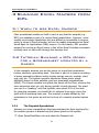
1 Introduction
1.1 Welcome to DPL 8 Enterprise
This DPL 8 Enterprise Manual is designed to supplement the DPL 8 Quick
Start Guide and DPL 8 Professional Manual that you received with your DPL
8 Enterprise software. This manual assumes you have significant
experience using DPL, and parts of it also assume familiarity with database
and programming concepts. This manual contains six chapters that cover
the features of DPL Enterprise.
If you are new to DPL, you should review the contents of the DPL
Professional Manual before proceeding to this manual. You may also wish
to complete the tutorials contained in those manuals. The DPL Professional
Manual also contains information on how to install DPL and how to get
help.
This manual is intended to be read while working with DPL. The chapters
of this manual are intended to be "stand-alone" and can be read in any
order.
A few conventions have been used in the text of the tutorial chapters. An
instruction to you in a tutorial will be contained in a bulleted paragraph
with an arrow, as follows:

Please do this step now.
Information to be entered in edit boxes, Excel cells, etc. is contained within
double-quotes. Do not include the double-quotes when entering the
information.
A brief outline of the contents of this manual follows.
Chapter 2 documents DPL Enterprise's database linking capabilities.
Throughout the chapter, you will complete a tutorial on how to set up and
run a database-linked model.
Chapter 3 illustrates how to link DPL Enterprise to a spreadsheet that
contains a calculation macro.
Chapter 4 covers DPL's expert aggregation interface and contains a tutorial
on how to create models with expert aggregation nodes in them.
1
Chapter 1: Introduction
Syncopation Software
Chapter 5 covers the Application Programming Interface (API). This feature
allows you to control and run DPL from other applications, such as Visual
Basic for Applications (VBA), C# and VB.NET.
Chapter 6 covers DPL's user function library interface.
2
Chapter 2: Database Linking in DPL
Syncopation Software
2 Database Linking in DPL
2.1 Overview
With DPL Enterprise you use data stored in a database to initialize nodes in
much the same way you can store data in Excel and use Excel initialization
links. In situations where some of the data you need for your DPL model is
already stored in a database and is subject to revision, using database
initialization links will ensure you have the most recent data and will reduce
errors due to data re-entry. In situations where multiple people need
access to the data and may be revising it, you can configure the database
to keep track of revisions.
This chapter discusses how to use database linking in DPL Enterprise.
2.2 ODBC Data Sources
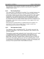
DPL communicates with a database via the Windows ODBC (Open
Database Connectivity) mechanism. See Figure 2-1.
Figure 2-1. DPL/Database Communication uses ODBC
By using ODBC, DPL gives you the flexibility to choose your database
management system or even change it as requirements evolve.
2.2.1
Setting up an ODBC Data Source for a Desktop Database
Before using database links in DPL, you must set up an ODBC data source
for the database with which you wish to communicate. You will do this now
for the example database delivered with DPL Enterprise. Depending on the
version of Windows you are running, the following steps for setting up the
data source may vary.
3
Chapter 2: Database Linking in DPL
Syncopation Software
DPL is presently a 32-bit program. If you are running DPL on a 64-bit
version of Windows, the 32-bit ODBC Datasource Administrator is in a
different location from the one specified below. If you follow the steps
below you will likely open the 64-bit Data Source Administrator, which will
not communicate with the example databases provided. You will need to
find the correct odbcad32.exe file and create a shortcut to it to set up the
Data source. For example, on the 64-bit version of Windows 7, the 32-bit
version of the Data Source Administrator is in
C:\Windows\SysWow64\odbcad32.exe. Oddly, the 64-bit (i.e., wrong)
version is in C:\Windows\System32\odbcad32.exe!




Open your Control Panel.
Click System and Security
Click Administrative Tools.
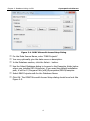
Double-click on Data Sources (ODBC). As mentioned above, be sure
you open the 32-bit Data Source Administrator. The ODBC Data Source
Administrator dialog appears. See Figure 2-2.
Figure 2-2. ODBC Data Source Administrator Dialog
4
Chapter 2: Database Linking in DPL
Syncopation Software
Among other things, the ODBC Data Source Administrator dialog displays
all the data sources currently configured on your computer. On the User
DSN tab, data sources that are available only to the logged in user are
displayed. On the System DSN tab, data sources available to all users of
the machine plus services are displayed.
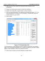
The ODBD Data Source Administrator dialog allows you to add new data
sources and delete or configure existing ones. You will now add a data
source.


Select the User DSN tab.
Click the Add button. The Create New Data Source dialog appears. See
Figure 2-3.
Figure 2-3. Create New Data Source Dialog

The sample database delivered with DPL Enterprise is a Microsoft
Access database. Select Microsoft Access Driver (*.mdb) from the list.

Click Finish. The ODBC Microsoft Access Setup dialog appears. See
Figure 2-4.
5
Chapter 2: Database Linking in DPL
Syncopation Software
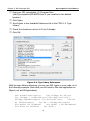
Figure 2-4. ODBC Microsoft Access Setup Dialog




For the Data Source Name, enter "R&D Projects".


Select R&D Projects.mdb for the Database Name.
You may optionally give the data source a description.
In the Database section, click the Select… button.
Use the Select Database dialog to browse to the Examples folder below
where you installed DPL Enterprise. If you used the default installation
path, it will be C:\Program Files (x86)\Syncopation\DPL8\Examples.
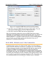
Click OK. The ODBC Microsoft Access Setup dialog should now look like
Figure 2-5.
6
Chapter 2: Database Linking in DPL
Syncopation Software
Figure 2-5. Completed ODBC Microsoft Access Setup Dialog

Click OK to close the ODBC Microsoft Access Setup dialog. The new
data source should appear in the User Data Sources list.

Click OK to close the ODBC Data Source Administrator.
Note: the information required to set up an ODBC Data Source varies
depending on the database to which the data source refers. For Access, the
only thing you had to specify was a file name and location. Access is a
desktop database. To configure a data source for a server-based database
such as Oracle, you will likely need to get information from your IT
department or database administrator.
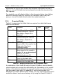
2.3 DPL Compliant Databases
A database that is going to be linked to DPL needs to have the tables or
queries that DPL will access structured in a particular way. If the database
is being developed primarily to store data that DPL will use, then you can
configure the tables in the database directly so that they meet the
requirements of DPL. If the database is pre-existing and/or will store data
for purposes other than for use with DPL, the tables within the database do
not need to be structured to be DPL compliant; rather queries and/or views
can be written to provide the necessary structure for DPL. Put another way,
the underlying tables can be structured in whatever way it is deemed
7
Chapter 2: Database Linking in DPL
Syncopation Software
appropriate as long as they contain the necessary information so that a
query or view of the table can be developed to provide the structure that
DPL requires.
For simplicity, we will refer to tables in the discussion below when talking
about the structure that DPL requires, but remember that it may be a
query or view of the table that provides the needed structure.
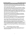
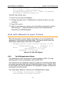
2.3.1
Required Fields
Table 2-1 summarizes the fields that are required in a table that stores
data DPL will access.
Field
Purpose
Type
Model ID
Identifies which model the
record belongs to. One of
this field or Project ID is
required.
Identifies which project the
record belongs to. One of
this field or Model ID is
required.
Identifies the specific data
item to DPL. It is used in the
Data tab of the Node
Definition dialog.
Tells DPL whether the data
item stored in the record is
scalar (0), a one-dimensional
array (1) or a twodimensional array (2).
Tells DPL the number of
rows for the data item.
Tells DPL the number of
columns for the data item.
Integer
Default
Name
ModelID
Integer
ProjectID
String
NodeID
Integer
Dims
Integer
Rows
Integer
Cols
Project ID
Node ID
Dimensions
Rows
Columns
Table 2-1. Required Fields for a DPL Compliant Table
A combination of the Model ID and/or Project ID fields is used to identify
which model and/or project the data belongs to. Depending on the overall
design of the decision and data management system you are developing,
you may want to use both. For example, if you are storing data in a
database for multiple different DPL models, you may want to identify which
model the data in each record belongs to by using the Model ID field. If
8
Chapter 2: Database Linking in DPL
Syncopation Software
you are developing a system in which multiple sets of data (e.g., each
associated with a specific project) will be used with a single DPL model,
you may want to use the Project ID field to identify these project data sets.
If the system will have both multiple models and multiple sets of data per
model, you may wish to use both fields.
A DPL compliant table needs to meet one more requirement. The fields in
each record that will store the data for each item must all begin with the
same prefix and must be numbered sequentially from 001 on. The default
data fields prefix is "Data_". A record that stores numeric information
should store the data for the data item in Data_001, Data_002, etc. You
may change the data fields prefix but the fields storing the data must end
with 001, 002, etc. For example, if your data fields prefix is "fld", then the
fields storing the data will be fld001, fld002, etc.
DPL can also access string data stored in a database. If a table stores
string data, then you must specify the String fields prefix. The default
prefix is "Str_". A record that stores string information should store the
data for the data item in Str_001, Str_002, etc.
Node IDs in a DPL compliant database cannot contain any punctuation or
spaces. They can contain letters or numbers but they must start with a
letter. Node IDs are case sensitive, i.e., "cost" is different from "Cost".
The order of the fields in each table does not have to match the order
shown in Table 2-1 above or Figure 2-6 below. However, the order in
which the data is stored within the data fields is important. If a record
contains a Node ID for a one-dimensional array with 3 elements, then the
data for the first element needs to be stored in the first data field
(Data_001 by default), the data for the second element needs to be stored
in the second data field (Data_002 by default), etc. Similarly if a record
contains a Node ID that is storing probabilities for a chance node, then the
probability for the first branch needs to be stored in the first data field, and
so forth.
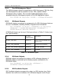
2.3.2
Required Fields for Revision Tracking
If you wish to set up a database that tracks revisions of data, then you
need to have two additional fields in a DPL compliant table. Table 2-2
summarizes these fields.
9
Chapter 2: Database Linking in DPL
Syncopation Software
Field
Purpose
Type
Default
Name
Revision
ID
Identifies which revision this
record is.
Integer
RevisionID
Revision
Date
The date the revision was
made.
Date
RevisionDate
Table 2-2. Required Revision Tracking Fields
The Revision ID field must be an integer greater than or equal to zero,
where a higher number indicates a more recent revision. For each table in
the database, every Model ID/Project ID/Node ID combination should have
an ascending set of Revision IDs without duplicates.
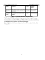
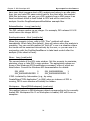
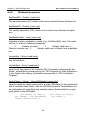
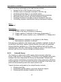
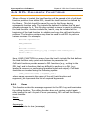
Figure 2-6 shows the Access design view for a DPL compliant table called
Project_Tbl.
10
Chapter 2: Database Linking in DPL
Syncopation Software
Figure 2-6. Access Design View of Project_Tbl
11
Chapter 2: Database Linking in DPL
Syncopation Software
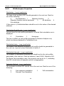
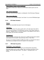
Figure 2-7 shows the Access datasheet view for Project_Tbl.
Figure 2-7. Access Datasheet View of Project_Tbl
12
Chapter 2: Database Linking in DPL
Syncopation Software
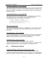
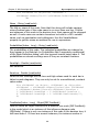
Figure 2-8 shows the Access design view for a DPL compliant table
containing string information called Project_Des.
Figure 2-8. Access Design View of Project_Des
13
Chapter 2: Database Linking in DPL
Syncopation Software
Figure 2-9 shows the Access database view for a DPL compliant table
containing string information called Project_Des.
Figure 2-9. Access Datasheet View of Project_Des
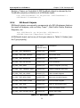
2.3.3
Table Names/Field Names
Table names and field names in a DPL compliant database cannot contain
any punctuation or spaces. They can contain letters or numbers but they
must start with a letter. Database management systems may vary
regarding whether table names and field names are case sensitive. To be
consistent with other identifiers in DPL, table names and field names are
case sensitive in DPL. Because a particular database management system
may or may not be case sensitive with regard to table and field names, you
cannot have table(field) names that differ only in case, e.g., both "field1"
and "Field1" are not allowed. The specific database management system
you are using may have other restrictions on table names and field names.
Please check with your database documentation.
14
Chapter 2: Database Linking in DPL
Syncopation Software
2.3.4
Scalar/Simple String Data
If you have a large number of scalar values and/or simple string values
(i.e., not arrays of strings) that DPL needs to access, these data can be
stored in a table that does not use the DPL compliant structure (i.e., having
Node ID, Dims, Rows, Cols) described above. These data may be stored in
tables in which the field/column names in the table identify the data, i.e., a
more standard database table structure. Tables not using the DPL
compliant structure must still have Model ID and/or Project ID fields as
appropriate and revision tracking fields as appropriate. Only scalar values
and simple string values can be stored in a table not using the DPL
compliant structure.
2.4 Configuring Database Access
within DPL
Once you have set up the database that you wish DPL to access, you need
to give DPL some database configuration information. You do this via the
Database Specification dialog. You must give this configuration information
to DPL before you can set up any database links within a model in DPL.
You will do this now.




Start DPL.
Select File | Open.
Navigate to the Examples folder underneath where you installed DPL.
If you used the default location, the path is C:\Program Files
(x86)\Syncopation\DPL8\Examples.
Select R&D Project No Links.da and click Open.
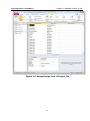
DPL opens the Workspace as shown in Figure 2-10.
15
Chapter 2: Database Linking in DPL
Syncopation Software
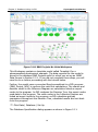
Figure 2-10. R&D Projects No Links Workspace
This Workspace contains a template model called Template1 for a
pharmaceutical development example. The data required for the model is
stored in the database R&D Projects.mdb for which you set up an ODBC
Data Source in Section 2.2.1. If you did not complete those steps, you will
need to do so before proceeding with the tutorial below.
Further, the model uses a converted Excel spreadsheet in a DPL program
(R&D_Project_NPV) to perform the cash flow calculations. The chance and
decision nodes in the Influence Diagram are calculation linked as export
nodes to the program. As DPL analyzes the Decision Tree, the export nodes
send data to the program. The value nodes in the Influence Diagram are
linked as import nodes to the program; as DPL calculates get/pay
expressions throughout the Decision Tree, calculated results are sent back
from the program.

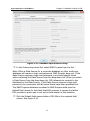
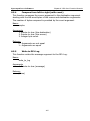
Click Data | Database | Set Up
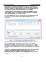
The Database Specification dialog appears as shown in Figure 2-11.
16
Chapter 2: Database Linking in DPL
Syncopation Software
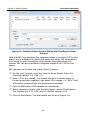
Figure 2-11. Database Specification Dialog

In the Source drop-down list, select R&D Projects from the list.
Note: Often a Data Source for a corporate database or other multi-user
database will require a login and password. R&D Projects does not. If the
Data Source requires a login and password, you should specify those
before selecting the Data Source from the drop-down list. When you select
a Data Source from the drop-down list, DPL attempts to connect to the
database for the Data Source. If the Data Source requires a login and
password, the connection will fail unless these have been provided first.
The R&D Projects database contained in R&D Projects.mdb uses the
default field names for the fields that DPL requires to access the tables.
DPL provides a quick way to set up the field names in this situation.

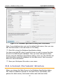
Click the Default field names button. DPL fills in the required field
names. See Figure 2-12.
17
Chapter 2: Database Linking in DPL
Syncopation Software
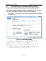
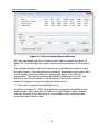
Figure 2-12. Database Specification Dialog with Field Names
Note: if your database does not use the default field names, then you may
edit the field names in the edit boxes on the dialog.

Click OK to close the Database Specification dialog.
You have now told DPL what it needs to know in order to access the data
stored in the R&D Projects database. Since you have changed the Data
Source using the Database Specification dialog, when you click OK DPL will
load information about the database for the data source. See the section
below for more information.

Save your Workspace file under a new name.
2.5 Loading Database Schema
When you change the Data Source in the Database Specification dialog,
DPL loads the database schema for the Data Source. Specifically, DPL
gathers the table names, field names within each table and other
18
Chapter 2: Database Linking in DPL
Syncopation Software
information about the database. For a database that is on a remote server
or is sizeable, it may take a few minutes to load this information and you
may notice a delay. DPL uses this information in a number of places. This
information only needs to be loaded once (and only needs to be re-loaded
if the structure of the database has changed, e.g., if new tables have been
added, or new fields to tables). The schema information is saved with the
DPL Workspace file when you save it.
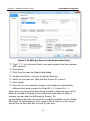
If you know the structure of the database has changed, you may ask DPL
to load database schema by going to Data | Database | Load Schema.
Further, when you first set up a DPL Workspace file with a Data Source
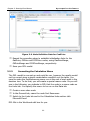
specified, DPL will prompt you as to whether you wish to load database
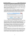
information each time the Workspace is opened. See Figure 2-13.
Figure 2-13. Load Database Information Prompt
During the development phase of the database, the structure may change
and you may wish to answer Yes to this question and check the "Don't ask
this question again" checkbox. DPL will then automatically load the
database schema each time the Workspace is opened. Alternatively, if you
don't check the checkbox, you will be asked each time the Workspace is
loaded. Leaving the checkbox unchecked may be wise for large and/or
remote databases, particularly if you work offline and might not have
access to the database. Once you have finalized the design of the
database, you no longer need to regularly load the schema. At this point, it
makes sense to change the setting to "Don't load" via File | Options |
Workspace.
Lastly, as indicated above, the information that DPL gathers when loading
the database schema is structural in nature. DPL is not loading the actual
data stored in the tables when it loads the schema information. DPL does
the data extraction from the database when you run a database-linked
model or when you create a program from a database-linked model.
19
Chapter 2: Database Linking in DPL
Syncopation Software
2.6 Creating Database-Linked
Models
In order to create a database-linked model, you must first set up the Data
Source using the Database Specification dialog via Data | Database | Set
Up. This is explained in Section 2.4. If you have not already completed the
tutorial in that section, please do so now.

If it is not already open, browse to find the file that you saved from
Section 2.4 and open it now.

If the Load Database Information prompt comes up, select No and
check "Don't ask this again".
2.6.1
Linking Existing Nodes to a Database
The file that you started with in Section 2.4 contains a number of nodes
that are missing node data and that are ready to be linked to the database.
This section will show you how to add database links to an existing node.
Before you do this, you will explore the database R&D Projects database. If
you do not have Access on your computer, you will not be able to explore
the database but you may wish to read through this section and explore
the figures.

If you have Access on your computer, use Windows Explorer to
Navigate to the Examples folder underneath where you installed DPL.
If you used the default location, the path is C:\Program Files
(x86)\Syncopation\DPL8\Examples.

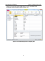
Double-click on R&D Projects.mdb to open it in Access. See Figure
2-14.
20
Chapter 2: Database Linking in DPL
Syncopation Software
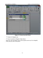
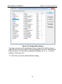
Figure 2-14. R&D Projects Database Open in Access

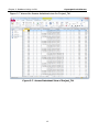
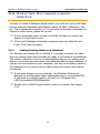
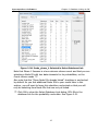
In the Navigation pane on the left, double-click on Project_Tbl to open
it in datasheet view. See Figure 2-15.
21
Chapter 2: Database Linking in DPL
Syncopation Software
Figure 2-15. Project_Tbl Open in Datasheet View
Note that there are a number of datasets in the table. Specifically there are
records with Node IDs for six projects which are identified by Model ID = 1
(all of them have the same Model ID) and Project IDs 1 through 6. This
database is also configured for revision tracking (this will be covered in
Section 2.7), so each Model ID and Project ID combination has a number
of revisions for each Node ID. For example, the first five rows of the table
all store different revisions for the Node ID probs_phase_1. Note: the data
may be the same for each of the revisions.


Explore the table some more if you'd like.
Do not make any edits to the data.
If you are unfamiliar with Access, you should know that any edits you make
are instantly saved. You are not prompted to save changes when you close
Access; the edits are automatically saved as you make them.
Note in particular that there is a project with Model ID = 1 and Project ID
= 1. You will use this in DPL.
22
Chapter 2: Database Linking in DPL
Syncopation Software



Close Access.
Switch back to DPL.
Double-click on the Phase 1 success node in the Influence Diagram.
Note that the node has no probability data. See Figure 2-16.
Figure 2-16. Node Definition Dialog for Phase 1 Success
As you may have noticed while exploring the database, the probability data
for this node as well as the other chance nodes in the model are stored in
the database in a table called Project_Tbl.


Switch to the Links tab.
In the Initialization Links section, select Database.
Note: database links are always initialization links. I.e., DPL will get the
data for the node from the database once at the beginning of a run. The
data is then used in the subsequent analysis.
When setting up a database link for a node, you must tell DPL the Model
ID and/or Project ID of the record you wish to link to. This is also done in
the Initialization Links section, and DPL displays the Model ID and Project
ID edit boxes on the Links tab when Database is selected as the
Initialization Link type.

Type 1 in the Model ID exit box.
23
Chapter 2: Database Linking in DPL

Syncopation Software
Type 1 in the Project ID edit box. Note: this is the project that you saw
when you browsed the database table. The Links tab should now look
like Figure 2-17.
Figure 2-17. Completed Links Tab for Phase 1 Success

Switch back to the Data tab. Note: that there is now a Link button
(
) next to the probability and value edit boxes. See Figure 2-18.
24
Chapter 2: Database Linking in DPL
Syncopation Software
Figure 2-18. Data Tab with Link Button
The Link button allows you to tell DPL the table and Node ID that the node
is linked to via the Select Database Link dialog.

Click the Link button (
2-19.
) next to the probability edit box. See Figure
25
Chapter 2: Database Linking in DPL
Syncopation Software
Figure 2-19. Select Database Link Dialog
The Select Database Link dialog provides a combo box at the top for you to
select the table in the database for the link. When you select a table, the
list below the combo box is populated with the Node IDs within that table.
Currently, the table selected is Name_Tbl (this is a descriptive table with
string data in it; you will not be using this table).

Use the drop-down list to select Project_Tbl.
The list of Node IDs also contains information about the data for each
Node ID. The list tells you the total count of data elements for the item,
the dimensions, rows and columns.

In the list below, select probs_phase_1 as the Node ID. See Figure
2-20.
26
Chapter 2: Database Linking in DPL
Syncopation Software
Figure 2-20. Probs_phase_1 Selected in Select Database Link
Note that Phase 1 Success is a two-outcome chance event and that you are
selecting a Node ID with two data elements for its probabilities, so the
Count column reads "2".
Also note that the "Show Node IDs already linked" checkbox is unchecked
by default. As you link additional Node IDs to your model later in this
section, you will want to leave this checkbox unchecked so that you will
only be selecting from Node IDs that are not yet linked.

Click OK to close the Select Database Link dialog. DPL fills in the
database link for the probability node data. See Figure 2-21.
27
Chapter 2: Database Linking in DPL
Syncopation Software
Figure 2-21. Database Link Node Data for Phase 1 Success
The syntax for the database link node data is as follows.
=[Project_Tbl.NodeID]=probs_phase_1[2]
The node data must start with "=[" to indicate a database link. The
information contained within the square brackets is of the form
table_name.NodeID which indicates to DPL which table the Node ID is in,
e.g., Project_Tbl. Immediately following the closed square bracket is
another equal sign. Following this second equal sign is the Node ID that
the node is linked to, e.g., probs_phase_1. The information following the
Node ID tells DPL the dimensionality of the data, i.e., this is a two column
row array. For more information on arrays within DPL, see Chapters 9 and
15 of the DPL Professional Manual.
As with Excel initialization links, when you use a database initialization link,
the link only appears on the first branch of the node (for Phase 1 Success
this is the Yes branch). In this example, you are using a database
initialization link for the probability data. Therefore, the remaining
probability data for the node must be blank. The same applies for value
data. The initialization link appears on the first branch and all remaining
value data must be blank.
DPL will only allow you to put an initialization link on the first branch.

Press the down arrow key twice to move the selection to the
probability data for the No branch.
28
Chapter 2: Database Linking in DPL
Syncopation Software
Note that the Link buttons for both the probability data and the value data
are now disabled.

Click OK to close the Node Definition dialog.
You have now specified a database link for the Phase 1 Success node.
Note: the value data for the node (1, 0) is not stored in the database.



Double-click Phase 2 success to edit its definition.
Switch to the Links tab.
Select Database in the Initialization Links section.
Note that DPL fills in the Model ID and Project ID that you used previously.
You can have database links to multiple Model ID/Project ID records within
a model, though in most cases this won't be necessary. DPL assumes you
want to use the same Model ID/Project ID as the existing link(s).

Switch to the Data tab.

Click the Link ( ) button. The Select Database Link dialog appears.
This time it has Project_Tbl already selected since that is the last table
you used.


Select probs_phase_2 in the list.

Click OK to close the Node Definition dialog.
Click OK to close the Select Database Link dialog. Again, DPL fills in the
database link for the Yes branch of the node and leaves the No branch
blank.
Repeat the above procedure to create database initialization links for the
probabilities of the remaining chance nodes in the model using the Node ID
for each node as indicated in Table 2-3. You may need to delete probability
data from some of the nodes. As mentioned earlier, leave the Show Node
IDs already linked checkbox unchecked, so that after you link a Node ID it
will not appear in the list the next time you use the dialog.
29
Chapter 2: Database Linking in DPL
Syncopation Software
Node
Node ID
Phase 3 success
probs_phase_3
Regulatory approval
probs_regulatory_approval
Market size
probs_market_size
Market share
probs_market_share
Pricing
probs_pricing
Strength of competition
probs_strength_of_competition
Table 2-3. Node IDs for Probability Database Initialization Links

Save your file.
When you created the database initialization link for the Market share
node, you may have noted that the syntax for the database initialization
link for it is:
=[Project_Tbl.NodeID]=probs_market_share[3][3]
The Node ID for the market share probabilities is a two-dimensional array.
Market share is conditioned by Strength of competition. Both Market share
and Strength of competition are three-outcome chance nodes. Therefore,
nine probabilities are needed for Market share and these are stored in a 3
by 3 array. DPL indicates this dimensionality in the database initialization
link by adding "[3][3]" following the Node ID.
The Pricing node is also conditioned and also uses a two-dimensional (3 by
3) array link.
The model is now ready to run.

Press F10 to run a decision analysis.
DPL extracts the data for the probabilities for each chance node from the
database and produces the requested results.
30
Chapter 2: Database Linking in DPL
Syncopation Software
2.6.2
Changing Records for Database Initialization Links
The Model Links dialog displays all the records (Model ID, Project ID
combinations) that the model is linked to. In this dialog you can also
change records that the model is linked to. You will do this now in order to
see results for a different project in the R&D Projects database.

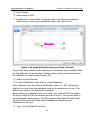
Click Model | Links | Options. The Model Links dialog appears as shown
in Figure 2-22.
Figure 2-22. Model Links Dialog
This model is currently linked to one record (Model ID/Project ID
combination), namely Model ID = 1 and Project ID = 1.


Select the record in the first row of the Database Links list box.
Press F2 to edit the record. Note that the record changes to two
comma separated numbers. See Figure 2-23.
31
Chapter 2: Database Linking in DPL
Syncopation Software
Figure 2-23. Editing a Record in the Model Links Dialog

Type "1, 2" for the record. Note: you must separate the two numbers
with a comma.






Press Enter.
Click Close to close the Model Links dialog.
Double-click Phase 1 success to edit its definition.
Switch to the Links tab. Note that the Project ID is now 2.
Click Cancel.
Press F10 to run a Decision Analysis. The results are substantially
different from what you got for Model ID = 1, Project ID = 1.
Note: when you change the record that a model is linked to, none of the
tables it is linked to change. If you look at the node data for Phase 1
success, you can see it is still linked to Project_Tbl.
As mentioned previously, you can link a model to multiple records (Model
ID/Project ID combinations). If you wish to link a node to a new record,
you do this via the Links tab. You will try this now.
32
Chapter 2: Database Linking in DPL
Syncopation Software

In the influence diagram, double-click Phase 1 success to edit its
definition.



Switch to the Links tab.
Set Project ID to be 1.
Click OK. You will get the prompt shown in Figure 2-24.
Figure 2-24. Change Record Prompt

Answer No to the prompt.
By answering no, you are telling DPL not to change any other nodes linked
to record Model ID = 1, Project ID = 2. Phase 1 success will now be linked
to Model ID = 1, Project ID = 1, while the remaining chance nodes are
linked to Model ID = 1, Project ID = 2. Therefore, the probability of
success for phase 1 is from project 1 in the database, while the rest of the
probabilities are from project 2.






Go to Model | Links | Options to see this.
Click Close.
Press F10 to run a decision analysis. The results are different yet again.
Go to Model | Links | Options again.
Restore your model to only be linked to Model ID = 1, Project ID = 2
by editing the record for Model ID = 1, Project ID = 1 to be 1, 2. DPL
updates the linked records in the model.
Click Close.
33
Chapter 2: Database Linking in DPL
2.6.3
Syncopation Software
Creating New Database-Linked Nodes
You may have noticed that there are a number of costs and other
assumptions associated with each R&D project stored in the R&D Projects
database. When evaluating each project in the database, you would want
to take into account these project specific assumptions. As the model
currently stands, when you changed from analyzing Project ID = 1 to
Project ID = 2, the costs and other assumptions did not change. You will
correct this now.
To see the costs and other assumptions that are currently being used, you
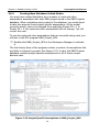
will look in the DPL program R&D_Project_NPV.

Double-click R&D_Project_NPV in the Workspace Manager to activate
it.
The first twenty lines of the program contain a number of assumptions that
are likely to change by project. See Figure 2-25. In fact, the R&D Projects
database contains project specific assumptions for all of these except
discount rate.
Figure 2-25. Project Specific Assumptions in R&D_Project_NPV
34
Chapter 2: Database Linking in DPL
Syncopation Software
You will create database linked value nodes for these project specific
assumptions.


Double-click Template1 in the Workspace manager to activate it.
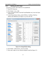
Drop-down the Model | Links | Add split button and choose Database
Initialization-Linked... from the list. The Create Database Linked Values
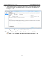
dialog comes up as shown in Figure 2-26.
Figure 2-26. Create Database Linked Values Dialog
This dialog allows you to select one or more Node IDs from one or more
tables in the database that the DPL Workspace is connected to, and create
database-linked value nodes for each. It displays similar information to the
information in the Select Database Link dialog. In addition, you can tell DPL
whether to prefix node names with the table name, whether to create
arrays based on the dimensions of the data in the database, and whether
to create DPL export nodes.

If Project_Tbl is not selected in the combo box, select it.
35
Chapter 2: Database Linking in DPL
Syncopation Software

Make sure the Show Node IDs already linked checkbox is still
unchecked.



Check the Create arrays based on data size checkbox.

Check the Create DPL program export nodes checkbox.
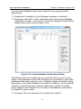
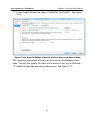
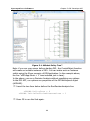
Click the Select All button. The dialog should look like Figure 2-27. You
have selected all the Node IDs in the Project_Tbl table that were not
already linked to your model.
Click Create.
Figure 2-27. Selected Node IDs
If you needed to create database-linked nodes for Node IDs from another
table, you could select that table now, select the Node IDs and click Create
again. In this example, you do not need to do that.

Click Close to close the Create Database Linked Values.
36
Chapter 2: Database Linking in DPL
Syncopation Software

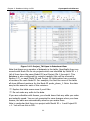
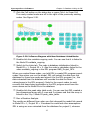
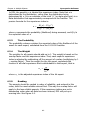
Click the Full button on the status bar or press Ctrl+L to Zoom Full.
The newly created nodes are off to the right of the previously existing
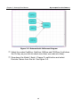
nodes. See Figure 2-28.
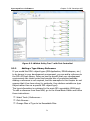
Figure 2-28. Influence Diagram with New Database-Linked Nodes

Double-click the costdata ongoing node. You can see that it is linked to
the Node ID costdata_ongoing.

Switch to the Links tab. The node is database initialization linked to
Model ID = 1, Project ID = 2. Also the node is calculation linked to the
value costdata_ongoing in the DPL program R&D_Project_NPV.
When you created these nodes, you told DPL to create DPL program export
nodes. Now when you run the model, DPL will extract the data from the
database for these new nodes and export it to the DPL program (i.e., the
data extracted from the database will override the data for these
values/arrays in the DPL program). Note for the export nodes to work
correctly the items being overridden in the DPL program must have the
same names as the Node IDs in the database.

Double-click the peak sales table node. You can see that DPL created a
two-dimensional array with 3 rows and 3 columns and that the array is
linked to the 3 by 3 Node ID peak_sales_table.

Run a Decision Analysis.
The results are different from when you first changed the model link record
to Model ID = 1, Project ID = 2 because the costs and other assumptions
DPL is using are now extracted from the database for project 2, whereas
37
Chapter 2: Database Linking in DPL
Syncopation Software
previously DPL was using the assumptions in the DPL program which differ
from what is in the database for project 2.
2.6.4
Node Data Syntax for Non-DPL Compliant Tables
As mentioned in Section 2.3.4, you may store scalar and simple string data
in a non-DPL compliant table. The syntax for the database link node data is
slightly different in this case. The syntax is as follows
=[Project_Info.InPortfolio]
As with nodes linked to tables containing Node IDs, the node data must
start with "=[" to indicate a database link. In this case though, the
information contained within the square brackets is of the form
table_name.field_name which indicates to DPL which table the data is in,
e.g., Project_Info and which field the data is in, e.g., InPortfolio. Nothing
follows the closed square bracket. No dimensionality information is needed
since the node must be a scalar or simple string.
You may use same the methods described in Sections 2.6.1 and 2.6.3 to
link existing nodes and create new database linked nodes to non-DPL
compliant tables for scalars and simple strings.
2.7 Databases Configured for
Revision Tracking
One reason to store data in a database is to keep track of the various
revisions that the data may go through while the project or asset is being
analyzed.
If you have set up your database so that it tracks revisions, you must tell
DPL this and provide it with some more information about the field names
in the database. You do this in the Database Specification Dialog. For
databases that are configured for revision tracking, both a Revision ID and
Revision Date field must exist in each table storing project data.


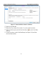
Click Data | Database | Set Up.

Click Default field names to set the field names for the two revision
fields.

Click OK.
Check the Database configured for revision tracking checkbox. The
Revision ID and Revision Date field edit boxes are enabled.
38
Chapter 2: Database Linking in DPL
Syncopation Software
The R&D Projects database was already configured for revision tracking,
although you have not been using it as such up to this point. Therefore,
you did not have to change the Source or change the database in any way.
Normally you would probably set the Database is configured for revision
tracking at the same time as initially specifying the data source and DPL
would automatically load the database schema information. In this case
you have not changed the data source and DPL did not automatically load
the database schema, so you need to do it now.



Select Data | Database | Load Schema. Click Yes for the prompt.
Save the Workspace.
Run a Decision Analysis.
Note that the results are slightly different. Previously when DPL did not
know the database was configured for revision tracking, it was using the
first data set it found for Model ID = 1, Project ID = 2. Now that DPL
knows the database is configured for revision tracking, it uses the most
recent revision which is slightly different.
39
Chapter 2: Database Linking in DPL
Syncopation Software
40
Chapter 3: Running Excel Macros
Syncopation Software
3 Running Excel Macros from
DPL
3.1 When to Use Excel Macros
Most spreadsheet models are built in such a way that the outputs (e.g.,
NPV) are updated as part of a normal Excel recalculation. However, some
models may include calculations that are difficult or impossible to express
solely in terms of Excel formulas, but can be readily programmed as Excel
Visual Basic for Applications (VBA) macros. For this reason, DPL provides
support for running an Excel macro in lieu of the Excel Calculate command
normally sent on each path through the decision tree.
3.2 Tutorial: Building a DPL Model
for a Spreadsheet Updated by a
Macro
In this example, assume you are the owner of a gas-fired combustion
turbine electricity generating plant. The plant is part of a system consisting
of many generating stations using various energy sources: nuclear, wind,
coal, gas, etc. The system operator dispatches these power plants
efficiently based on their variable costs per generated megawatthour
(MWh). The lowest variable cost plants run nearly all the time, whereas the
more expensive ones run only during periods of peak demand. The plant
you own is a "peaking" unit that typically runs about 20% of the time.
For planning purposes, you would like to estimate how many hours the
plant will be operating next year. The problem is made difficult by the
uncertainty in fuel prices as well as the level of a recently enacted carbon
tax.
3.2.1
The Dispatch Spreadsheet
Assume you have a spreadsheet that approximates the logic employed by
the system operator in dispatching the power plants in the system.

Open PowerPlantMacro.xls and select the Dispatch tab.
41
Chapter 3: Running Excel Macros
Syncopation Software
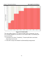
Figure 3-1. Power Plant Dispatch Sheet
Under base case assumptions, the plant falls in the bottom half of the
dispatch order and runs about 19% of the time (cell C22). The units
immediately ahead of the plant are old, less efficient coal-fired plants. A
high carbon tax might mean that your plant runs more, since it would push
up the costs of plants currently above yours more than your costs.


Select the DPL tab.
Change the green CO2 Price cell to 150.
42
Chapter 3: Running Excel Macros
Syncopation Software
Figure 3-2. Power Plant DPL Sheet


Select the Dispatch tab.
Press the Refresh Dispatch Order button.
Note that with the higher carbon tax the plant moves up in the dispatch
order and runs 34% of the time.
43
Chapter 3: Running Excel Macros
Syncopation Software
Figure 3-3. Power Plant Dispatch Sheet Updated
The Refresh Dispatch Order button runs a macro that sorts the power
plants by their variable costs to update the dispatch order.

Click Developer | Code | Visual Basic. If the Developer tab isn’t visible
in the Excel Command Ribbon go to File | Options | Customize Ribbon
and click the checkbox next to Developer in the Customize the Ribbon
section on the right.

Once Visual Basic is open, in the left-hand pane, double click on
Module1.
The SortResources() macro is displayed in the Visual Basic Editor.


Sub SortResources()
Calculate
Worksheets("Dispatch").Activate
Names("ResourcesTable").RefersToRange.Select
Selection.Sort
Key1:=Names("DispCost").RefersToRange
CalculateEnd Sub
Close the Visual Basic Editor.
Select the DPL tab and change CO2 Price back to 50.
44
Chapter 3: Running Excel Macros
Syncopation Software
3.2.2
Building the DPL Model
You will now create a DPL Model for the spreadsheet.



Start DPL Enterprise.

In the Range Names dialog, select CO2Price, CoalPrice, GasPrice,
OilPrice and Utilization (see Figure 3-4), then click OK.
Click Model | Links | Add.
Press the Browse button and find PowerPlantMacro.xls, then click Open
and then OK.
Figure 3-4. Range Names Dialog


Click Model | Influence/Arc | From Formulas.
Move your nodes so your influence diagram looks like Figure 3-5.
45
Chapter 3: Running Excel Macros
Syncopation Software
Figure 3-5. Deterministic Influence Diagram

Select the nodes CoalPrice, GasPrice, OilPrice and CO2Price (hold down
the Ctrl key as you click to select more than one node at a time).

Drop-down the Model | Node | Change To split button and select
Discrete Chance from the list. See Figure 3-6.
46
Chapter 3: Running Excel Macros
Syncopation Software
Figure 3-6. Probabilistic Influence Diagram
You now need to provide data for the chance nodes. The Assumptions
sheet in the spreadsheet has Low-Nominal-High ranges for each of them.
You'll use Initialization Links to tell DPL to use the range data in the
spreadsheet.


Double-click on CoalPrice to bring up the Node Definition dialog.
Switch to the Links tab and in the Initialization links section click
Microsoft Excel. See Figure 3-7.
47
Chapter 3: Running Excel Macros
Syncopation Software
Figure 3-7. Node Definition Links for CoalPrice


Switch to the Data tab.

Select the first branch and click the link button (
edit box.

In the first column, select CoalPriceRange (see Figure 3-8) and then
click the Select button.
Delete the three values (the number 2 on each of the branches).
48
) next to the Value
Chapter 3: Running Excel Macros
Syncopation Software
Figure 3-8. Range Names Dialog
You have now set up the initialization links so that the CoalPrice chance
node will use the three values in the spreadsheet for its Low, Nominal and
High branches. You will use the default probabilities of .3, .4, .3 for this
example. See Figure 3-9.

Click OK to close the Node Definition dialog.
49
Chapter 3: Running Excel Macros
Syncopation Software
Figure 3-9. Node Definition Data for CoalPrice

Repeat the preceding steps to establish initialization links for the
GasPrice, OilPrice and CO2Price nodes, using GasPriceRange,
OilPriceRange and CO2PriceRange, respectively.

Save your DPL model.
3.2.3
Connecting the Calculation Macro
The DPL model is now set up and could be run, however the results would
not be correct since a simple recalculation wouldn't sort the table. You
need to make the SortResources macro run at the end of each path in the
decision tree. To do that, you will create a special macro node. As you will
see in the following, you indicate to DPL that the node is a macro node on
the Links tab. You specify the macro to be run on the Data tab.



Create a new value node.
In the General tab, name the node Sort Resources.
Switch to the Links tab and in the Calculation links section click
Microsoft Excel.
DPL fills in the Workbook edit box for you.
50
Chapter 3: Running Excel Macros
Syncopation Software

In the Sheet/Cell edit box, type in "XLMACRO.CALCULATE". See Figure
3-10.
Figure 3-10. Node Definition Links for the Sort Resources Macro Node
DPL recognizes the special cell name as the code for a calculation macro
node. You will now specify the name of the macro to run on the Data tab.

Select the Data tab and type SortResources. See Figure 3-11.
51
Chapter 3: Running Excel Macros
Syncopation Software
Figure 3-11. Node Definition Data for the Sort Resources Macro Node
SortResources is the name of the update macro.
Note: Calculation macros must be VBA Subs without any parameters. If you
need to pass parameters to your macro, just add one or more DPL Export
nodes and have the macro check the values of the cells to which those
nodes are linked. The macro name is case sensitive.

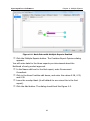
Click OK to close the Node Definition dialog. Your model should now
look similar to Figure 3-12.
52
Chapter 3: Running Excel Macros
Syncopation Software
Figure 3-12. Influence Diagram with Sort Resources Macro Node
You are now ready to run the model.

In the Home | Run group, make sure Risk Profile is checked and
uncheck Policy Tree.

Click Home | Run | Decision Analysis.
53
Chapter 3: Running Excel Macros
Syncopation Software
Figure 3-13. Risk Profile
The risk profile in Figure 3-13 shows a broad range of outcomes. You can
run a tornado diagram to see which of the chance nodes is contributing the
most uncertainty.

Drop-down the Home | Sensitivity | Tornado split button and select
Base Case from the list.

Click OK to accept the default Low/Nominal/High assignments.
54
Chapter 3: Running Excel Macros
Syncopation Software
Figure 3-14. Tornado Diagram
Figure 3-14 indicates that GasPrice is the most sensitive variable, which is
what you expect since you're running a gas-fired plant, but CO2 and Oil
prices are also significant. Coal price is not sensitive. As it is modeled, the
risk in the dispatch cost of a coal plant is primarily driven by CO2
emissions.
55
Chapter 3: Running Excel Macros
Syncopation Software
56
Chapter 4: Multiple Experts
Syncopation Software
4 Multiple Experts
4.1 Why Use Multiple Experts?
Decision analysis requires the assessment of probability distributions using
data, expert judgment, or most often, a combination of these. Probability
distributions are defined by the DPL analyst, but to acquire the necessary
knowledge and/or data, the analyst often needs to consult experts, and
different experts often have different opinions. For chance nodes with two
states (also known as binomial chance events), DPL provides a built-in
capability to aggregate probability assessments from several experts. This
chapter explains and demonstrates how this multiple experts feature
works.
For purposes of this chapter, the quantity being assessed (a probability of a
particular event occurring) will be called a likelihood to avoid confusion
with the other probabilities involved in the calculations.
Probability assessments are often difficult, and experts may have
significantly differing views. Given a variety of experts and their
assessments, the analyst would like to come up with some sort of weighted
average likelihood to use in the analysis. One possibility is to simply apply
weights to each expert and compute a straightforward weighted average.
However, this method does not directly incorporate any measure of the
degree of confidence in each expert's assessment. It also does not capture
the overlap of knowledge across experts.
DPL's aggregation method uses data provided by the analyst to calculate
the weights and the overall expected likelihood. The weights used by DPL
are determined by the reliability of the expert (measured by the
assessments the expert provides) and the amount of shared information
among the experts (measured by an overlap factor). DPL's method is
simple and quick to use.
4.2 Overview of DPL's Multiple
Experts Feature
Through a process of careful questioning, a distribution of likelihoods is
extracted from each expert. To use DPL's multiple experts feature, each
57
Chapter 4: Multiple Experts
Syncopation Software
expert must provide his/her assessment of the 10th, 50th, and 90th
percentiles for the likelihood in question. The analyst ranks the experts
from most "reliable" to least, and enters the 10-50-90 percentile values
(referred to as fractiles) from the distribution for each expert.
An overlap factor is also required for all experts entered after the first
(most reliable) expert. This quantity represents the amount of shared
information the experts are believed to have.
DPL approximates each expert's distribution as a Beta distribution, and
computes an expected value of the weighted average of all the
distributions.
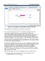
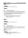
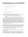
Figure 4-1. DPL Dialog for Combining Expert Opinions
Look at the top row of the Combine Expert Opinions dialog in Figure 4-1.
The following headings appear: Name, 10%, 50%, 90%, Overlap,
Experience, Probability, and Weight. Each of these is a quantity used to
calculate the overall likelihood of the event. The fractiles and overlap
factors are entered by the analyst, and the other quantities are calculated
by DPL.
In Figure 4-1, a highly experienced expert and a less experienced expert
have each assessed likelihoods for an uncertain event. The less
experienced expert has provided a wider range around his or her 50%
(median) point estimate. The combined probability for the two experts is
0.4875.
58
Chapter 4: Multiple Experts
Syncopation Software
The subsections below provide descriptions of each quantity in this dialog.
The last section of this chapter provides a brief tutorial on using DPL's
Multiple Experts feature.
4.2.1
The Overlap Factor
The overlap factor is provided by the analyst. It is a number between zero
and one, representing the fraction of the information provided by that
expert that overlaps the information already represented by other experts.
For example, if two academic experts are entered who are in the same
department, have read the same books, and have attended the same
seminars, the second one entered may have an overlap factor close to 1.
An overlap factor of zero implies that the expert with zero overlap has only
information or data that is entirely unknown to other experts; this is not
typically the case.
Determining the overlap factors is a challenge left to the analyst. It is
important to consider using overlap factors in order to avoid overrepresenting any one source of information.
4.2.2
The Experience Index
The experience index is calculated by DPL. This number represents the
amount of information in each expert's assessment, and is based on the
10-50-90 fractiles.
This quantity is most easily explained by the "colored balls in an urn" model
of the Beta distribution. Suppose the quantity being assessed is the
probability that you will pick a red ball from an urn with an unknown
percentage of red balls. An expert draws n balls from the urn, where n is
different for each expert. Based on the size of the sample drawn (n) and
the portion of the balls drawn that are red, the expert constructs his or her
own distribution of the likelihood of drawing a red ball. As n increases, the
accuracy of the expected value of the likelihood increases.
59
Chapter 4: Multiple Experts
Syncopation Software
In DPL, the quantity n is labeled the experience index. Note that n is
determined by the distribution, rather than the distribution being
determined by n. It is an estimate of the total "n" (or alpha plus beta) in a
Beta distribution that approximately corresponds to the fractiles. The
precise formula for the experience index is:
E ( p) − E ( p 2 )
n=
E ( p 2 ) − ( E ( p )) 2
where p represents the probability (likelihood) being assessed, and E(x) is
the expected value of x.
4.2.3
The Probability
The probability column contains the expected value of the likelihood of the
event for each expert, calculated from the 10-50-90 fractiles.
4.2.4
The Weight
The weights for all experts should add up to 1. The weight is based on the
overlap factor and the experience index. First, each expert's experience
index is adjusted by subtracting off the amount of overlap (multiplying by 1
– overlap factor). Then the weight for the kth expert represents the
fraction of all total experience that is attributable to that expert, that is:
wk =
nk
∑ ni
where ni is the adjusted experience index of the ith expert.
4.2.5
Ranking
The experts should be ranked in order of reliability, and entered in this
order, with the most reliable entered first. This way the overlap factor will
apply to the less reliable experts. If the experience indices are not in
descending order when all data has been entered, DPL will put up a
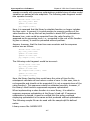
warning box. See Figure 4-2.
60
Chapter 4: Multiple Experts
Syncopation Software
Figure 4-2. DPL Warning About Expert Rankings
In general, more reliable experts should have higher experience indices.
DPL is checking to make sure the entries are what you intended.
If an expert believed by the analyst to be less experienced has a very high
experience index, it may be that this expert is not well calibrated and has
provided 10-50-90 fractiles that are closer together than they should be
given his/her knowledge. The analyst must exercise judgement to ensure
that the opinion of an overconfident expert is not overweighted.
4.3 Tutorial: Using Multiple Experts
to Assess Early Product
Approval
Suppose you are a decision analyst at a firm that is preparing to launch an
exciting new product early next year. Plans are in place for an expensive
product launch, including millions of dollars in advertising and promotions
and a large kickoff meeting for the global sales team. Government
regulators were on track to approve the product at the end of the calendar
year, so the product launch has long been scheduled for the first quarter of
the next year. You've done an extensive DPL analysis of decisions
surrounding the product launch, but the launch timing was never in
question.
You just received a call with new information. Because of the national
election in November, there are rumors that the regulators in your industry
are going to speed up approvals during the summer and fall, which could
lead to your product being approved and launched a few months early
(i.e., only a few months from now). If this happens, the promotional events
and other pre-launch investments may need to be accelerated at significant
61
Chapter 4: Multiple Experts
Syncopation Software
cost. You need to adjust your DPL analyses accordingly, and the NPV of the
product will change.
You decide to consult a few external and internal experts to better
understand the likelihood that the product will be approved (and launched)
in the current calendar year, so that you can incorporate this new
uncertainty into your models.





Start DPL 8 Enterprise (if it isn't already open).
If necessary, save your previous Workspace and close it.
Select File | New to open a blank Workspace.
Create a discrete chance node named Early Product Approval.
Modify the default outcomes so that the node has two outcomes: Yes
and No, as in Figure 4-3.
Figure 4-3. Chance Node Definition with Two States

Click the Data tab and delete any probabilities remaining on the Yes
and No branches.

The dialog should look like Figure 4-4. Note that the Multiple Experts
button is enabled.
62
Chapter 4: Multiple Experts
Syncopation Software
Figure 4-4. Node Data with Multiple Experts Enabled

Click the Multiple Experts button. The Combine Expert Opinions dialog
appears.
You will enter data for the three experts you interviewed about the
likelihood of early product approval.

In the Name edit box for the first expert, enter Government
Consultant.

Click in the three Fractiles edit boxes, and enter the values 0.28, 0.33,
and 0.39.

Leave the overlap blank (it will default to zero since this is the first
expert).

Click the Add button. The dialog should look like Figure 4-5.
63
Chapter 4: Multiple Experts
Syncopation Software
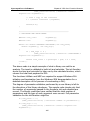
Figure 4-5. Combine Expert Opinions Dialog with First Expert's Data
Entered
Note that DPL has calculated the experience index to be about 145 for this
expert; this is analogous to saying the expert has about 145 observations
from which to draw conclusions, which seems reasonable given the
context. DPL has also calculated a weighted likelihood of 0.333 for this
expert.
DPL prompts you to enter the second (rank 2) expert.

For the rank 2 expert, enter the name In-house Expert. Enter the
following fractiles: 0.2, 0.28, 0.4.

Enter 0.2 for the overlap. You believe that your in-house expert (a
former government regulator) has about 20% overlap, i.e., 80% "new"
information compared with the government consultant.


Click the Add button. DPL updates the calculations.

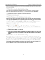
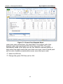
Click the Add button. The final results are shown in Figure 4-6.
Before examining results, add the third expert, named Third Opinion.
The fractiles are: 0.15, 0.25, and 0.5 and the overlap is 0.5.
64
Chapter 4: Multiple Experts
Syncopation Software
Figure 4-6. Final Combined Expert Opinions
DPL has calculated that the In-house expert has an experience factor of
about 39. The Third Opinion expert has an experience factor of only about
11.
The weights applied to the three experts are calculated and shown in the
far right column. The government consultant's assessment gets nearly 80%
of the weight, while the other two experts get about 17% and 3%,
respectively. The overall combined probability (likelihood) is 0.324. You
decide to use this probability in your analysis, and to also conduct
sensitivity analysis to see how decision sensitive it is.

Click OK to accept the probability as it is.
As shown in Figure 4-7, DPL has applied the combined probability to this
chance node, and noted that it comes from the Multiple Experts feature.
You can proceed to use this node in your model as you would use any
other two-state chance node.
65
Chapter 4: Multiple Experts
Syncopation Software
Figure 4-7. Node Data with Multiple Experts Data Defined
Note: As shown in Figure 4-7, when multiple experts data is in place, you
can no longer enter probabilities directly. In order to remove the multiple
experts data from the node, you would need to go back into the Multiple
Experts dialog and delete each expert. To do this, you select each expert
by clicking on his/her number in the far left column and then click Delete.
When there are no experts remaining in the dialog, click OK and the node
will be cleared of the multiple expert’s data.
66
Chapter 5: DPL Developer API
Syncopation Software
5 DPL Developer API
5.1 Overview
DPL Enterprise includes an Application Programming Interface (API), which
is an interface for controlling DPL from other programs. DPL's API can be
used to automate repetitive tasks, such as updating and running several
models. It can also be used to leverage DPL's decision analysis engine in
programs meant for use by persons not familiar with DPL or even decision
analysis.
Although using the DPL API requires some programming ability, common
tasks can be accomplished with only a few commands and do not require
specialist software development expertise. If you have written Excel
macros in Visual Basic for Applications (VBA), then you should have no
trouble learning to use the DPL API.
Most uses of the API involve creating one or more template Workspace
files as part of the development process. At runtime, the client application
controlling DPL supplies specific data and runs analyses to produce results.
These results can then be displayed to the user either by DPL or by the
client application.
The DPL API uses Automation (also called OLE Automation) as the
underlying technology for exposing capabilities to client programs.
Automation makes it easy to control DPL from current versions of Microsoft
Office. Future versions of the DPL API may employ other technologies.
The DPL API can be used with any language that supports Automation,
including the .NET family of languages. Code examples in this chapter are
written in VBA.
5.2 Controlling DPL from Visual
Basic
In this section, you will create a Visual Basic program that opens a DPL
Workspace file and runs a Decision Analysis. In what follows, we assume
67
Chapter 5: DPL Developer API
Syncopation Software
the client is Visual Basic for Applications (VBA) in Microsoft Excel 2010, but
the process is similar in any VB or VBA client environment.
5.2.1
Running a Decision Analysis
Before you can use DPL objects in a program, you need to register DPL as
a server. You do this by running DPL with the /Register switch.


Select Start | Run from Windows.

Add " /Register" (without quotes) after the path name and click OK.
Browse for DPL8.exe (normally in C:\Program Files
(x86)\Syncopation\DPL8).
DPL's splash screen will be visible for a second or so as DPL registers itself
with the system. You are now ready to begin using the DPL API.
You will start with a blank Excel workbook.




Start Microsoft Excel.
Click Developer | Code | Visual Basic.
Select Insert | Module.
Type the code below into the editor window.
Sub RunWildcat()
Dim oDPLApp As Object, oDPLWS
As Object
Set oDPLApp =
CreateObject("DPL.Application")
oDPLApp.Show =
1
Call oDPLApp.OpenWorkspace("C:\Wildcat.da")
Set oDPLWS = oDPLApp.Workspace
oDPLWS.RunDecisionAnalysisEnd Sub
You will need to change "C:\Wildcat.da" to the actual location of that
example file on your computer ("C:\Program Files
(x86)\Syncopation\DPL8\Examples\Wildcat.da" if you used the default
installation location when installing DPL).




Start DPL.
Return to the Visual Basic Editor.
Make sure the cursor is in the Sub RunWildCat.
Press F5 to run your Sub.
68
Chapter 5: DPL Developer API
Syncopation Software
Figure 5-1. Wildcat Policy Tree™
Note: if you run your macro before starting DPL, the CreateObject function
will create an invisible instance of DPL. You can make such an instance
visible using the Show property of DPLApplication (in the example above,
the line "oDPLApp.Show = 1" was included just in case).
In the above, you ran a Decision Analysis without specifying any options.
In the DPL API, run options are properties of the DPLWorkspace object
(oDPLWS).

Insert the two lines below before the RunDecisionAnalysis line.
oDPLWS.PolicyTree = 0
oDPLWS.InitialDecisionAlternatives = 1

Press F5 to run the Sub again.
69
Chapter 5: DPL Developer API
Syncopation Software
Figure 5-2. Wildcat Risk Profile
Lastly, you'll use the API to make a "what-if" change to the model to look
at a non-optimal alternative of the Test decision. To do that you'll use
branch control on the Test decision in the decision tree.


Add these lines to your Sub, replacing the two you previously added.
oDPLWS.PolicyTree = 1
Dim oDPLModel as
Object
Set oDPLModel = oDPLWS.MainModel
Dim
oDPLNode as Object
Set oDPLNode =
oDPLModel.Nodes("Test")
Dim oDPLTreeNode as
Object
Set oDPLTreeNode = oDPLNode.TreeNodes(1)
oDPLTreeNode.BranchControl = 0
oDPLModel.ClearMemory
Press F5 to run the Sub again.
70
Chapter 5: DPL Developer API
Syncopation Software
Figure 5-3. Wildcat Policy Tree™ with Test Controlled
5.2.2
Adding a Type Library Reference
If you would like DPL's object types (DPLApplication, DPLWorkspace, etc.)
to be known to your development environment, you can add a reference to
the DPL API type library. Doing so has the benefit that your development
environment can check syntax and provide lists of properties/methods.
Adding a reference is not required, and the examples in this chapter do not
assume that it has been done (in particular, they declare variables as type
Object rather than as a specific DPL object type).
The type information is contained in the main DPL executable (DPL8.exe).
To add a reference from Excel VBA, go to the Visual Basic Editor and follow
these instructions:



Select Tools | References....
Click Browse...
Change Files of Type to be Executable Files.
71
Chapter 5: DPL Developer API
Syncopation Software

Find your DPL executable. (C:\Program Files
(x86)\Syncopation\DPL8\DPL8.exe if you installed in the default
location).


Click Open.


Check the checkbox next to it if it isn’t already.
Scroll down in the Available Reference list to find "DPL 1.0 Type
Library"
Click OK.
Figure 5-4. Type Libary References
With the type library reference, you can use DPL types in your code, as in
the following example. Note that you still need to Dim the application as
Object (not as DPLApplication).
Sub RunWildcatTypes()
Dim DPLApp As Object
Set DPLApp = CreateObject("DPL.Application")
DPLApp.OpenWorkspace ("C:\Wildcat.da")
Dim WS
As DPLWorkspace
Set WS = DPLApp.Workspace
Dim Model As DPLModel
Set Model = WS.MainModel
Dim Node As DPLNode
Set Node =
72
Chapter 5: DPL Developer API
Syncopation Software
Model.Nodes("Test")
Dim TreeNode As DPLTreeNode
Set TreeNode = Node.TreeNodes(1)
TreeNode.BranchControl = 0
Model.ClearMemory
WS.RunDecisionAnalysisEnd Sub
Test the Type Library now.


Enter the new Sub into Module1.


Press F5 to run it.
Change the path from "C:\Wildcat.da" to where the file is on your
computer.
Note: if you place your cursor next to the WS on the last line of the
Sub and type ".", Excel provides you with a list of Methods and
Properties of a DPLWorkspace.
5.3 API Objects and Types
DPL's API provides several objects which allow you to manipulate the
application, its documents and their data. The figure below shows the
hierarchical relationships of the DPL API objects.
DPLApplication (1 per running instance of DPL)
→DPLWorkspace (1)
→DPLModel (0 or
more)
→DPLNode (0 or more)
→DPLTreeNode (0 or more)
→DPLResult (0 or more)
Figure 5-5. DPL API Objects
5.3.1
The DPLApplication Object
The Application object represents a running instance of DPL. It is the
starting point for any conversation with the DPL API.
The methods of the Application object correspond to activities that effect
the whole application and not just individual windows (e.g., Models, Risk
Profile Charts, etc). Most methods in the Application object correspond to
commands in the File menu.
The code below obtains a reference to a DPLApplication object.
Dim oDPLApp As ObjectSet oDPLApp =
CreateObject("DPL.Application")
73
Chapter 5: DPL Developer API
5.3.2
Syncopation Software
The DPLWorkspace Object
The DPLWorkspace object corresponds to a DPL Workspace (.DA) file. Only
one Workspace file can be loaded at a time. DPL creates a blank
Workspace when it starts. The currently loaded Workspace can be
accessed using the Workspace property of the DPLApplication object.
Dim oDPLWS As ObjectSet oDPLWS = oDPLApp.Workspace
5.3.3
DPLModel Objects
DPLModel objects correspond to components of a DPL Workspace that can
be run or evaluated, including Models, Programs and Commands.
Dim oDPLModel as Object, oDPLModel2 as ObjectSet
oDPLModel = oDPLWS.MainModelSet oDPLModel2 =
oDPLWS.Models("Another Model")
A DPLModel object can be any of the types shown in Table 5-1 below (see
the Type property).
ID
Hex value
(decimal value)
Description
ID_DOC_TYPE_IDDT
0x0001 (1)
Model (influence diagram and
decision tree)
ID_DOC_TYPE_PROGRAM
0x0002 (2)
Program not run directly
ID_DOC_TYPE_DRIVER_PROGRAM
0x0004 (4)
Runnable program
ID_DOC_TYPE_COMMAND
0x0005 (5)
Command
Table 5-1. DPLModel Types
5.3.4
DPLNode Objects
DPLNode objects correspond to nodes in a DPL influence diagram. A
DPLNode object is returned by the Nodes property (collection) of a
DPLModel object.
Dim oDPLNode1 as ObjectSet oDPLNode1 =
oDPLModel.Nodes("Revenue")
5.3.5
DPLTreeNode Objects
DPLTreeNode objects correspond to nodes in a DPL decision tree. Each
decision tree node is an instance of an influence diagram node of type
74
Chapter 5: DPL Developer API
Syncopation Software
Decision, Chance or Controlled. A DPLTreeNode object is returned by the
TreeNodes property (collection) of a DPLNode object.
Dim oDPLTreeNode1 as ObjectSet oDPLTreeNode1 =
oDPLNode1.TreeNodes(1)
5.3.6
DPLResult Objects
DPLResult objects correspond to components of a DPL Workspace that are
the result of analyses, such as Policy Trees™, Risk Profile Charts, Rainbow
Diagrams, etc.
Dim oDPLResult as ObjectSet oDPLResult =
oDPLWS.Results("Expected Value")
A DPLResult object can be any of the types shown in Table 5-2 below (see
the Type property).
ID
Hex value
(decimal value)
Description
ID_DOC_TYPE_ENDPOINTS
0x0010 (16)
Endpoints
ID_DOC_TYPE_RISK_PROFILE
0x0020 (32)
Risk Profile chart
ID_DOC_TYPE_DECPOLICY
0x0021 (33)
Policy Tree™
ID_DOC_TYPE_POLICYSUM
0x0022 (34)
Policy Summary™
ID_DOC_TYPE_SENS
0x0023 (35)
Rainbow diagram (one-way)
ID_DOC_TYPE_TWOWAY_SENS
0x0024 (36)
Rainbow diagram (two-way)
ID_DOC_TYPE_VAL_COMP
0x0025 (37)
Value tornado diagram
ID_DOC_TYPE_NOM_COMP
0x0026 (38)
Base case tornado diagram
ID_DOC_TYPE_EVENT_COMP
0x0027 (39)
Event tornado diagram
ID_DOC_TYPE_VOIC
0x0028 (40)
Value of info/control chart
ID_DOC_TYPE_CORR
0x0029 (41)
Value correlations chart
ID_DOC_TYPE_OPTION_VALUE
0x002A (42)
Option value chart
Table 5-2. DPLResult Types
75
Chapter 5: DPL Developer API
5.3.7
Syncopation Software
Parameter Data Types
The DPL API uses the five data types described below. Examples of how to
declare them in VB and C/C++ are given after each description. Note that
in VB one can also use Variants for any type. The Variant subtypes (VT_*)
are shown in the comments.
Object: An OLE Automation IDispatch pointer. Dim o as Object
'VB VT_DISPATCH
LPDISPATCH lpDispatch; // C/C++
Double: A double precision floating point number, which can take values in
the range of 2.2250738585072014e-308 to 1.7976931348623158e+308.
Dim d as Double
'VB VT_R8
double d;
//
C/C++
Long: A 32-bit signed integer, which can take values in the range of
­2147483648 to 2147483647. Dim i as Long
'VB VT_I4
int i;
// C/C++
Bool: A Long value interpreted to be boolean (zero for false, nonzero for
true). Dim b as Long
'VB VT_I4
BOOL b;
//
C/C++
String: An OLE Automation BSTR string.
'VB VT_BSTR _bstr_t s;
Dim s as String
// C/C++
5.4 API Reference
This section documents the properties and methods of each type of object
in the DPL API.
The syntax for properties is:
property_name : type[DPL Type Library type].
The property declaration is followed by a parenthetic comment indicating
whether the property is read-only or read/write.
The syntax for methods is:
method_name(param1 : param1 type, param2 : param2 type, …)
76
Chapter 5: DPL Developer API
Syncopation Software
5.4.1
DPLApplication Properties
DisplayRunStatus : Bool (read/write)
Controls whether or not DPL displays the run status dialog when running
an analysis. The default is false if DPL was started by Automation, true
otherwise.
ErrorsToLog : Long (read/write)
Controls the display of error and warning messages that would normally be
displayed in message boxes. Must be one of the following:
0
Display interactively with message boxes
Print in session log
2
Both
1
LastError : String (read-only)
A string describing the last error (or warning) from DPL, whether or not
that error was displayed. In most cases, the string in LastError will be the
same as the description property of the VB Err object.
On Error GoTo OnErr
... 'code that
results in an errorOnErr:
MsgBox
Err.Description
MsgBox oDPLApp.LastError 'same
as above
LogFile : String (read/write)
The path of a text file for the session log. Log messages will be printed
both to the Session Log window and the specified file.
The file will be opened immediately and will stay open until the DPL
Application instance is released. Any existing file of the same name will be
overwritten. To close the file explicitly, set LogFile to "" (an empty string).
Options(Name : String) : Long (read/write)
Reserved for future use. There are no DPLApplication named options at this
time.
PostRunExcelMacro : String (read/write)
Contains the name of an Excel macro that DPL should run at the end of an
analysis. Using this property with the RunAsynchronous property, you can
77
Chapter 5: DPL Developer API
Syncopation Software
have your client program start a DPL analysis and return to an idle state,
then you can have DPL pass control back to the client after the analysis.
With this technique, you can run a DPL analysis from a VBA macro in an
Excel workbook which is itself linked to DPL and will be used in the
analysis. See the DrugDevelopmentRunButton example files.
ReleaseNumber : Long (read-only)
The DPL release number as an integer. For example, DPL release 8.01.02
would return the integer 80102.
RunAsynchronous : Bool (read/write)
When this property is true, calls to DPL "Run" methods will return
immediately. When false (the default), they will return when the analysis is
complete. You can use this method to "kick off" a run in a situation where
the results will be examined interactively by the user, or you can use it in
conjunction with the PostRunExcelMacro to take back control after the
analysis (if the client is Excel).
Show : Long (read/write)
The current state of the DPL main window. Set this property to maximize,
minimize, show or hide DPL's main window. The appropriate values are
those of the Windows API ShowWindow command, a few of which are
listed below. Consult the Windows API documentation for details.
SW_HIDE
0
SW_SHOWMINIMIZED 2
SW_SHOWNORMAL
1
SW_SHOWMAXIMIZED 3
If DPL is started by Automation (e.g., by using
CreateObject("DPL.Application") in VBA) when no instance of DPL is
running, DPL's main window will initially be hidden.
Workspace : Object[DPLWorkspace] (read-only)
This method returns a DPLWorkspace object corresponding to the currently
loaded DPL Workspace file. If no Workspace is loaded, DPL will throw an
exception.
78
Chapter 5: DPL Developer API
Syncopation Software
5.4.2
DPLApplication Methods
CloseWorkspace()
Closes the current Workspace file without prompting.
Exit(Code : Long)
Terminates the DPL Application returning Code to the system (e.g., use
Exit(0) for "normal" termination). Note that the call is asynchronous, so
DPL may still be running when the method returns.
NewWorkspace()
Creates a new, blank Workspace file. If a Workspace was previously
loaded, it is closed.
OpenWorkspace(Path : String)
Opens the Workspace file indicated by Path.
SaveWorkspace()
Saves the Workspace file using the current file name and path. The
Workspace file must be named otherwise DPL will throw an exception.
SaveWorkspaceAs(Path : String)
Saves the Workspace file to Path.
Warning(message : String)
Causes DPL to display a message box containing message.
WriteToLog(message : String), WriteLnToLog(message : String)
Writes message to the session log. WriteLnToLog appends a new line, so
that the next log message will start in the first column of the following line.
To send a multi-line message to the session log, include carriage return /
linefeed pairs ("\r\n" in C/C++, Chr$(13)+Chr$(10) in VB).
79
Chapter 5: DPL Developer API
5.4.3
Syncopation Software
DPLWorkspace Properties
Distribution : Long (read/write)
The type of risk profile(s) DPL should generate in the next run. Must be
one of the following:
0
No distribution 1
Objective function
2
Objective function and all attributes
3
All attributes
One attribute
4
If the value is 4, DistributionIndex should be set to the index of the desired
attribute.
DistributionGraphFormat : Long (read/write)
Controls how the risk profile generated in a Monte Carlo simulation run is
displayed.
0
Cumulative
1
Histogram
This has no effect on risk profiles generated in Decision Analysis runs,
which are always displayed in Cumulative form.
DistributionIndex : Long (read/write)
The index of the attribute for which a risk profile should be generated in
the next run. Ignored unless Distribution is set to 4.
DistributionIntervals : Long (read/write)
The number of distribution intervals DPL should use for the risk profiles
generated in the next run. Must be between 0 and 10000. Default is 500.
For Monte Carlo simulation runs, this property can be set to -1, indicating
that DPL should store all samples and do no aggregation.
EvaluationMethod : Long (read/write)
The evaluation method DPL should use in the next run. Must be one of the
following:
0
2
Fast sequence evaluation
Discrete Tree Simulation
80
1
Full enumeration
Chapter 5: DPL Developer API
Syncopation Software
FatPolicy : Bool (read/write)
True if DPL should produce Fat Policy™ (i.e., rolled-back expected values
for all attributes) in the next run. Ignored if there is only one attribute.
InitialDecisionAlternatives : Bool (read/write)
True if DPL should generate a risk profile chart showing initial decision
alternatives in the next run. Ignored if the tree doesn't start with a decision
or if it starts with a decision having more than eight alternatives.
MainModel : Object[DPLModel] (read-only)
An object reference to the main model of the currently loaded Workspace
file. Returns Null if no Workspace is loaded or the current Workspace has
no main model.
Dim oDPLModel As ObjectSet oDPLModel =
oDPLApp.MainModel
Note that this property is read-only. To change the main model, use the
Models property to obtain an object reference to the model you want to
make main, then call its MakeMain property.
Models(Name : String) : Object[DPLModel] (read-only)
An object reference to the model with title Name. Returns Null if there is no
model (DPL Model or Program window) with title Name in the Workspace.
The example below displays the type of a model named "Bob".
Dim oDPLModel As ObjectSet oDPLModel =
oDPLApp.Model("Bob")If oDPLModel Is Nothing Then
MsgBox "Sorry, no Bob in the Workspace"Else
MsgBox "Bob is type " +
Str(oDPLModel.Type)End If
Options(Name : String) : Long (read/write)
Used to set various options not having their own properties. Currently the
following options are recognized:
DecimalPlaces OutputScaling
(Bool) DecimalPlacesProbs
ZeroEquivalent ProbsAsPercents
These control display as per the similarly named options in File | Options |
Outputs.
81
Chapter 5: DPL Developer API
Syncopation Software
PolicyLevels : Long (read/write)
The number of policy levels DPL should include in the Policy Tree™ in the
next run. Default is all levels. A value of 1 is treated as 2, since the Policy
Tree™ requires two or more levels.
PolicySummary : Bool (read/write)
True if DPL should generate a Policy Summary™ in the next run.
PolicyTree : Bool (read/write)
True if DPL should generate a Policy Tree™ in the next run.
RecordEndpoints : Bool (read/write)
True if DPL should record endpoints in the next run. Requires that the
evaluation method be full enumeration otherwise it is ignored.
Results(Name : String) : Object[DPLResult] (read-only)
An object reference to the result with title Name. Returns Null if no
Workspace is loaded or there is no result with the title Name in the
Workspace. See the Model property for an example.
SamplesInitial : Long (read/write)
The initial number of samples for a Monte Carlo simulation run or a
Decision Analysis run using discrete tree simulation evaluation method.
SamplesRestart : Long (read/write)
The minimum number of samples following each decision in a Monte Carlo
simulation run or a Decision Analysis run using discrete tree simulation
evaluation method. Has no effect if the model does not contain decisions.
TimeSeriesFromAtt : Long (read/write)
The index of the first attribute to be displayed in the next Time Series
Percentiles run. Note that the first attribute has index 1 (not 0).
82
Chapter 5: DPL Developer API
Syncopation Software
TimeSeriesInitialPeriod : Long (read/write)
The number displayed for the first attribute on the x-axis in the Time Series
Percentiles graph. For example, if each attribute represents cash flow in a
given year, and the first attribute corresponds to 2010, you would set this
property to 2010.
TimeSeriesNumPeriods : Long (read/write)
The number of time periods (attributes) to be displayed in the next Time
Series Percentiles run. For example, if there are five attributes
corresponding to years 2014-2018, you would use:
oDPLWS.TimeSeriesFromAtt =
1oDPLWS.TimeSeriesNumPeriods =
5oDPLWS.TimeSeriesInitialPeriod =
2014oDPLWS.RunTimeSeries
Title : String (read-only)
The file name of the Workspace (e.g., "Wildcat.da"). This property is readonly; use the DPLApplication method SaveWorkspaceAs() to rename the
Workspace.
ValueCorrelations : Long (read/write)
True if DPL should generate a Value Correlations chart in the next Decision
Analysis or Monte Carlo run. For a Decision Analysis, Value Correlations
require that the evaluation method be full enumeration.
ValueOfInfoControl : Bool (read/write)
True if DPL should generate an Expected Value of Perfect
Information/Control chart in the next Decision Analysis run. Ignored if the
number of PolicyLevels is not the maximum for the decision tree.
5.4.4
DPLWorkspace Methods
CreateProgram(Data : String, Name : String, Driver : Bool)
Creates a DPL Program in the current Workspace with the DPL code
contained in Data and the title Name. Driver should be True if the program
can be run directly, or False if the program is intended as an include file to
83
Chapter 5: DPL Developer API
Syncopation Software
be referenced by another program or a Model. The example below creates
and runs a simple program.
Dim Data As StringData = "chance c.{lo,hi} = {0.5}
= 1,2;" _
& "sequence: " _
& "gamble on c
and get c"oDPLApp.CreateProgram(Data, "C", 1)Dim
oDPLModel as ObjectSet oDPLModel =
oDPLApp.Model("C")oDPLModel.MakeMainoDPLWS.RunDeci
sionAnalysis
This method is convenient for small programs, such as those supplying
data used to initialize nodes in a template influence diagram. However for
large programs, writing a .dpl file to disk and calling ImportProgram is
more efficient.
ImportProgram(Path : String, Name : String, Driver : Bool)
Imports the program (.dpl source file) specified by Path into the current
Workspace and gives it the title Name. Driver should be true if the program
can be run directly, or false if the program is intended as an include file to
be referenced by another Program or a Model.
RunDecisionAnalysis()
Runs a Decision Analysis. To specify run options, use the following
properties: EvaluationMethod, Distribution, DistributionIndex,
InitialDecisionAlternatives, ValueCorrelations, PolicyTree, PolicyLevels,
FatPolicy, PolicySummary, ValueOfInfoControl. These properties have the
same meanings and defaults as in the Home | Run group.
The example below runs a Decision Analysis generating a Risk Profile but
no Policy Tree™.
oDPLWS.Distribution = 1oDPLWS.PolicyTree =
0oDPLWS.RunDecisionAnalysis
RunMonteCarloSimulation()
Runs a Monte Carlo simulation. To specify run options, use the following
properties: SamplesInitial, SamplesRestart, Distribution,
InitialDecisionAlternatives, DistributionIntervals, DistributionGraphFormat,
ValueCorrelations, PolicySummary, PolicyLevels, PolicyTree. These
properties have the same meanings and defaults as in the Home | Run
group.
84
Chapter 5: DPL Developer API
Syncopation Software
RunOptionValue()
Runs an Option Value analysis. DPL will use the default decision
alternatives as specified in Node Definition General. Or you may specify
defaults by using the DPLNode DefaultState property before the run.
RunTimeSeries()
Runs a Time Series analysis. See the TimeSeriesNumPeriods property for
an example.
RunTornado(type : Long, option : Long)
Runs a tornado diagram. The type of tornado is determined by the type
and option parameters. The valid combinations are shown below in Table
5-3.
type
opt
Tornado Type
37
0
Value
38
0
Base Case
38
1
Initial Decision Alternatives
39
0
Event (Deterministic)
39
1
Event (Probabilistic)
Table 5-3. Tornado Types
Note that 37, 38 and 39 correspond to the DPLResult Type values of the
charts produced by the run. The example below runs a Base Case Tornado.
oDPLWS.RunTornado(38, 0)
UpdateAllResults()
This method refreshes all output (DPLResult) windows. This may be
necessary after changing options that effect display.
oDPLWS.Options("DecimalPlaces") =
1oDPLWS.UpdateAllResults
85
Chapter 5: DPL Developer API
5.4.5
Syncopation Software
DPLModel Properties
EvalResultEV : Double (read-only)
The expected value (EV) results of the most recent Decision Analysis run.
EvalResultCE : Double (read-only)
The certain equivalent (CE) results of the most recent Decision Analysis
run.
EvalResultsValid : Long (read-only)
Indicates whether evaluation results (e.g., EvalResultEV) exist. The value
will be 0-2 with the following meanings.
0
Results not valid
1
Results valid from a
Decision Analysis run 2
Results valid from a Monte Carlo simulation
run
IncludeEnd : String (read/write)
See IncludeStart.
IncludeStart : String (read/write)
Used to set the name of the includes (DPL Programs) referenced by the
Model. IncludeStart corresponds to the "DPL Program for Data Definitions"
in the Model Links dialog; IncludeEnd corresponds to "DPL Calculation
Program".
Nodes(Name : String) : Object[DPLNode] (read-only)
Used to obtain an object reference to a node (DPLNode) in the model with
title or variable name Name. See the DPLNode property VariableName for
an explanation of node titles and variable names. Returns Null if no such
node exists in the DPLModel.
Dim oModel As Object
Set oModel = WS.MainModel
oModel.Nodes("Test")
86
Dim oNode As Object
Set oNode =
Chapter 5: DPL Developer API
Syncopation Software
Options(Name : String) : Long (read/write)
Reserved for future use. There are no DPLModel named options at this
time.
Title : String (read/write)
The title of this DPLModel object, as displayed in the Workspace Manager.
Type : Long (read-only)
The type of this DPLModel object. See Table 1 for a list of DPLModel types.
5.4.6
DPLModel Methods
Delete()
Deletes the associated document from the Workspace.
MakeMain()
Makes this document the main model, that is, the document that will be
run in the next analysis. This DPLModel must be of type Model (influence
diagram / decision tree) or a driver program. If the model is not of one of
these types, DPL throws an exception.
ClearMemory()
Deletes compile structures and removes any volatile (unrenamed) outputs
associated with this model. Same as Home | Run | Clear Mem.
If you run an analysis and then modify the model, you will need to issue a
ClearMemory command to force the model to be recompiled.
5.4.7
DPLNode Properties
DefaultState : Long (read/write)
The default state of this node as set in the General tab of the Node
Definition dialog and as used by Base Case tornadoes and Option Value
charts. The first state has index 0. The value -1 indicates there is no
default.
87
Chapter 5: DPL Developer API
Syncopation Software
Dim oDPLNode as ObjectSet oDPLNode =
oDPLModel.Nodes("Drill")oDPLNode.DefaultState = 1
'No
Name : String (read/write)
The title or name of the node. Note that this string will include carriage
return/linefeed pairs if the node name is on more than one line. If there
are instances of this node in the decision tree, their names will be changed
as well. A node name can contain characters not valid in a DPL variable
name, such as punctuation and whitespace. Use the VariableName
property to get the name as sanitized for use in expressions.
Probabilities(Index : Long) : String (read/write)
The probabilities of the node. The individual probabilities are indexed as
they appear in the Data tab (or Probabilities tab if separately conditioned)
of the Node Definition dialog, with the topmost branch being index 0. The
probabilities are stored as strings even if they are constant numbers.
SensHigh : Double (read/write)
See SensLow.
SensLow : Double (read/write)
SensLow and SensHigh are the Low and High values used for each bar in
Value tornado diagrams. They can only be set for unconditioned, constant
value nodes.
Dim oDPLNode1 as Object, oDPLNode2 as ObjectSet
oDPLNode1 = oDPLModel.Nodes("Sales")Set oDPLNode2
= oDPLModel.Nodes("Costs")oDPLNode1.SensLow =
1.3oDPLNode1.SensHigh = 1.9oDPLNode2.SensLow =
0.7oDPLNode2.SensHigh = 1.1oDPLWS.RunTornado(37,
0)
TreeNodes(Index : Long) : Object[DPLTreeNode]
Used to obtain an object reference to a decision tree node (DPLTreeNode)
in the model which is an instance of this influence diagram node
(DPLNode). If there is only one instance of this node in the decision tree, it
will have index 1. If there are several instances, the instance number is
88
Chapter 5: DPL Developer API
Syncopation Software
shown in the title bar of the Node Definition dialog when you double-click
on a node in the decision tree.
Type : Long (read-only)
The type of this node. The type is one of the following:
0
Value
Decision
1
Chance 2
Controlled
3
Values(Index : Long) : String (read/write)
The values of the node. The individual values are indexed as they appear in
the Data tab (or Values tab if separately conditioned) of the Node
Definition dialog, with the topmost branch being index 0. The values are
stored as strings even if they are constant numbers.
Dim oDPLNode1 as ObjectSet oDPLNode1 =
oDPLModel.Nodes("Costs")'Costs is a three-state
chance nodeoDPLNode1.Values(0) =
"10"oDPLNode1.Values(1) = "12"oDPLNode1.Values(2)
= "15"
VariableName : String (read-only)
The variable name of the node for use in expressions. If the node name is
a valid identifier (that is, it begins with a letter and consists of letters,
numbers and underscores) then the variable name is simply the node
name. If not, the variable name is the node name with invalid characters
replaced with underscores ('_'). For example, if the node name is "R&D
Costs", the variable name is "R_D_Costs".
5.4.8
DPLTreeNode Properties
BranchBlock : String (read/write)
Used to block (temporarily remove from consideration) certain branches of
a decision node. The format of the string is a comma separated list of ones
and zeroes, one for each decision alternative. A zero indicates that that
alternative is blocked.
Dim oDPLNode1 as ObjectDim oDPLTreeNode1 as
ObjectSet oDPLNode1 = oDPLModel.Nodes("Invest")Set
oDPLTreeNode1 = oDPLNode1.TreeNodes(1)'Block the
89
Chapter 5: DPL Developer API
Syncopation Software
second of three
alternativesoDPLTreeNode1.BranchBlock = "1,0,1"
Set BranchBlock to an empty string ("") to unblock all branches.
Note that changing the BranchBlock state of a tree node will overwrite the
BranchControl state and vice versa. If you use this method on a TreeNode
that is not a decision node, DPL throws an exception.
BranchControl : Long (read/write)
Used to temporarily control a decision or chance node to a given state.
Zero corresponds to the first state. The value -1 indicates that the tree
node is not controlled.
'Control the node to its first
stateoDPLTreeNode1.BranchControl = 0
Note that changing the BranchControl state of a tree node will overwrite
the BranchBlock state and vice versa.
Name : String (read/write)
The name of the tree node. Note that this string will include carriage
return/linefeed pairs if the name is on more than one line. Changing the
name of a tree node does not change the name of the influence diagram
node of which it is an instance.
Type : Long (read-only)
The type of this tree node. The types are the same as those of influence
diagram nodes (see Type in DPLNode). Only decision and chance nodes
appear in the decision tree.
5.4.9
DPLResult Properties
Options(Name : String) : Long (read/write)
Reserved for future use. There are no DPLResult named options at this
time.
Title : String (read/write)
The title of this DPLResult object, excluding the type prefix. For example, a
Risk Profile Chart might have the title "Expected Value".
90
Chapter 5: DPL Developer API
Syncopation Software
Type : Long (read-only)
The type of this DPLResult object. See Table 5-2 for a list of DPLResult
types.
5.4.10
DPLResult Methods
CopyPicture(Long : format)
Copies a picture of the associated window to the Windows clipboard. If
format is 0, the picture is a bitmap; if it is 1, the picture is a metafile.
Delete()
Deletes the associated document from the Workspace.
Export(Path : String)
Exports the associated document to the comma separated value (CSV) or
XML file in Path. The format is determined by the file extension of Path,
which must be either ".CSV" or ".XML".
ReduceDist(Index : Long, Name : String, NumStates : Long, Format : Long)
Reduces a distribution to a chance node. This method is only valid for Risk
Profile charts. Index indicates which of the risk profile datasets displayed in
the chart should be reduced, the first one being index 0.
The node will be called Name and will have NumStates outcomes. The
output is determined by the Format parameter:
1
Both
DPL session log 2
Windows clipboard
91
3
Chapter 5: DPL Developer API
Syncopation Software
92
Chapter 6: DPL User Function Libraries
Syncopation Software
6 DPL User Function
Libraries
6.1 Overview
One way to extend the functionality of DPL is to create a Windows DLL
with functions to be called from your DPL models. A DPL DLL can also
serve as a way to interface DPL with other programs, such as software
packages performing detailed economic calculations for specific industry
verticals. Calling a function in a DPL DLL involves very little overhead, so a
DLL can be attractive in situations where runtime performance is critical.
Implementing a DPL DLL requires technical expertise and significant effort,
so before starting such a project you should consider whether more highlevel mechanisms such as running Excel macros, database initialization
links or the DPL Developer API would better meet your needs.
6.2 Technical Considerations
A DPL user function library must have a file extension of .DLL. Each library
may contain one or more user functions in addition to the standard
functions required by the Windows DLL mechanism. There is no limit to the
number of libraries that may be in use during a DPL session. A library is
loaded the first time it is encountered during the compilation of a DPL
model, program or command procedure. A library is released by Windows
only when all DPL sessions that have referenced the library are terminated.
At the time a library is loaded, it must reside in the current directory or in a
directory included in the PATH environment variable.
Though a library can behave as a full Windows application, it is
recommended that a library constrain itself to providing computational
functions suitable for execution during a DPL analysis.
User functions are divided into two categories: functions called implicitly by
DPL, and functions called explicitly by DPL programs and command
procedures. Implicitly called functions are optional. When a library is
loaded, DPL checks for the presence of certain predefined function entry
points. At various times during a DPL session, these entry points are called,
such as when an analysis is starting or ending. Explicitly called functions
93
Chapter 6: DPL User Function Libraries
Syncopation Software
are referenced by expressions in DPL models, which are then executed
when the expressions are evaluated.
User functions may be written in any language that complies with the
requirements of a native Windows DLL. The examples used in this
specification (including the sample code) have been prepared for use with
the Microsoft Visual Studio C++ compiler.
All functions receive at least one parameter, which is the number of
additional parameters passed to the function. This will allow for future
expansion of the parameter list for each function. A function can check that
the number of parameters received are correct and terminate via the error
call-back function if it is not (parameter mismatches will generally result in
a crash). Alternatively, a library may check the DPL version number
supplied with the load function to ascertain whether the number of
parameters for subsequent calls will be correct.
User functions may call certain DPL functions as part of their execution.
When a library is loaded, it is passed a list of function entry points in DPL.
These functions provide access to DPL features, such as writing to the DPL
Log or accumulating distribution data.
All definitions required to interface with DPL are provided in an include file
called dpluserf.h. This file should be included in the DLL source after
windows.h and any required C language include files. A Zip file containing
the sample code and these include files can be obtained from Syncopation
support.
6.3 Implicit Functions
6.3.1
Load Library
This function is called the first time a DPL session compiles a program or
command procedure that references a DLL. Note that each DPL session
that references a DLL will call the load function. If a DLL cannot operate
with more than one session at a time (e.g., because of its use of static
storage), it must reject the load attempt by calling the DPL error function.
This function is passed a list of entry points within DPL that may be used to
perform various services during subsequent library function calls. A
function definition macro for the load function is provided in the dpluserf.h
include file. Another include file, load.h, is also provided for validating and
saving the entry point list (see the sample code).
94
Chapter 6: DPL User Function Libraries
Syncopation Software
Typical functions performed by the load function include:
•
•
•
•
•
•
•
Saving the list of DPL function entry points
Writing a sign-on/copyright message to the DPL Log
Verifying that the library is not already active
Opening files that will be used during subsequent processing
Allocating global memory and other Windows objects
Creating a window to provide a custom interface to the user
Controlling sequence optimization during subsequent analyses
Name:
load
Parameters:
1. Integer number of parameters (= 3)
2. Pointer to an array of pointers to functions
3. Integer number of elements in the array of parameter 2
4. Integer DPL version number (e.g., 0x00080000 => Release 8.0)
Returns:
0 : Fast sequence evaluation is not allowed in this library
1 : Fast sequence evaluation is allowed
Fast sequence evaluation (the fastest exact evaluation method) should not
be allowed if the library requires that all decision tree paths be executed
during a decision analysis; e.g., if the library matches each call to data
obtained from a disk file. This function should not return if the load is to be
aborted (call the error function instead as defined below).
6.3.2
Unload Library
This function is called when a DPL session that previously called the
library's load function is terminated. The library is not released until all DPL
sessions that have referenced the library are terminated. Libraries that
need to perform termination processing before being released by Windows
should maintain a count of the active sessions connected to the library and
perform final processing when the count reaches zero.
Typical functions performed by the unload function include:
•
•
•
Closing open files
Deallocating global memory and other Windows objects
Destroying any windows created by the library
95
Chapter 6: DPL User Function Libraries
Syncopation Software
Name:
unload
Parameters:
1. Integer number of parameters (= 0)
Returns:
(None)
6.3.3
Begin Analysis
This function is called prior to beginning an analysis of a compiled DPL
program. Analyses result from executing any of the Run menu functions.
Performing a tornado diagram or rainbow diagram will result in multiple
analyses.
The function should prepare the library for subsequent function calls during
an analysis. Typical functions performed by the begin analysis function
include:
•
•
•
Initializing variables used during an analysis
Opening or repositioning files for endpoint input or output
Allocating temporary memory and other Windows objects
Name:
begin_analysis
Parameters:
1. Integer number of parameters (= 0)
Returns:
(None)
6.3.4
End Analysis
This function is called after an analysis has completed.
Typical functions performed by the end analysis function include:
•
•
Closing open files
Deallocating temporary memory and other Windows objects
96
Chapter 6: DPL User Function Libraries
Syncopation Software
Name:
end_analysis
Parameters:
1. Integer number of parameters (= 0)
Returns:
(None)
6.3.5
Reset (error recovery)
This function is called during DPL error processing. The cause of the error
may or may not relate directly to the library and may or may not have
occurred during an analysis. The library should perform whatever recovery
processing is required to guarantee that it is prepared to receive
subsequent function calls.
Typical functions performed by the reset function include:
•
•
Calling the end_analysis function, if appropriate
Deleting output files
Name:
reset
Parameters:
1. Integer number of parameters (= 0)
Returns:
(None)
6.3.6
Window Functions
This function is called whenever DPL needs to disable all DPL windows or
enable all DPL windows. This function must be implemented by libraries
that create their own windows.
Name:
window_functions
Parameters:
1. Integer number of parameters (= 2)
2. Integer indicating the required window function
3. Window handle
97
Chapter 6: DPL User Function Libraries
Syncopation Software
Returns:
An integer (BOOL) indicating whether the window handle parameter
matches a window owned by the library
Consider the follow code fragment:
#include "dpluserf.h"
BOOL CALLBACK WINDOW_FUNCTIONS( int function, HWND hWnd )
{
switch( function ) {
case WF_ENABLE:
if( hLibWnd )
EnableWindow( hLibWnd, TRUE );
break;
case WF_DISABLE:
if( hLibWnd )
EnableWindow( hLibWnd, FALSE );
break;
case WF_ROTATE:
return( hWnd == hLibWnd );
}
return( YES );
}
Here, it is assumed that the library has created a window and saved its
handle in the variable, hLibWnd. For the enable and disable functions, the
window is enabled or disabled if the window handle is valid. Note that the
window handle parameter is ignored and the function always returns 1,
defined as YES. For the rotate function, the window handle parameter is
compared with the library window handle and the result of the comparison
is returned.
6.4 Explicit Functions
Explicit functions are the functions you write and call from your DPL
models.
Explicit functions behave in much the same way as DPL built-in functions:
they are coded in DPL expressions, receive numbers and strings as
parameters, and return a double precision floating point number.
98
Chapter 6: DPL User Function Libraries
Syncopation Software
An explicit function is referenced in a DPL expression by coding the name
of the library, optionally followed by a period and the function entry point
name, then a parenthesized argument list. The library name may not
include a path specification. At the time the library is loaded, it must exist
either in the current directory or in a directory in the current path.
If a period and function entry point name do not follow the library name,
the default entry name, calculate, will be used. The argument list consists
of from 0 to 127 expressions or strings separated by commas. The
following are all valid explicit function references:
mylib()
mylib.calculate( 1, x+y )
mylib.filename( "c:\\dpl\\test.dat" )
All functions should begin with the following line:
extern "C" double CALLBACK name( int num_parms, double
argument[], int num_args )
where name is the name of the function. This provides the following
required definitions:
•
•
•
The routine observes the appropriate calling convention
The function returns a double precision floating point number
The function accepts three parameters:
1. The number of parameters (= 2)
2. A pointer to an array of double precision floating point
numbers
3. The integer number of elements in the array specified by
parameter #2.
Although an explicit function reference is coded in DPL with separate
arguments, the library function always receives three parameters. The
parameters passed by the explicit function are placed into the array
accessed by the second parameter above. For example:
mylib(1,2,3,4)
would result in three parameters being passed to the library:
1. The number of additional parameters (always 2)
2. A pointer to an array of four elements containing the numbers 1, 2,
3, and 4
3. The number 4 (the number of elements in the array)
An empty explicit function reference argument list, such as mylib()above,
would still result in three parameters; however, the second parameter
would be a null pointer and the third parameter would be zero.
99
Chapter 6: DPL User Function Libraries
Syncopation Software
String pointers are passed to the library as specially encoded floating point
numbers. An attempt to use one of these numbers in ordinary arithmetic
will result in a floating point math error. The include file dpluserf.h contains
two macros for dealing with these numbers:
IS_STRING_ARG( p )
This macro tests a double precision floating point number to
see if it is a string argument pointer. It evaluates to one
(TRUE) if the number is a string pointer and a zero (FALSE) if it
is not.
STRING_ARG( p )
This macro returns the string argument pointer encoded in the
double precision floating point number.
The follow code fragment illustrates the use of the string macros.
if (IS_STRING_ARG(argument[0])) {
int len = strlen(STRING_ARG(argument[0]));
} else
...
(*DPL_functions.error)( "Not a string!" );
The parameter count, the argument count, and the IS_STRING_ARG macro
may be used to perform parameter validation by a library function.
The values in the array parameter are passed by value. This means that
any changes made to them within the function will not affect values in the
DPL model (i.e., the array parameter entries may be used as local
variables). Strings pointed to by string argument pointers should not be
modified. Doing so may cause unpredictable results.
All explicit functions must return a valid double precision floating point
number. This number will be used to complete expression evaluation at the
point where the function reference occurred within the DPL model.
If all explicit function reference arguments are constants, a call will be
performed to the function only once at compile-time. Otherwise, a call will
be performed each time the containing expression is evaluated and one or
more arguments have changed in value unless the library's load function
indicated that no optimizations should be performed. In this case, a call will
be made each time the containing expression is evaluated whether or not
any arguments have changed in value.
100
Chapter 6: DPL User Function Libraries
Syncopation Software
6.5 DPL Callback Functions
When a library is loaded, the load function will be passed a list of call-back
function pointers from within DPL, should the load function be defined by
the library. This list should be saved for use by the library during
subsequent function calls. The include file dpluserf.h defines this list and
allocates storage for it. This file also contains a macro to assist in defining
the load function. Another include file, load.h, may be included at the
beginning of the load function to validate and copy the call-back function
pointers. The function pointers may then be used to call DPL to perform
various services. For example:
#include "dpluserf.h"
LOAD_FUNCTION
{
#include "load.h"
(*DPL_functions.write_to_log)( "Sample User Library\n" );
return( YES );
}
Here, LOAD_FUNCTION is a macro from the load.h include file that defines
the load function entry point and declares its parameter list.
Call back functions provide access to DPL functions (e.g., writing to the
DPL Log) and to functions that are difficult to perform in a DLL (e.g.,
loading a resource or performing formatted input and output). Call-back
functions are invoked using the following syntax:
(*DPL_functions.name)( argument_list )
where name represents the name of the call_back function and
argument_list represents the list of required arguments.
6.5.1
Error
This function writes the message argument to the DPL Log and terminates
the calling function. The calling function does not receive control again
after issuing the call. As part of error processing, DPL will call the library's
reset function.
Name:
Error
Arguments:
1. Pointer to char (message)
101
Chapter 6: DPL User Function Libraries
Syncopation Software
Returns:
(Does not return)
6.5.2
Move from left-to-right (with count)
This function moves the source argument to the destination argument
starting with the left-most bytes of the source and destination arguments.
The number of bytes moved is provided by the count argument.
Name:
movlrc
Arguments:
1. Pointer to char (the destination)
2. Pointer to char (the source)
3. Integer byte count
Returns:
(None)
6.5.3
Move from right-to-left (with count)
This function moves the source argument to the destination argument
starting with the right-most bytes of the source and destination arguments.
The number of bytes moved is provided by the count argument. This
function is useful when moving a string to the right to provide space on the
left.
Name:
movrlc
Arguments:
1. Pointer to char (the destination)
2. Pointer to char (the source)
3. Integer byte count
Returns:
(None)
102
Chapter 6: DPL User Function Libraries
Syncopation Software
6.5.4
Compare from left-to-right (with count)
This function compares the source argument to the destination argument
starting with the left-most bytes of the source and destination arguments.
The number of bytes compared is provided by the count argument.
Name:
cmplrc
Arguments:
1. Pointer to char (the destination)
2. Pointer to char (the source)
3. Integer byte count
Returns:
0 : Arguments are not equal
1 : Arguments are equal
6.5.5
Write to DPL Log
This function writes the message argument to the DPL Log.
Name:
write_to_log
Arguments:
1. Pointer to char (message)
Returns:
(None)
103
Chapter 6: DPL User Function Libraries
6.5.6
Syncopation Software
Capture DPL Distribution Accumulation
This function provides DPL with the address of an alternative function for
accumulating distributions during an analysis. The function must accept
two double precision floating point arguments: a probability (y-axis value)
and an outcome value (x-axis value). This function must respond to the call
by calling the accum_dist call-back function, as appropriate.
Name:
capture_dist
Arguments:
1. Pointer to a function accepting two double precision floating point
numbers
Returns:
(None)
6.5.7
Accumulate DPL Distribution
This function should be called by the function argument of the capture_dist
function after it is called by DPL to accumulate distribution data. This
function is generally used to accumulate distributions on other than the
normal outcome (tree endpoint) probability/value pairs of a decision
analysis.
For example, assume the library embodies an endpoint value model that
involves cashflows for a number of periods. Assume further that each time
the library is called to calculate an endpoint value, the cashflows for each
period are computed and saved in static storage. If the library captures the
distribution accumulation, it will receive a call to accumulate distributions
for each endpoint. At that time, it may call the accum_dist call-back
function once for each time period passing two arguments:
•
•
The current probability times the cash flow for the period (y-axis)
The number of the period (x-axis)
For each call, the cashflow increment will be added to the total for the
period. In this way, a distribution will be accumulated of expected cashflow
for each period.
Name:
accum_dist
Arguments:
104
Chapter 6: DPL User Function Libraries
Syncopation Software
1. Double precision floating point number (y-axis value)
2. Double precision floating point number (x-axis value)
Returns:
(None)
6.5.8
Get Analysis Outcome
This function may be called after completing an analysis to obtain the
expected value and certain equivalent of the run. The function returns a
structure containing room for both values; however, the field for certain
equivalent will be meaningful only if the model contained a utility function
specification. The structure is defined in the include file dpluserf.h.
Name:
get_outcome
Arguments:
(None)
Returns:
An outcome structure containing the expected value and certain
equivalent of a DPL analysis. (see dpluserf.h)
6.6 Code Examples
The sample problem involves a decision between two loan alternatives. The
first alternative has possibly higher interest rates but lower loan costs than
the second. The object is to minimize the amount paid on the load
according to the following formula:
amount paid = costs + principal * (1 + rate) ^ time
where costs is the cost of the loan, principal is the amount of the loan, rate
is the interest rate per period, and time is the number of periods. The
principal and time values are constant throughout a decision analysis
(although the user may perform a sensitivity analysis on them). The costs
will depend on the loan decision while the rate will depend both on the
loan decision and on a general uncertainty on interest rates.
While the sample is implemented as a DPL program for conciseness, the
procedure is the same for a graphical model.
The DPL program file: SAMPLE.DPL
105
Chapter 6: DPL User Function Libraries
Syncopation Software
decision loan.{a,b};
chance rate.{high, med, low} | loan =
{.10, .85, .05},
{.20, .79, .01};
// loan.a
// loan.b
value loan_costs | loan = 1000, 500;
value rate | rate = .12, .09, .08;
value principal = 50000;
value time = 30;
sequence:
get sample.init( principal, time ) then
decide about loan then
gamble on rate and
pay sample( loan_costs, rate )
The value function described above will be implemented in the user library
sample.dll. The library contains two explicit entry points:
•
•
Init – used to set the principal and time values for an entire
analysis
Calculate – used to form an endpoint value (called implicitly)
Since the values for principal and time do not change during a run, it would
be inefficient to pass them to the value function at each endpoint. In this
particular example, there are only two "constant" values. However, some
problems may involve hundreds of similar terms. Consequently, these
values are passed to the library at the beginning of each run (the library
will also receive a begin_analysis call at this time but this call cannot pass
any arguments to the library). The values are passed at the beginning of
the sequence section by the line
get sample.init( principal, time ) then
Because the init function returns a value of zero, this line has no effect on
the results of the analysis. Also, because the values are set in the sequence
section, sensitivity analyses may be performed on principal and time.
The two values that depend on the sequence of events, loan_costs and
rate, are passed to the value model by the line
pay sample( loan_costs, rate )
The library's calculate function will then calculate the value function and
return the result.
Since DPL is unaware of the relationships among events and values in a
value model supplied by a user library, care must be exercised if DPL is
allowed to perform sequence optimizations. The sample program above will
106
Chapter 6: DPL User Function Libraries
Syncopation Software
operate correctly with sequence optimizations enabled since all value model
variables are passed at tree endpoints. The following code fragment would
also operate correctly:
decide about loan and
pay loan_costs then
gamble on rate and
pay sample( rate )
Here, it is assumed that the library's calculate function no longer includes
the loan costs. In general, it is good practice to promote portions of the
value function as far up the tree as possible to assist DPL's optimizations.
Because loan_costs could be separated from the value function (it
appeared as an expression term; i.e., connected to the rest of the function
by plus or minus), it could be promoted without problem.
Assume, however, that the loan time was uncertain and the sequence
section was as follows:
decide about loan and
pay loan_costs then
gamble on time then
gamble on rate and
pay sample( rate, time )
The following code fragment would be incorrect:
decide about loan and
pay loan_costs then
gamble on time and
get sample.time( time ) then
gamble on rate and
pay sample( rate )
Here, the library function time would save the value of time for the
subsequent calculate call and return a value of zero. In this case, time is
not separable and should not be promoted (it is not a separate term of the
value function). This sequence would be evaluated correctly, however, if
the library's load function suppressed sequence optimization.
When implementing a value function in a user library, it is safest to
suppress sequence optimization at the library's load call. If sequence
optimization is desired, it must be verified that the policy produced
employing optimization is the same as that produced without optimization.
The following sample file can be used with the sample.dpl file defined
earlier:
Library source file: SAMPLE.CPP
107
Chapter 6: DPL User Function Libraries
Syncopation Software
//////////////////////////////////////////////////
// SAMPLE DPL USER FUNCTION LIBRARY
//////////////////////////////////////////////////
#include "windows.h"
#include "math.h"
#include "dpluserf.h"
static struct constants {
double principal, time;
} c;
//////////////////////////////////////////////////
// WINDOWS LIBRARY INITIALIZATION
extern "C" BOOL CALLBACK LibMain(HANDLE hInstance,
{
}
WORD wDataSeg, WORD cbHeap,LPSTR lpszCmdLine)
return YES;
//////////////////////////////////////////////////
// WINDOWS LIBRARY TERMINATION
extern "C" VOID CALLBACK WEP( int nParameter ) {}
//////////////////////////////////////////////////
// LOAD-TIME INITIALIZATION
extern "C" LOAD_FUNCTION
{
#include "load.h"
(*DPL_functions.write_to_log)( "Sample DPL User Function
Library\n" );
// enable sequence optimizations
}
return( YES );
//////////////////////////////////////////////////
// GET THE CONSTANT PARAMETERS
extern "C" double CALLBACK INIT( int num_parms,
{
double argument[], int num_args )
if ( num_args != 2 )
108
Chapter 6: DPL User Function Libraries
Syncopation Software
(*DPL_functions.error)( "Function \"init\"
requires two arguments" );
// save a copy of the constants
c = *(struct constants *)argument;
}
return(0.0);
//////////////////////////////////////////////////
// CALCULATE THE VALUE MODEL
#define loan_costs
#define rate
argument[0]
argument[1]
extern "C" double CALLBACK CALCULATE( int num_parms,
{
double argument[], int num_args )
if ( num_args != 2 )
(*DPL_functions.error)( "Function \"CALCULATE\"
requires two arguments" );
return loan_costs + c.principal * pow( 1.0 + rate,
c.time );
}
The above code is a simple example of what a library can add to an
analysis. The input is validated in both init and calculate. The init function
stores the time and principle for later use by the calculate function, which
returns the total loan payment to DPL.
The functions LibMain and WEP are required to support Windows DLL
initiation and termination (see the Windows SDK documentation for a
detailed description of the process of constructing a DLL).
The degree of parameter validation performed by a user library is left to
the discretion of the library developer. The sample code checks only that
the number of arguments passed to the functions init and calculate are
correct. The library could also have verified that the total number of
parameters and the type of each argument were correct. Full parameter
validation for the init function might be:
if( num_parms != 2 )
(*DPL_functions.error)( "Incorrect number of parameters" );
if( num_args != 2 )
(*DPL_functions.error)( "Function \"init\" requires two
arguments" );
109
Chapter 6: DPL User Function Libraries
Syncopation Software
if( IS_STRING_ARG( loan_costs ) || loan_costs < 0.0
|| loan_costs > c.principal )
(*DPL_functions.error)( "Invalid \"loan_costs\"" );
if( IS_STRING_ARG( rate ) || rate <= 0.0 || rate > 1.0 )
(*DPL_functions.error)( "Invalid \"rate\"" );
Since the sample problem contains only four paths, this degree of
validation would have no effect on run time. For larger trees, the impact on
run time could be excessive. If the library developer is also the author of
the models which will use the library, minimal validation may be sufficient.
110
Index
Syncopation Software
Index
API .............................................. 67
Automation ................................... 67
callback functions.........................101
case sensitivity.......................... 9, 14
Columns field .................................. 8
Combine Expert Opinions dialog 58, 64
compliant database ......................... 7
tables in ................................... 10
Create Database Linked Values dialog
............................................... 35
CreateObject ................................ 69
Data Source
selecting................................... 17
setting up ................................... 3
Data types .................................... 76
Database Schema
Loading .................................... 18
Database Specification dialog......... 16
Dimensions field ............................. 8
DLL code examples ......................105
DPLApplication .............................. 73
Methods ................................... 79
Properties ................................. 77
DPLModel ..................................... 74
Methods ................................... 87
Properties ................................. 86
DPLNode ...................................... 74
Properties ................................. 87
DPLResult ..................................... 75
Methods ................................... 91
Properties ................................. 90
DPLTreeNode ............................... 74
Properties ................................. 89
DPLWorkspace .............................. 74
Methods ................................... 83
Properties ................................. 80
Experience Index .......................... 59
explicit functions ........................... 98
Field names .................................. 14
implicit functions ........................... 94
Linking Nodes ............................... 20
Load Database Schema ................. 19
Macros
Excel ........................................ 41
Microsoft Access ............................. 5
Microsoft Excel.............................. 41
Model ID field ........................... 8, 23
Model Links dialog ........................ 31
Names
Field......................................... 14
Table ....................................... 14
Node ID field .................................. 8
ODBC ............................................. 3
Overlap Factor .............................. 59
parameters in macros.................... 52
probability assessment .................. 57
Project ID field.......................... 8, 24
Ranking ........................................ 60
References
Type Library ............................. 71
Registration .................................. 68
Revision Date field ........................ 10
Revision ID field............................ 10
Revision Tracking .......................... 38
Required Fields for ...................... 9
Rows field ...................................... 8
Select Database Link dialog ........... 26
Table names ................................. 14
template model ............................. 16
Type Library Reference ................. 71
user function libraries .................... 93
VBA......................................... 41, 68
Visual Basic .................................. 67
Weights ........................................ 60
XLMACRO ..................................... 51
111