Download Introduction to GrapheR

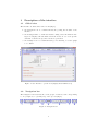
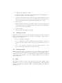
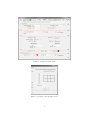
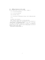
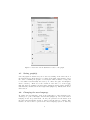
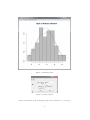
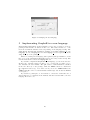
Introduction to GrapheR
Maxime Hervé
For any question, comment or suggestion: [email protected]
Thanks to Juan Alberti for the Spanish translation of the interface.
Thanks to Helmut Schlumprecht for the German translation of the interface
and the user manual.
1
Introduction
GrapheR is a multiplatform (Linux, Mac OS, Windows) user interface for drawing highly customizable graphs in R. It aims to be a valuable help to quickly
draw publishable graphs without knowing any R commands.
Six kinds of graph are available:
• histogram
• box-and-whisker plot
• bar plot
• pie chart
• curve
• scatter plot
GrapheR was built on the tcltk package, and consequently bugs can happen if R is configured in the MDI (Multiple-Document Interface) mode. It is
recommended to configure it in SDI (Single-Document Interface) mode before
starting the package.
GrapheR needs to function at least the 2.10 version of R and one additional
package: tcltk. Under Mac OS X, Tcl/Tk must have already been installed
(for more information see here).
2
Launching the interface
As with any other package, GrapheR is loaded via library(GrapheR), require(
GrapheR) or the Packages menu of the Windows R GUI. At this time, the tcltk
package is automatically loaded.
Launching the interface is the only step that requires the user to enter a
command: run.GrapheR(). The interface opens and the console can now be
reduced.
1
3
Description of the interface
3.1
Global view
The interface is divided into three blocks (Fig 1):
1. the navigation bar: it contains all buttons opening the modules of the
interface
2. the messages frame: to make the interface using easier, information messages are displayed in this frame when the mouse is over some specific
elements or when some specific actions are performed
3. the settings block: it contains all dialog boxes allowing to set the graph
to be drawn.
Figure 1: User interface – global view (display under Windows 7)
3.2
Navigation bar
The navigation bar is divided into seven groups of buttons, each corresponding
to one (obligatory or optional) step of the process (Fig 2):
Figure 2: Navigation bar
2
1. loading and modifying the dataset
2. setting up a graph. From left to right: histogram, box-and-whisker plot,
bar plot, pie chart, curve and scatter plot
3. opening a new graphics device: when a graph is drawn, it is in the active
window or in a new device if none is open. This button allows the user to
open a new graphics device in which several graphs can be drawn
4. draw a graph
5. adding elements to the graph. From left to right: add a horizontal line, add
a vertical line, add any other kind of line, add a theoretical distribution
curve, add text and add p-values
6. saving graph(s)
7. diverse options: user language and help.
3.3
Messages frame
When the mouse is over some specific elements of the GUI or when some specific
actions are performed, messages are displayed in this frame. Three kinds of
message can be displayed:
• in blue: informative messages
• in green: warnings, for when a particular attention should be payed to a
specific point (for example: if this option is chosen, then this one can not
be)
• in red: error messages, for when the action requested can not be completed. The message indicates the origin of the error.
3.4
Settings block
This block is divided into for to six sub-blocks, each containing options relating
to a given theme: general parameters of the graph, title of the graph, legend. . .
Each sub-block can be opened or closed with the corresponding arrow situated
on the right of the interface. Of course, defined settings are not lost when a
sub-block is closed.
4
Use
The example used here is based on the dataset provided in the package, called
Swallows. To load it, use the command data(Swallows). This (fictional!)
dataset exemplifies the legendary puzzle of African and European swallows’
migrations.
3
4.1
Loading and modifying the dataset
The first sub-block (Figure 3) allows you to load the dataset. Data can be
imported from an external file (txt and csv extensions are available so far) or
can be an already existing R object of class data.frame (i.e. a table).
The next sub-block allows you to get information on the dataset structure.
When a variable is selected in the list on the left, its type (numeric, factor,
logical. . . ) and its summary are displayed in the frame on the right.
The two next sub-blocks allow the dataset to be modified if needed:
• by renaming variables (for example if the dataset does not contain their
names)
• by converting variables into factors. The conversion can be applied to
variables of class character (i.e. characters chains vectors) or to numeric
variables (in this case values can be grouped into classes). The latter
case is necessary when a factor is numerically coded, e.g. a binary factors
(0/1), otherwise R would treat it as a numeric variable.
4.2
Setting up a graph
Once the dataset is ready, click on the button corresponding to the type of
graph to be drawn (histogram, box-and-whisker plot, bar plot, pie chart, curve
or scatter plot).
Whatever the type of graph chosen, all parameters have a default value
except general parameters – which correspond to variable(s) to be represented.
Hence, to quickly draw a graph, only general parameters must be defined. If
they are not (or not all) defined, an error occurs when trying to draw the graph.
Here the aim is to draw a histogram displaying the distribution of the size
of African swallows. We start by clicking on the Histogram button. In the
general parameters, we choose Size as the variable to be represented, and add
that we want to retain only the values corresponding to the African level of the
Species factor (Figure 4). The histogram type is set to densities, because
as the warning says only this type allows to draw the distribution curve of the
data.
All other settings are let to their default values, except the title of the graph
and those corresponding to the distribution curve (we tick Draw the curve and
define a color and a line type).
Once all necessary parameters are set, the graph is drawn by clicking on the
DRAW button of the navigation bar. At this time, you can choose to save the
code producing your graph in an external R file. If you answer Yes, code of all
graphs drawn in the same session will be added into this file.
If a new graphics device have to be beforehand opened, click first on the
window button (see next section).
4.3
Opening a new graphics device
It is possible to draw graphs in different windows and/or to draw several graphs
in the same one. To do this click on the window button of the navigation bar.
The dialog box that opens on the right of the interface allows specification of the
4
Figure 3: Loading the dataset
number of graphs to be drawn in the device to be created, and the background
color of this device (Figure 5).
It is possible to draw up to 16 graphs in the same device, shared between
four rows and four columns. However, the larger the number of graphs to be
drawn, the smaller the space allocated to each.
5
Figure 4: Setting up a histogram
Figure 5: Opening a new graphics device
6
4.4
Adding elements to the graph
Once the graph is drawn, elements can be added to complete it:
• one or several horizontal line(s)
• one or several vertical line(s)
• any other kind of line(s)
• one or several theoretical distribution curve(s): only on density histograms
• text
• p-values: only on bar plots.
These elements are always added to the last graph drawn.
For each element, clicking on the corresponding button in the navigation bar
opens a dialog box on the right of the interface.
Here we want to add a distribution curve to the histogram, corresponding
to the values of a normal law of parameters µ = 15.8 and σ = 2.2 (parameters
calculated from the data). Setting the curve is simple (Figure 6). Once all
settings are defined, click on Draw.
The graph is now finished (Figure 7).
7
Figure 6: Add a theoretical distribution curve to the graph
4.5
Saving graph(s)
Once all graphs are drawn, they can be saved by clicking on the save button of
the navigation bar. In the dialog box opening on the right of the interface, select
the device containing the graph to be saved (the window number corresponds
to the number automatically allocated by R, under the guise “R Graphics:
Device number ”). Then choose the extension of the file to be created (jpg,
png and tiff are available) and the image length (in pixels). Image height is
automatically calculated from the length value (Figure 8). Finally click on the
Save button.
4.6
Changing the user language
To change the user language, click on the lang button of the navigation bar.
A dialog box opens on the right of the interface (Figure 9). Choose the desired
language in the drop-down menu. To fix your preference in the future, tick
the Save the preference checkbox. Click on the Ok button to validate. The
interface is closed and re-opened in the chosen language (but note that any
8
Figure 7: Final histogram
Figure 8: Saving a graph
dataset loaded in the previous language session is lost and has to be re-loaded).
9
Figure 9: Changing the user language
5
Implementing GrapheR in a new language
Implementing GrapheR in another language is very easy, because no word appearing in the interface is written in the code. The button names etc. come
from an external file which is loaded depending on the language setting. English, French, German and Spanish are available so far (files Language en.csv,
Language fr.csv, Language de.csv and Language es.csv respectively, in the
lang directory of the package).
Therefore, adding a new language just requires a (strict) translation of each
line of one of the existing files (including spaces before and/or after words). The
new file must then be saved as Language XX.csv.
If you want to implement GrapheR in your language, you are most welcome.
In that case, remember that it would be a good idea (but a tougher job) to
also translate the user manual. The pdf version of this manual is contained
in the doc directory of the package, while the LATEX version is contained in
the vignettes directory). Note that even if you are not LATEX-familiar, the
LATEX-format file can be red and translated with script editors such as Tinn-R
or Notepad++.
If you want to participate, do not hesitate to contact me. I will take care of
all screenshots to be included in the manual, and then add the link to the new
language file in the code.
10