Download QuickStart guide

QUICK START GUIDE TO
COMPUTATIONAL PROTEIN DESIGN USING
COST FUNCTION NETWORK (CFN)
This document has been produced as a companion to Traoré et. al. (2013) in Bioinformatics, to get
you started with using the CFN-based approach for CPD. It presents a detailed example of how to
apply the approach to predict the optimal sequence or a sub-optimal ensemble of sequences for a
protein design problem targeting stability enhancement. The goal of this example is to assist the
user in setting up and applying this new CPD framework for their own protein design problems.
For reviewers, we also included a “Very QuickStart” (see section VII) that avoids all problem
generation steps (requiring extensive installations: amber9, osprey 2.0 and therefore also MPIJava).
This is achieved by making available the energy matrices computed by osprey for all 35 CPD
problems in the paper, as well as their translation to the CFN “wcsp” format. Together with
Python translation scripts, this should allow for a painless reproduction of computational results.
Otherwise, the setup for performing this CPD approach can be devised in five main steps: (i)
Parameterization of molecular structural system; (ii) Selection of search sequence-conformation
space; (iii) Computation of pairwise energy terms; (iv) Optimization of sequence-conformations;
(v) Score refinement and statistical analysis of top-score models. The details of each step are
described below.
I.
ARCHIVE CONTENTS
The archive of the pipeline used to generate energetic models (based on a patched version of the
open source solver osprey 2.0), the conversion to CFN models (based on Perl scripts) and CFN
solving (based on the open source solver toulbar2) is available at the following address
http://genoweb.toulouse.inra.fr/~tschiex/CPD/SpeedUp.tgz. The example of protein design is in the
example.1MJC directory. It contains the following directories:
 osprey2: patched osprey 2.0 with MPIJava sources and classes, compiled with Sun/Oracle
Java7 64 bits compiler.
 bin: contains toulbar2 binary file and a binary file for sequence analysis
 conf_info: will contain sequence-conformation files
 dat: directory for interaction energy matrix files during computation
 dat.save: will contain the saved matrix file
 files: contains some intermediary files
 inp: amber, cplex and osprey input files
 patch: patch to be applied to the original osprey2.0 sources if required
 pdbs: generated structures from selected results
 scripts: scripts to setup input files and making some analysis
 postmin_ana: post-minimization and repacking directory
It is assumed that you have installed java, amber9 and that our patched version of osprey2.0 can be
executed. All executions are assumed to run under a 64 bits Linux system with a Bourne shell. If
you lack any of these software, intermediary files are also available in the archive for IMJC or the
Very QuickStart can be tried (section VII).
II.
PARAMETERIZATION OF MOLECULAR STRUCTURAL SYSTEMS
You need a protein structure to redesign. In the example described here, we choose to redesign the
“Cold-shock protein A from E. coli”. The crystal structure of this protein is available in the
Protein Data Bank (PDB id: 1MJC). After downloading the structure, ATOM records are extracted
from the 1MJC.pdb file and saved into the 1MJC_edited.pdb file. Missing heavy atoms in crystal
structures as well as hydrogen atoms are then added using the tleap module of the Amber 9. Here is
given an example of input tleap file to accomplish this task for the edited 1MJC structure
(1MJC_edited.pdb): tleap.inp file
source leaprc.ff 99SB
X = loadpdb 1MJC_edited.pdb
set default PBradii mbondi2
check X
saveamberparm X 1MJC.prmtop
quit
#The force field parameter to be used
#The edited pdb file
#Radii set to be used(minimization step)
1MJC.inpcrd
The command to run tleap is:
$AMBERHOME/exe/tleap -f inp/tleap.in
Note that the environment variable $AMBERHOME must be set to point to the home directory of
the amber package.
For visual inspection of the structure, a pdb file (1MJC.hbuild.pdb) can be generated using the
following command:
$AMBERHOME/exe/ambpdb -pqr -p 1MJC.prmtop
-aatm
<
1MJC.inpcrd >
1MJC.hbuild.pdb
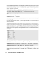
Finally, the molecular system is subjected to 500 steps of minimizations with the sander module of
Amber 9 (Case D. A. et al., 2006), using the Generalized Born/Surface Area (GB/SA) implicit
solvent model (Hawkins et al., 1996). A harmonic constraint with force constraint of 1 kcal.mol -1 is
applied to heavy atoms during this step in order to remain close to the starting conformation.
Underneath is given the input script used to perform this task with the sander module of amber9:
imin.inp file.
Initial minimization
&cntrl
imin
= 1,
maxcyc
= 500,
ncyc
= 250,
ntb
= 0,
igb
= 7,
rbornstat
= 1,
gbsa
= 1,
intdiel
= 4.0,
cut
= 12,
ntr
= 1,
restraint_wt = 1.0,
restraintmask = '!@H='
/
The commands for running the minimization step, followed by the generation of the resulting
structure are:
$AMBERHOME/exe/sander -O -i imin.inp -o 1MJC.min.out -c
-r 1MJC.restrt -ref 1MJC.inpcrd
$AMBERHOME/exe/ambpdb -pqr -p 1MJC.prmtop -aatm
1MJC.inpcrd
-p 1MJC.prmtop
<1MJC.restrt> model.pdb
The minimized structure (model.pdb) can be visualized using pymol (Schrödinger, 2010) for
example. After checking the minimized structural model, we can address the definition of
mutation space using a metric based on the residue depth in the molecule (its distance from
solvent).
III.
SELECTION OF SEQUENCE-CONFORMATION SPACE
Next, it is necessary to determine which residues to mutate and which ones to repack as well as the
amino acid type to be considered at each mutable position. 3 mutable residues (residues 17, 19 and
30) are selected in this example (1MJC). Allowed mutations at these selected positions depend on
the burial of residues within the protein. Residues are classified as core, boundary or surface
according to their solvation radius (see methods Traore et al, Bioinformatics 2013). For this purpose,
the atomic radii set included in the last column of the structure file (model.pdb) is used.
According to this stratification, the amino acids residues 19 and 30 are then classified into the core
layer while the residue 17 is defined in the boundary layer.
Mutable residues in the core (residues 19 and 30) are allowed to mutate to hydrophobic amino acids
(V,L,I,F,M,Y,W), boundary residues (residue 17) to hydrophilic amino acids (S,T,D,N,E,Q,H,K,R)
and surface residues (no residue in this example) to both sets. In addition, the alanine type and the
wild-type residue are considered at all mutable positions. The others residues of the core and the
boundary regions (residues 4, 5, 7, 8, 10, 11, 20, 21, 23, 28, 29, 31, 32, 33, 36, 43, 44, 48, 50, 51, 52, 53, 54,
66 and 67) are enabled to repack (i.e., flexible residues) in order to allow structural rearrangements
around mutable residues.
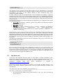
Below is given the command to accomplish the above tasks as well as the generation of
configuration files required to compute the pairwise energy matrix using osprey2.0 (see osprey2.0
user manual for further details).
./scripts/Config_mutation_space.pl inp/model.pdb inp/plist
The file plist contains the list of mutable residues:
17 LAYER
19 LAYER
30 LAYER
The configuration files generated in the inp directory are:



IV.
System.cfg: information about the protein system being redesigned
KStar.cfg: force field parameters and rotamer file specification
DEE.cfg: parameters for energy matrix and DEE/A* computations
COMPUTATION OF PAIRWISE ENERGY TERMS
This stage consists of the pairwise energy terms computation and the generation of the
corresponding matrix in text format (what is required to build CFN models). This is achieved
using osprey 2.0 (Chen et al., 2009; Gainza et al., 2013). You should try the patched an d compiled
version available in the Osprey2.0 directory which should work under most 64 bits Linux systems
with Java (6 or above) installed. If not, please look to the Appendix to, patch and compile Osprey
2.0 yourself.
The command lines for computing pairwise energy matrices are:
java -cp Osprey2.0/src:Osprey2.0/src/mpiJava/lib/classes -Xmx2G KStar -t 5 –c
inp/KStar.cfg computeEmats inp/System.cfg inp/DEE.cfg >matrix.out 2>&1 < /dev/null
The single and pairs interaction matrix files are saved into the ‘dat’ directory. These generated text
matrices
have to be concatenated into
a single text matrix (called
1MJC.matrix.28p.17aa.usingEref.txt) which is then used to generate the input file for toulbar2.
The following command line performs the concatenation and saves the combined text matrix
into dat.save directory.
./scripts/concat_pairwise_matrix.sh dat.save
V.
SEQUENCE -CONFORMATION OPTIMIZATION
The CFN-based optimization using toulbar2 is performed by scripts/CFN.sh.
./scripts/CFN.sh 1MJC.matrix.28p.17aa.usingEref.txt
This script involves the following steps:
1)
The translation of the pairwise matrix to the CFN ‘wcsp’ format:
mat=1MJC.matrix.28p.17aa.usingEref.txt # name of the matrix file
./scripts/mat2wcsp.pl –mat $mat -mwcsp -minself >make_wcsp.out
Where –mwcsp is a flag for translating to the CFN ‘wcsp’ format and –minself specifies the use of
reference
energy.
The
script
creates
the
input
for
toulbar2:
1MJC.matrix.28p.17aa.usingEref_self_digit8.wcsp
2) The computation of the GMEC (followed by the extraction of the solution from the output
and the translation of the costs into energy values).
name=1MJC.matrix.28p.17aa.usingEref_self_digit8
./bin/toulbar2 $name.wcsp –l=3 -m -d: –s > $name.wcsp.out
grep -A 1 "New solution" $name.wcsp.out|tail -1 > $name.wcsp.sol
./scripts/mat2wcsp.pl -mat $mat -minself -tb2sol $name.wcsp.sol > $name.wcsp.gmec.out
The file $name.wcsp.sol contains the solutions found by toulbar2 and $name.wcsp.gmec.out
contains corresponding energies (translation of unary and binary costs into kcal.mol -1 and the
corresponding total energy).
3)
The computation of sub-optimal ensemble (the cost of the GMEC is used to enumerate suboptimal solutions within some threshold from the GMEC energy (2 kcal.mol -1))
ew=$(( 2 * 10 ** 8 )) # 2kcal.mol-1
lb=`egrep "^Optimum:" ${name}.wcsp.out|awk '{print $2}'` # lowerbound
ub=$(( $lb + $ew )) # upperbound
./bin/toulbar2 $name.wcsp -d: -a -s -ub=$ub >$name.wcsp.enum 2>&1
4) Solutions from $name.wcsp.enum are extracted, sorted and translated into osprey format using
the following command line:
./scripts/simple_ana.sh $mat
VI.
SCORE REFINEMENT AND STATISTICAL ANALYSIS OF TOP-SCORE MODELS
First, from the enumerated sub-optimal sequence-conformation models, the unique sequences are
extracted and their occurrences are determined. This task is performed by the simple_ana.sh script
and the result file is $name.wcsp.enum.res.ana. A fasta format file is also generated from these
unique sequences, and Weblogo (Crooks et al., 2004) can be used to visualize the propensity of each
amino acid type at each mutable position.
Second, in order to evaluate the effect of the relaxation of side-chains and backbone degrees of
freedom of the best conformation for each unique sequence on the energy ranking, energy
minimization and rescoring steps are carried out as well as the number of conformation accessible
to each mutant within some threshold (0.2 kcal.mol -1 here).
The extraction of unique sequences (best conformation) and structure building using osprey is
performed by scripts/GenStruct.sh.
The tleap module of amber9 is used to produce the .inpcrd file of the generated models which are
then subjected to energy minimizations using the sander module of amber9. In this example,
1000 steps of minimizations are performed using the Generalized Born/Surface Area (GB/SA)
implicit solvent model (Hawkins et al., 1996). Here is the command line for the generation of
amber input files and the minimization of unique sequence structures:
./scripts/amberin.pl
./scripts/amber-postmin.sh
The amberin.pl script generates all input files required for the minimization of all selected
conformations (best conformation per sequence) while the amber-postmin.sh script performs the
minimization. The energy of the refined structure is then reevaluated using osprey
(computeEnergyMol command).
In order to assess the effect of the minimization on the conformational variability, a repacking
optimization can be carried out on the minimized structures. This is accomplished by performing
a matrix computation using osprey and sub-optimal enumeration using CFN-based approach with
some initEw value (0.2 for example) for each of the unique sequences. These tasks are performed by
run_post_ana.sh.
Here is given the description of some modifications accomplished in the configuration files of each
of the unique sequences:
 System.cfg: the parameter “pdbName” points to the pdb file of the minimized structure
of the considered sequence.
 KStar.cfg: unchanged.
 DEE.cfg: the “initEw” parameter is set to 0.2; all lines “resAllowed” are deleted; the
“minEnergyMatrixName”,
“erefMatrixName”
and
“maxEnergyMatrixName”
parameters should have a different name for each sequence; parameter “AddWTRots” and
“AddWT” are set to true.
In the directory postmin_ana, each sequence has its own subdirectory because text matrices are
written into the dat sub-directory. For each sequence, the matrix computation and CFN
optimization are identical to the process defined above, except that the reference energy is not used
during the optimization step since each sequence is optimized independently (flag –minself is not
used). Also notice that if you just need the number of conformation within initEw, the flag ‘-s’ can
be omitted.
The following command lines perform the matrix computation using osprey as well as the CFNbased repacking using toulbar2:
./scripts/run_post_ana.sh
cd postmin_ana
./run_mutantMatrices.sh
./run_mutantPostCFN.sh
For the rescoring and the energy matrix computation, the script run_post_ana.sh generates two
files for each mutant computeMats.sh and PostMinCFN.sh. The first one reevaluates the energy of
the minimized structures and the second one carries out the repacking. The computation for all
mutants can directly be performed using run_mutantMatrices.sh (applies all computeMats.sh) and
run_mutantPostCFN.sh (applies all PostMinCFN.sh).
VII.
VERY QUICK START
To be able to just reproduce the main results w/o major efforts or software installation, please
download the energy matrices produced by osprey 2.0 and their translated version to the “wcsp”
format the problems considered in the paper. Each file, compressed with the strong “xz”
compressor,
(available
under
most
Linux
distributions)
is
available
at
http://genoweb.toulouse.inra.fr/~tschiex/CPD.
Download and extract the wcsp file of the problem of your choice (the 1MJC instance is used
below) in the example directory (please be sure to have the required disk space available) and
uncompress it:
unxz 1MJC.matrix.28p.17aa.usingEref_self_digit8.wcsp.xz
This creates (a possibly large) .wcsp file for toulbar2.
 You can identify the GMEC using toulbar2 directly on the “wcsp” files as described in
section V (item 2).

You can enumerate all solutions within 2 kcal/mol of the GMEC using toulbar2 directly
on the wcsp files, once the GMEC has been identified and stored above. Just follow Section
V, item 3.
For testing the ILP approach, notice that IBM ILOG cplex is free for academics. You must contact
the IBM academic initiative to be able to download and install the cplex software. Please proceed as
described on the dedicated IBM academic initiative web site at http://www01.ibm.com/software/websphere/products/optimization/academic-initiative/.
You can then translate any of the “wcsp” files to the cplex “lp” format using the wcsp2cplex.py 1
scripts:
./scripts/wcsp2cplex.py 1MJC.matrix.28p.17aa.usingEref_self_digit8.wcsp > 1MJC.lp
Under cplex command line interface, you can identify the GMEC with the following
commands:
read 1MJC.lp
read inp/cplex.prm
optimize
write 1MJC.sol
REFERENCES
Case D. A. et al. (2006) AMBER 9 University of California, San Francisco.
Chen,C.-Y. et al. (2009) Computational structure-based redesign of enzyme activity. Proceedings of the National
Academy of Sciences, 106, 3764–3769.
Crooks,G.E. et al. (2004) WebLogo: a sequence logo generator. Genome Res., 14, 1188–1190.
Gainza,P. et al. (2013) osprey: Protein Design with Ensembles, Flexibility, and Provable Algorithms. Meth.
Enzymol., 523, 87–107.
Hawkins,G.D. et al. (1996) J. Phys. Chem., 100, 19824.
Schrödinger,L. (2010) The PyMOL Molecular Graphics System, Version 1.3r1.
1
Although this is not described in this paper, for curiosity, other Python scripts (wcsp2qp.py, wcsp2sat.py,
wcsp2sat-support.py) are provided in the “scripts” directory to translate to cplex Quadratic Programming
format, and to MaxSAT (with two different encodings).
VIII.
APPENDIX : INSTALLING AND PATCHING OSPREY 2.0
This is required only if the patched provided version in Osprey2.0 directory does not work on your
system. You can download the Java sources of osprey 2.0 from the following web site:
http://www.cs.duke.edu/donaldlab/software/osprey/request_download.html
Once extracted, the files to patch are in the src directory of the osprey 2.0 installation directory (the
path to this directory is assumed to be available in the $OSPREYHOME environnement variable).
patch $OSPREYHOME/src/RotamerSearch.java < patch/RotamerSearch.patch
patch $OSPREYHOME/KSParser.java < patch/KSParser.patch
Then recompile osprey (the MPIJava library must be available too, see Osprey documentation):
javac –cp mpiJava/lib/classes $OSPREYHOME/src/*.java