Download SpikePac User`s Guide - Tucker

SpikePac User’s Guide
Updated: 7/22/2014
SpikePac User's Guide
Copyright
© 2008-2014 Tucker-Davis Technologies, Inc. (TDT). All rights reserved.
No part of this manual may be reproduced or transmitted in any form or by any means, electronic
or mechanical, including photocopying and recording, for any purpose without the express written
permission of TDT.
Licenses and Trademarks
Windows 7 is a registered trademark of Microsoft Corporation.
ii
Table of Contents
BEFORE YOU BEGIN ................................................................................................................................ 1
SOFTWARE REQUIREMENTS ........................................................................................................................ 1
HARDWARE REQUIREMENTS ....................................................................................................................... 1
INSTALLATION ............................................................................................................................................ 1
OPENEX FUNDAMENTALS ........................................................................................................................... 1
ORGANIZATION OF THE MANUAL ................................................................................................................ 1
INTRODUCTION ........................................................................................................................................ 3
THE TOOLS ................................................................................................................................................. 5
OVERVIEW .................................................................................................................................................. 5
SpikePac Macros .................................................................................................................................... 5
The Controls ........................................................................................................................................... 6
PCSORT - PRINCIPAL COMPONENT FEATURE SPACE SPIKE SORTING .......................................................... 7
BOXSORT - TIME-VOLTAGE SPIKE SORTING ..............................................................................................23
TETSORT - TETRODE SPIKE SORTING .........................................................................................................36
TetSort Control Window ........................................................................................................................37
Selecting the Active Tetrode ..................................................................................................................38
Adjusting the Detection Threshold ........................................................................................................38
Working with the Plots ..........................................................................................................................39
Hunt Mode .............................................................................................................................................42
Sorting in the Active Tetrode Plot Display ............................................................................................44
The Setup Properties .............................................................................................................................52
Tool Buttons ..........................................................................................................................................55
IZ2STIMGEN – STIMULUS GENERATION ....................................................................................................58
The Buttons ............................................................................................................................................59
iii
SpikePac User’s Guide
Burst Display Graph..............................................................................................................................60
Designing the Stimulus ..........................................................................................................................60
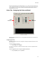
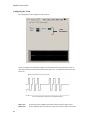
Voice Tab – Designing the Pulse and Burst ..........................................................................................61
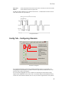
Config Tab – Configuring Channels......................................................................................................65
Impedance Tab ......................................................................................................................................67
NEUROFILTER - FILTERING ........................................................................................................................69
NEUROMON - SIGNAL MONITORING WITH NOISE GATING .........................................................................70
SITEMAP - ELECTRODE SITE REMAPPING...................................................................................................72
TUTORIAL ..................................................................................................................................................75
ONLINE SPIKE SORTING WITH SPIKEPAC ....................................................................................................75
Planning the Project ..............................................................................................................................75
Setting-Up Your Hardware....................................................................................................................76
Creating the Project ..............................................................................................................................76
Creating the Circuit File .......................................................................................................................78
Build the OpenWorkbench Experiment .................................................................................................85
Adding the Real-time Controls ..............................................................................................................89
Running the Experiment ........................................................................................................................91
Stopping the Experiment........................................................................................................................93
Wrapping Things Up .............................................................................................................................94
What's Next? ..........................................................................................................................................94
GLOSSARY .................................................................................................................................................95
KEYBOARD SHORTCUTS ......................................................................................................................96
REFERENCES ............................................................................................................................................97
iv
Before You Begin
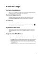
Software Requirements
TDT Drivers and the OpenEx Software Suite must be installed before installing SpikePac. The
recommended operating system for all TDT systems is Windows 7®.
Hardware Requirements
The SpikePac tools are supported by RX or RZ System 3 High Performance Processors.
See the System 3 Installation Guide for hardware installation and set-up instructions.
Installation
Install TDT Drivers and OpenEx prior to SpikePac.
Installing SpikePac enables special features in OpenEx and RPvdsEx, notably, adding an
Insert SpikePac Macro button to the RPvdsEx toolbars.
OpenEx Fundamentals
SpikePac builds on existing features in the OpenEx Suite. TDT recommends completing the
Getting Started in OpenEx Tutorial found in the OpenEx User Guide before working with
SpikePac.
Organization of the Manual
This manual is organized in the following sections:

Introduction: A brief overview of the SpikePac tools and how they work with OpenEx.

The Tools: A guide for the SpikePac Macros and control sets provided by SpikePac.

Tutorial: A step-by-step tutorial for building an OpenEx Project using SpikePac Macros.

Glossary: A listing of the terms associated with this user guide and their definition.

Keyboard Shortcuts: A useful reference to the various shortcut keys used for viewing
and working with data.

References: A listing of the sources that may be referenced for additional information.
1
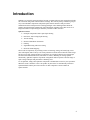
Introduction
SpikePac is a powerful extension package for TDT’s OpenEx software suite designed specifically
for researchers doing multi-channel neural recordings. The software package includes a group of
easy-to-use RPvdsEx components and paired OpenController interfaces that provide the
foundation needed to build powerful recording paradigms. These building blocks handle all
OpenEx integration details automatically. Most importantly, SpikePac offers this new level of
integration without compromising the flexibility essential to TDT customers.
SpikePac includes:

Principal Component Feature Space Spike Sorting

Real-Time, Time-Voltage Spike Sorting

Tetrode Sorting

Electrical Stimulation Generation

Filtering

Signal Monitoring with Noise Gating

Electrode Site Remapping
These tools focus primarily on providing a means of detecting, storing, and classifying events
(also called spikes) that are likely to be action potential waveforms that result from neural firings.
The process of spike sorting attempts to separate the waveforms into distinct waveform groups
associated with individual neurons (called units or clusters). Building on existing OpenEx
functionality, SpikePac simplifies experiment configuration and incorporates a broader range of
spike sorting techniques and performance enhancing tools.
To use SpikePac, simply add a SpikePac component to the RPvdsEx circuit for your experiment.
When the circuit is loaded to a device in OpenEx any data stores are automatically inferred in
OpenWorkbench and the paired user interface for that component is made available in
OpenController.
3
SpikePac User’s Guide
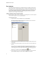
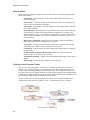
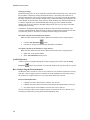
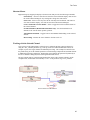
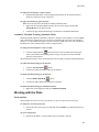
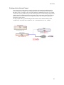
The diagram below illustrates the experiment design process, highlighting the automation
provided by SpikePac.
SpikePac Process Flow Chart
User Controlled
Processes
Configuration
Information
from Circuit
Design the Circuit in RPvdsEx
SpikePac macros generate
automation information
Assign the circuit to a processor in
OpenWorkbench
Data
Configure OpenWorkbench
Data Stores autodetected
Configure OpenController
Control sets autoconfigured
Run Protocol in OpenWorkbench
Adjust real-time controls in
OpenController
Data Tank time stamps and stores data
4
The Tools
Overview
SpikePac Macros
When OpenWorkbench hardware server loads a circuit containing a SpikePac macro to a
processor, the OpenController client will make the corresponding control available to the user.
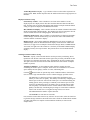
Macro Configuration
Macro configuration options are accessed through the macro setup dialog menu. Double-clicking
on any macro will open the setup properties dialog menu and onboard help.
ID
IDs are used to identify the corresponding data stores and parameters that can be controlled via the
runtime application. The ID is automatically appended to the end of the name of the corresponding
OpenController control set and ensures that all parameter targets are found and enabled for realtime control. Users must ensure that any two instances of the same macro are assigned unique IDs.
That is, if a NeuroFilter and a NeuroMon macro are added they may share the same ID. If a
second NeuroFilter macro is added it must use a different ID.
Note: Store Pooled macros share the same ID and Store names. See the PCSort or BoxSort
onboard macro help for more information about store pooling.
Parameter Summary
As shown above, the macro parameter summary displays the ID and other macro information,
such as data Stores.
Adding a SpikePac Macro in RPvdsEx
SpikePac macros are added to circuits in much the same way as existing macros and offer the
same easy-to-use parameter setup dialog box.
To quickly add a SpikePac macro:

In RPvdsEx, click the
then click the workspace.
Insert SpikePac Macro button and select the desired macro
See the Tutorial: Online Spike Sorting with SpikePac, page 75, for step-by-step practice with
incorporating SpikePac Macros into your circuit design.
5
SpikePac User’s Guide
The Controls
The controls provided by SpikePac are pre-configured control sets for higher level tasks such as
filtering, spike-sorting, or channel-monitoring. They are available in OpenController only when
the compiled circuit file loaded through OpenWorkbench contains the corresponding macro. For
example, adding a SpikePac filtering macro to an RPvdsEx circuit will allow a pre-configured
filter control to be added in OpenController design mode. SpikePac controls save time and
eliminate the need to configure controls manually.
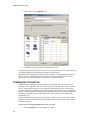
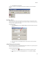
Adding a SpikePac Control in OpenController
Before attempting to add the control, ensure that the corresponding macro is used in the compiled
circuit file that is assigned to a device in OpenWorkbench.
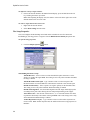
To quickly add the Control:
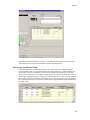
1.
In OpenController, click the Controls menu, select Power Macro.
The Controls dialog box displays a list of controls available and a list of controls that
have already been added to OpenController.
2.
Select the desired control and click OK. The pointer changes to indicate that the control
can be added.
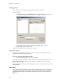
3.
Click the grid to position the upper-left corner of the control. The control is added to the
grid area.
These controls are pre-configured and initialized using information in the compiled
circuit file, so they can usually be used without any additional configuration. If you need
to make changes to the control, double-click the control to display the setup properties
dialog box (or, if available, click the Setup Properties
4.
6
button).
Before running the control, the corresponding OpenWorkbench file must be open and a
protocol should be running. To run the control, click Run! on the menu bar.
The Tools
PCSort - Principal Component Feature Space
Spike Sorting
PCSort
Store (nChan=16)
SortCode
ID: Neu, Store: 'eNeu/pNeu'
The PCSort macro is used to time stamp and store waveform events as data snippets. It supports
online spike sorting through the PCSort control in OpenController. Candidate waveforms are
detected based on their deviation from the noise of the system. By default, the time stamp and
position of the waveform in the snippet is dependent on the time of the threshold crossing for the
signal. An alternative setting allows waveform time stamp and positioning to be determined by the
waveform’s highest peak, aligning snippets to their respective peaks. The macro can be configured
to output the sort code for each channel once sorting parameters have been loaded to the hardware
through OpenController.
This macro generates two data Stores: one for sorted snippet data, designated with the prefix e,
and one for the plot decimated data stream (a representation of the waveform using maximum and
minimum values and used to visualize spike activity), designated with the prefix p. The ID is
appended to the Store names and both are displayed in the macro’s parameter summary.
Settings for configuring the number of channels, threshold mode, number of clusters and spheres,
and window width for each snippet stored are defined in the macro properties dialog box. See the
onboard help for more information.
The corresponding PCSort control set works in three general phases:
Training
When run, the control set implements spike detection and a training time begins. Events collected
during the training time are used to calculate the feature space. By default, auto-clustering is
disabled and no clustering (or sorting) takes place until initiated by the user.
Classification
The next phase begins when clustering is initiated. Preliminary identification of units is indicated
by color coding in the control’s displays for visualization; however, all candidate spikes are saved
to the data tank with a sort code of 0 during this phase. The default clustering method is a
Bayesian algorithm, but users may choose a K-means method or edit clustering using manual
cluster cutting techniques. During this phase the user can explore the data and modify sort
parameters without affecting saved data.
Sorting
When satisfied with the clustering, the user can choose to Apply Sorts. The clustering parameters
are loaded to the circuit running on the hardware and sort codes will be applied to new data as it is
acquired in real-time.
The default threshold factor, peak alignment, training termination control, sorting algorithm, and
auto-clustering are modified by the user in the control’s Setup Properties.
7
SpikePac User’s Guide
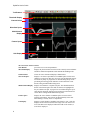
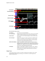
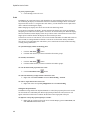
Tool Buttons
Threshold Display
Channel Select
Waveform Space
Multi-Channel
Display
Feature Space
Unit Display
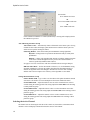
The Control Set window includes:
8
Tool Buttons
provide access to tools and parameters.
Threshold Display
displays the plot decimated waveform of the currently selected channel
and allows threshold adjustments under manual thresholding mode.
Channel Select
selects the active channel and displays channel status.
Waveform Space
displays a waveform representation of candidate spikes for the active
channel in a pile plot. In this plot, users can view and manually classify
waveforms by shape. A progress bar is included along the top of the
plot during the training period. Indicators in the bottom left corner
denote scaling and threshold tracking states.
Multi-Channel Display
displays each channel in a separate sub-plot. The channel number is
shown in the bottom right corner and waveforms are highlighted as
they are added to the plot. A progress bar is included along the top of
each sub-plot during the training period. Indicators in the bottom left
corner denote scaling and threshold tracking states.
Feature Space
displays the active channel of candidate spikes in terms of their
principal components. This reduces the dimensionality of the data
while making it visually easier to comprehend.
Unit Display
displays a single channel of candidate waveforms by unit—each plot
displays all waveforms classified with a single sort code. If there are
more units than can be displayed within the width of the window, a
scroll bar is displayed.
The Tools
Simple Zoom
You can zoom any plot to see more or less detail. Zooming does not attempt to scale or fit the
waveform shape or data in the plot, allowing you to control the view without regard to the
limitations of the plot size.
Note: changing the zoom level in the Multi-Channel Display alters the zoom level for all channels
in the Multi-Channel Display.
To change the zoom level of any plot:

Point to the center of the plot, press and hold down the Shift key, and drag the mouse up
or down.
To reset the view of any individual plot:

Hold down the Shift key and double-click the mouse within the plot.
Note: this method can be used to reset the feature space to its default position.
Display Scale
When the PCSort control set is run, all channels begin at a base scale of 1. This type of scaling
clearly shows differences in magnitude across units but can make it more difficult to see
waveform shapes for some channels.
To make it easier to see waveform shapes for channels with lower magnitude, you may scale
individual channels manually or normalize all channels to fit to a similar scale. If you choose to
normalize the display, the PCSort control set calculates the display scale for each channel
individually, attempting to fit around 80% of the signal’s vertical size in each plot. In the case of
the Multi-Channel Display, the waveform with the largest magnitude is used to compute the fit.
When the display has been normalized, PCSort displays either an up or down arrow in the bottom
left corner of the plot or subplot to indicate whether the display has been scaled up or down.
An Auto Scale feature can be used to refresh the scale of plots either with or without normalizing
the display. Note: changing the display scale does not alter the data being stored.
To refresh the display without normalizing plots:
1.
Click the Auto Scale
button.
2.
Click No when asked if you want to normalize all window groups.
Note: this will not reset the feature space display.
To normalize all channels:
1.
Click the Auto Scale
button.
2.
Click Yes when asked if you want to normalize all window groups.
Note: an arrow will now be displayed on the bottom left corner (next to the threshold
mode indicator) which indicates positive or negative deviation from the base scale
setting.
To return all channels to their base scale:
1.
Click the Base Scale
2.
Click Yes.
button.
Note: resetting plots to base scale does not remove any Zoom applied to a plot.
9
SpikePac User’s Guide
To adjust the scale of a single channel:

Point to the desired channel in the Multi-Channel display, press and hold down the Ctrl
key, and drag the mouse up or down.
Note: while adjusting the display scale, the numeric value in the lower right corner of the
channel indicates the new scale value.
To return a single channel to its base scale:
1.
Right-click the desired channel.
2.
Select Reset Scaling from the menu.
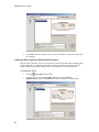
The Setup Properties
Users can configure the control, choose a Bayesian or K-mean sorting algorithm, and enable or
disable auto clustering in the control set’s Setup Properties.
To open the setup properties:

Click the Setup Properties
button.
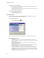
The Setup Properties window includes four parameter groups available from a drop down list.
Thresholding Parameter Group
Threshold Factor – Select a value to set base threshold for spike detection to a value
which is n * STD of the signal RMS. This setting is active only when automatic threshold
tracking is enabled.
Threshold Window Time Span – Type a numeric value to set the time span of the
threshold window in seconds.
Default Search Polarity – Select a positive or negative polarity for the threshold value.
This setting is active only when automatic threshold tracking is enabled.
Default Peak Alignment – Sets the default alignment to Peak Align which aligns spikes
according to their peak values altering the time stamp and positioning of the snippet.
Track Time Const – Sets the time constant tau to 3, 5, or 10 seconds. Shorter tau values
respond more drastically to deviations in the signal RMS value. This setting is active only
when automatic threshold tracking is enabled.
10
The Tools
Artifact Rejection Level (µV) – Type a numeric value to set the artifact rejection level
in micro Volts. Note: Artifact Rejection must be enabled in the macro setup properties in
RPvdsEx.
Display Parameter Group
Clear History Counter – Enter a number to set a limit on the number of events
displayed prior to a display refresh. This does not delete historical data from the data
tank. It simply removes existing data displays and refreshes each plot. With the default
setting of 0, plots will display accumulated historical data.
Max Channels To Display – Enter a number to limit the amount of channels that will be
displayed in the Multi-Channel Display. The channel select bar will reorganize into one
or more columns based on the settings applied. The default value is 64.
Channel Column Count – Enter a number to set the number of columns for the MultiChannel Display. With the default setting of 0, the PCSort control will automatically
select the number of columns to display.
Display Layout – Select either Standard or MultiChannel View modes of display. In
Standard display mode the Threshold and Unit displays extend the entire width of the
control set (see page 8 for an example of the Standard Display Mode). In MultiChannel
View mode, the right side of the control set is used only for the Multi-Channel Display,
extending vertically from top to bottom. This provides more room for multi-channel
display.
Training Control Parameter Group
Ref Tank – Specify a reference tank that the user has previously sorted using TDT’s
OpenSorter. The PCSort control will load an eigenvector previously calculated for that
sort and use it to determine the feature space, eliminating the need for a training time.
The spike event in the selected reference tank must have the same number of samples
(number of points).
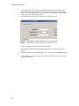
Training Termination – set the conditions under which the training period for
calculating the features space is complete. Three factors are considered: score (feature
space stability and sort quality), number of events, and training time.
Click the
Browse button to open the Stop Teach Condition window, which allows
users to create a logic statement that is used to evaluate and apply specified criteria.
The sort score is a value between 0 and 1 that reflects both feature space
stability as well as the sort quality. The stability is measured by comparing one
feature space to the next each time the feature space is recalculated during the
training period. As the percentage of variability in the feature space for each
successive calculation decreases, the feature space is considered more stable.
The sort quality is an indication of how well the defined clusters fit the data.
Quality is measured by considering the percentage of events that lie within the
clusters. The overall score is a weighted average of these two factors.
The event count is the number of spikes detected.
The teach time is a time interval in seconds.
First, enter the Greater Than value for any criteria to be used. Then, select the check box
to generate the logic statement. Selections in the same column are ANDed while columns
are ORed. This allows for complex teach termination conditions, as shown in the
example below.
11
SpikePac User’s Guide
Greater than:
Score AND Event Count
OR
Event Count AND Teach Time
OR
Score AND Teach Time
If all termination conditions are omitted (unchecked), a warning will be displayed after
the OK button is pressed.
Auto Clustering Parameter Group
Auto Cluster Active – Automatically clusters all channels as the feature space is being
calculated. This renders the display sphere button inactive until the feature space has
either been accepted or training has ended.
Clustering Method – Select between Bayesian and KMeans sorting algorithms.
Bayesian - Sorting based on expectation-maximization analysis of Bayesian
probabilities.
KMeans - A binary split algorithm that attempts to find the optimum locations
of the cluster centers through an iterative process and a defined number of
clusters (specified by KMeans Num Clusters).
See page 97 for a list of references with more information about sorting techniques.
KMeans Num Cluster – Set the max number of clusters (1-5) for the KMeans sorting
algorithm. If KMeans is selected, this number determines the maximum number of
clusters the algorithm will iterate through to find the best fit for the data. If adding
another cluster does not improve the efficiency of the algorithm it is not added.
Sorting Model Parameter Group
Cluster Radius xSTD – Type a value to set the radius of the sphere boundaries around
each cluster. The number is a factor multiplied to the cluster standard deviation.
SortTerminateTime – Adjust the numeric value to set the termination time value in
seconds during the training period. This setting adjusts the Teach Time in the Training
Control parameter group.
SortTerminateCount – Adjust the numeric value to set the termination count value
during the training period. This setting adjusts the Event Count in the Training Control
parameter group.
SortTerminateScore – Adjust the numeric value to set the termination score value
during the training period. This setting adjusts the Sort Score in the Training Control
parameter group.
Selecting the Active Channel
The channel selector bar along the left side of the control set (shown below) determines which
channel is active and displays information about the status of each channel.
12
The Tools
To set a channel as active:

Click the selector box for the desired channel.
The active channel is displayed in all single channel plots within the set
and is highlighted in the multi-channel plot.
Active Channel
Color is light blue.
Training Complete
Color is dark blue.
Locked Channel*
Color is gray.
*See Tool Buttons on page 20 for more information.
The color of the channel selector indicates the status of each channel. When training is active and
the feature space is being calculated, the colors will match the training progress bar. The selector
appears blue once the training is complete or if the feature space is accepted. If a channel is
locked, the color on the selector will be shown as gray. For more information about the training
period, see Calculating the Feature Space, page 16.
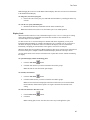
Using the Threshold Control
The threshold control displays the plot decimated waveform for the selected channel along with
the threshold marker. The default value specified for the threshold factor is 6.5 x STD (standard
deviations from the waveform’s RMS value).
To change the base threshold:

Click the Setup Properties
button and select a new Threshold Factor from the
Thresholding parameter group. You can also change the search polarity of the Threshold
in this parameter group. See page 10 for more threshold parameter setting options.
Note: base threshold values only affect threshold tracking.
Threshold Tracking
Threshold tracking adjusts the threshold in response to changes in each channel waveform’s RMS,
using a default time constant (tau) of five seconds.
13
SpikePac User’s Guide
Note: tracking is performed on the DSP and is enabled by default in the PCSort macro.
Automatically tracking the threshold on many channels of data can tax the processor; see Saving
Cycle Usage below if you are recording many channels.
When threshold tracking is active the threshold bar will be locked preventing manual adjustments.
An ‘A’ indicator is placed in the bottom left corner of the Waveform Space and Multi-Channel
Display plots to denote if threshold tracking is currently active for a given channel. Otherwise, an
‘M’ indicator will be shown to denote that threshold tracking is disabled.
Threshold tracking is active
for the current channel.
Threshold tracking is
disabled for the current
channel, allowing for
manual threshold
adjustments.
To enable threshold tracking for all channels:
Note: automatic threshold mode must be enabled in the PCSort macro setup properties.
1.
Click the Auto Threshold
button.
2.
Click Yes to enable threshold tracking for all channels.
To enable or disable threshold tracking for individual channels:

Right-click on the desired channel and select either Auto Threshold or Manual
Threshold.
To disable threshold tracking for all channels:
14
1.
Click the Manual Threshold
button.
2.
Click Yes to disable threshold tracking for all channels.
The Tools
Setting the Threshold Manually
When the corresponding channel is set to manual threshold mode, the threshold bar may be
adjusted manually in the threshold control window by clicking and dragging the threshold bar
(shown below).
Note: hold the Ctrl key and
double-click the Threshold
Display to toggle threshold
tracking on or off for the active
channel.
Manual adjustments to the threshold can also be made in the waveform space as shown below.
To change the threshold for a single channel:

Click and drag the threshold bar to the desired location in either the Waveform Space or
Threshold Control plots.
To apply the current threshold setting for all channels:
Note: this will only set the threshold for channels in which threshold tracking is disabled.
1.
Right-click the desired threshold location in the Threshold Display.
2.
Select Set Threshold Here from the menu.
3.
Click Yes to apply the threshold setting to all channels in manual threshold mode.
Saving Cycle Usage
Threshold tracking relies on circuit components contained within the PCSort macro. This means
that the DSP is continuously tracking the threshold while it is performing other tasks such as
filtering and acquisition. This process is taxing on the device cycle usage rates and may diminish
the ability of PCSort to process higher channel counts. Threshold tracking can be disabled in the
circuit through the PCSort macro setup properties. When disabled, only manual threshold mode is
available (signified by the manual threshold button being grayed out). Manual threshold methods
must be used to obtain the threshold settings but this frees up cycle usage on the DSP enabling
more processing.
In addition to disabling threshold tracking, the PCSort control alters the functionality of the
Automatic Threshold button. When the button is clicked, an instantaneous calculation of the data
is performed by the PC to determine a reasonable threshold setting for all channels.
15
SpikePac User’s Guide
To instantly calculate the threshold for all channels:
Note: automatic threshold mode must be disabled in the PCSort macro setup properties.
1.
Click the Auto Threshold
button.
2.
Click Yes to calculate the instantaneous threshold for all channels.
To instantly calculate the threshold for a single channel:
Note: automatic threshold mode must be disabled in the PCSort macro setup properties.
1.
Right-click the desired channel.
2.
Select Auto Threshold from the menu.
Artifact Rejection
Artifact rejection is configured through the control setup properties window using the Setup
Properties
button. Once enabled, events that fall outside of the specified value are ignored.
Calculating the Feature Space
When the control is run, a training period begins, during which the feature space is calculated. As
events are added to the control display they become part of the history or data set used for feature
space calculation. The feature space is periodically recalculated using all data in the history at that
time until the training period is complete.
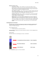
During the training period, a colored progress bar (shown above) is added to many of the plots. A
pointer moves along the bar to show progress towards the maximum time for training.
By default, the progress bar is colored blue. If active auto-clustering is enabled, the color of the
bar indicates the current score for the feature space.

Red = poor score

Yellow = good score

Green = great score
Arrows located on either end of the training progress bar can be used to restart the time variable of
the training period (left arrow) or to accept the feature space (right arrow) for the active channel.
The training period continues until one of the following two conditions is met:

The termination condition is satisfied (see page 11).

The feature space is manually accepted by the user.
When the training period is ended, automatic or manual clustering methods can be used.
To accept the current feature space for all channels manually:

16
Click the Accept Feature Space
button.
The Tools
To recalculate the feature space for all channels:

Click the Recalculate Feature Space
button.
When clicked and confirmed, this option will prompt you to either keep the existing event history
or clear it prior to recalculating the feature space.
To clear the event history:

Select Yes after selecting Yes to recalculate the feature space.
or

Right-click a plot for the desired channel, click Clear History on the shortcut menu.
or

Click the Clear All History button
and select Yes.
Note: clearing the event history will not affect waveforms stored to the data tank.
Calculating Clusters Automatically
When the user is satisfied with the feature space, clusters can be calculated.
To calculate clusters for all channels:

Click the Calculate Clusters button
and click Yes when asked to confirm.
The algorithm and options in the set-up properties are used to calculate clusters automatically.
If the training time has not yet been completed, calculating clusters will terminate training
accepting the current feature space.
Once clustering begins, each sort code (or “unit”) is represented by a single color for all plots.
Applying Sorts to New Data
Sort codes are not saved to the data tank until sorts are applied by the user. You can re-sort or
make adjustments as needed to get the best results.
To begin saving sort codes to the data tank:

Click the Apply Sorts
button.
Sort codes are applied as new data is acquired. Once sorts have been applied, any changes in
sorting parameters in the display will be applied automatically.
Note: at this time, if the sort code output is enabled in the macro setup properties, the SortCode
output of the macro will output the sort code values for each channel.
Viewing Events in the Feature Space Pane
In the feature space, waveforms can be viewed in terms of their principal components. This
automatically reduces the dimensionality of the data while making it visually easier to
comprehend.
17
SpikePac User’s Guide
To rotate the feature space:

Click the left mouse button and drag the feature space from the desired angle.
To pan the feature space:

Press and hold the Alt key on the keyboard and drag the mouse to pan the feature space.
To auto scale/reset the feature space:

Press and hold the Shift key on the keyboard and double-click the mouse anywhere in the
feature space.
Manually Assigning Events to a Cluster in the Feature Space Pane
Users can manually assign waveforms to clusters using mouse based selection tools. Manual
sorting can be used as the primary sorting method, however, it is more often used to edit and
reassign units after automated sorting.
To assign events to clusters manually:
1.
Press and hold the Ctrl key on the keyboard and use the mouse to draw an arbitrary
shape around a visible cluster.
When the mouse button is released, the Send Events To dialog opens. The dialog box
lists the available Sort Codes as well as the number of events currently sorted by each
Sort Code.
18
The Tools
2.
Select the desired Sort Code from the list or click the Next Empty Code button.
Defining Clusters Manually in the Waveform Space
The waveform space (shown below) displays waveform shapes for all events on the active
channel. Users can manually assign waveforms to clusters using mouse based selection tools.
Manual sorting provides the greatest degree of flexibility and control at the expense of more time
and effort by the user. Manual sorting is ideal for reassigning units after automated sorting.
To assign events to clusters manually:
1.
In the waveform space, press and hold the Ctrl key on the keyboard and use the mouse to
draw a line across the desired waveforms.
When the mouse button is released, the Send Events To dialog opens. The dialog box
lists all possible Sort Codes as well as the number of events currently comprised by each
Sort Code.
2.
Select the desired Sort Code from the list or click the Next Empty Code button.
3.
Using the selected events, a new cluster is calculated in the feature space. The selected
events and any new events that fall within that cluster will be assigned the designated sort
code.
19
SpikePac User’s Guide
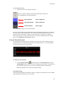
The Unit Display
In the Unit Display a single channel of candidate waveforms are grouped by unit, that is, each
individual plot displays all waveforms classified with a single sort code. Units are displayed from
left to right according to their numerical sort code. When present in the data set, unsorted
waveforms are assigned a sort code of "0" and will be displayed to the left of all other sort codes
with the label NS. If there are more units than can be displayed within the width of the tabbed
window, a scroll bar is displayed.
The PCSort control will display all possible sort codes based on the sorting algorithm or user
selections chosen.
The maximum number of sort codes (up to 5) that can be stored per channel to the hardware is
determined by the "maximum number of clusters" parameter in the PCSort macro. Based on these
limitations for data storage, the unit display uses color to distinguish between sort codes that can
be written to hardware (white) and those that cannot (red). In the example below, waveforms
assigned to sort code 5 in the display will be saved to the tank with a sort code of 31 (outlier).
White
Red
Reassigning Units using the Unit Display
The Unit display can be used to reassign units to different sort codes or combine two or more units
together into a single unit.
To reassign a sort code using the unit display:

Click and drag the desired unit to a new or existing unit and release the left mouse button.
Tool Buttons
The PCSort control features a set of buttons that allow you to work with all channels in the data
set.
Setup Properties
20
Open the Setup Properties dialog box.
The Tools
Auto Scale
Auto scale and normalize all plot displays. This does not auto
scale the feature space.
Base Scale
Return all channels to the base scale of 1.
Auto Track Threshold
Enables auto-tracking for all unlocked channels.
Manual Track Threshold Enables manual-tracking for all unlocked channels.
Clear All History
Clears event history for all channels.
Recalculate Feature Space Recalculate the feature space for all unlocked channels
depending on the training termination conditions (recalculates
the eigenvector to determine mapping for the feature space).
Accept Feature Space
Accepts the current feature space for all channels (uses the
currently calculated eigenvector for all channel principle
component mapping to the feature space).
Calculate Clusters
Automatically stops training, accepts the feature space, and
clusters the existing data for all unlocked channels.
Clears Clusters
Clears clusters for all unlocked channels and removes color
coding (also removes spheres).
Spheres
Displays the boundaries of spheres used to define cluster
shapes in the feature space.
Undo
Undo previous action (disabled if the active channel is
locked).
Redo
Redo an undone action (disabled if the active channel is
locked).
Lock
Locks clustering actions for all channels. Window resizing,
sphere toggle, channel selections, and acceptance of feature
space are still allowed. Locking any channel(s) automatically
accepts the feature space and ends training.
Unlock
Unlocks the controls mentioned above after they have been
locked for all channels.
Apply Sorts
Applies the software sorting information for all channels to the
processing chain running on the hardware.
21
SpikePac User’s Guide
Shortcut Menus
Right-clicking any snippet plot displays a shortcut menu that provides the following commands
for the active channel:
Clear History - Clears the display for the selected channel. Data saved to the Tank
remains unchanged.
Clear Clusters - Clears the currently selected channel’s clusters from the display; sort
codes saved to the Tank remain unchanged.
Auto Cluster - Stops training, accepts the feature space, and applies clusters to the data
for the selected channel.
Recalculate Space - Recalculate the selected channel’s feature space. Recalculating the
current channel re-evaluates the training termination conditions. For example, if the
default condition is: score > 95% OR Events > 1000 OR time > 300 secs, then the space
will be accepted immediately if any of these conditions are satisfied. See, page 11, for
more information.
Restart Space Calculation - Restarts the space calculation for the selected channel.
Note: only available while the training time is in progress.
Accept Space - Accept the selected channel’s feature space regardless of the training
status. Note: only available while the training time is in progress.
Lock/Unlock - Locks or unlocks the selected channel, preventing changes to clustering
for that channel.
Set Threshold Here (Manual Threshold mode only) – Sets the threshold for all
channels to the current mouse (pointer) position.
Auto/Manual Threshold – Toggles between Auto/Manual thresholding on the selected
channel.
Reset Scaling – Returns the active channel to its base scale of 1.
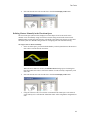
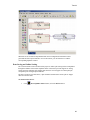
Working with the Selected Channel
Users can access the channel that is selected (active) within the PCSort control workspace by
using the <ID>_ChanSel parameter tag. This tag can be used within the RPvdsEx circuit, for
example, to pick off a single channel for additional processing. The example circuit below uses
the parameter tag to set the ChanSel parameter of an MCToSing component and send that channel
to additional processing components. The PCSort macro updates this parameter dynamically as the
active channel is changed (selected) through the PCSort control.
The tag’s unique name is generated using the PCSort macro’s three character Identity. In the
example below, the PCSort macro Identity is “Ne1” so the parameter tag is Ne1_ChanSel.
Channel Select Circuit Modification
22
The Tools
BoxSort - Time-Voltage Spike Sorting
BoxSort
Store (nChan=16)
SortCode
ID: Neu, Store: 'eNeu/pNeu'
The BoxSort macro is used to time stamp and store waveform events as data snippets and support
online spike sorting through the BoxSort control in OpenController. Candidate waveforms are
detected based on their deviation from the noise of the system. By default, the time stamp and
position of the waveform in the snippet is dependent on the time of the threshold crossing for the
signal. An alternative setting allows waveform time stamp and positioning to be determined by the
waveform’s highest peak, aligning snippets to their respective peaks. The macro can be configured
to output the sort code for each channel once sorting parameters have been loaded to the hardware
through OpenController.
This macro generates two data Stores: one for sorted snippet data, designated with the prefix e,
and one for the plot decimated data stream (a representation of the waveform using maximum and
minimum values and used to visualize spike activity), designated with the prefix p. The ID is
appended to the Store names and both are displayed in the macro’s parameter summary.
Settings for configuring the number of channels, threshold mode, and window width for each
snippet stored are defined in the macro properties dialog box. See the onboard macro help for
more information.
The corresponding BoxSort control set offers manual sorting using time-voltage box pairs to
classify potential units among candidate waveforms.
The BoxSort control set can be used to sort spikes online when the BoxSort macro is included in
the compiled circuit file. Spike detection is implemented by default and the user must enable spike
sorting.
23
SpikePac User’s Guide
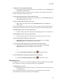
Tool Buttons
Threshold Display
Channel Select
Waveform Space
Multi-Channel
Display
Unit Display
The Control Set window includes:
Tool Buttons
provide access to tools and parameters.
Threshold Display
displays the plot decimated waveform of the currently selected channel
and allows threshold adjustments under manual thresholding mode.
Channel Select
used to select the active channel and display status information about
the channels.
Waveform Space
displays a time-voltage waveform representation of candidate spikes
for the active channel in a pile plot. In this plot, users can view and
manually classify waveforms by shape. Indicators in the bottom left
corner denote scaling and threshold tracking states.
Multi-Channel Display
displays each channel in a separate pile plot. The channel number is
shown in the bottom right corner of each sub-plot and waveforms are
highlighted as they are added to the plot. Clicking a sub-plot makes that
channel the active channel for the control. Indicators in the bottom left
corner denote scaling and threshold tracking states.
Unit Display
displays a single channel of candidate waveforms by unit—each plot
displays all waveforms classified with a single sort code. If there are
more units than can be displayed within the width of the window, a
scroll bar is displayed.
Simple Zoom
You can zoom any plot to see more or less detail. Zooming does not attempt to scale or fit the
waveform shape or data in the plot, allowing you to control the view without regard to the
limitations of the plot size.
24
The Tools
Note: changing the zoom level in the Multi-Channel Display alters the zoom level for all channels
in the Multi-Channel Display.
To change the zoom level of any plot:

Point to the center of the plot, press and hold down the Shift key, and drag the mouse up
or down.
To reset the view of any individual plot:

Hold down the Shift key and double-click the mouse within the plot.
Note: this method can be used to reset the feature space to its default position.
Display Scale
When the BoxSort control set is run, all channels begin at a base scale of 1. This type of scaling
clearly shows differences in magnitude across units but can make it more difficult to see
waveform shapes for some channels.
To make it easier to see waveform shapes for channels with lower magnitude, you may scale
individual channels manually or normalize all channels to fit to a similar scale. If you choose to
normalize the display, the BoxSort control set calculates the display scale for each channel
individually, attempting to fit around 80% of the signal’s vertical size in each plot.
When the display has been normalized, BoxSort displays either an up or down arrow in the bottom
left corner of the plot or subplot to indicate whether the display has been scaled up or down.
An Auto Scale feature can be used to refresh the scale of plots either with or without normalizing
the display.
To refresh the display without normalizing plots:
1.
Click the Auto Scale
button.
2.
Click No when asked if you want to normalize all window groups.
Note: this will not reset the feature space display.
To normalize all channels:
1.
Click the Auto Scale
button.
2.
Click Yes when asked if you want to normalize all window groups.
Note: an arrow will now be displayed on the bottom left corner (next to the threshold
mode indicator) which indicates positive or negative deviation from the base scale
setting.
To return all channels to their base scale:
1.
Click the Base Scale
2.
Click Yes.
button.
Note: resetting plots to base scale does not remove any Zoom applied to a plot.
25
SpikePac User’s Guide
To adjust the scale of a single channel:

Point to the desired channel in the Multi-Channel display, press and hold down the Ctrl
key, and drag the mouse up or down.
Note: while adjusting the display scale, the numeric value in the lower right corner of the
channel indicates the new scale value.
To return a single channel to its base scale:
1.
Right-click the desired channel.
2.
Select Reset Scaling from the menu.
The Setup Properties
Users can configure the thresholding control and enable or disable the use of bi-directional
thresholding by selecting positive or negative from the Default Search Polarity drop-down box.
To open the setup properties:

Click the Setup Properties
button.
Thresholding Parameter Group
Threshold Factor – Select a value to set base threshold for spike detection to a value
which is n * STD of the signal RMS. This setting is active only when automatic threshold
tracking is enabled.
Threshold Window Time Span – Type a numeric value to set the time span of the
threshold window in seconds. Note: the control must be restarted to alter the time span.
Default Search Polarity – Select a positive or negative polarity for the threshold value.
This setting is active only when automatic threshold tracking is enabled.
Default Peak Alignment – Sets the default alignment to Peak Align which aligns spikes
according to their peak values altering the time stamp and positioning of the snippet.
Track Time Const – Sets the time constant tau to 3, 5, or 10 seconds. Shorter tau values
respond more drastically to deviations in the signal RMS value. This setting is active only
when automatic threshold tracking is enabled.
Artifact Rejection Level (µV) – Type a numeric value to set the artifact rejection level
in micro Volts. Note: Artifact Rejection must be enabled in the macro setup properties in
RPvdsEx.
26
The Tools
Display Parameter Group
Clear History Counter – Enter a number to set a limit on the number of events
displayed prior to a display refresh. This does not delete historical data from the data
tank. It simply removes existing data displays and refreshes each plot. With the default
setting of 0, plots will display accumulated historical data.
Max Channels To Display – Enter a number to limit the amount of channels that will be
displayed in the Multi-Channel Display. The channel select bar will reorganize into one
or more columns based on the settings applied. The default value is 64.
Channel Column Count – Enter a number to set the number of columns for the MultiChannel Display. With the default setting of 0, the BoxSort control will automatically
select the number of columns to display.
Display Layout – Select either Standard or MultiChannel View modes of display. In
Standard display mode the Threshold and Unit displays extend the entire width of the
control set (see page 23 for an example of the Standard Display Mode). In MultiChannel
View mode, the right side of the control set is used only for the Multi-Channel Display,
extending vertically from top to bottom. This provides more room for multi-channel
display.
Selecting the Active Channel
The channel selector bar along the left side of the control set (shown below) determines which
channel is displayed in all other single channel plots within the set and highlights the active
channel in the Multi-channel plot.
To set a channel as active:

Click the selector box for the desired channel.
The active channel is displayed in all single channel plots within the set and is highlighted in the
multi-channel plot.
Channel status:
The color of the selector switch displays the status of each channel.
Currently Selected Channel (Active)
Color is light blue.
Non-selected Channel
Color is dark blue.
Locked Channel*
Color is gray.
*See Tool Buttons on page 34, for more information.
27
SpikePac User’s Guide
Using the Threshold Control
The threshold control (shown below) displays the plot decimated waveform for the selected
channel along with the threshold marker. The default value specified for the threshold factor is 6.5
x STD (standard deviations from the waveform’s RMS value).
Threshold Tracking
Threshold tracking adjusts the threshold in response to changes in each channel waveform’s RMS,
using a default time constant (tau) of five seconds.
Note: tracking is performed on the DSP and is enabled by default in the BoxSort macro.
Automatically tracking the threshold on many channels of data can tax the processor; see Saving
Cycle Usage below if you are recording many channels.
When threshold tracking is active the threshold bar will be locked preventing manual adjustments.
An ‘A’ indicator is placed in the bottom left corner of the Waveform Space and Multi-Channel
Display plots to denote if threshold tracking is currently active for a given channel. Otherwise, an
‘M’ indicator will be shown to denote that threshold tracking is disabled.
Threshold tracking is active
for the current channel.
Threshold tracking is
disabled for the current
channel, allowing for manual
threshold adjustments.
To enable threshold tracking for all channels:
Note: automatic threshold mode must be enabled in the BoxSort macro setup properties.
1.
28
Click the Auto Threshold
button.
The Tools
2.
Click Yes to enable threshold tracking for all channels.
To enable or disable threshold tracking for individual channels:

Right-click on the desired channel and select either Auto Threshold or Manual
Threshold.
To disable threshold tracking for all channels:
1.
Click the Manual Threshold
button.
2.
Click Yes to disable threshold tracking for all channels.
Setting the Threshold Manually
When the corresponding channel is set to manual threshold mode, the threshold bar may be
adjusted manually in the threshold control window by clicking and dragging the threshold bar
(shown below).
Note: hold the ctrl key and
double click on the Threshold
Display to toggle threshold
tracking on or off for the active
channel.
Manual adjustments to the threshold can also be made in the waveform space as shown below.
To change the threshold for a single channel:

Click and drag the threshold bar to the desired location in either the Waveform Space or
Threshold Control plots.
To apply the current threshold setting for all channels:
Note: this will only set the threshold for channels in which threshold tracking is disabled.
1.
Right-click the desired threshold location in the Threshold Display.
2.
Select Set Threshold Here from the menu.
3.
Click Yes to apply the threshold setting to all channels in manual threshold mode.
29
SpikePac User’s Guide
Saving Cycle Usage
Threshold tracking relies on circuit components contained within the BoxSort macro. This means
that the DSP is continuously tracking the threshold while it is performing other tasks such as
filtering and acquisition. This process is taxing on the device cycle usage rates and may diminish
the ability of BoxSort to process higher channel counts. Threshold tracking can be disabled in the
circuit through the BoxSort macro setup properties. When disabled, only manual threshold mode
is available (signified by the manual threshold button being grayed out). Manual threshold
methods must be used to obtain the threshold settings but this frees up cycle usage on the DSP
enabling more processing.
In addition to disabling threshold tracking, the BoxSort control alters the functionality of the
Automatic Threshold button. When the button is clicked, an instantaneous calculation of the data
is performed by the PC to determine a reasonable threshold setting for all channels.
To instantly calculate the threshold for all channels:
Note: automatic threshold mode must be disabled in the BoxSort macro setup properties.
1.
Click the Auto Threshold
button.
2.
Click Yes to calculate the instantaneous threshold for all channels.
To instantly calculate the threshold for a single channel:
Note: automatic threshold mode must be disabled in the PCSort macro setup properties.
1.
Right-click on the desired channel.
2.
Select Auto Threshold from the menu.
Artifact Rejection
Artifact rejection is configured through the control setup properties window using the Setup
Properties
button. Once enabled, events that fall outside of the specified value are ignored.
Box Sorting Using the Waveform Space
The BoxSort control set utilizes a pair of color-coded boxes (one solid and one dotted) to classify
each unit. A total of eight box pairs are available for sorting candidate waveforms. Box sorting
allows units to be assigned based on a set of requirements defined for each unit.
Box Sort Unit Requirements
1.
Candidate waveforms must enter the solid box only one time.
2.
Candidate waveforms must contain data points that pass through both boxes in the pair.
3.
One digitized point of the candidate waveform must exist in each box.
The waveform space (shown below) displays all spike waveforms for the active channel. Users
can identify potential units by using mouse based manipulation tools.
30
The Tools
To manually adjust the boxes:

Use standard click and drag techniques on any of the 8 points to adjust the boundaries of
the boxes.

Click and drag the edge of a box to move it to the desired position.
Note: the mouse icon will indicate whether the box will be adjusted or moved.
To add a box pair:

Hold Ctrl + double click to add a new box pair to the waveform space.
Sort codes are automatically assigned to the newly added box pair.
Note: the maximum number of units available for the hardware is defined within the BoxSort
macro setup properties.
To remove a box pair:

Drag either the solid or dotted box out of the plot and click Yes when asked to remove
hand mark.
If a waveform passes through more than one box pair:

Sort code priority is assigned based on the sort code number. This means that the lower
sort code will win in the event that a waveform passes through more than one box pair.
31
SpikePac User’s Guide
Applying Sorts to New Data
Sort codes are not saved to the data tank until sorts are applied by the user. You can re-sort or
make adjustments as needed to get the best results.
To begin saving sort codes for all channels to the data tank:

Click the Apply Sorts
button.
Sort codes are applied as new data is acquired. Once sorts have been applied, any changes in
sorting parameters in the display will be applied automatically.
Clearing the Event History
The event history of individual channels as well as all channels may be cleared at any time and
will remove any displayed waveforms on the Waveform Space, Unit Display, and Multi-Channel
Display plots for the desired channel(s).
To clear the event history:

Right-click a plot for the desired channel, click Clear History on the shortcut menu.
or

Click the Clear All History button
and select Yes when asked to confirm.
Note: clearing the event history will not affect waveforms that have already been stored to the
data tank.
Clearing Sort Codes
To clear Sort codes:

Right-click a plot for the desired channel, click Clear History on the shortcut menu, then
click Yes when prompted to confirm.
or

Click the Clear All Sorts button
and click Yes when asked to confirm.
Note: clearing sort codes will not affect sorted waveforms that have already been stored to the
data tank.
32
The Tools
The Unit Display
In the Unit Display a single channel of candidate waveforms are grouped by unit, that is, each
individual plot displays all waveforms classified with a single sort code. Units are displayed from
left to right according to their numerical sort code. When present in the data set, unsorted
waveforms are assigned a sort code of "0" and will be displayed to the left of all other sort codes
with the label NS. If there are more units than can be displayed within the width of the tabbed
window, a scroll bar is displayed.
The BoxSort control will display all possible sort codes based on the user selections chosen.
The maximum number of sort codes (up to 8) that can be stored per channel to hardware is
determined by the "Max Sorts" parameter in the BoxSort macro. Based on these limitations for
data storage, the unit display uses color to distinguish between sort codes that can be written to
hardware (white) and those that cannot (red). In the example below, waveforms assigned to sort
code 5 in the display will be saved to the tank with a sort code of 31 (outlier).
White
Red
Reassigning Units using the Unit Display
The Unit display can be used to reassign units to different sort codes. Unlike PCSort, units cannot
be combined.
To reassign a sort code using the unit display:

Click and drag the desired unit to a new unit and release the left mouse button.
33
SpikePac User’s Guide
Tool Buttons
The BoxSort control features a set of buttons that allow you to work with all channels in the data
set.
Setup Properties
Open the Setup Properties dialog box.
Auto Scale
Auto scale and normalize all plot displays.
Base Scale
Return all channels to the base scale of 1.
Auto Track Threshold
Enables auto-tracking for all unlocked channels.
Manual Track Threshold Enables manual-tracking for all unlocked channels.
34
Clear All History
Clears event history for all channels.
Clear All Sorts
Clears all sort codes for all unlocked channels.
Undo
Undo previous action (disabled if the active channel is
locked).
Redo
Redo an undone action (disabled if the active channel is
locked).
Lock
Locks box sorting actions for all channels. Window resizing,
and channel selections are still allowed. Locking any
channel(s) automatically accepts the feature space and ends
training.
Unlock
Unlocks the controls mentioned above after they have been
locked for all channels.
Apply Sorts
Applies the software sorting information to the processing
chain running on the hardware.
The Tools
Shortcut Menus
Right-clicking any snippet plot displays a shortcut menu that provides the following commands:
Clear History – Select to clear all traces from the selected channel display, data saved to
the Tank remains unchanged. Any existing time-voltage bars will remain.
Clear Sorts – Select to clear any sorts for the currently selected channel. This removes
sort colors from the display; sort codes saved to the Tank remain unchanged.
Lock or Unlock the current channel – Select to toggle the locked or unlocked state of
the selected channel.
Set Threshold Here (Manual Threshold mode only) – Sets the threshold for all
channels to the current mouse (pointer) position.
Auto/Manual Threshold – Toggles between Auto/Manual thresholding on the selected
channel.
Reset Scaling – Returns the active channel to the base scale of 1.
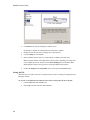
Working with the Selected Channel
Users can access the channel that is selected (active) within the PCSort control workspace by
using the <ID>_ChanSel parameter tag. This tag can be used within the RPvdsEx circuit, for
example, to pick off a single channel for additional processing. The example circuit below uses
the parameter tag to set the ChanSel parameter of an MCToSing component and send that channel
to additional processing components. The BoxSort macro updates this parameter dynamically as
the active channel is changed (selected) through the BoxSort control.
The tag’s unique name is generated using the BoxSort macro’s three character Identity. In the
example below, the BoxSort macro Identity is “Ne1” so the parameter tag is Ne1_ChanSel.
Channel Select Circuit Modification
35
SpikePac User’s Guide
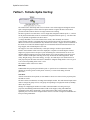
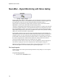
TetSort - Tetrode Spike Sorting
The TetSort macro timestamps and stores waveform events as data snippets and supports online
spike sorting through the TetSort control in OpenController. Together the macro and control
provide a flexible software interface for single-unit tetrode recording.
The macro generates two data Stores: one for snippet data, designated with the prefix ‘e’, and one
for the plot decimated data stream for visualization, designated with the prefix ‘p’. The macro ID
(‘Tet’ by default) is appended to the Store names.
A voltage threshold is set for each channel of the tetrode, either manually in TetSort’s
OpenController interface or automatically based on the deviation of the waveform from its RMS.
When a waveform crosses threshold on any channel in the tetrode, a snippet on all four channels in
the tetrode is recorded. The channel snippets are concatenated and stored in the data tank as one
large snippet, with a timestamp and a sort code.
The snippet’s sort code is determined by visual spike sorting in TetSort’s OpenController
interface. Each channel within a tetrode is displayed in a separate waveform subplot. Channel
snippets are projected onto a 2D space by first calculating user-selected metrics for one or two
channels and then mapping one metric against another. Up to four 2D feature projections can be
used to visualize tetrode spike clustering. Users may select from the following metrics: Peak,
Valley, Height, Energy, Non-Linear Energy, Average, Area and Slope. User-defined circles in
each projection plot determine each cluster's boundaries. Snippets falling inside a circle are given
a sort code corresponding to that circle’s color.
The TetSort control works in two modes:
Hunt Mode
In Hunt Mode the projection plots default to peak vs. peak for all six combinations of tetrode
channels to provide a general overall picture of activity. Use this mode during electrode
placement.
Sort Mode
After the electrode has been placed, use Sort Mode to choose new metrics for the projection plots
and add sort circles.
The macro allows simultaneous recordings from multiple tetrodes. The multi-channel input stream
must be arranged in groups of four; each group corresponding to one physical tetrode (a SiteMap
macro may be used).
Settings for configuring the number of tetrodes, maximum number of sorting circles per
projection, thresholding method and window width of the snippets, along with additional
explanation of the macro functionality, can be found in the TetSort macro properties dialog.
Optionally, the sort codes can be output from the macro as a stream of integers for additional realtime processing in RPvdsEx.
36
The Tools
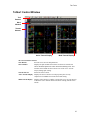
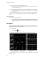
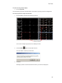
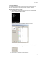
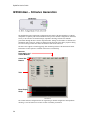
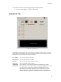
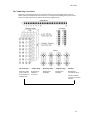
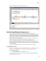
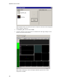
TetSort Control Window
Tool
Buttons
Wave
Window
Tetrode
Selector
Active Tetrode Display
Multi-Tetrode Display
The Control Window includes:
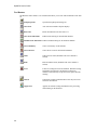
Tool Buttons
Provides access to tools and parameters.
Wave Window
Displays the plot decimated waveforms for the active tetrode and
allows threshold adjustments under manual thresholding mode. This
window can be hidden to allow a better view of the Active Tetrode
Display during spike sorting.
Tetrode Selector
Selects the active tetrode.
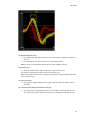
Active Tetrode Display Displays the active tetrode in several projection plots for easy
comparison of candidate waveforms and visual sorting.
Multi-Tetrode Display
Displays each tetrode in a smaller version of the Active Tetrode Display
to allow the user to monitor all tetrodes while working with the active
tetrode.
37
SpikePac User’s Guide
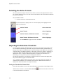
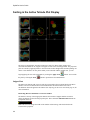
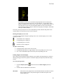
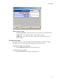
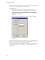
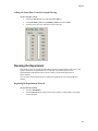
Selecting the Active Tetrode
The Tetrode Selector along the left side of the control set (shown to the right) determines which
set of tetrode channels is active. The color of the tetrode indicator in the Tetrode Selector indicates
the status of each tetrode.
To set a tetrode as active:

Click the selector box for the desired tetrode.
The selected tetrode is displayed in Active Tetrode Display and is highlighted in the
Multi-Tetrode Display.
Inactive Tetrode
Color is dark blue
Active Tetrode
Color is light blue.
Inactive Tetrode, All Channels Locked*
Color is gray
Active Tetrode, All Channels Locked*
Color is light gray.
*See Tool Buttons on page 20 for more information.
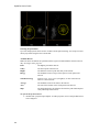
Adjusting the Detection Threshold
To begin acquiring snippets, thresholds must be set for at least one channel of the tetrode. There
are two methods of determining a threshold: setting the threshold manually (Manual Mode) or
letting TetSort compute a threshold based on a specified multiple of the RMS level of the signal
(Automatic Mode). This RMS calculation is continuously performed to adjust for fluctuations in
system noise. Note: Automatic mode requires extra processing on the DSP and is disabled by
default in the macro. It must be enabled in the macro if you want to use this feature; see
Minimizing Cycle Usage below if you are recording many channels.
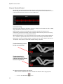
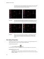
The white threshold bars for each channel are displayed in the wave window and snippet plots.
They will automatically appear in Automatic Mode.
An ‘A’ indicator is displayed in the bottom left corner of the snippet plots if the channel is in
Automatic mode. Otherwise, an ‘M’ indicator will be shown to denote that the channel is in
Manual mode and the threshold can be adjusted manually.
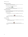
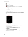
Setting the Threshold in Manual Mode
If the white threshold bars are not visible in Manual Mode, and Automatic Thresholding has been
disabled in the circuit macro, click the Auto Threshold
a reasonable threshold for all channels.
38
button and Controller will calculate
The Tools
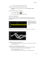
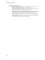
To change the threshold for a single channel:

In Manual threshold mode, click and drag the threshold bar to the desired location in
either the scrolling waveform or pile plots.
To apply a threshold using point and click:
Note: This will only set the threshold for channels in Manual mode.
1.
Right-click the desired threshold location in the waveform display and click Set
Threshold Here in the shortcut menu.
2.
Click Yes to apply the threshold setting to all channels in manual threshold mode.
Automatic Threshold Tracking (Automatic Mode)
Threshold tracking adjusts the threshold in response to changes in each channel’s waveform RMS
using a default time constant (tau) of five seconds. The default value specified for the threshold
factor is 6.5 x STD (standard deviations from the waveform’s RMS value). The time constant and
threshold factor can be modified in the control’s setup properties.
To change the threshold factor or time constant:

Click the Setup Properties
button and select a new Threshold Factor and Track
Time Const from the Thresholding parameter group. See page52 for more threshold
parameter setting options.
When threshold tracking is active the threshold bar will be locked, preventing manual adjustments.
To enable threshold tracking for all channels:
1.
Click the Auto Threshold
button.
2.
Click Yes to enable threshold tracking for all channels.
To disable threshold tracking for all channels:
1.
Click the Manual Threshold
button.
2.
Click Yes to disable threshold tracking for all channels.
To disable threshold tracking for individual channels:

Right-click on the snippet plot and select Manual Threshold.
Working with the Plots
Zoom and Pan
Zoom and Pan are used to see more or less detail or to focus on a specific area of the plot.
To change the zoom level of any plot:

Point to the center of the plot, press and hold down the Shift key, and drag the mouse up
or down.
To pan in snippet plots:

Hold down the Alt key, click and drag to move the snippets vertically.
39
SpikePac User’s Guide
To pan in projection plots:

Click and drag to move the view.
Scale
In addition to an overall scale factor, each channel has its own individual scale factor (base scale)
for normalizing the display of all channels in the Wave Window and Snippet Plots. All channels
begin with a base scale of 1. Using the auto scale feature, you can refresh the scale of plots either
with or without normalizing the display.
Note: Changing any display scale factor does not alter the data being stored.
If you choose to normalize the display, TetSort calculates the display scale for the each channel,
attempting to fit around 80% of the signal’s vertical size in each waveform plot. When the display
has been normalized, TetSort displays either an up or down arrow in the bottom left corner of the
snippet plots to indicate whether the display has been scaled up or down.
TetSort stores two sets of scale factors, one set for Sort mode and another for Hunt mode. Each set
(Sort or Hunt) of scaling information includes a scale factor for the tetrode and any individual
scale factors set for individual plots. This allows you to switch between modes without rescaling
or losing scaling information.
To refresh the display without normalizing plots:
1.
Click the Auto Scale
button.
2.
Click No when asked if you want to normalize all window groups.
To normalize all channels:
1.
Click the Auto Scale
button.
2.
Click Yes when asked if you want to normalize all window groups.
To reset all channel and projections base scales:

Click the Reset Base Scale
button.
To return all channels of a single tetrode to their base scale:

Right-click in the Wave Window and select Reset Scaling – Tetrode.
To return a single channel to its base scale:

Right-click in the corresponding Snippet Plot and select Reset Scaling.
Scaling the Projection Plots
In addition to being scaled when all plots/channels are scaled, the projection plots can be scaled
for each tetrode or as individual plots. When a projection plot has been scaled, an arrow will
appear in the bottom left corner to indicate the direction to the origin point of the plot.
To adjust the scale of all projection plots for a tetrode:

40
Right-click any projection plot in the Active Tetrode Display, point to Auto Scale, and
click Tetrode on the shortcut menu.
The Tools
To adjust the scale of a single projection plot:

Right-click the desired projection in the Active Tetrode Display, point to Auto Scale, and
click Plot on the shortcut menu.
The projection plots also have a base scale which is computed as a reasonable estimate based on
the metric combinations and typical data sets.
To return all projection plots for a tetrode to the base scale:

Right-click any projection in the Active Tetrode Display, point to Reset Base Scale, and
click Tetrode on the shortcut menu.
To return a single projection plot to its base scale:

Right-click the desired projection, point to Reset Base Scale, and click Plot on the
shortcut menu.
Because the 2D clusters don’t always fit into nice circles for sorting, the projection plot axes can
be independently scaled in order to skew the data set so that it does fit into a circular boundary.
To independently scale the x-axis of a projection plot:

Hold down Ctrl + Alt, click the left mouse button and drag the cursor to the right or left.
To independently scale the y-axis of a projection plot:

Hold down Ctrl + Alt, click the left mouse button and drag the cursor up or down.
To reset the independent scaling for a projection plot:

Right-click the desired projection in the Active Tetrode display, point to Reset
Independent Scale, and click Plot on the shortcut menu.
To reset the independent scaling for all projection plots in the current tetrode:

Right-click the desired projection in the Active Tetrode display, point to Reset
Independent Scale, and click Tetrode on the shortcut menu.
or

Click the Reset 2D Plot Independent Scaling
button and select No.
To reset the independent scaling for all projection plots in all tetrodes:

Click the Reset 2D Plot Independent Scaling
button and select Yes.
Highlighting Traces
By default, the most recent trace acquired is highlighted in all plots throughout the tetrode display
area. Alternatively, a group of traces that are of interest can be highlighted.
To highlight a group of traces:

Hold down the a key and drag the pointer across the desired traces in any pile plot in the
tetrode display area.
This can be repeated to add to more selected traces. The selected pile plot traces and their
corresponding dots in the projection plot(s) will be highlighted.
41
SpikePac User’s Guide
To remove a group of traces from the highlighted selection:

Press and hold down the s key and drag the pointer across the desired traces in any pile
plot in the tetrode display area.
To return to the default highlight mode (most recent trace highlighted as plots are updated):

Press and hold down the s key and drag the pointer across all traces in any pile plot in the
tetrode display area.
To the right of the projection plot, and below the column of filtering icons, the
highlighting
icon can be clicked to clear highlighting from the projection plot and pile plots of the active
tetrode.
Audio Monitoring
To select a channel for audio monitoring:

Press and hold down the c key and click the corresponding pile plot in the tetrode display
area. A speaker icon will appear in the bottom right of the pile plot. This sends the
currently selected channel to a NeuroMon macro with the same ID as this TetSort macro,
e.g. ‘Tet’.
Hunt Mode
Hunt mode is designed for use during electrode placement. In this mode, the feature projections
show peak vs peak for all electrode combinations to provide a general overall picture of activity.
By default, the TetSort controller is in Sort Mode.
To turn on Hunt mode:

Click the Hunt
button.
All sorting features are disabled in this mode, but scaling and other features are available.
The number of events that are shown in the snippet plots and projection plots can be configured in
the Setup Properties.
42
The Tools
To clear all events from the display:

Press the Spacebar.
You can transfer projections from Hunt mode to Sort mode to speed up projection configuration.
To select projections to transfer to Sort mode:
1.
Press the Ctrl key and click the desired projection(s).
You can select multiple projections across multiple tetrodes.
2.
Click the Hunt
button to turn Hunt mode off.
You’ll be asked to confirm your selections.
3.
Click Yes.
The display returns to Sort mode and the selections you selected are displayed.
43
SpikePac User’s Guide
Sorting in the Active Tetrode Plot Display
The Active Tetrode display provides an interactive space for online cluster cutting. Once
reasonable thresholds are set, snippets will appear in each of the four Snippet Plots. The projection
plots are created by applying metrics to the waveforms in these Snippet Plots and then plotting one
metric versus another in an X-Y plane. When you are satisfied with the defined sorts, you can
begin applying the sort codes in hardware by clicking the Apply Sorts
the plots by clicking the Lock
button. You can lock
button to protect them from modification.
Snippet Plots
The label in the bottom right corner of each plot corresponds to the waveform labels in the Wave
Window. An arrow in the bottom left corner indicates the direction from the base scale if
normalization has been applied to the channel. See Adjusting the Detection Threshold, page 38, for
more information.
Restricting Metric Calculations to a Narrow Window
The marker at the top of the snippet plot indicates the window of snippet data that is used for
metric calculations for the selected projection plot. This is called the Min-Max Interval and can
be adjusted on the fly.
Note: This does not change the width of the window in data storage, which is defined in the
TetSort macro properties.
44
The Tools
To adjust the Min-Max Interval:

Drag the yellow (Min) and/or red (Max) indicators to the desired position.
To reset the Min-Max Interval to the entire window width for one channel in the current
projection plot:

Right-click the snippet plot and click Reset Min-Max Interval on the shortcut menu.
To reset the Min-Max Interval to the entire window width for all channels for all projections of
the current tetrode:

Click the Reset Snippet Plot Max Min Intervals
select No.
button on the shortcut menu and
To reset the Min-Max Interval to the entire window width for all channels for all projections for
all tetrodes:

Click the Reset Snippet Plot Max Min Intervals
select Yes.
button on the shortcut menu and
Projection Plots
The main area of the active tetrode display is divided into four 2D projection plots for dynamic
visual spike sorting. Each snippet appears as a single dot in 2D space of one metric plotted versus
another. By default, the top left plot will display the peak of the first channel against the peak of
the second channel.
User-defined circles are drawn around dots to assign sort codes to their associated snippets.
Snippets falling inside a circle are given a sort code corresponding to that circle’s color. The color
of the dot representing that snippet will change to the color of the circle. More than one circle of
the same color can be defined in each projection. A snippet falling in any of those same-colored
circles will be classified with that sort code.
Because snippets can fall into more than one circle, the actual sort code stored in the data tank is a
mask of all sort codes that the candidate snippet fell inside. For example, if a snippet falls into a
yellow (sort code 1) and green (sort code 6) circle, then the snippet mask will be 33 (0b100001 =
33). In this case, the color of the dot used to define the snippet in the projection plot is randomly
chosen from the sort codes in the mask. A snippet that doesn’t fall inside any circles is considered
unsorted and has sort code 0.
If there are circles of the same color on more than one projection, a candidate snippet has to fall
inside that type of circle in all projections to be given that color’s sort code. The total number of
circles that can be defined in any one projection plot is set in the macro properties (default is 12).
45
SpikePac User’s Guide
Choosing Projection Plots
Up to four 2D projections can be used to visualize tetrode spike clustering. You can preview and
choose projections using the active tetrode data.
Available Metrics
Note: All metric calculations are performed on the segment of data within the min-max interval
only. See Snippet Plots, page 44.
Peak
The highest point in the interval.
Valley
The lowest point in the interval.
Height
The difference between peak and valley in the interval.
Energy
The arithmetic mean (average) of the squares of each point in the
interval.
Non-linear Energy
sum(w(t)*w(t) - w(t-1)*w(t+1))/length(w), for all t in the interval,
where w is the waveform.
Average
The arithmetic mean of all values in the interval.
Area
The sum of the absolute values of all points in the interval.
Slope
The height divided by the difference between the peak timestamp and
valley timestamp in the interval.
To open the Projection Selector:

46
Double-click a projection plot subplot. To add a projection, select a sub-plot that has not
been configured.
The Tools
In the Projection Selector you can choose from a variety of metrics combinations for visualization.
Each new projection can help to further refine a sort or identify new sorts. All possible
combinations of metrics between channels are displayed. The letters in the lower-right corner of
each plot indicate the x-axis and y-axis channels for that plot. Metric combinations that are already
in use in other projection plots for this tetrode will have a solid border around them.
Slide Switches on the left and bottom edges of the selector can be used to select Peak, Valley,
Height, Energy, Non-Linear Energy, Average, Area, or Slope for the X and Y axes.
The Sort Selection Display can be used to toggle the display of individual or all sort codes and
functions like the sort filter in the Active Tetrode Display. See Filtering the Display by Sort Code,
page 51, for more information.
The Toolbar provides access to tools that may be used while working in the Projection Selector
window.
Shows all data as unsorted events
Switch to corresponding projection (only available in plots that are already configured)
Go to selected (cluster projection preview within the selector)
47
SpikePac User’s Guide
Auto scale projections
Resets base scale for projections
Reset independent plot scaling removes any x-axis or y-axis skew in all available
projections.
To select a projection in the Projection Selector:
1.
Click the desired projection preview.
2.
Click Select.
Viewing Data in the Projection Plot
The feature projection plots can be zoomed, panned or scaled individually or by tetrode. See
Working with the Plots page 39 for more information. When the projection plot contains data that
is not in view, small carrots are positioned on the edge of the plot to indicate the direction of the
data.
When the origin point of the feature projections plot is not in view, an arrow is displayed in the
bottom left corner of the plot to show the direction of the origin point.
To center the origin in the plot:

Right-click the plot and click Center Origin on the shortcut menu.
To clear the history:

Right-click the plot and click Clear Tetrode History.
The number of points visible in the projection plot is controlled by the Projection Plot Display
History Depth setting in the properties dialog.
48
The Tools
Using Circles to Define Sorts
User-defined circles are drawn in each projection plot to determine a cluster's boundaries and
shape. Sort codes are applied to snippets using the boundary calculated for each cluster.
To create a sort circle and assign a sort code:
1.
Point to the desired projection in the Active Tetrode display, press and hold down the
Ctrl key, click and drag the mouse up or down.
When the mouse key is released the Assign New Sort code dialog opens.
The Sort Code list displays the available sort codes and associated colors (Cluster) and
the number of events (nEV) in each cluster. Sort-0 is unsorted events.
2.
Click the sort button in the Next Empty Code box or click the desired code in the list.
3.
Repeat this process until all likely sorts have been defined.
49
SpikePac User’s Guide
Arbitrary Shapes
Sort circles can also be generated by drawing an arbitrary shape around traces in a projection plot.
TetSort will then attempt to draw circles that will efficiently represent the selected traces. Users
can control how TetSort creates the circles using the Arbitrary Shape Uniform Distribution
check box in the Sort Display parameter group of the setup properties, see page 53 for more
information.
To create sorts by drawing an arbitrary shape:
1.
Press and hold the ALT key then hold down the mouse button and drag within the
plot to create an arbitrary shape.
2.
When the mouse key is released the Assign New Sort code dialog is opened.
3.
Click the sort button in the Next Empty Code box or click the desired code in the
list.
TetSort automatically creates circles to define the shape.
50
The Tools
The number of circles it uses to define the shape depends on how accurately the
shape can be approximated with circles. The Sort Display > Cluster Radius xSTD
property determines how close the circle centers can be. An arbitrary shape close to a
circle will only use one circle. The maximum number of circles it will use when
approximating an arbitrary shape is defined in the property Sort Display > Maximum
Circles per Arbitrary Shape.
If necessary, the projection plot axes can be independently scaled so that the data points fit into
circular clusters. See Scaling the Projection Plots, page 40.
Filtering the Display by Sort Code
A column of colored squares along the right edge of the Active Tetrode display serves to filter
events by sort code.
All available sorts are displayed
Corresponding sort is displayed
Corresponding sort is not used
Unsorted events are displayed
The filters can be used by:

Clicking the black square to show all sort codes.

Clicking individual squares to toggle display of the corresponding sort code on or off.

Ctrl + click an individual square to show only the corresponding sort code.
Pruning Snippets from the Display
Three options to Prune Snippets from the display are provided in the Setup Properties. Similar to
filtering, pruning provides more options to control the display and temporarily hide data during
sorting.
To use the pruning options:
1.
Click the Setup Properties
group.
2.
Click the desired combination of check boxes.
Threshold
button and select the Prune Snippets parameter
when selected, only snippets that crossed the threshold for the channel on which
they occurred are shown. The pruned snippets are hidden in all plots in the
tetrode display area.
51
SpikePac User’s Guide
The window on the left shows the display with no pruning selected. On the right,
only traces that meet the threshold for the channel in which they occurred are
shown. Only the data of interest for sorting is shown.
Sort Code
when selected, only show snippets if the projection plot containing a sort circle
uses a metric from that channel. Hides snippets on channels not used in the
projection plot metrics from the pile plots. See before and after images below.
Exclusive
Shows traces only in the pile plot in which the corresponding sort code first
appears. Note: this will always be the pile plot for the first channel of the
tetrode, unless used in conjunction with the threshold or sort code pruning
options.
The Setup Properties
TetSort control’s properties are used to configure the workspace layout, thresholding parameters,
history depths and other settings for both Sort Mode and Hunt Mode.
To open the setup properties:

Click the Setup Properties
button.
The Setup Properties window includes four parameter groups available from a drop down list.
Thresholding Parameter Group
Threshold Factor – Select a value to set base threshold for spike detection to a value
which is x * STD of the signal RMS. This setting is active only when automatic threshold
tracking is enabled.
52
The Tools
Threshold Window Time Span – Type a numeric value to set the time span of the
threshold window in seconds. Note: the control must be restarted to alter the time span.
Default Search Polarity – Select a positive or negative polarity for the threshold value.
This setting is active only when automatic threshold tracking is enabled.
Default Peak Alignment – Peak Align aligns spikes according to their peak values,
altering the time stamp and positioning of the snippet.
Track Time Const – Sets the time constant tau to 3, 5, or 10 seconds. Shorter tau values
respond more quickly to deviations in the signal RMS value. This setting is active only
when automatic threshold tracking is enabled.
Artifact Rejection Level (µV) – Type a numeric value to set the artifact rejection level
in micro Volts. Note: Artifact Rejection must be enabled in the macro setup properties in
RPvdsEx.
Common Display Parameter Group
Tetrode Column Count – Enter a number to set the number of columns for the MultiTetrode Display.
Max Tetrodes To Display: how many tetrodes to show in Multi-Tetrode Display.
Channel Index Type (A...D, 1...4, Absolute): how the channels inside each tetrode
should be labeled. A, B, C, D... 1, 2, 3, 4... Absolute means the actual preamp channel is
used.
Display Layout (Standard, MultiChannel View): Multichannel shortens the Wave
Window and increases the Multi-Tetrode Display.
Sort Display Parameter Group
Snippet Plot Display History Depth: how many snippets to show in Snippet Plots in
Sort Mode. 0 (default) means the 1024 most recent are shown.
Projection Plot Display History Depth: how many events to show in Projection Plots in
Sort Mode. 0 (default) means the 1024 most recent are shown.
Clear on full: when checked, the Snippet Plots and Projection Plots clear when the event
count reaches the display history depth specified above for the respective plots in Sort
Mode. Otherwise, a circular buffer is used to display the most recent events.
Show Wave Window: when unchecked, the Wave Window is not shown in Sort Mode.
Show Snippet Plots: when unchecked, the Snippet Plots in the Multi-Tetrode Display
are not shown in Sort Mode.
Show Projection Plots: when unchecked, the projection plots in the Multi-Tetrode
Display are not shown.
Cluster Radius xSTD: determines how close the circle centers can be when
approximating arbitrary shapes.
Maximum Circles per Arbitrary Shape: maximum number of circles to draw when
approximating an arbitrary shape.
Arbitrary Shape Uniform Distribution: when unchecked, the empty spaces within the
arbitrary shape are not considered significant and TetSort creates circles that tightly
conform to the selected points in the projection. When checked, a bounding box is first
created to contain the area within the arbitrary shape, and then circles are created to cover
all areas within the bounding box. Both options use the minimum number of circles
possible and no more than the user specified maximum.
53
SpikePac User’s Guide
Hunt Display Parameter Group
Snippet Plot Display History Depth: how many snippets to show in Snippet Plots in
Hunt Mode. 0 (default) means the 1024 most recent are shown.
Projection Plot Display History Depth: how many events to show in Projection Plots in
Hunt Mode. 0 (default) means the 1024 most recent are shown.
Clear on full: When checked, the Snippet Plots and Projection Plots clear when the event
count reaches the display history depth specified above for the respective plots in Hunt
Mode. Otherwise, a circular buffer is used to display the most recent events.
Show Wave Window: when unchecked, the Wave Window is not shown in Hunt Mode.
Show Snippet Plots: when unchecked, the Snippet Plots in the Active Tetrode Display
and the Multi-Tetrode Display are not shown in Hunt Mode.
54
The Tools
Tool Buttons
The control features a set of buttons that allow you to work with all channels in the data set.
Properties
Open the Setup Properties dialog box.
Auto Scale
Auto scale and normalize all plot displays.
Reset Base Scale
Return all displays to the base scale of 1.
Auto Threshold
Enables auto-tracking for all unlocked displays.
Manual Threshold
Enables manual-tracking for all unlocked
tetrodes.
Clear All Data
Clears event history for all tetrodes.
Clear All Sort Circles
Clear all sort circles for current tetrode or for all
tetrodes.
Reset Snippet Plot Min-Max Intervals Reset min-max intervals to endpoints of
waveform for current tetrode or for all tetrodes.
Reset 2D Plot Independent Scaling
Resets independent x-axis and y-axis scaling
factors.
Undo
Undo previous action (disabled if the active
tetrode is locked).
Redo
Redo an undone action (disabled if the active
tetrode is locked).
Lock All
Locks all tetrodes. Window resizing and tetrode
selections are still allowed.
Unlock All
Unlocks the controls mentioned above after they
have been locked for all tetrodes.
Hunt Mode
Switches to Hunt mode.
Hardware Sort
Applies the software sorting information for all
channels to the processing chain running on the
hardware.
55
SpikePac User’s Guide
Keyboard Shortcuts
Keyboard combos:
Click + Drag
Pan Projection Plot.
Shift + Click and Drag
Projection Plot: Zoom in and out.
Snippet Plot: Y-axis zoom.
Ctrl + Alt + Click and Drag
Skew the Projection Plots up down or left right.
Alt + Click and Drag
Snippet Plot: Pan.
Projection Plot: Draw arbitrary shape.
Keyboard Projection Plot hotkeys:
~
Show all sort codes.
1-9
Toggle sort code show/hide.
Ctrl + [1-9]
Show only the selected sort code.
Minimizing Cycle Usage
There are several features of TetSort that rely on additional circuit components within the macro.
These additional components raise the device cycle usage rates and may diminish the ability to
process higher channel counts.
Automatic threshold tracking relies on circuit components that continuously compute the threshold
while the DSP is performing other tasks such as filtering and acquisition. When automatic
thresholding is disabled, only manual threshold mode is available (signified by the manual
threshold button being grayed out). The TetSort control also alters the functionality of the
Automatic Threshold button. When the button is clicked, an instantaneous calculation of the data
is performed by the PC to determine a reasonable threshold setting for all channels.
To instantly calculate the threshold for all channels:
Note: Automatic threshold mode must be disabled in the macro setup properties.
1.
Click the Auto Threshold
button.
2.
Click Yes to calculate the instantaneous threshold for all channels.
To instantly calculate the threshold for a single channel:
Note: Automatic threshold mode must be disabled in the macro setup properties.
1.
Right-click on the desired channel’s Snippet Plot.
2.
Select Auto Threshold from the menu.
Artifact rejection also requires additional circuit components. Consider disabling artifact rejection
as a means of reducing cycle usage when using high channel counts.
The sort codes can be output from the circuit macro as a multi-channel stream of integers for
further processing. If this functionality is not being used, be sure to disable Sort Code Output in
the circuit macro.
56
The Tools
Working with the Selected Channel
Users can access the channel that is currently selected for audio monitoring within the TetSort
control workspace by using the <ID>_ChanSel parameter tag. This tag can be used within the
RPvdsEx circuit, for example, to pick off a single channel for additional processing. The example
circuit below uses the parameter tag to set the ChanSel parameter of an MCToSing component and
send that channel to additional processing components. The TetSort macro updates this parameter
dynamically as the monitored channel is changed (by holding c and clicking on any pile plot)
through the TetSort control.
The tag’s unique name is generated using the TetSort macro’s three character Identity. In the
example below, the TetSort macro Identity is “Te1” so the parameter tag is Te1_ChanSel.
Channel Select Circuit Modification
57
SpikePac User’s Guide
IZ2StimGen – Stimulus Generation
The IZ2StimGen macro implements configuration and control of the IZ2 Stimulator. It supports
monophasic or biphasic pulse train stimulation with up to four stimulus configurations. It features
an easy-to-use interface for stimulus design, impedance checking, and real-time stimulus
presentation through the IZ2 Control in OpenController. Settings for the number of channels and
stimulation mode (current or voltage) are defined on the Setup tab of the macro properties dialog
box. These settings control unit values and channel count for the control set.
The macro also supports external triggering, data monitoring and use of the IZ2H model. More
information on these options is available in the macro’s internal help.
Stimulus
Presentation and
Control Buttons
Control Set
Buttons
Tabs
Burst Display
Graph
The Control
The control includes configuration tabs for signal design, channel configuration and impedance
checking, as well as buttons for real-time control of stimulus presentation.
58
The Tools
The Control Set window includes:
Buttons
Set options and control stimulus presentation.
Voice Tabs
Design up to four unique pulse and burst parameter sets.
Train Tab
Design train parameters.
Config Tab
Configure each electrode channel mode.
Impedance Tab
Check impedance of each electrode bank.
The Buttons
The IZ2 Control features two sets of buttons: one for basic control set options and a second for
stimulus presentation and control.
Control Set
Lock
Lock the Voice Tabs options.
Unlock
Unlock the Voice Tabs options.
Undo
Undo last action in Voice Tab.
Redo
Redo last undone action in Voice Tabs.
Open
All channels are left Open (disconnected from the stimulator circuit)
when not stimulating. When a stimulation button is pressed, all
channels are set to the desired mode, 200ms later the trigger is sent.
200ms after the BUSY indicator goes dark all channels are opened
again until the next stimulation button is pressed.
Note: this mode is not available in External Trigger mode.
Stimulus Presentation and Control
Pulse
Send one pulse.
Burst
Send one burst.
Train
Send one train.
Continuous Run pulse trains continuously.
Stop
End stimulus presentation prematurely.
Busy
Busy LED is on when a stimulus is presented or impedance checking is
active. Changes to the stimulus configuration can only be applied when
Busy LED is not lit.
59
SpikePac User’s Guide
Note: When a signal longer than 0.5 seconds is presented, all buttons, except Stop, are disabled
during stimulus presentation to prevent changes. The Voice Tabs parameters are also locked.
These buttons will all be disabled if Workbench is in Idle mode, or if no channels are set to
stimulate. The Train and Continuous buttons will be disabled in External Trigger mode.
Burst Display Graph
This graph displays the burst waveform for reference. Users can move or scale waveforms for
better viewing. Note that this graph requires video drivers with OpenGL support. If the
appropriate video drivers are not installed, a blank graph is displayed.
To move the waveform in the diagram window:

Click and drag from side to side.
To adjust the x-axis scale of the plot:

Press and hold the Ctrl key and use the mouse wheel to zoom in and out on the x-axis
scale.
To adjust the y-axis scale of the plot:

Use the mouse wheel to zoom in and out on the y-axis scale.
To reset the axis or auto scale the plot:

Right-click the diagram and click the desired command on the shortcut menu.
The Shortcut Menu
Reset Scale X
Reset the X-axis scale to fit the entire waveform.
Reset Scale Y
Reset the Y-axis scale to the maximum values.
Auto Scale
Change the Y-axis scale to fit the waveform in 80% of the window.
Note: The Burst display is not shown in the Impedance tab.
Designing the Stimulus
The IZ2 Control interface breaks down the stimulus design process into hierarchical parts. Signal
design begins with the most basic component of the signal—the pulse. Once the pulse is defined,
the burst and then the train can be defined with each step referencing the one before.
The Signal Design Process
60
The Tools
The IZ2 Control supports up to four unique stimuli, or voices. Each voice can be assigned to one
or more channels for stimulation. The Train parameters (number of bursts and inter-train interval)
are used globally by all voices. Each voice has its own pulse and burst parameters which are
configured in the Voice Tabs.
Voice Tab – Designing the Pulse and Burst
Pulse
Parameters
Burst
Parameters
The Control – Voice Tab
When the control is generated, the Voice 1 tab is populated with default values for the Pulse and
Burst parameters.
Configuring the Pulse
Monophasic or biphasic pulses can be configured by defining the amplitude and duration of each
phase of the pulse.
To add a second phase to the pulse:

Drag the Shape slider to Biphasic.
By default the second phase is symmetrical with the first phase, with inverse amplitude and the
same duration.
To allow configuration of the second phase amplitude and duration:

Drag the Symmetry slider to Asymmetric.
61
SpikePac User’s Guide
Monophasic Pulse
Biphasic Pulse
Amp A
Set amplitude of the pulse or the amplitude of the first phase of a biphasic pulse.
Dur A (ms)
Set duration of the pulse or the duration of the first phase of a biphasic pulse.
Amp B
Set amplitude of the second phase of a biphasic pulse.
Dur B (ms)
Set duration of the second phase of a biphasic pulse.
Gap (ms)
Set the time between phases of a biphasic pulse.
Shape
Choose Monophasic or Biphasic.
A monophasic shape consists of one phase, either positive or negative. A
Biphasic shape consists of two phases.
Symmetry
Choose Asymmetric or Symmetric.
In a symmetrical biphasic pulse, the duration of each phase is the same and the
amplitude of the second phase is the inverse of the first phase. In an asymmetric
biphasic pulse, amplitude and duration of phases are independent.
The unit descriptions for Amp A and Amp B in the Pulse settings are determined from the
stimulation mode defined in the macro settings. In Voltage mode, the maximum voltage output is
+/-12V. In current mode with an IZ2 device the maximum output is +/-300uA through a 50kOhm
load. In high current mode with an IZ2H device the maximum output is +/-3mA through a
5kOhm load.
Configuring the Burst
A burst is configured by defining the number of pulses and the interval between pulses.
A Burst Consisting of Three Biphasic Pulses
nPulses
62
Set the number of pulses in a burst.
The Tools
Freq/ISI
Define the interval between pulses using frequency or time. Enables either the
BurstFreq or ISI field below.
BurstFreq (Hz) Set frequency of pulses within a burst from onset to onset.
ISI (ms)
Set time interval from offset of one pulse to onset of the next pulse.
% Change
Defines change in pulse amplitude from beginning of burst to end of burst. If
negative, the amplitude of each pulse is smaller than the last by this percentage.
If positive, the amplitude of each pulse is larger than the last by this percentage.
Usage (s)
Displays the ratio of current burst duration to maximum burst duration. The
maximum duration of a burst is limited to 100,000 samples. This translates to
4.096 seconds at ~25kHz sampling rate.
Adding Voices
If more than one pulse/burst definition is desired in the same paradigm, you can add up to three
additional voices. For example, this is useful for sending an inverse of Voice 1 simultaneously on
other channels or sending delayed versions of Voice 1 on other channels.
To add, copy or delete a Voice tab:
1.
Right-click the current tab to display the shortcut menu.
2.
Click New Voice then click Add, Copy, or Delete.
Add
Add a new Voice tab with the default values.
Copy
Add a new Voice tab with the same values as the current tab.
Delete
Delete the current voice.
Voices are assigned to channels on the Config tab.
63
SpikePac User’s Guide
Configuring the Train
The train parameters are configured on the Train tab.
Train
Parameters
The Control – Train Tab
A train is configured by defining the number of bursts and the interval between burst onsets. A
delay before the onset of the train presentation may also be set. A randomized train interval can
also be set.
A Train Consisting of Two Bursts of Three Biphasic Pulses
64
Delay (ms)
Set the time before stimulation presentation begins after the trigger occurs.
Min ITI (s)
Set the minimum time interval between onset of one burst to onset of next burst.
The Tools
Max ITI (s)
Set the maximum time interval between onset of one burst to onset of next burst.
nBursts
Set the number of bursts in a pulse train.
Set Max ITI equal to Min ITI to use a uniform train interval. A randomized train interval will be
used if Max ITI does not equal Min ITI.
The Signal Parameters
Config Tab – Configuring Channels
Configure all nonstimulus channels.
Configure nonstimulus channels
in the
corresponding
bank of channels
below.
Monitor Bank
The Control – Config Tab
The configuration diagram represents the stimulation channels and serves as an interface for
configuring them. The channels are divided into banks of eight channels and labeled above and
below the bank column in the diagram.
The selected bank (highlighted in red) is available for monitoring the actual stimulus voltage
output from the IZ2StimGen macro in the circuit. The monitor output of the IZ2StimGen macro
contains all of the stimulation channels, however only one bank of eight channels can be updated
65
SpikePac User’s Guide
at a time. The highlighted bank in the Config tab sets this bank. The rest of the banks are latched
at their last monitored value.
Each channel can be configured as a stimulus channel or in one of the following three states: Open
or Ground.
Stimulate
Stimulus output channel (Voice 1 shown).
Open
Channel left open (disconnected from stimulation circuit).
Ground
Channel shorted to return ground.
Note: if the Open
button is depressed all channels regardless of their configuration will be
in the Open state when not stimulating (e.g. when the Busy LED is not lit).
To set a channel for stimulation:
1.
In the diagram, left-click the corresponding circle. The circle turns green and the number
1 is displayed to indicate the first voice stimulus has been assigned to that channel.
2.
To select a different voice, click the circle again until the desired voice number is
displayed, or hold down the number key of the voice you would like to assign and then
left-click the circle.
Note: When configuring channels, the bank that contains the most recently selected
channel will automatically become the monitor bank.
To set multiple channels for stimulation:
1.
Press and hold the Ctrl key and click the desired channels.
2.
To select a different voice for a channel, continue to hold down control and click the
channel again until the desired voice number is displayed, or hold down the number key
of the voice you would like to assign and then left-click the circle.
3.
When all desired channels are set, release the Ctrl key.
Note: When configuring channels, the bank that contains the most recently selected
channel will automatically become the monitor bank.
To configure all non-stimulus channels in all banks:

Click the desired option icon from the far right column of icons. This also clears all
stimulus channels in all banks.
To configure all non-stimulus channels in a single bank of eight channels:

Click the desired option icon from the column above the bank. This also clears all
stimulus channels in that bank.
To configure non-stimulus channels individually:

Press and hold the Alt key and click the channel icon to cycle through the options, such
as Open and Ground, until the desired option icon is displayed.
Note: When configuring channels, the bank that contains the most recently selected
channel will automatically become the monitor bank.
66
The Tools
To select the monitor bank without changing/setting stimulation channels:

Press and hold the Shift key and click the desired bank.
Impedance Tab
The Control – Impedance Tab
The Impedance Tab provides an easy to use interface for impedance checking. Users can set test
signal parameters and define the high and low impedance thresholds for visualization. Results of
the impedance check are displayed in the channel diagram.
Low (KOhm)
Enter the low impedance threshold.
High (KOhm)
Enter the high impedance threshold.
Freq (Hz)
Enter the desired frequency for the test signal.
Target (uA)
Enter the amplitude of the test signal.
Adjust Range
Drag indicators to set minimum and maximum impedance range visually.
Check Bank
Run an impedance check on the currently selected bank (highlighted in red). The
test signal (sine wave of frequency defined by Freq (Hz) parameter and
amplitude defined by Target (uA) parameter) is presented on the currently
selected bank for two seconds and the impedance is measured. All other
electrode channels are open circuit, regardless of the state of the Open button.
67
SpikePac User’s Guide
Check All
Run an impedance check for all channels by cycling through each bank of eight
channels and performing the Check Bank operation described above.
Stop Checking Stop impedance checking prematurely.
Diagram
68
Displays a representation of all channels, divided in eight channel banks. Results
of impedance check are indicated by color: below low impedance threshold
(green), above high impedance threshold (red), between low and high
impedance thresholds (yellow). The actual impedance values (in KOhm) for the
currently selected bank are displayed in the column on the left. To change the
selected bank, click the desired bank.
The Tools
NeuroFilter - Filtering
NeuroFilter
Input (nChan=16)
Output
ID: Neu, Signal Type = SU
The NeuroFilter macro implements filtering of a multi-channel signal and supports real-time
control of corner frequencies through the NeuroFilter control in OpenController. Settings for the
number of channels and signal type selection (Single Unit, LFP, or EEG) are defined in the Setup
tab of the macro properties dialog box. See the onboard macro help for more information.
The NeuroFilter control is available when the NeuroFilter macro is included in the compiled
circuit file. The macro’s default HP-LP filter settings are initialized based on three Signal Type
settings in the macro properties window: Single-Unit, LFP, and EEG. These settings determine the
initial corner frequencies at runtime (shown below). Highpass corner frequencies for LFP or EEG
settings can be set to 0. This removes the highpass filter and DC couples the multi-channel signal.
Modifying the Corner Frequencies
The control contains a slider switch control for each filter. Values on the slider switches are
specified in Hz.
To Change the Filter Characteristics:

Drag the slider pointer to the desired corner frequency for the associated filter.
69
SpikePac User’s Guide
NeuroMon - Signal Monitoring with Noise Gating
The NeuroMon macro outputs a single channel to a user-specified DAC output and is useful for
monitoring single unit activity via a loudspeaker during an experiment. The macro supports realtime adjustment of output level and noise gating through the NeuroMon control in
OpenController. The optional noise gating feature can gate the signal on and off based on the
signal RMS to, in effect, play out the spike train while gating out noise.
Settings for configuring the output channel and noise gate properties are defined on the Setup tab
of the macro properties dialog box. See the onboard macro help for more information. Also note,
DAC output channels are device specific. Refer to your System 3 reference manual for the DAC
output channel configuration for your device. In addition to the ID, the macro parameter summary
displays the currently specified DAC output channel.
The NeuroMon control provides output level and noise gating control for a single channel in a
multi-channel data stream. This control is available when the NeuroMon macro is included in the
compiled circuit file. It is most often used when monitoring unit activity during an experiment.
The NeuroMon control modifies the monitored channel which is, by default, channel 9. However,
the control is designed for use with the BoxSort and PCSort controls. When used with these
controls the monitored channel is the active channel in the sort window.
The output level knob controls a factor from 0 to 10 that is multiplied by the base output gain of
1000. The base output gain value can be modified in the control's properties dialog box.
When noise gating is enabled, the noise gate knob is used to control a factor from 0 to 10 that
determines the signal to noise ratio needed to pass a signal through the gate.
The Setup Properties
Double-clicking on the control opens the Settings Parameter Group dialog box. Several options
can be modified.
To open the setup properties:

70
Double-click the NeuroMon control.
The Tools
Settings Parameter Group
Noise Gate Threshold – Type a numerical value to set the Noise Gate threshold factor.
Output Level – Type a numerical value to set the output level factor.
Output Gain – Type a numerical value to modify the base output gain value for the
monitored signal.
Monitoring the Signal
The control includes two knobs, allowing users to adjust the output level and the noise gating
threshold factors for the monitored signal by dragging the pointer on the control.
To Change the Output Level of the Signal:

Drag the Output Level Knob control to the desired factor.
To Change the Noise Gate Factor:

Drag the Noise Gate Knob control to the desired factor.
71
SpikePac User’s Guide
SiteMap - Electrode Site Remapping
SiteMap
Output
Input (nSites=16)
ID: Neu
The SiteMap macro is used to remap specified headstage, adapter, and electrode combinations to a
multi-channel data stream. The number of sites for the electrode is specified in the macro
properties dialog box. Once running in OpenController, the SiteMap control is used to select the
combination of headstage, adapter, and electrode from three separate lists of available headstages,
adapters, and electrodes. The control then sends the site mapping information to the macro in
order to remap the multi-channel output. A Download button is included in the macro setup
properties, which, once clicked, downloads the latest known pinouts for each Headstage, Adapter,
and Electrode from the TDT website.
Mapping conventions for this macro are displayed in the macro onboard help. These channel
numbers reflect the channels present at the output of the macro as they relate to the electrode sites.
For a more detailed diagram representing the numbering conventions, see Site Numbering
Conventions, page 73.
The SiteMap control can be used to remap electrode sites based on the combination of headstage,
adapter, and electrode chosen.
This control is available when the SiteMap macro is included in the compiled circuit file. The
SiteMap control uses a .CSV file to send the remapping list to the macro which then remaps
electrode sites to a known convention making them available at the output of the macro.
Manufacturers may change pinouts frequently.
Remapping the Sites
Remapping the electrode sites configures the multi-channel signal in an orientation based on a
standard convention.
To Assign a Mapping Configuration:

In RPvdsEx, if necessary, click the Download button in the SiteMap macro setup
properties to update all pin configurations.

In OpenController, click the Browse
button to the right of each text box in the
SiteMap control set. Select the desired Headstage, Adapter, and Electrode from the list
then click OK.
Note: clicking the Show All check box enables additional selection options.
72
The Tools
Site Numbering Conventions
Probe sites for shanks and tetrodes are arranged clockwise and in ascending order from tip-toshank. Omnetics and ZIF-based microwire arrays are arranged in descending order top-to-bottom
from left-to-right with the array symbols shown in the diagram below.
Electrode Map → Adapter Map → Headstage Map → Amplifier Map → SiteMap
Position in brain
(probe positions
are dependent on
manufacturer).
Remapped to
adapter (if
necessary).
Remapped to
headstage.
Remapped to
amplifier.
Remapped to
conventions above.
Channel numbers
equal probe position
in brain.
73
Tutorial
Online Spike Sorting with SpikePac
In this tutorial you'll build an online spike sorting project using OpenEx and the SpikePac tool set.
The experiment created in this tutorial acquires four channels of simulated extracellular spike data
and supports online spike detection and sorting. The project uses SpikePac macros and controls to
simplify and improve experiment configuration.
This tutorial demonstrates:
1.
Building and configuring a SpikePac OpenEx project.
2.
Using macros to auto-configure real-time control sets.
3.
Adding real-time control with OpenController.
Planning the Project
When you plan a project you need to:
1.
Determine what type of data will be acquired.
2.
Determine what device(s) you will use.
3.
Determine which OpenEx applications you will need.
Determining What Type of Data Will Be Acquired
One of the strengths of OpenEx is that it allows you to acquire multiple types of data in one
project, often from the same signal source. In this tutorial, we will learn about acquiring discrete
waveforms (often called snippets or segments), a special type of continuous waveforms called plot
decimated data, and a list of scalar values. Each type of data storage is configured using a specific
structure in the underlying RPvdsEx circuit and is identified with a Store name by the TTank data
server for fast efficient handling of the data. Data Stores are configured for you when you use
RPvdsEx circuit macros.
The SpikePac tool set includes two data saving macros: BoxSort and PCSort. These macros
primarily store spikes—discrete waveforms that are acquired as small chunks of data (<1000
samples) and occur at rates greater than once a second—and support applying and storing sort
codes. In this tutorial, you will configure the PCSort macro for real-time, principle component
sorting; however, experiment configuration is virtually the same using either macro.
While the raw, continuous waveform will not be acquired for data analysis in this experiment, a
special type of continuous waveform, called plot decimated data, will be stored and used to view
spike activity in real-time. Plot decimated data is a form of decimation where only the maximum
and minimum values are stored for each chunk of data (for example 64 samples). Data in this
format allows users to visualize the maximum noise floor and spike activity of an incoming signal;
however, it is not a true representation of the acquired signal. It is used to get an approximation for
real-time plotting without requiring the transfer of a large amount of data. A plot decimated data
Store is included in both the BoxSort and PCSort macros. Finally, a pulse will be generated and
acquired once per second and stored as a set of scalar values using the CoreSweepControl macro.
Determining What Device You Will Use
OpenEx supports all of the System 3 processor devices. However, because the SpikePac tool set is
intended for building a neurophysiology experiment that acquires multi-channel data and
75
SpikePac User’s Guide
incorporates complex real-time processing, you’ll need to use a multi-DSP processor (RX or RZ).
An RZ2 BioAmp or Pentusa BioAmp System would be a good choice for data acquisition.
If you do not have an RZ2 in your system, you can follow through the tutorial by substituting any
multi-DSP processor (RX or RZ) in the OpenWorkbench device configuration. This tutorial
cannot be run on classic single processor devices such as the RP2.1 or RA16BA Medusa BioAmp.
Determine Which OpenEx Applications You Will Need
OpenEx is a suite of applications that work in a client/server environment. That means you can
pick and choose the applications you need to build and run your experiment. In this tutorial you
will be building the project from the ground-up. To design the processing chain that controls the
processor you will use RPvdsEx, the circuit design interface. To design the experiment and to
handle communication between the OpenEx environment and the hardware you'll need
OpenWorkbench.
Finally, you’ll add the OpenController client application. Using OpenController you will control
experimental parameters (such as filter settings and threshold settings for unit activity) and access
acquired data and parameter variables in real-time. OpenController accesses the hardware through
the OpenWorkbench Server.
Setting-Up Your Hardware
Every OpenEx experiment is run on TDT System 3 hardware. Before you begin, be sure to setup
and test your hardware using the installation guide provided with your system. When the hardware
is connected and turned on before you begin to build the project, OpenEx can automatically detect
the devices available, speeding up project configuration.
Because this tutorial uses a simulated spike signal generated on the processor you will not actually
need a preamplifer, headstage, and electrodes to "acquire" and visualize the data. You can follow
along with this tutorial using any System 3 multi-DSP processor (RX or RZ).
Creating the Project
Note: ensure that your TDT system is connected to the PC and turned on before creating the
project.
To create and configure the project:
76
1.
Double-click the
OpenProject icon on your desktop.
2.
In the OpenProject window, click the OpenProject menu and click New Project.
Tutorial
3.
In the Project Name box type SigSnip.
4.
In the File Location box, the default location for new project directories, the My Projects
folder, is displayed. We recommend keeping all your projects under this folder, so leave
the File Location information as is.
Note: if the My Projects folder is not displayed, click the down arrow to select it from the
drop down list or the
5.
Browse button to locate it manually.
If desired, click the View/Edit button; click the Edit check box to add a description.
After typing a description, click OK.
To add applications:
1.
Under Applications, double-click the WorkBench icon to add OpenWorkbench to the
project.
2.
Double-click the Controller icon to add one instance of OpenController.
77
SpikePac User’s Guide
3.
Finally, double-click the RPvdsEx icon.
4.
Click OK to close the OpenProject Configuration window.
As the added applications are launched, all the necessary files for the project are created and icons
for the added applications are added to the OpenProject main window.
Note: because all communication with the System 3 hardware occurs through OpenWorkbench,
only one instance of OpenWorkbench can be added to a project. Multiple instances of client
applications, such as OpenController or OpenScope, can be added if needed.
Creating the Circuit File
In this tutorial you’ll learn how to build a custom processing chain and some of the basics of
designing circuits in RPvdsEx. You’ll also learn to tap into the strength of the system—real-time
control—using SpikePac macros. Circuits designed for OpenEx allow users to control timing,
triggering, data storage, and modification of other parameter values. Macros greatly simplify this
process, reducing the number of components and parameters that must be configured in RPvdsEx
and feeding information to OpenController that allows entire control sets to be automatically
configured for you.
Simply add the macro based Control to the Controller workspace and you will be able to update
parameters (such as spike thresholds and sorting parameters) from within OpenEx's user-friendly
software environment.
To select the circuit design application and create a new file:
1.
78
Click the RPvdsEx icon in the OpenProject window.
Tutorial
2.
Click the File menu and click New.
If SpikePac is installed, a special SpikePac macro button is displayed as part of the RPvdsEx
interface.
Specifying a Device
Some of the RPvdsEx features and components used in this tutorial are only supported by multiprocessor devices. To ensure all the features you will need are available, you will need to specify a
device type before beginning circuit design.
To set the device type:
1.
Click the Implement menu and click Device Setup to open the Set Hardware Parameters
dialog box.
2.
Select your processor from the Type drop-down menu in the Device Select group box.
3.
Click OK.
Adding Timing and Synchronization
The CoreSweepControl macro or equivalent circuitry must be included in every OpenEx project to
handle basic timing and synchronization for the circuit.
To add a CoreSweepControl macro:
1.
In RPvdsEx, click the
Insert Macro button in the RPvdsEx Components toolbar.
2.
In the dialog box, select the CoreSweepControl macro from the Macros | Timing
folder.
79
SpikePac User’s Guide
3.
Click Insert. After the dialog box closes, click the workspace to place the component in
the workspace.
Adding the Demo Signal for Demonstration Purposes
The Test_Spike_MC macro will be used to generate a fake physiological signal containing multichannel spike data for demonstration purposes. This macro could later be replaced with A/D
inputs component(s) to acquire, display, and store four channels of external analog data.
To add the demo signal:
80
1.
Click the
Insert Macro button again.
2.
In the dialog box, select the Test_Spike_MC macro from the Macros |
SignalGenerators folder, click Insert then click the workspace to add the macro.
Tutorial
Adding Real-Time Filtering
To implement real-time filtering in this project you will add the NeuroFilter, which is similar to
the standard macro HP-LP_Filter_MC. However, when you use the macro, information is passed
to OpenController and used to auto configure a control set for adjusting the filter corner
frequencies.
To add signal filtering:
1.
Click the
Insert SpikePac Macro button; select the NeuroFilter macro.
2.
Click Insert then click the workspace to add the macro.
In your circuit, the border of the NeuroFilter macro is blue. This helps you quickly
identify SpikePac macros in your circuits.
3.
Double-click the NeuroFilter macro to open the properties window.
4.
Click the Setup tab or click Next.
81
SpikePac User’s Guide
5.
In the Setup options you can specify a Signal Type (Single Unit, LFP or EEG). This
information is used to initialize the corner frequencies and configure the corresponding
control with values appropriate for the type of signals you are working with. The default
setting, Single Unit, is fine for this tutorial.
6.
In the nChannels text box type 4 to set the number of channels to filter.
7.
Finally, click Done at the bottom of the properties dialog.
The NeuroFilter macro should now display an input signal for 4 channel Single Unit
filtering.
8.
Connect the output of the Test_Spike_MC macro to the input of the NeuroFilter macro.
To link components, double-click the output of the first component and click the input of
the second component.
82
Tutorial
When this circuit is loaded to OpenWorkbench control configuration information will be
generated and fed to OpenController. Later in the tutorial, you will learn how to add the
corresponding SpikePac Control.
Data Saving and Online Sorting
The second real-time control element in this project is online spike sorting and is accomplished
through the addition of the PCSort SpikePac macro. This macro provides support for storing,
sorting, and time stamping spike snippet data streams as well as support for online principle
component spike sorting in OpenController.
The macro generates two data Stores; a plot decimated streamed Store and a spike or snippet
discrete waveform Store.
To add the PCSort macro:
1.
Click
Insert SpikePac Macro button, select the PCSort macro.
83
SpikePac User’s Guide
2.
Click Insert then click the workspace to add the macro.
By default, 16 channels are enabled when a PCSort macro is added.
3.
Double-click the PCSort macro to display the set-up properties.
4.
Click the Setup tab or click Next.
5.
In the nChannels text box type 4 to set the number of channels, and click okay.
Note: for higher channel count applications you may need to distribute processing tasks
across multiple processors. See the PCSort’s Store Pooling tab for information about
distributing data storage across processors by using multiple PCSort macros.
6.
Connect the Output of the NeuroFilter macro to the input of the PCSort macro.
Saving the File
When the file is saved, the circuit file is compiled and any errors or warnings are displayed in the
Messages window.
To save the circuit diagram and compile and store the processing chain in the circuit file:
84
1.
Click the File menu and click Save As.
2.
Enter acq2 in the file name box and click Save.
Tutorial
Your circuit should appear similar to the illustration below.
Build the OpenWorkbench Experiment
OpenEx experiments are designed and run with the OpenWorkbench application. An
OpenWorkbench configuration file can contain information about timing control and triggering,
device properties, and data storage. When OpenWorkbench is run a new OpenWorkbench file is
created automatically. The new file includes default settings for timing and triggering. By default,
the zTrgA trigger, a zBus hardware trigger, is used to begin acquisition. The timing and control
settings are available from the Setup menu.
In this experiment, data will be stored asynchronously. That is, snippets are stored whenever a
spike is detected, while the plot decimated waveform is stored continuously. The
CoreSweepControl macro handles all of the necessary timing signals for the PCSort stores. A
sweep loop is used only to control the tick pulse (generated by the CoreSweepControl macro) that
will be acquired and used as a reference epoch. The sweep count is set to -1, allowing the sweeps
to continue indefinitely.
Next, you must configure the hardware device and data tank before data can be acquired.
Configuring the Processor
The next step in configuring the project is defining which hardware devices (RX5, RX6, etc...) are
controlled from OpenWorkbench and what circuit file will be used to control the device.
To switch to OpenWorkbench:

Click the Workbench icon in the OpenProject window
In the OpenWorkbench window, the Device Navigator sub window displays all DSP modules
turned on and connected to your PC.
85
SpikePac User’s Guide
Note: if you do not see your hardware devices in the Device Navigator, ensure they are turned on
and connected then select Reset Hardware from the Control menu.
To configure the device:
1.
Select a device on which to run this example and click its gray icon in the device
navigator. This will display the device configuration in the main part of the window.
2.
Under RCO Circuit file, click the Browse button
to the right of the File Name box.
The RCO File Select window opens to the RCOCircuits folder for the current project.
Select the acq2.rcx you created.
3.
Click Open.
4.
You will be prompted to rename the Device. In the Device Name box, type Amp1.
5.
Click OK.
By default, the OpenProject preferences are set to make a local copy of any compiled circuit files
used by the project. That means that the file will be copied and stored with this project. This
allows you to modify a local copy without altering the original file.
At this point, OpenWorkbench automatically loads the compiled circuit file, finds any data Stores
included in the file, configures data storage parameters, and populates an editable Storage
Specification table.
86
Tutorial
In the Storage Specification table, you can review information about the type of data that can be
stored with the selected circuit file and enable or disable individual Stores.
The Storage Specification Table
In the Storage Specification table shown below, row 2 indicates that the compiled circuit file
selected will store spike waveform data acquired from four channels at a ~25 kHz sampling rate.
The tag name, eNeu, is set within the circuit file and is automatically generated by the PCSort
macro. The Store shown in row 3 with the tag name pNeu stores the plot decimated waveform of
our test signal. Although both types of data are recorded from the same source the lower sampling
rate for pNeu reflects the decimation used with this type of data. The final store Tick, is added by
the CoreSweepControl macro. This store will mark the sweep period defined in the Workbench by
recording a pulse.
87
SpikePac User’s Guide
Selecting a Tank
Before data collection can begin, you must specify a data tank for data storage.
To specify a Tank:
1.
Click the File menu, and click Data Tank. The Data Storage dialog box is displayed and
any tanks that are registered on the selected server will appear in the list.
2.
To add new data to the next block in the demo tank supplied by TDT, click
DEMOTANK2 in the list and click OK.
Setup is complete and the Workbench controls are enabled.
Saving the Changes
The project file and applications files were created when the project was configured, however,
you'll need to save the changes you've made.
To save the Project file and all application files:

Click the OpenProject menu, and click Save Project.
When you are working in OpenProject, the save functions of the individual applications (such as
OpenWorkbench and OpenController) are not available. Saving the project saves all of the
project's application files.
Be sure to save frequently while you are working in the tutorial or when you begin to design your
own experiments.
What's next?
So far you have learned to build a processing chain from the ground up and you’ve designed the
experiment in OpenWorkbench. Now you are ready to build the real-time controls for this project.
OpenWorkbench will remain open in the background while you switch to the OpenController
application.
88
Tutorial
Adding the Real-time Controls
OpenController is a visual interface for implementing real-time control and data visualization for
OpenWorkbench experiments. OpenWorkbench generates a map (in memory) of all the data
Stores and accessible parameters (or parameter tags, often contained in macros and transparent to
the user). As a client of OpenWorkbench, OpenController accesses this map to modify parameter
variables and to read data for visualization. Since this map is updated in real-time (several times a
second) changes to parameters occur in real-time and data displayed in OpenController is also
displayed in real-time.
SpikePac controls are available when SpikePac Macros are contained in the compiled circuit file.
In this tutorial, you will utilize SpikePac controls to setup a real-time control for thresholding,
spike acquisition, and filter adjustments.
To switch to OpenController:

Click Controller_1 in the OpenProject window.
The OpenController window is displayed in Design mode. In Design mode you can add,
configure, and modify controls.
Adding the PCSort Control for Online Spike Sorting
In this tutorial a PCSort control set is used to visualize the plot decimated and snippet waveforms
as well as to adjust the spike threshold and assign sort codes to spikes.
To create the control set:
1.
Click the Controls menu and click Power Macro.
89
SpikePac User’s Guide
When SpikePac macros are used in the circuit a control for each macro will be displayed
in the Available Controls list.
2.
Click PCSort_Neu in the list and click OK.
3.
Click the workspace to place the control set. Standard click and drag techniques can be
used to resize or move the controls.
Note: double-clicking any control will display additional options for the control
component if available.
90
Tutorial
Adding the NeuroFilter Control for Signal Filtering
To place the filter control:
1.
Click the Controls menu item and click Power Macro.
2.
Click NeuroFilter_Neu in the Available Controls list and click OK.
3.
Click the grid to place the component on the work space.
Running the Experiment
Experiments can be run from the OpenWorkbench System Control window. That means you'll
need to switch between applications as you control the experimental protocol from
OpenWorkbench and implement the real-time control of experimental parameters in
OpenController.
You can switch between applications by clicking the application's icon in the OpenProject
window.
Beginning the Experimental Protocol
To begin data acquisition:
1.
Switch to WorkBench.
2.
Click the Record button in the System Control window. Acquired data is now being
stored to the tank.
91
SpikePac User’s Guide
The arrow to the right of the control buttons
indicates the rate of events being stored. It
changes color from blue, to amber, then red
to alert you when the event rate is high.
The bar to the left of the buttons will flash
red when errors occur.
3.
To scale and view the data in the plot window, click the
at the top of the plot window.
Auto Scale button located
Your project should now appear similar to the illustration above, with the timing and sweep
number of the Tick onset epoch shown across the top of the plot, and the four channels eNeu[1 - 4]
displaying a histogram of the candidate spikes, and pNeu[1 - 4] displaying the plot decimated
spike waveforms.
92
Tutorial
Running the OpenController Control Set
Upon entering Preview or Record mode in Workbench, the controls will initialize to the correct
settings defined in your circuit file, but you’ll need to switch to OpenController to run the
controls.
To run the real-time controls:
1.
Click Controller_1 in the OpenProject window to switch to OpenController.
2.
Click the Toggle Mode
button on the OpenController toolbar. OpenController
switches to Run! mode and the controls are automatically run.
With the project running you have an opportunity to test your system and practice spike sorting.
Normally this might be done in Preview mode so that the signals acquired would not be
permanently stored as data. In this tutorial, however, you are recording the fake data for
demonstration purposes.
See the PCSort section on page 7, for more information on using the PCSort control set.
Stopping the Experiment
In this project stopping the experiment involves two steps: stopping the controls and stopping the
protocol.
To stop the controls:

Click the Stop
button on the OpenController toolbar.
93
SpikePac User’s Guide
To stop the experiment:

Switch to OpenWorkbench and click the Idle button in the System Control Window
Wrapping Things Up
The project file and application files were created when the project was configured, however,
you'll need to save the changes you've made.
To save the Project file and all application files:

Click the OpenProject menu, and click Save Project.
Once an experiment has been designed and saved as a project, you'll be ready to run the
experiment at any time simply by opening the project file.
What's Next?
In this tutorial you created a project from the ground up using RPvdsEx macros and the SpikePac
tool set. The OpenEx help file includes reference books for each of the OpenEx applications. The
reference books provide more information about the workspace and settings in each application as
well as step-by-step instructions for performing many tasks.
The RPvdsEx User Guide is also a good resource for circuit design. Be sure to explore the MultiChannel Circuit Design and Multi-Processor Circuit Design sections of the manual.
94
Glossary
Bayesian
The Bayesian algorithm provides fully automated sorting. With this algorithm, OpenController
evaluates the specified sorting Feature Space of the data set and automatically computes the
number of units present in the data and the waveforms that comprise those units. Initially, the
entire data set is treated as one parent cluster. This is split to form two child clusters in an iterative
process that continues as long as the Bayesian Information Criterion (or BIC score) of the split
data set is better as a result of the split and the distortion statistics calculated for the children are
not scaled chi-squared distributions. More information regarding the Bayesian algorithm can be
found in the References listed on page 97.
Convolution
A mathematical operation that produces a moving average of two functions by computing the
integral of the product of the two functions after one is reversed and shifted.
Eigenvector
A special vector that is used in linear transformations to map a scalar to a span called the
eigenspace.
Feature Space
An abstract space where each event is represented as a point in n-dimensional space. Each
measurement ("feature") about the event gives the coordinate of the point along one axis of the
space. The dimensionality of the feature space is equal to the number of features used to describe
the event.
KMeans
The K-means algorithm is a semi-automated sorting method. The only input required from the
user is the desired number of clusters that the data set is to be divided into. A binary split
algorithm uses this number as an input and attempts to find the optimum locations of the cluster
centers using an iterative process. Data points are then assigned to those clusters based on either
their distances away from the cluster center (smallest value) or their probabilities of being
allocated to each of the clusters (largest value). More information regarding the KMeans algorithm
can be found in the References listed on page 97.
Linear Regression
A statistical method which attempts to relate two variables, such as the relative noise of a channel
and its signal by fitting a linear equation between the two.
Principal Component
A multi-dimensional representation of the data set where the first principal component is that
parameter that represents the maximum variance in the spike shapes; the second principal
component represents the next highest variance in the spike data and so on. Transforming spike
data in terms of its principal components allows representing the data in parameters that best
describe the differences within the data set while also reducing its dimensionality. The number of
principal components that can be obtained for a data set equals the number of sample points in
each waveform. However, for data sets with well-defined spike shapes, the first two-three
principal components represent a substantial majority of the variance in the data set.
95
SpikePac User’s Guide
Keyboard Shortcuts
The keyboard shortcuts below allow quick keyboard access to the mouse tools for viewing and
working with data.
Arrow Keys
Adjust switches that have current focus.
Alt + Click and Drag
Pan Plots.
Shift + Click and Drag
Zoom Plots.
Shift + Double Click
Reset Plot Position (resets pan and zoom changes).
Ctrl + Double Click
Add a new box pair in the waveform space (BoxSort).
(on Waveform Space)
Ctrl + Double Click
Toggles threshold tracking (BoxSort and PCSort).
(on Threshold Display)
96
Ctrl + Click and Drag
Manually Sort Waveform Space or Feature Space (PCSort).
Ctrl + Spacebar
Toggle Design/Control mode for OpenController.
References
1.
Pelleg D., Moore A., "X-means: Extending K-means with efficient estimation of the number of
clusters, " in ICML 2000.
2.
Hamerly G., Elkan C., “Learning the k in k-means.” In proceedings of the seventeenth annual
conference on neural information processing systems (NIPS), 281-288, December 2003.
(Older UCSD technical report CS2002-0716).
3.
Lewicki M.S., “A review of methods for spike sorting: the detection and classification of
neural action potentials.” Network: Computation in Neural Systems, 9 (4): 53-78, 1998.
4.
Devore J., Peck R., Statistics: The exploration and analysis of data.
5.
Schmitzer-Torbert N., Jackson J., Henze D., Harris K.D., Redish A.D. (2005) “Quantitative
measures of cluster quality for use in extracellular recordings.” Neuroscience, 131:1-11
6.
Bolshakova N., Azuaje F.:”Cluster validation techniques for genome expression data.” Signal
Processing (2003) 825-833.
7.
Wheeler B.C., “Automatic Discrimination of Single Units in Methods for Neural Ensemble
Recordings,” ed. By Nicolelis, M., CRC Press, Boca Raton, 1999.
97