Download User`s Manual Release 1.2

Explorer3D
User's Manual
Release 1.2
Matthieu EXBRAYAT, Lionel MARTIN
LIFO, Université d'Orléans
January 3, 2013
Contents
1 A Foreword on the english documentation
4
2 What is Explorer3D ?
4
3 Explorer3D in a nutshell...
4
4 Install
5
4.1
Prerequisites . . . . . . . . . . . . . . . . . . . . . . . . . . . . . . . . . . .
5
4.2
Install and start . . . . . . . . . . . . . . . . . . . . . . . . . . . . . . . . .
5
5 Data input format
6
5.1
A Foreword on Additional Attributes . . . . . . . . . . . . . . . . . . . . .
6
5.2
Multisource mode . . . . . . . . . . . . . . . . . . . . . . . . . . . . . . . .
6
5.3
Subset les
. . . . . . . . . . . . . . . . . . . . . . . . . . . . . . . . . . .
6
5.4
Features input le . . . . . . . . . . . . . . . . . . . . . . . . . . . . . . . .
6
5.4.1
General format
6
5.4.2
User-dened delimiter
. . . . . . . . . . . . . . . . . . . . . . . . .
7
5.4.3
Subset data le . . . . . . . . . . . . . . . . . . . . . . . . . . . . .
7
5.4.4
How symbolic attributes are managed . . . . . . . . . . . . . . . . .
8
5.5
5.6
Distance les
. . . . . . . . . . . . . . . . . . . . . . . . . . . . .
. . . . . . . . . . . . . . . . . . . . . . . . . . . . . . . . . .
Raw 3D coordinates le
9
. . . . . . . . . . . . . . . . . . . . . . . . . . . .
9
Subset data le . . . . . . . . . . . . . . . . . . . . . . . . . . . . .
10
5.7
Pure additional attributes les . . . . . . . . . . . . . . . . . . . . . . . . .
10
5.8
Reserved attribute names (additional attributes) . . . . . . . . . . . . . . .
10
5.9
Data import . . . . . . . . . . . . . . . . . . . . . . . . . . . . . . . . . . .
10
5.6.1
6 Visualisation interface: an Overview
11
6.1
Handover
. . . . . . . . . . . . . . . . . . . . . . . . . . . . . . . . . . . .
11
6.2
Control window menus . . . . . . . . . . . . . . . . . . . . . . . . . . . . .
13
1
M. Exbrayat, L. Martin
2
7 Main functions
7.1
7.2
7.3
7.4
16
Projection methods . . . . . . . . . . . . . . . . . . . . . . . . . . . . . . .
16
7.1.1
Based on a set of features
16
7.1.2
Based on a distance matrix
. . . . . . . . . . . . . . . . . . . . . .
17
7.1.3
Based on 3D coordinates . . . . . . . . . . . . . . . . . . . . . . . .
17
. . . . . . . . . . . . . . . . . . . . . . .
Using/displaying additional attributes
. . . . . . . . . . . . . . . . . . . .
17
7.2.1
General Overview . . . . . . . . . . . . . . . . . . . . . . . . . . . .
17
7.2.2
Multi Class Objects . . . . . . . . . . . . . . . . . . . . . . . . . . .
18
7.2.3
Image display . . . . . . . . . . . . . . . . . . . . . . . . . . . . . .
18
7.2.4
Multiple picture sources
. . . . . . . . . . . . . . . . . . . . . . . .
18
7.2.5
Management of colors
. . . . . . . . . . . . . . . . . . . . . . . . .
19
Mouse control . . . . . . . . . . . . . . . . . . . . . . . . . . . . . . . . . .
20
7.3.1
Manipulating the 3D scene . . . . . . . . . . . . . . . . . . . . . . .
20
7.3.2
Acting on objects . . . . . . . . . . . . . . . . . . . . . . . . . . . .
20
7.3.3
Popup Menu . . . . . . . . . . . . . . . . . . . . . . . . . . . . . . .
20
Object selection . . . . . . . . . . . . . . . . . . . . . . . . . . . . . . . . .
21
7.4.1
21
Multiple selection . . . . . . . . . . . . . . . . . . . . . . . . . . . .
7.5
Magnier
. . . . . . . . . . . . . . . . . . . . . . . . . . . . . . . . . . . .
22
7.6
Crop . . . . . . . . . . . . . . . . . . . . . . . . . . . . . . . . . . . . . . .
22
7.7
Options
23
7.8
7.9
. . . . . . . . . . . . . . . . . . . . . . . . . . . . . . . . . . . . .
Legend . . . . . . . . . . . . . . . . . . . . . . . . . . . . . . . . . . . . . .
24
7.8.1
Multiclass legend window
24
7.8.2
Continuous attribute legend window
. . . . . . . . . . . . . . . . .
25
7.8.3
Texture-based legend . . . . . . . . . . . . . . . . . . . . . . . . . .
26
Projection axes
. . . . . . . . . . . . . . . . . . . . . . .
. . . . . . . . . . . . . . . . . . . . . . . . . . . . . . . . .
26
7.10 Observations . . . . . . . . . . . . . . . . . . . . . . . . . . . . . . . . . . .
27
7.11 Project save and load . . . . . . . . . . . . . . . . . . . . . . . . . . . . . .
28
8 Main tools
8.1
8.2
8.3
8.4
8.5
28
Multi-view visualization
. . . . . . . . . . . . . . . . . . . . . . . . . . . .
. . . . . . . . . . . . . . . . . . . . . . . . . .
28
8.1.1
Multi-view principle
28
8.1.2
How controls aect 3D scenes
8.1.3
View browser
8.1.4
Tabular view of objects . . . . . . . . . . . . . . . . . . . . . . . . . . . . .
30
. . . . . . . . . . . . . . . . . . . . .
29
. . . . . . . . . . . . . . . . . . . . . . . . . . . . . .
29
Selected objects in views . . . . . . . . . . . . . . . . . . . . . . . .
30
Clustering . . . . . . . . . . . . . . . . . . . . . . . . . . . . . . . . . . . .
30
8.3.1
Gaussian mixture . . . . . . . . . . . . . . . . . . . . . . . . . . . .
31
8.3.2
Kmeans
. . . . . . . . . . . . . . . . . . . . . . . . . . . . . . . . .
32
8.3.3
Fuzzy kmeans . . . . . . . . . . . . . . . . . . . . . . . . . . . . . .
33
8.3.4
Density-based classication (DBSCAN) . . . . . . . . . . . . . . . .
33
8.3.5
Minimal spanning tree and hierarchical classication
. . . . . . . .
34
. . . . . . . . . . . . . . . . . . . . . . . . . . . . .
35
8.4.1
Comparison . . . . . . . . . . . . . . . . . . . . . . . . . . . . . . .
35
8.4.2
Anomaly . . . . . . . . . . . . . . . . . . . . . . . . . . . . . . . . .
36
8.4.3
Move . . . . . . . . . . . . . . . . . . . . . . . . . . . . . . . . . . .
37
8.4.4
Observation axis
. . . . . . . . . . . . . . . . . . . . . . . . . . . .
37
. . . . . . . . . . . . . . . . . . . . . . . . . . . . . .
37
Spatial reconguration
Explore from Images
Explorer3D - User's manual
3
8.6
SVM . . . . . . . . . . . . . . . . . . . . . . . . . . . . . . . . . . . . . . .
38
8.7
Kernels . . . . . . . . . . . . . . . . . . . . . . . . . . . . . . . . . . . . . .
41
8.8
2D Graphs . . . . . . . . . . . . . . . . . . . . . . . . . . . . . . . . . . . .
42
8.9
Network-driven control . . . . . . . . . . . . . . . . . . . . . . . . . . . . .
42
8.10 Data import . . . . . . . . . . . . . . . . . . . . . . . . . . . . . . . . . . .
44
9 Secondary tools
9.1
Travel throughout dimensions
46
. . . . . . . . . . . . . . . . . . . . . . . . .
46
M. Exbrayat, L. Martin
4
1
A Foreword on the english documentation
Explorer3D has been rst written in French.
So was its documentation. The software has
been for long internationalized. The documentation has been more recently. Most of the
snapshots come from the French version. They might thus slightly dier from the actual
english-version interface. If you feel like updating the snapshots or improve the english
level of this documentation, do not hesitate to contact us!
What is Explorer3D ?
2
Explorer3D is an interactive visualization software.
It allows object spatial positionning
in a 2D or 3D space, based on various projection techniques:
•
When attribute-value les are given,
Explorer3D relies on dimensionality reduction,
either supervised (e.g. linear discriminant analysis) or unsupervised (e.g. principal
component analysis).
•
When a distance le is given (distance -or dissimilarity- between pairs of objects),
Explorer3D relies on multidimensional scaling.
Various unsupervised classication tool are available, in ordre to help the user's graphical
interpretation.
Explorer3D
is globally oriented towards an interactive use, in order to allow for subset
extractions, positionning constraints, ...
3
Explorer3D in a nutshell...
• Loading a le:
interpreted by
in menu Files, choose load a le.
Explorer3D
If data cannot be directly
an import tool will open automatically (see section 5.9).
• Viewing pictures associated to objects:
In order to use this feature, your source
le must contain a column that indicates the name of the le containing the picture
associated with the corresponding object (see section 5). Once your data le has
been loaded (and visualized), go to Additional features sub-window, and associate
Associated data with the relevant column (i.e. the one containing the picture le
names).
• Viewing pictures permanently in the 3D frame:
righ-click on the object and
select Show / hide picture. Depending on option settings (Draw pictures out-of
3D window), pictures will be displayed either in a separate window or in the 3D
view.
• Viewing pictures dynamically:
Pictures can get displayed dynamically when the
mouse pointer passes over the corresponding object, and hidden when the mouse
leaves the object. This function is enable when the Show pictures when mouse is
overoption gets selected.
• Managing options:
Get in the Tools / options menu.
Explorer3D - User's manual
5
• Picture-driven exploring:
You can alternatively choose to hide all ojects in the
3d view and view only the ones that correspond to specic pictures. This feature
gets activated when you choose Tools / Explorer from Images.
• Moving points closer or away in the 3D frame:
for projection modications (i.e.
Exploring from images allox
to modify the spatial positionning of objects).
There exists a second mean to achieve projection modication, moe complete and
also more complex, relying on another interface.
This can be reach trough the
Tools/interaction menu.
4
Install
4.1 Prerequisites
Before using
Explorer3D
you should have installed a recent version of Java Standard
Edition (> 1.6u12), along with the Java3D library. JavaSE and Java3D can respectively
be dowloaded at:
• http://www.oracle.com/technetwork/java/javase/downloads/index.html
• http://www.oracle.com/technetwork/java/javase/tech/index-jsp-138252.html
In case java3D is misinstalled or missing, a message should warn you at launch time or
at your rst try to display a 3D view. Meanwhile, if no control window get displayed at
launch time, or misdisplayed window might be the result or the absence, wrong use or
wrong version of Java or Java3D.
4.2 Install and start
Explorer3D is shipped as a java archive le(explorer3d.jar).
java -jar explorer3d.jar
Depending on your O.S. (e.g.
Launching is thus done typing
.
MacOS), you might be able to launch
Explorer3D
by
clicking on the explorer3d.jar le. Nevertheless, this might result in a faulty luanching,
with no message displayed. Double-click launch is discouraged with Windows systems. An
alternative consists in creating a explorer.bat le, in the directory where explorer3D.jar
is stored, and ll this le with:
explorer.bat should cause
java -jar explorer3d.jar
Explorer3D to start.
.
Double-clicking on
This alternative start mode is also encouraged in the case of a personnalized install of
Java3D, where an explicit classpath is needed.
As the -jar option prohibits the use of
-cp, the solution consists in rst adding explorer3D.jar to the classpath and then directly
select explorer.Explorer3D as the java class to be started. The following script illustrates
how to proceed (example with bash et 64 bits java3D library) :
export LD_LIBRARY_PATH = $LD_LIBRARY_PATH:j3d_install_path/lib/amd64
export CLASSPATH = $CLASSPATH:j3d_install_path/lib/ext/j3dcore.jar:\
j3d_install_path/lib/ext/j3dutils.jar:\
j3d_install_path/lib/ext/vecmath.jar:\
explorer_install_path/explorer3D.jar
java explorer.Explorer3D
M. Exbrayat, L. Martin
6
5
Data input format
5.1 A Foreword on Additional Attributes
Besides projection data (e.g.
additional attributes,
features or distance matrices), input les might contain
handling for instance the name of an associated picture le, the
class of the object (if this stands), and so on. An input le might contain 0, 1 or several
such attributes.
5.2 Multisource mode
In case the user possesses several data source le that concern a single set of objects (each
of these les containing dierent features), several of these les can be loaded in a single
project and projected simultaneously.
This mode is allowed depending on
Explorer3D
options (see section 7.7). If this option
is not activated, then each loading of a data source le will result in the reintialization of
Explorer3D
and thus to discarding the current projection. Otherwise, the user will be
asked if a new le is to be considered to contain a new set of features for the currently
observed objects, or consists of a new set of objects, if which case
Explorer3D
will be
reinitialized.
In multisource mode, each data source le can contain whatever data input format is
Objects must appear in the same order
in each of the les, unless the le is a subset one.
allowed (features, distance matrices, etc.).
5.3 Subset les
To be translated.
Several kinds of input le can contain data for only a subset of the
objects. This does mainly make sens in multisource mode, were some input can be available for a subset only of the objects, but were the user wishes to compare the resulating
projection with a former one, based on another input data le.
A subset le is denoted by the presence of the SUBSET keyword (see the various le
formats). The global rank of each object must then be given. In the current release, the
user i supposed to load at least one complete set before loading a subset.
Subset les can contain additional data columns. The value of these columns will be set
to UNDEFINED for the missing objects.
5.4 Features input le
Input le do commonly consist of a set of features, i.e.
a table where each object is
described according to a set of features. A 3D view is then computed by projecting the
objects in a low dimension space that reects the original large dimension space formed
by the original features.
5.4.1
General format
Explorer3D accepts text les, structured as follows:
Explorer3D - User's manual
7
[SUBSET [START WITH x]]
number of objects
number of original features (excluding additional features)
names of original features followed by names of additional features
Description of objects (list of original and additional features, one object per line)
Feature names and values are separated by a delimiter, which is by default the space character. This delimiter might be explicitly dened and changed in case the space character
can not be used (see section5.4.2).
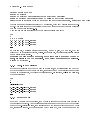
Here is a sample le (rst lines of the very standard iris data set) :
150
4
A B
5.1
4.9
4.7
...
C D
3.5
3.0
3.2
class
1.4 0.2 Iris-setosa
1.4 0.2 Iris-setosa
1.3 0.2 Iris-setosa
In this sample, 4 original attributes are given, named A,B, C and D. they are
followed by an additional attribute, class. In this sample, the original attributes consist
of numerical values (reals).
Remark: the user should be careful, not to leave empty spaces at the end of
lines, especially in the two rst lines. Such empty spaces might be misinterpreted by Explorer3D .
5.4.2
User-dened delimiter
If the space character might not be used as a delimiter, an additional line can be added
at the beginning of the le (on its 3rd line, thus after the number of attributes and before
the names of attributes), to declare the delimiter used. for instance, if | is the delimiter,
the le starts like:
150
4
|
A|B|C|D|class
5.1|3.5|1.4|0.2|Iris-setosa
4.9|3.0|1.4|0.2|Iris-setosa
4.7|3.2|1.3|0.2|Iris-setosa
...
5.4.3
Subset data le
If SUBSET is set on the rst line, then the le is supposed to contain only a subset of
the global set of objects. An additional numeric value must then be added at the begining
of each object-description line, that corresponds to the current object rank in the whole
set, starting at value 0. If the ranks given do not start at 0, then the user must use the
M. Exbrayat, L. Martin
8
optional parameter START WITH, followed by the oset. For instance, if his personnal
object numbering starts at 1, then he will write START WITH 1.
For instance:
SUBSET START WITH 1
3
4
A B C D classe
5 5.1 3.5 1.4 0.2 Iris-setosa
20 4.9 3.0 1.4 0.2 Iris-setosa
110 4.7 3.2 1.3 0.2 Iris-setosa
The user only gives 3 objects, with she has numbered 5, 20 and 110 in her own numbering
system that starts at 1. These objects are thus numbered 4, 19 and 109 in
5.4.4
Explorer3D .
How symbolic attributes are managed
Original attributes are by default supposed to be numerical (real). Symbolic values can
also be handeld.
Symbolic means that the values do not belong a continuous domain.
Thus, both integers and strings might be considered as symbolic attributes (integer will
be by default considered as numerical values unless they are be explicitly considered as
symbols).
Symbolic attributes will be denoted by a .S sux in their attribute name. Let us observe
the following example:
151
5
R1.S R2.S R3.S R4.S R5 Clas
A Green YES + 19 TRUE
B Red NO - 17 TRUE
C Blue NO - 49 FALSE
...
The rst four attributes are symbolic.
Concerning numerical attributes, their name can be suxed by .N, but this does remain
optional.
In the current implementation of
Explorer3D
a pre-processing is done on symbolic at-
tributes in order to binarize them: A rst scan of the column is done, in orderto list
the existing values of the attribute.
The unique attribute is then replaced by a list of
attributes (taking value 0 or 1), each one corresponding to a value of the symbolic one.
For a given object, all of these attributes are set to 0, except the one corresponding to
the original symbolic value. Such forged attributes are named as the original attribute,
rank,
except they are suxed by $
where
rank
is the rank of the symbolic value in the
list of existing ones.
for instance, in our example data set, R1 get replaced with two attributes, R1$1 and
R1$2, the values of which are respectively, for the rst object, 1 et 0, and for the second
object 0 and 1.
This decomposition is fully transparent to the user.
Explorer3D - User's manual
9
5.5 Distance les
Distance les contain distance matrices, i.e. matrices the elements of which correspond to
the distance between pairs of objects. The 3D view is then computed so that the distance
in the 3D space correspond as much as possible to the distances in the matrix. The le
inner format is as follows:
number of objects [COMPLETE]
distances between objects (one object per line)
[Number ou list of names of additional attributes
Values of additional attributes]
Where the squares braces denote optional parts.
By default, only the upper triangular part of the distance matrix is given: if we have 3
objects a, b and c, the rst line will contain
line
distanceab
and
distanceac ,
and the second
distancebc
On the rst line might occur the optional keyword COMPLETE, which means that the
distancea,a ,
distanceb,c , etc.).
full square matrix is given. According to our example, the rst line will contain
distancea,b
and
distancea,c ,
the second one
distanceb,a , distanceb,b
et
If additional attributes are given, and only their cardinality is given, their names are
automatically coined as follows: Att1, Att2, etc.
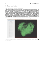
Here is a sample le (very rst lines of a inter-illumination distance matrix) :
166
...
1.0694574 1.1302139 1.0019832 1.0004523 ...
1.0656028 0.96607274 1.1858556 ...
...
image class
ms0001_1.jpg ms0001-Mazarine-Fr-SW-Début-12eme
ms0001_2.jpg ms0001-Mazarine-Fr-SW-Début-12eme
...
This data set consists of 166 objects. For each of them we have two additional attributes:
the name of an associated image le, and the name of the document the illumination
comes from.
the rst object belongs to document ms0001 - Mazarine - Fr - SW - Début 12eme, and
the user might nd a picture of the illumination in the le ms0001_1.jpg. The second
illumination comes from the same document and can be viewed in le ms0001_2.jpg.
The distance between the rst and the second object is 1.0694574; the distance between
the rst and the third object is 1.1302139; etc.
5.6 Raw 3D coordinates le
This kind of le does start by the number of objects it contains (it is computed automatically).
This might be reconsider in some future released of Explorer3D .
Optionnaly, the le might start by a line that contains the names of the 3 attributes.
Each remaining line contains the 3 coordinates (real values) of an object. These values
might be followed by additional attributes.
Here is a example le with three objects:
M. Exbrayat, L. Martin
10
0.5 0.5 0.5
-0.5 -0.5 -0.5
0 0 -2
5.6.1
Subset data le
Optionnaly, the keyword SUBSET should be added, alone on the rst line of the le.
Each remaining line will thus consist of four values, the rst one beeing the global rank of
each object. As with feature input les, SUBSET might be followed by START WITH
to specify an oset. for instance :
SUBSET START WITH 1
4 0.5 0.5 0.5
2 -0.5 -0.5 -0.5
1 0 0 -2
This le contains the coordinates of objects number 4, 2 and 1, with an oset of 1, that
is to say that the global rank of these objects are 3, 1 and 0.
5.7 Pure additional attributes les
the user can load les that consist of additional attributes with no projection data. Such
les are structured as feature input le, where the number of projection features is set to
0. Such les do only make sense in multisource mode.
5.8 Reserved attribute names (additional attributes)
Some reserved attribute names might be used, that are linked to a pre-dened visual
behaviour of
Explorer3D (i.e.
automatic object coloring, direct link to picture les), that
should normally be set by hand (see section 7.2.1). two names are currently reserved:
• ImgFileName :
the column contains picture le names. The path to les is relative
to the data le directory (e.g. concerning the data le in section 5.5, picture les are
supposed to be in the same directory as this data le). An absolute path can be set,
starting from the root directory (e.g.
/data/images/enluminures/img0001.png).
Pictures will be displayed either statically, on demand, on dynamically, when the
pointer passes over the corresponding object.
• Class :
a predened class for each object. In
Explorer3D , object class is displayed
by colouring objects. A class attribute can be either numerical or symbolic. The
Explorer3D
class-to-colour mapping is automatically set (
does nevertheless allow
the user to modify this mapping by hand).
5.9 Data import
If the data le inner format does not match
be executed.
Explorer3D
format, a data import tool can
This latter will be automatically loaded in case the user tries to load a
misformatted le. It can also be manually launched choosing the Files / Data import
Explorer3D - User's manual
11
tool menu. This wizard tool does allow to re-organize rows and columns and guides the
user step by step.
One must notice that only text (no binary les) feature input les
(neither distance matrices nor rax 3D coorindates) are currently supported.
This does
nevertheless cover most of needs. Do not hesitate to contact the authors in case additional
import features would be necessary.
To import spreadsheet data, please do rst save your le using the CVS (i.e. text) format,
and then open this le in the
6
Explorer3D import tool.
Visualisation interface: an Overview
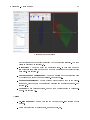
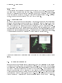
6.1 Handover
This section consists in a small tutorial on how to use
PCA.
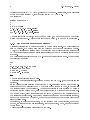
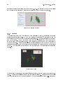
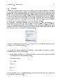
When starting
Figure 1:
Explorer3D
Explorer3D , the main control window opens (cf.
Explorer3D
main control window
in the context of a
g. 1).
Figure 2: PCA commands
(at launch time)
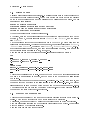
Let us rst load the data le. In the menu bar, let use choose Files / Load local le (new
project), and pick the
iris.csv le.
The main window aspect changes, so that it now oers
the functionnalities that are relevant to a feature le (also called the ND[imensions]
→
3D[imensions] perspective (see g. 2).
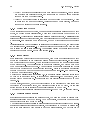
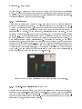
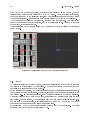
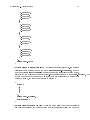
In order to compute a classical PCA, we rst check, in the Pre-treatments sub-window,
that Center variables is checked, and that Reduced variables is selected in the Reduction method list. Let us then click on Compute in the Projection Method sub-window.
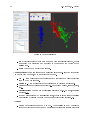
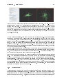
The 3D view then opens and displays objects using their default shape and colour, that
is blue spheres on a dark background (g. 3).
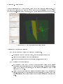
Let us now display an additional visual information, by the mean of object colouring
according to their class (each sphere correspond to a given kind of iris, and each kind of
M. Exbrayat, L. Martin
12
Figure 3: Default 3D view
iris belongs to one of three varieties). The class of a given iris (i.e. its variety) is stored
in an additional attribute, load together with the features, and named classe. Let us
display the sub-window Additional attributes by clicking on the upper-rigth arrows of
this sub-window, and let us choose classe in the Groups list (which is the only attribute
available, let-us ignore multigroups for the moment). spheres are then coloured and a
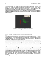
legend window pops up (g. 4).
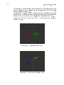
We can notice the presence of check boxes in the legend window.
The class check
boxes allow to display or hide the objects that belong to a given class. The Ellipsoid
checkboxes allow to display an ellipsoid around the corresponding group of objects (i.e.
the objects of a given class), that reects their spreading in space (g. 5) (Basically, this
ellipsoid is centered on the center of gravity of the group, and its diameters correspond
to the variance of the group along its three mains axes, based on the hypothesis of a
multinormal distribution). Figure 5 illustrate a visualisation of objects and the classes
ellipsoids.
One must notice that the top-line check boxes (blue background) are shortcuts to check
or uncheck the whole column.
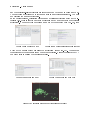
It is also possible to view the convex envelop of a group. This is done by checking boxes
in the Convex Envelop column. Figure 6 illustrates a 3D view where objects have been
hiden and only convex envelops are displayed.
Last, we can interact with the 3D view by using the three mouse buttons (left: rotation;
center: zoom; right: translation).
Explorer3D - User's manual
13
Figure 4: 3D View with colour and legend
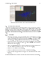
6.2 Control window menus
• Files:
data loading tools
Load local le:
allow to load the various supported kind of data les. The
le content is automatically discovered by
Explorer3D
. If no standard for-
mat is detected, an error message is displayed, and the data import tool is
automatically opened. Let us remind the three kind of data les managed by
Explorer3D :
∗
Feature les: the le is structured like a table where objects are described
by a set of numerical or symbolic features. 3D projection will be computed
by the mean of a dimensionnality reduction method (e.g. PCA).
∗
Distance matrix les: used when the only available data concern the distance or (di)similarity between objects. Projection will be computed by
the mean of a MDS.
∗
Raw 3D coordinates: when we directly get such data, for instance using
the output of another software.
Load online le:
this does permit to load a le stored on a distant machine,
on a HTTP server. The secondary that opens then allow to set the site URL
and then to explorer the web site directories. Supported le formats are the
same as for local les.
Data import tool: This tool allow to the content of a le text and to port it
to a Explorer3D -supported le format.
M. Exbrayat, L. Martin
14
Figure 5: Groups Ellipsoids
list of previously loaded les: once a le has been (succesfully)
memorized by Explorer3D and proposed to the user and the
Files menu.
Exit:
To shut down
• Perspectives:
loaded, it gets
bottom of the
Explorer3D cleanly.
This menu leads to some relevant sets of sub-windows with respect
to a given kind data le, or to a specic kind of task.
ND -> 3D:
Perspective that corresponds to features data les (projection
from N to 3 dimensions).
Distance -> 3D: Perspective that corresponds to distance matrix les.
Aspect:
Tuning of visual parameters (e.g. background colour, size of objects,
etc.).
Classication:
Oers a set of clustering algorithms (e.g. kmeans, gaussian
mixtures,...).
SVM: Oers various SVM visualisation tools, that is to says means to visualize
a separating hyperplan between two groups of objects (see section 8.6).
• Tools
:
Crop:
Data cropping based on a 3D box. This consisst in a way to select a
subset of objects and compute a new projection that limits to this set of objects
Explorer3D - User's manual
15
Figure 6: Convex envelops
and is optimal for that subset (according to the projection criteria). The crop
dialog is described in section 7.6.
Interaction:
A tool to modify the projection axes.
In this tool one set a
list of spatial anomalies and ask for a modied projection that corrects these
anomalies. See section 8.4
Travel thrgough dimensions:
A tool to manually set the projection axes
by chossing or mixing the axes available. See section 9.1.
Explore from images:
A tool to choose which objects to view in the projec-
tion space, together with the associated pictures and nearest neighbors. See
section 8.5.
Options:
To set various options, most of them corresponding to visual ele-
ments. See section 7.7.
• Help
On-line manual:
Opens a browser the browse the on-line version of this
manual.
About Explorer3D
: Version facts, mains authors, etc.
M. Exbrayat, L. Martin
16
7
Main functions
7.1 Projection methods
7.1.1
Based on a set of features
Projection method
Several techniques are currently proposed in the Projection Method
sub-window (reached through the Perspectives / ND -> 3D menu). The actual method
is chosen from a list. Currently available methods are:
• PCA
is the default method; it projects objects so that the distance between them
in the projection space corresponds as muh as possible to their distance in the
original space (input features are seen as coordinates in a high dimension space).
Two options are proposed with PCA:
dual auto and dual forced.
Roughly speaking,
the PCA dual method leads to the same projection as PCA, but can be much faster
when the number of input features is larger thet the number of objects. The user
must notice that dual projection forbids the future use of some complementary tools,
such as interactive projection.
dual auto compares the number of features and the
dual forced uses the dual
number of objects, and uses the dual method if needed.
method whatever.
• LDA
This method and all of the following ones rely on the availability of a class
attribute dened for each object. In other words, this supposes that an additional
attribute is available, that indicates the class of each object, and has been explicitely
set as the Groups attribute in the Additional attributes sub-window (see section
7.2.1). Projection is computed so that objects that belong to the same class tend
to be grouped, while objects that belong to dierent classes tend to be moved away
one from the other. This projection is computed in order to respect to some end
the original spatial distribution.
• R-discriminant Analysis similar to LDA, but only the interclass variance is maximized (it only focuses on moving away objects of dierent classes).
• Rw-discriminant analysis similar to r-discriminant analysis, but the original distance is also taken into account: the moving away of objects belonging to dierent
classes will be proportional to the inverse of the distance in the original space (i.e.
objects that are already far ont from the other in the original feature space will be
less aected than ones that were near one from the other). The sigma parameter
allows to tune the original distance impact.
The greater sigma, the smaller the
impact on originally distant objects (sigma=1 leads to a r-discriminant analysis).
• KNN PCA
• LLE
experimental - not documented
experimental - not documented
Pre-treatments
The Projection Method sub-window is tightly associated with the
Pre-treatment sub-window. This latter is used to apply to data a so-called conditioning.
This window oers various treatments to be done on data before applying the projection
method.
Explorer3D - User's manual
17
A check-box allows to choose wether data has to be centered or not. Centering means
that the values of each feature are translated so that their is zero. This pre-treatment has
to be done for ACP, and might be suitable for other method.
The data variance can be modied depending on the value chosen on the Reduction
method list: with
Raw data variance is not modied; with Reduced variables values
are rescaled so that the variance gets equal to 1 this option is suitable for PCA; with
Normalized distances
the values are rescaled so that the amplitude gets equal to 2,
and thus, together with data centering, values are between -1 and +1.
7.1.2
Based on a distance matrix
We currently propose a single projection method, which consists in a linear multidimensional scaling (MDS), that is a linear projection that computes 3D coordinates so that
the distances between pairs of projected objects do correspond as much to their distances
in the matrix.
Theoretically speaking, this projection stands if the input matrix does
really contain distances (with triangular inequality), in which case we can consider that
these distances were computed in a high-dimension space, and we thus make some kind
of dimensionality reducation. No pre-treatment is available.
We did recently had kernel methods. Those are presented in a specic section (8.7). Kernel
methods can be found in the kernel sub-window.
They allow for the computation of
non euclidean distances. For instance, using the isomap kernal, we will obtain a new
projection, were the only original distances that are kept in the projection space are
the ones between nearby objects (this kind of kernel is usually suited when the user
knows or guesses that objects are placed on the surface of some non plane surface (i.e. a
mathematical variety).
7.1.3
Based on 3D coordinates
In the case of 3D coordinates, projection is identical to input data. Centering and dimension dilatation are available (see section 7.4).
7.2 Using/displaying additional attributes
7.2.1
General Overview
Additional attributes are given as input but not directly used in the object spatial projection. They can for instance consist of the class of the object, an associated image le
name, etc. Five kinds of display modes are currently available:
• classes:
The selected attribute consists of the class of the objects. By default this
attribute is also used to colour objects (but colouring is not the only goal of the
class attribute). Fuzzy classes can also be visualized. In this case, each object is
supposed to belong to each group to a given level, the sum of these levels being
equal to 1. Fuzzy classes visualization is described in section 7.2.2.
• associated data:
In the current release, this function corresponds to the associated
images visualization;
• Label:
the textual value of the attribute is display in the projection space, near the
object;
M. Exbrayat, L. Martin
18
• Shape:
A specic shape is associated with each value of the attribute. Only a limited
set of shapes are currently avaible, and this should no be used with an attribute
taking more than 4 dierent values.
• Colour:
One dierent colour is associated with each value of the attribute. There
is no limit to the number of colours. Colouring can not be set directly, but can be
through the setting of the class attribute.
7.2.2
Multi Class Objects
When identifying groups of objects, the user can either associate a single group to each
object, or choose a fuzzy classication, where each object belongs to each group to a
certain level. While standard classication relies on a single attribute, multiclassication
numerical attributes, each one corresponding to the level of belonging to
In Explorer3D for a given object, the sum of these levels must be equals to
relies on several
a given class.
1.
Multiclassication can be visualized as follows: In the classes dropbox, the user chooses
the special value Multiclasses. A secondary list is then displayed in which the user
has to select the list of class attributes. The resulting display mode is similar to the one
describe in the fuzzy kmean-method (see section 8.3.3).
7.2.3
Image display
If an associated data attribute has been dened, then the image corresponding to each
object can be displayed on the basis of the le name stored in this attribute. Image display
can be either static or dynamic. Dynamic display occurs when the mouse pointer passes
over a given object. The corresponding image is then displayed, and hidden back when
the mouse pointer leaves the object. Dynamic display of images is optionanl and occurs
only if Show pictures when mouse is over is checked. Static image display is controled
through the popup menu that opens when the user makes a right-clic on a given object
with her mouse (see section 7.3.3).
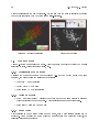
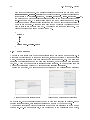
Depending on user's options (see section 7.7), image static display will occur either in the
3D view or in a specic window. If option Draw pictures out-of 3D is checked, then a
specic window is use (see g. 7); otherwise they are directly displayed in the 3D view
(see g. 8).
We can notice, in gure 7, that the objected linked to the pictures have been lected (red
background in the picture window, and highlighted color in the 3D view). We can also
notice that one image is currently dynamically displayed in the 3D view.
The default option consists in displaying images out-of the 3D view, in a spcic window.
7.2.4
Multiple picture sources
If several images are available for a single object, the user can decide to display them
simultaneously using a set of 3D scenes. To be more precise, the user can dene a specic
image attribute for each of her 3D scenes.
The default conguration consists in using a single image attribute for all of the 3D scenes.
If several additional attributes are available, that correspond to the name of picture les,
and if the user wishes to view a least two of them simultaneously, the way this can be
Explorer3D - User's manual
19
Figure 7: Out-of 3D scene (static) image
Figure 8: In 3D scene (static) image dis-
display + a dynamically displayed image
play. The corresponding object is at the
(mouse over the object).
upper left corner of the picture.
achieved with
Explorer3D consists in creating several 3D scenes, possibly using the same
projection, and then associating a specic image attribute to each of these scenes. For this
purpose, the user must rst activate the view a specic image attribute will be associated
with, then check the Specic A.D. box in the Additional attributes sub-window, and
last choose the specic picture attribute. Any scene for which the Specic A.D. box has
not been checked will use the global image attribute, if any has been dened. Conversely,
several scenes can use a specic image attribute.
Multiple picture sources can exist, for instance in the case multisource data, each of this
source bringing its own set of images, or more generally in the case images are just a side
information of the object studied and not the sources of features.
7.2.5
Management of colors
By default, colors are associated with classes, which means that setting a class attribute
implies that the same attribute is automatically set as the color one.
Nevertheless, it is possible to choose a color attribute directly, and thus to dissociate it
from the role of class attribute. This also allows gradient colouring (see g. 9). Gradient colouring is automatically used if the color attribute is of numerical type.
Explorer3D
Note :
does by default consider that additional atributes are of symbolic type. For
an additional attribute to be considered numerical, it must be explicitely declared as, in
the source le, its name being suxed with .N.
Colours can be replaced with black and white textures. The use of textures is activated
by checking the Texture box in the Additional attributes subwindow. There are currently ab. ten textures available. The user can change the texture associated with a set
of objects by clicking on it in the legend window. Textures are also displayed on ellipsoids
and convex envelopes if these laters are displayed.
Colours remain displayed, in the current release, to highlight selected objects (a selected
object will be coloured, even if textures are active; it be become textured again if deselected).
M. Exbrayat, L. Martin
20
Figure 10 illustrates the use of textures. We can see that the user is currently changing
the texture associated with the third group (iris-virginica).
Figure 9: Gradient coulouring
Figure 10: Textures
7.3 Mouse control
Using a 3-button mouse is recommended. Many tasks can be achieved throught he mouse:
selecting objects, displaying information, etc.
7.3.1
Manipulating the 3D scene
Pressing the mouse buttons on the background (i.e.
with no object under the mouse
pointer), the user obtains the following behaviours:
• Left press + move:
rotation
• Center press +move:
zoom
• Right button +move:
translation
7.3.2
Acting on objects
• Shift + left click:
select / deselect the object under the mouse pointer (a selected
object is highlighted in the scene). Object selection is used in several tasks.
• Right click:
7.3.3
Opens the popup menu
Popup Menu
Right clicking in the 3D scene opens a popup menu, form which various actions can be
achieved. When opening the menu while the mouse points on a projected objects, the
following ations are proposed:
Explorer3D - User's manual
•
21
Show / hide the picture associated with the object (if a picture attribute has been
dened);
•
Show / hide all pictures (same remark);
•
Show / hide the label associated with the object.
If no label attribute has been
dened, the object number is displayed;
•
Show / hide all labels;
•
Show / hide labels for the selected objects;
•
Make a spherical crop, centered on the currently pointed object. See section 7.6;
•
Make a planar selection. See section 7.4.1;
•
Center the scene on the currently pointed object;
•
Activate the magnifyer (see section 7.5).
If the menu is poped up while no object is pointed, only global actions are proposed
(global show / hide actions and planar selection).
7.4 Object selection
a uniform selection mecanism has been implemented. There exist several ways to get a
object selected: from the 3D scene, from the separated image windows, etc.
When an object gets selected in one of these views, in is also displayed as selected in the
other ones. For instance, when an object gets selected in the 3D scene, it gets highlighted
in this scene, but the corresponding picture (if displayed) does also get displayed on a red
background.
7.4.1
Multiple selection
Several objects can be selected at once. Choosing the planar selection in the popup menu
allow the user to draw a rectangle in the 3D view (clicking on the background a rst time
to set the upper left angle, and a second time to set the lower right angle of the rectangle,
see g. 11). All the objects within the rectangle get selected (see g. 12).
Figure 11: Multi selection (ongoing)
Figure 12: Multi slection (nished)
M. Exbrayat, L. Martin
22
7.5 Magnier
This tool, which can be activated through the popup menu, displays a leans in the 3D
scene, that magnies the objects under it. A very interesting side eect comes from the
fact that the magnied objects do also get selected. The user can thus see how objects
of a given view spread in other viws, if several are displayed.
Magnifying parameters
(diameter, coecient) can be adpted in the Magnier sub-window, which is displayed
when the Aspect perspective is chosen. Figure 13 illustrates the use of the magnier.
Figure 13: Magnier. In the left-most scene, selected objects are one that are magnied
(to be more precise, the ones that are under the magnier) in the right-most scene. One
can notice the magnier parameters sub-window, in the control window.
7.6 Crop
Crop consists in choosing a subset of the objects displayed and then to compute a new
projection and scene that ts this subset. The resulting projection can be quite dierent
from the original one.
There are two ways to crop:
• Box crop the selection zone is a box.
Such a crop is initiated from the Tools/crop
menu, which displays a crop dialog. Clicking on New Crop is this dialog, a cubic
box gets displayed, that is centered at the origin of the scene.
This box can be
moved and /or resized using the sliders in the crop dialog (g. 14). S If objects
were selected when New crop is clicked, then the box is automatically sized and
moved to contain these objects.
When the bow has resized and moved as suited, clicking on Crop! causes a new
dataset to be produced, that contains the croped object, and a new projection and
3D scene to be computed. Croped view can be croped in turn, and so on.
• Spherical crop
This crop zone is centered on a given object (g. 15). Such a crop
is accessed through the 3D scene popup menu;
Explorer3D - User's manual
23
Figure 14: Box crop
Figure 15: Sperical crop
7.7 Options
The option window is accessed through the Tools/options menu. The current options
are:
• Default color
of the objects: The cvoloured rectangle can be clicked, in order to
modify this default colour;
• Enhancement of 3rd dimension at display time:
When the 3D scene gets
displayed, a slight rotation is applied, so that the 3 projections axes get visible;
• Display original axes:
projection sub-space.
Original axes (i.e.
input features) get displayed in the
This option aectes only feature-based projections.
This
action should moved away from the option list in a further release.
• Draw pictures out-of 3D window:
to choose whether statically displayed pic-
tures get displayed in the 3D scene or in a separate window (default value);
• Autocompute 3D projection:
If not checked, the user has to choose and launch
a projection technique once data has been loaded. Otherwise, the projection and
3D scene are automatically computed. In case of a feature data source, the default
projection technique is PCA.
• Activate distant execution:
this option should be checked in case the user wants
to display the 3D scene on an image wall. This old option has not been maintained
in the recent releases and should not be used.
• Show source data (array):
to display in a table the values of additional attributes
(see section 8.2).
• Show picture when mouse is over:
controls the dynamic display of pictures in
the 3D scene (see section 7.2.1).
• Activate stereo if available:
If the graphical card (and screen) of the computer
support stereoscopic viewing, then stereo gets activated.
M. Exbrayat, L. Martin
24
• Size of labels:
a slider to set the size of labels in 3D scenes;
• Dynamic object size:
If checked, object size is computed depending on the num-
ber of number to display (the larger the number of objects, the smaller their individual size). If checked, then Size of objects is not available.
• Size of objects:
A slider to manually set the default object size.
• Multisource mode:
Allow the user to manipulate multi source data sets (see 5.2).
• Network command available:
If checked, then
Explorer3D listens on a port (by
default, port 50000) for some commands. The protocol and available commands are
presented in section 8.9.
• Port number:
to manually set the network command port. Currently unavailable.
• Legend available:
If unchecked, the legend window is not displayed.
Legend
windows and their functionalities are presented in section 7.8.
Figure 16: Options
7.8 Legend
Depending on the object colouring policy, the legend window displayed will vary.
The
standard legend window (one colour per object, a nite set of colours) as already been
presented in section 6.1. Two others kinds of legend windows are available: the multiclass
legend window and the continuous colour attribute legend window.
7.8.1
Multiclass legend window
This legend window is displayed when multiclassication is active. This occurs when the
user does manually set a multi-class system (see section 7.2.2) or when a fuzzy classication tool is used (see section 8.3.3).
belong at most. Due to
Objects ar coulored according to the class they
Explorer3D current evolutions, additional actions proposed by
Explorer3D - User's manual
25
this legend window are not currently fully functional; nevertheless, the user can visualize
the centroïd of each group (appears as a small cross, coloured as the group). Class diffusion through objects can also be observed using convex envelops: by checking activate
convex envelops and moving the bottom slider, envelop either dilate or shrink to the
objects that belong to the class at a higher level than the one indicated by the slider. The
ellipsoïd column is not currently used.
Figure 17: Multiclass legend window. Here we observe a fuzzy kmeans. Each objetct is
coloured according to its main class.
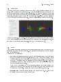
7.8.2
Continuous attribute legend window
The user can dene a colouring that does not rely on a given (set of ) class(es), but rather
on a single, numerical (oating point) attribute.
A colour gradation is then computed
to handle any value of the chosen attrifute, from the smallest one to the largest one (see
gure 18).
Each object gets coloured depending on the attribute value it is associated
with. Such a colouring technique is not chosen through the additional attributes subwindow.
This colouring technique can be activate by three kinds of actions: selection
of an explicitely numerical additional attribute as colouring attribute; SVM visualization
using colour to materialize the distance of the object to the separating hyperplan (see
section 8.6); and materialization of a fourth projection axis by the mean of colouring (see
section 7.9). This legend window does only contain the gradation together the min and
max values of the attribute.
M. Exbrayat, L. Martin
26
Figure 18: Continuous attribute legend. On can notice that the colouring corresponds to
a fourth axis materialization, that in fact is the same as x1.
7.8.3
Texture-based legend
As introduced in section 7.2.5, colours can be replaced by textures. The legend will allow
the user to identify and possibly modify the texture associated with a given group.
7.9 Projection axes
The Projection axes sub-window allow several actions on the 3D scene. The two rst
proposed actions are:
• Zoom on less discriminative dimensions
: depending on the projection tech-
nique, it might frequently occur that objects get well spread along x1, but more
concentrated along x2 and even more on x3. To get a better dispersion in the scene
the user might check this optionin order to dilate object coordinate on the less
exploited axes (see gure 19).
• Center cloud
:
this option translates the objects so that the origin does not
correspond to the baryceeter any more but to the median value along each axis.
This two options do apply to the current scene and to the ones that are computed afterwards.
Explorer3D - User's manual
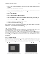
27
Figure 19: Zoom on less discriminative dimensions et cloud centering. The left-most scene
corresponds to a basic PCA projection, the right-most one to the PCA where the two
options have been used. The scenes have been rotated so that axes x2 and x3 can be well
observed. We can see that objects get more spreaded along x3 in the right-most scene
than in the left-most one (this can be also observe, while less important, along x2) and
that the object cloud has been translated to the left (centering) compared to the one in
the left-most scene.
A third action is available, that alow to choose the projection axes. This functionnality
does only make sense when at least three axes are available, that is to say with a nD>3D projection, based on feature input data. Nevertheless, the user can always choose at
least to invert the dimension-to-axes mapping, or to use the same dimension along several
axes. The user can specify the projection dimension used on each axes, in the following
order: x1 (breadth), x2 (heigth) and x3 (depth). The scene is only modied once the user
clicks on Draw. This manually-set projection does not generate a new scene, but rather
move objects in the current scene.
The dimensions available are numbered from 1 to n (these are the dimensions computed by
the projectin method, not the raw input features). An additional value is given, denoted
X, which indicates that the corresponding axis is not used. For instance setting x3 to
X means that objects with all be placed in the x1-x2 plan.
Last, we can choose a projection dimension to colour object (continuous attribute colouring).
The coulouring dimensions can be chosen among the projection dimensions com-
puted by the projection method (not among the raw features; this might proposed in a
further release). Checking the Colouring dimension box, the user activates the continuous attribute colouring, based on the dimension value of each object. Figure 18 illustrates
the dimension-based colouring. We can see in this gure that we used the same dimension
for colouring as the one used to project objects along x1. Nevertheless, any other available
projection dimension might have been used.
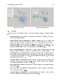
7.10 Observations
This sub-window indicates the amount of original variance that is displayed using the 3
current projection dimensions (gure 20). a histogramm gives the amount of variance each
available projection dimension brings; currently used projection dimensions are drawn red,
unused ones are drawn blue. A pie-chart chart gives the amount of original variance that
M. Exbrayat, L. Martin
28
the current scene oers.
If a class attribute has been selected, then a class purity index is displayed at the bottom
of the sub-window (Dunn index).
Figure 20: Observations sub-window. We can notice that many projection dimensions
are available. The three most signicant have been chosen for the 3D display (red bars
of the histogram), and that they support 49.5 % of the original variance (pie-chart). A
class attribute has been selected (the quality of which is displayed, according to the Dunn
index).
7.11 Project save and load
The user can save the current project, in order to reload it later.
The current saving
strategy manages data sources, 3D scenes, and the active additional attributes (class,
colours, etc.).
To save the current project, choose Save project in the Files menu. To load a project,
choose Load project.
Projects are by default saved with the .e3d le extension. Technically speaking, they
consist of text les using the JSON format.
8
Main tools
8.1 Multi-view visualization
Explorer3D is oriented towards a multi-scene interactive use.
This can be used to follow
several goals: rst to open several visualization windows simultaneously, and second to
observe the behaviour of a set of selected objects in these various windows.
8.1.1
Multi-view principle
The term view does mainly correspond to the 3d scene window. It also corresponds to
less used windows, such as tables or 2D graphs. The user can compute and manipulate
several 3D scenes for a unique dataset, mainly to:
•
observe the same projection under several points of view;
•
observe dierent projections on a unique dataset (PCA, LDA, etc.);
•
observe both a global view and one or several crops.
Explorer3D - User's manual
8.1.2
29
How controls aect 3D scenes
Some control have a global eect on 3D scenes; colouring is currently one of them (mainly
to identify the of classes in several scenes). Conversely, many control are not supposed to
have a global eect, and rather a local one on a single 3D scene; this stands for clustering,
crops, etc.
For this purpose we introduce the notion of
active
view: the
active
view is the one that
is aected by the execution of a non global control action. How can we set and highlight
the
active view?
A view can be set active by giving the focus to its window Once the view has been set
active, the window border gets red (see gure 21). A view remains active until another
one is set active, either explicitely or implicitly. For instance, computing a new 3D scene
makes it active. Only one view at most is active at any time.
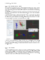
Figure 21: Several simultaneous views.
The active view (bottom-right) can be identi-
ed by its red border. We can notice that global controls have been used on the views
(colouring according to classes), as well as local controls (the lightgrey background of the
upper-left scene)
8.1.3
View browser
The set of available views can be browsed in the View Exlorer sub-window. This subwindow contains a tree-view of the current state of explorer3D, with data input les (data
sources) as roots, followed by the projection method, the projection (axes) and nally the
view (usually: the 3D scene). The currently active view is highlighted in this browser.
Clicking on a given view in the browser gives makes it active.
M. Exbrayat, L. Martin
30
Figure 22 presents the view browser. We can notice that we currently use an attributevalue (feature set) data source, on which we computed a PCA and used the 3 main
axes of this latter to compute the 3D scene. We can also observe that we used another
projection method, were the 3rd projection axis is set to -1, which means that the x3
(z) axis is not used.
Figure 22: View browser. An Attribut / Value (feature set) data source has been used,
on which both a PCA and a LDA have been computed. A crop has been computed on
one of these views (there is a secondary data source, that is a child of the rst one). The
crop-based scene is currently active (grey background).
8.1.4
Selected objects in views
Selected objects are highlighted in the 3D scenes. The set of selected objects is global to
all views. This means that selecting an object in one view highlights it in all the views.
This can be usefull to look for a given (set of ) object(s) throughout several views.
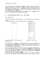
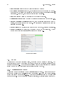
8.2 Tabular view of objects
Options allow the user to view a table that contains the additional attributes for the
current object set As dened previously, additional attributes consist of data that are not
used to compute the object projection, but rather to bring additional knowledge on the
objects.
This table contains all of the objects sorted according to their index number. By default,
all additional attributes are available. Whether each attribute is displayed can be chosen
Column visibility/ additional attributes menu. Projection coorbe displayed using the column visibility / projection coordinates
by the mean of the
dinates can also
menu. By default, projection coordinates are not displayed.
Object selection is availale in this table, and the set of objects displayed can be limited
to the selected ones (see g. 23). for this purpose, check Filter (selection) in the Lines
visibility menu.
For more details on the selection mechanism, please see section 7.4 .
8.3 Clustering
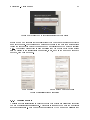
Several clustering methods are available. They can be reached by choosing the Classication perspective (see g.24) in the main window menu. Several of the proposed method
Explorer3D - User's manual
31
Figure 23: Tabular view of additional attributes (with lter)
shared a common weakness: they are fully stable (they do not always produce exactly the
same set of groups). For this reason we encourage the user to compute them several times
(using the recompute button) to ensure a good understanding of the methods stability
w.r.t.
the current dataset (let us also underline that the Recompute button should
also be pressed if the classication parameters, if any, such as the number of groups to
produce, have been modied).
when opening
once a method has been chosen
Figure 24: classication perspective
8.3.1
Gaussian mixture
Gaussian mixture classication is built on the idea that objects are distributed according
to a ste of multivariate gaussian laws. A technique is thus use to compute the most likely
set of underlying laws. Each computed law is displayed by the mean of an ellipsoid that
M. Exbrayat, L. Martin
32
is centered oriented and sized as the law (see g. 25). The current method (which relies
on the klustakwik algorithm) does automatically compute the number of laws.
Figure 25: Gaussian mixture
8.3.2
Kmeans
The principle under that very standard hard clustering method, consists in producing
clusters of similar diameters. To be more precise, this algorithm minimizes the sum of
the distance of each object to the nearest cluster center. The user rst sets the expected
number of groups. Group Centers are then randomly initialized and each object is put
in to the group of the nearest center. Each center is then updated to the barycenter of
the group objects. This process is iterated until stabilization (or a maximum number of
iterations is reached).
In our current implementation, the default number of centers is
set to 5. The user can modify this number and recompute the corresponding clustering
result.
Figure 26: Kmeans
Kmeans being not stable, an additional tool is proposed, that computes the stable components. This tool is accessible through the stables subwindow. a stable is a set of object
that are always put in the same cluster by a given clustering method (i.e. kmeans in
Explorer3D - User's manual
33
our software). By always we mean in any of a given number of runs of the clustering
method. In this tool we can choose the number of classes and also the number of runs to
be conducted. Once the runs have all been done, the resulting set of stables is displayed.
Stables are currently computed for kmeans only.
8.3.3
Fuzzy kmeans
This method is derived from the former one, where each object now belongs to all of the
groups at a certain level (degree).
The degree is related to the distanceto the center.
The sum of degrees is equal to 1. Here again the user can choose the number of centers
(default: 5). On one hand, the interest behind this method is to leave more freedom of
interpretation to the user. On the other hand, visualization is bit more tricky. We thus
developed a specic technic, based on convex envelops, that we did already partly present
in section 7.8. Two kinds of information has to be displayed : rst, the main group of
an object, and second the set of objects that belong to a group to a given degree. The
main class is displayed using a classical legend. Concerning the degree, we use convex
envelops (see g. 27): for each group (or a set of groups) we display the set of objects that
belong to it to a certain degree, i.e. for which the degree of belonging is higher that x
percent (remind that we assume that the sum of degrees is 1). The current value of the
x threshold can be set using a slider, and the evolution of envelops can thus be observed
dynamically. One can notice that this tool can also be used when a fuzzy classication is
given as an input and thus coming from a third-tier tool.
Figure 27: Fuzzy kmeans visualization with convex envelops and threshold.
8.3.4
Density-based classication (DBSCAN)
Diering from the former methods, that rely on the distance to a given group center, and
thus lead to spherically-structured groups, density-based methods build groups starting
from the dense parts of the objects space.
Objects are then aggregated in groups de-
pending on their neighboorhood (diusion). Such methods are relevant when objects are
structured in dense, arbitrary shaped groups.
M. Exbrayat, L. Martin
34
Two parameters can be manually set: rst the neighborhood radius (the maximum distance within which two objects are considered as neighbors), and the minimum group
cardinality (how many neighbors are needed at least to form a group). In order to help
the user to set the radius, a sphere is displayed at the enter of the 3D scene.
Figure 28 presents the result of a DBSCAN clustering. We can notice that the rst group
consists of the isolated objects (i.e. the ones that do not belong to a cluster). This group
might be empty.
Figure 28: Density-based classication (dbscan)
8.3.5
Minimal spanning tree and hierarchical classication
The minimum spanning tree is a tree that links the objects displayed. Briey speaking,
this tree links each object to its nearest neighbor, starting from the nearest pair of objects).
Visualising this tree shows how objects are linked from near to near.
A long link will
highlight the existence of two distant groups, etc.
A hierarchical classication consists in grouping objects starting from the nearest ones,
always adding the nearest remaining one, which might be either a object or an already
formed group. There exists several ways to compute the distance between two groups.
The one we use is called minimal jump: The distance between an object and a group
is the distance between the object and the object opf the group that is the nearest to
him. Between two groups, it is the minimum distance between two objects that belong
to each of the group respectively. We produce a classication tree, called dendrogram.
Dendrograms are very common, for instance to classify species. While they are usually
display in a at manner, we propose to view them directly in the 3D scene (see g. 29).
The reader might notice the strong link between the minimum spanning tree and the
hierarchical classication based on minimal jump. The number of clusters to be formed
is set by the user. Forming the groups does simply correspond to cut the tree at a certain
level, starting from the root, where the number of branches equals the expected number
of groups.
Explorer3D - User's manual
35
Figure 29: Minimal spanning tree et hierarchical classication
8.4 Spatial reconguration
This tool is an experimental one the user is encouraged to test. This tool can be reached
through the Tools/Interaction menu.
It allows to set a list of relative distance con-
straints, in order to ask for objects to be moved closer or far away, and to modify the
projection dimensions in order to respect these constraints as much as possible while introducing as few global distorsion as possible. We rts invite the user to try the Comparison
tool.
8.4.1
•
Comparison
First check the Object A box, and then click on any object within the 3D scene.
A red target is then displayed around this object (g. 30). A green target is also
displayed that surround the second object (the one the distance to object A should
be modied). By default, this second object is the object with global rank 0.
•
Check the Object B box and click on the second object, i.e. the one you really
want to move away or nearer to object A. T green target is moved in order to
surround this object (g. 30).
•
Using the horizontal slider, set the expected distance: to the left, objects have to
be moved closer; to the right they have to be moved away (g. 30).
•
Click on OK to validate your constraint.
•
Click on Run ! in order to compute the new projection dimensions.
•
When computing is over, targets get hidden, and the projection space gets modied
(g. 31).
Several constraints should be entered and taken into account for a space modication.
M. Exbrayat, L. Martin
36
Figure 30: Distance constraints: The two objects concerned can be identied in the 3D
scene (object A-41 :red target; object B-98 : green target). The constraint asks for the two
objects to be moved closer (slider in the left-most window, and the constraint is textually
displayed in the bottom-left list (Comp | 41-98 < 0.85...)
Figure 31:
Distance constraints:
the constraint has been integrated in the projection
framework. We can see that projection has been modied and that the two objects are
now closer.
8.4.2
Anomaly
The Anomaly tool allow the user to modify the relative positionning of three objects.
We thus manipulate three objects A, B and C. The underlying idea consists in modifying
distance A-C with regards to distance A-B. In other words, the user expect C to be moved
close to or away from A so that in becomes closer or more far away from A than B.
We proceed as before, using the checkboxes and the scene to set A, B and C and then
modifying the distance rate using the slider.
Explorer3D - User's manual
8.4.3
37
Move
The underlying idea consists in changing the neighborhood of an object. This is a rather
complex method the user might use with care. The user must rst set the target neighborhood by selecting the objects that belong to it, and then by clicking on Add. She
must then click on object to move, and click on the corresponding object.
Just like
before, the user than has to click on OK and then on Run !.
8.4.4
Observation axis
In order to observe a subset of objects along a given axis, the user can set observations
axes. For this purpose, the user chooses the Observation Axis tab (g. 32), and then
chooses to objects to from the ends of the axis (by clicking on them in the 3D scene). The
number of objects to be displayed is then set (default: 10), and the user clicks on OK.
The 10 objects that are the nearest ones to the segment are then selected, and a table
containing informatin about these objects (global rank and additional attributes) is then
displayed (Objects description window). Several axes can be available simultaneously.
The user selects the ones to be displayed / hidden using the Axis: window.
Figure 32: Displaying an observation axis: we observe the ten nearest objects to axis
8-14.
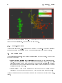
8.5 Explore from Images
In order to make the projection space more readable, we add the possibility to only display
a subset of the objects, based on the associated pictures. For this tool to work properly,
the associated data additional attribute must have been set. The user then activates
the tool by checking Explore from Images in the Tools menu.
All objects are then
removed (hidden) from the 3D scene and a new window, Associated pictures opens,
where the user can choose the objects he wants to display (g. 33). The user then chooses
the pictures he wants to observe, either in the drop-down list available at the top of the
window (List tab + validate) or by typing the picture le name (Name tab + validate).
M. Exbrayat, L. Martin
38
Each time a new picture is choosen, this picture gets displayed in the window, and the
corresponding objects is set visible back in the 3D scene. When a picture gets clicked,
the object is swaped to the selected state, and the corresponding shape in the 3D scene
becomes haighlighted. Clicking again on a picture causes the object to be deselected.
The object n neighbors can be displayed, together with their picture. the value of n
is set by the user in the Neighbors tab, and is by default set to 0. When an object gets
hidden back, so are its neighbors.
This explroation can be superimposed with the standard dynamic display of pictures in
the 3D scene.
Figure 33: Explore from images (with 5 nearest neighbors)
8.6 SVM
SVM stands for support vector machine, which are a classication tool that try to separate
two groups of objects using a (hyper)plane. They are thus usable when the user knows
the class of at least a subset of the objects.
In the easiest conguration, the separation is a plane in the original or projection space,
that perfectly separates the groups. Moreover, this plane must be as far as possible of the
two groups (i.e. as central as possible). Such a clear separation is not always available.
Either the groups might be somehow mixed, or separated by a surface that does not look
like a plane. For this reason, SVM are usually used together with kernels (see section 8.7).
If more that two groups exist, it is possible either to dene a SVM between two of the
groups or between one group and all the remaining ones.
In
Explorer3D
the SVM control are accessed through the SVM perspective. The class
attribute must have been set before using SVMs.
Explorer3D - User's manual
39
Figure 34 illustrates a SVM simple case, based on the very standard iris dataset. We
can see that a plane has been drawn in the 3D scence that materializes a SVM computed
between the iris-setosa group on one side, and the remaining groups on the other side.
Figure 34: SVM with separating plane (iris dataset)
Availables commands are as follows:
•
•
SVM subwindow: to dened the groups to be separated.
constant: do not modify this value, which is currently unused (1);
rst group: one class among the available ones
second group: either one of the remaining class, or all of them;
SVM Display Mode subwindow:
computation mode: the SVM can be computed either based on the orginal
dimensions (input features) or on the projection space. An original dimensionbased SVM will be more accurate, but it will not be possible to draw it as a
plane in the 3D scene.
display mode: the simplest and easiest to interpret display mode consists of a
plane.Nevertheless, two additional modes are available, that allow some kind
of materialization when plane display is not possible coloring et replace 3rd
axis.
M. Exbrayat, L. Martin
40
The colouring mode uses a colour grade to recolor the objects relatively to their
side and distance to the hyperplane (red on one side, green on the other one).
Figure 35 illustrates this mode.
the replace 3rd axis used the x3 projection axis to materialize the side and
distance to the hyperplane for each object. Projection based on input features
is then limited to the x1 and x2 axes. Figure 36 illustrates this mode.
Theses two modes can be used with both SVM computed in the original or
projected space.
Figure 35: SVM coloring display mode
Figure 36: SVM with 3rd axis display mode
Explorer3D - User's manual
41
8.7 Kernels
Kernels are powerful tools that have been widely used in machin learning due originally
to SVM. As we said before, identied an separating hyperplane is not always easy nor
feasible both in the original and projected space. Kernels compute new attributes based
on some combinations of the original ones. Most of these combinations are not linear, but
must anyway respect some criterias. The trick with kernels is that in fact they all allow
to compute a distance between object without really computing the new attributes, and
thus propose various and potentially complex spaces at a low cost. We invite the reader
to consult the abundant bibliography of the eld for more details.
In
Explorer3D
kernels are available in the SVM and ND->3D perspectives.
The
Kernels subwindow allow the user to select a given kernel in a drop-down list and
to set the potential parameters of that kernel.
Once a kernel has been choosen , it is
applied on any new peojection (click on the Compute button of the Projection Methode
subwindow to apply the kernel to the current scene).
Figure 37:
kernel control subwindow.
We can see that a polynomial kernel has been
choosen, with a degree 2 polynom.
We just list the kernels available in
Explorer3D
and encourage the reader to refer to
kernels litterature to get more details:
•
linear kernel: this is dummy kernel that allows the user to keep using the original
dimension space while kernels are active.
•
polynomial kernel
•
RBF kernel
•
Sigmoid
•
Isomap
•
LLE
Even not kowing much on their specicities, the newby user might test them, looking for
an interesting projection space.
M. Exbrayat, L. Martin
42
8.8 2D Graphs
The 2D Curves subwindow allow the user to use various additional curves:
• Shepard diagram this diagram highlights the link between distances in the original
and projection spaces.
• 2D (symboles) and 2D (labels) produce the same projection as a 3D scene, using
only the two rst axes. The
its class. The
Symboles mode displays each object using the shape of
labels mode display the objects labels (by default, their rank).
• Contributions
• Square cos
• Voronoi cells
These tools are supposed to help interpreting the 3D scene.
they
rely on a snapshot of the scene, in which the Voronoi cell around each object is
computed. We remind to the user that Voronoi celle in the portion of space that
is nearer to a given object (point in the space) than to any other object. The cells
coloring depends on the kind of visualisation:
Proximity tells how far objects are
in the original space from a given object. The user must select a single object in
the 3D scene before opening this kind of graph;
Distorsion
tells how much the
distance between two neighbors has been aected by the 3D projection. Distorsions
do not rely on Voronoi cells, but on Delaunay triangle, which are complementary to
Voronoi cells. Neighbors in the 2D graph are linked by a quadrilateral the colour of
which runs from white (no distorsion) to black (strong distorsion).
Proximity and distorsion graphs can be used to compare 2D and 3D projections,
2D projections and ND (original space), 3D projections and ND.
These tools might not be fully functional currently.
8.9 Network-driven control
This tool allow the user to connect a third-tier software to
Explorer3D
, in order to
visualize objects and additional data coming from this third-tier software. This function
gets activated through the option window (see section 7.7).
Explorer3D
then listens on
a given port (currently port 50 000), and waits for text commands sent using the json
format.
The list of commands available is quite simple for the moment, and focus on receiving
a set of objects features et on setting or updating their class (and, by the way, their
colouring)
• loading objects
in the message:
: objects are described by a set of features. Their are two parts
the command name (``msg'':''set-data''), then the objects
description ("val"
: [ [object1], [object2], ...]).
4 objects described by four features:
{
"val": [
[
Here is an example with
Explorer3D - User's manual
],
[
],
[
],
[
]
}
43
0.09995818,
0.8450656,
0.31611204,
0.9885413
0.20870173,
0.6817836,
0.30197513,
0.20966005
0.95933825,
0.7643002,
0.23336774,
0.7409621
0.075930595,
0.12991834,
0.6995411,
0.092056274
],
"msg": "set-data"
• objects class denition (full set) :
The class of all objects is given. the message
consists of three parts: the command name (``msg'':''set-classes''), then the
number of classes (``nbclasses'':
value) and last the class value for each object,
: [ [classe_object1], [cl
sorted in the same order as objects in the set-data message ("val"
Here is an example with our set of 4 objects: there are 2 classes; the 3 rst objects
belong to class 1, the fourth one belongs to class 0 :
{
}
"val": [
1,
1,
1,
0
],
"msg": "set-classes",
"nbclasses": 2
• objects class denition (subset)
some given objects and
: this command allows to change the class of
can only be invoked after the global class setting command has
M. Exbrayat, L. Martin
44
been invoked at least once.
The message consists of two parts: the command name
(``msg'':''set-classes-fast'') and the list of changes. This latter consists of a
table ("val"
: [ [classe_object1], [classe_object2], [jump_objects], ...]),
the encoding of which is as follows: values ar sorted as the objects appeared in the
set-data command.
A positive value stands for a new class value of the corre-
sponding object; a negative value indicates a jump in the set (objects the class of
which is not modied). Here is an example with our 4 objects; The class of the two
rst objects is not modied (jump 2). The class of the third one is set to 0. The
class of the fourth one is not modied (jump 1).
{
}
"val": [
-2,
0,
-1
],
"msg": "set-classes-fast"
8.10 Data import
The data import tool is open when the user tries to laod a le with an unknown format. It
might also be directly open to format an input le, through the Files / Data import tool
menu. This rather intuitive tool does rst load the source le (g. 38). The user then
indicates the delimiters used in the le: eld separator, dot symbol and text separator
(g. 39). A view of the input le is available during this step. In the proposed example
we use the Parkinson dataset (UC Irvine machine learning repository).
During the next step, the source le is cut according to the delimiters and presented
Figure 38: Import: initial window
Figure 39: Import: setting delimiters
as a table (g. 40); the user indicates the kind of data that is stored in this le. In the
current implementation, only feature sets les are managed by the import tool.
The user then indicates whether the features of an object are organized as a row or as a
column (g. 41). In our example le, a row correspond to the description of an object,
Explorer3D - User's manual
45
and the projection-relevant features are stored in rows 2 to 196 and in columns 2 to 24.
The rst column contains the object names (this is an additional attribute).
The rst
row contains the names of attributes.
In the current release, description features and additional attributes might not be interlaced (i.e. there is exactly one block of features and at most one block of additional
attributes). The import then proposes a summary of the imported data (g. 42), then
Figure 40: Import: data type
a view of the nal imported le using the
Figure 41: Import: description of le content
Explorer3D
format (g. 43).
The user can
then either save the le or save it and compute a projection. Figure 44 presents the PCA
computed after importing the Parkinson dataset.
Figure 42: Import: summary
Figure 43: Import: end of import
Figure 44: Projection after import (Parkinson dataset)
M. Exbrayat, L. Martin
46
9
Secondary tools
9.1 Travel throughout dimensions
This tool can be reached through the Tools / Travel throughout dimensions menu. It
allows the user to manually set the three projection dimensions by mixing the projection
dimensions computed by the system (ND -> 3D mode). The content of each axis is set
by the mean of sliders, each slider corresponding to an available projection dimensions.
Clicking the Draw button causes the objects to move smoothly to their new coordinates
(see gures 45 to 47).
The most simple use of this tool is quite similar to the one of-
fered by the Projection axes subwindow of the 3D->ND perspective (see section 7.9).
Nevertheless, using this secondary tool, the user can compute any mix of dimensions, for
instance summing the values of several dimensions on the x3 axis.
Figure 45: Travel throughout dimensions:objects are projected on the three main projection dimensions.
Explorer3D - User's manual
47
Figure 46: Travel throughout dimensions: we choose to replace the third dimension with
the fourth on axis x3.
Figure 47: Travel throughout dimensions: after the axis modication.
Index
2D graphs, 40
colouring, 25
manually mixing, 44
Active view, 27
Additional attributes, 15
Sheppard diagram, 40
SVM, 36
Colouring
gradient, 17
View browser, 27
texture, 17
Voronoi cells, 40
Colouring dimension, 25
Continuous attribute legend window, 23
Zoom on less discriminative dimensions, 24
Crop
box, 20
spherical, 20
Data conditioning, 14
Data import, 42
Hierarchical classication, 32
Interactive projection
anomaly, 34
comparison, 33
move, 35
observation axis, 35
Kernels, 39
Linear discriminant analysis, 14
Magnier, 20
Minimum spanning tree, 32
Multiclass legend window, 22
Multidimensionnel scaling (MDS), 15
Objects Cloud (centering), 24
Observations, 25
Options, 21
pré-traitements, 9
Pre-treatment, 14
Principal Component Analysis, 14
Projection
3D coordinates, 15
distance matrix -> 3D, 15
ND -> 3D, 14
Projection axes, 24
choose, 25
48