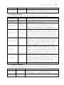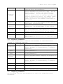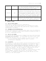
1
CDPOP user manual |1 CDPOP USER MANUAL 2011 Version: 1.0 Authors: E. L. Landguth1, B. K. Hand1, J. M. Glassy1,2, S. A. Cushman3 and M. Jacobi1 1 - University of Montana, Division of Biological Sciences, Missoula, MT, 59812, USA. 2 - Lupine Logic Inc, Missoula, MT, 59802, USA. 3 - U.S. Forest Service, Rocky Mountain Research Station, 2500 S. Pine Knoll Dr., Flagstaff, AZ 86001, USA CDPOP user manual |2 Table of Contents 1 2 3 4 5 6 7 Introduction.................................................. 3 1.1 Changes from CDPOP v0.7............................... 3 1.2 What can CDPOP do..................................... 3 1.3 How does CDPOP work................................... 3 Getting started............................................... 5 2.1 Dependencies.......................................... 5 2.1.1 Baseline requirements............................ 5 2.1.2 Python on non-windows platforms.................. 6 2.1.3 Python on windows................................ 6 2.1.4 Obtaining NumPy and SciPy........................ 6 2.2 Installation.......................................... 6 2.2.1 Installing Python, NumPy, and SciPy.............. 6 2.2.2 Unpack the CDPOP archive........................ 7 2.2.3 Install CDPOP................................... 7 2.2.4 Description of CDPOP files...................... 7 2.3 Example run........................................... 7 2.3.1 Command line run................................. 8 2.3.1 GUI run.......................................... 9 Input......................................................... 9 3.1 Input Files........................................... 9 3.2 Model Parameters...................................... 10 3.3 Mating Parameters..................................... 10 3.4 Dispersal Parameters.................................. 11 3.5 Offspring Parameters.................................. 11 3.6 Genetic Parameters.................................... 12 3.7 CDEVOLVE.............................................. 12 3.8 CDINFECT.............................................. 13 3.9 CDCLIMATE............................................. 14 Output........................................................ 14 General issues................................................ 15 5.1 How to obtain CDPOP.................................. 15 5.2 Debugging and troubleshooting......................... 15 5.3 How to cite CDPOP.................................... 15 References.................................................... 16 Acknowledgements.............................................. 17 CDPOP user manual |3 1 Introduction The goal of this user manual is to explain the technical aspects of the current release of the CDPOP program. CDPOP v1.0 is a major extension of the CDPOP program (Landguth and Cushman 2010). CDPOP is an individual-based program that simulates the influences of landscape structure on emergence of spatial patterns in population genetic data as functions of individual-based movement, breeding, and dispersal. 1.1 Changes from CDPOP v0.7 There are major innovations in v1.0 which were not included in the previously published v0.70. We list below the new functionalities of CDPOP v1.0: 1.2 Natural selection is implemented through differential offspring viability as functions of fitness landscapes. Gene flow and natural selection can now be simulated in dynamic landscapes. A graphical user interface provides a user friendly platform that enables users to explore, analyze, and model the effects of lifehistory and differential models of complex landscapes on the genetic structure of populations. Sex-specific dispersal. Module driver plug-in architecture. Changes of some internal software components have allowed an overall speed increase and to improve program stability. Additional movement function option: negative exponential movement. Inclusion of both a mating landscape and a dispersal landscape. Vertical transmission of an infection. mtDNA option. Output genotype option in a general genetic format. What can CDPOP do CDPOP‟s realistic representation of the spatial environment and population genetic processes provide a powerful framework to investigate the impact of ecological factors on the genetic structure of populations. This approach has already advanced knowledge of the patterns of genetic variation in spatially-explicit contexts (Landguth et al 2010a; Landguth et al 2010b; Cushman and Landguth 2010). Example simulations have included: Quantifying the time to detect barriers. Correlate migration rates and landscape resistance barriers. Testing for the effects of population sample size and number of markers. CDPOP user manual |4 1.3 How does CDPOP work CDPOP v1.0 models genetic exchange for a given resistance surface and n – (x, y) located individuals as functions of individual-based movement through mating and dispersal, vital dynamics, and mutation. A user must specify the input parameters through a graphical user interface or input script file. As the model simulates stochastic processes, most applications will quantify mean and variability of genetic structure across many runs. Thus, a Monte Carlo option is provided for the user to choose the number of runs to simulate given a single set of input parameters. In addition, a user may also frequently wish to launch several runs with different parameter values simultaneously (i.e., sensitivity analysis). This functionality is provided through batch capability. The simulation program assumes constant population density over time. Individuals are assumed to occupy a fixed grid on the landscape that is user defined by the n - (x,y) located individuals. The genotype of each locus for each individual can be initialized by randomly choosing from a file containing allele frequencies for each locus, or by reading in a file containing the initial multi-locus genotypes of all the individuals. The initial age structure of the population is specified by an input file specifying initial age frequency. The sex of each initial individual is randomly assigned. There are five movement functions that define how individuals choose a mate and disperse on the landscape as a function of cost distance: linear, inverse square, negative exponential, nearest-neighbor, and random mixing. With the nearest-neighbor movement function, an individual moves to the available grid location nearest its initial location. Random mixing moves an individual to a grid location that is randomly chosen from the n grids in the population. In linear, inverse-square, and negative exponential movement functions, individuals move a distance from their initial location based on a draw from a probability distribution inversely proportional to a linear, inverse-square, or negative exponential function. The user specifies the maximum dispersal distance (in cost units) an individual can travel on the landscape. The probability is one at no distance from the original location and goes to zero at the maximum dispersal distance. Reproduction is defined by the user as either hermaphroditic or heterosexual. With hermaphroditic mating, there are no distinct sexes, but individuals mate with other individuals according to the movement function choice, exchanging genes in Mendelian reproduction. In heterosexual reproduction, mated pairs are one male to possibly many or no females, and the end of the mating process occurs when all females have mated. Each mated pair can have a number of offspring that is a bounded random draw based on a uniform probability distribution, a Poisson draw with specified mean, or a constant number. Mendelian inheritance with k-allele mutation (rate chosen by the user) is used to generate the offspring‟s genotype and the sex CDPOP user manual |5 assignment is random. Dispersal of offspring occurs from according to the selected movement individual. The vital rates (birth the population will have emigrants the mother‟s (x,y) location function and the sex of the and death) define whether or not or immigrants. Simulating natural selection. Past versions of CDPOP modeled three sources of genetic variation: gene flow, genetic drift, and mutation. These versions assumed that different genotypes have an equal probability of surviving and passing on their alleles to future generations and thus, natural selection was not operating. CDPOP V 1.0 implements natural selection analogously to the adaptive or fitness landscape of allele frequencies (Wright 1932). This new functionality enables extension of landscape genetic analyses to explicitly investigate the links between gene flow and selection in complex landscapes at an individual‟s level. The user specifies fitness landscape surfaces for each genotype of a single diallelic locus that is under selection. For example, three relative fitness surfaces must be specified for the three genotypes, AA, Aa, and aa, from the two alleles, A and a. Selection is implemented through differential survival of dispersing individuals as a function of the relative fitness at the location on that surface where the dispersing individual settles. CDPOP v1.0 reads and extracts genotype and location specific fitness values for each n – (x, y) individual in the pre-processing step. The program will continue all other processes the same as CDPOP, with an additional step implement selection during the dispersal process. Simulating dynamic landscapes. The potential impacts of climate change on the connectivity of populations have become an area of concern among scientists and land managers. Current needs include quantitative and spatially-explicit predictions of current and potential future patterns of fragmentation under a range of climate change scenarios (Opdam & Wascher 2003). To address this need, CDPOP v1.0 allows users to input a new landscape surface at a given generation time through new cost distance matrices for both mating and dispersal. The program is written in Python 2.6 and provided with installation instructions for most platforms, along with sample input files. CDPOP v1.0 is built on a driver-module, plug-in, docking architecture that allows for ease of future modular development. CDPOP v1.0 has been debugged as carefully as possible by testing all combinations of simulation options. Information for users, including user manual, FAQ, publications, ongoing research, developer involvement, and downloads can be found at http://cel.dbs.umt.edu/software/CDPOP/. 2 2.1 Getting started Dependencies CDPOP user manual |6 2.1.1 Baseline Requirements CDPOP requires the Python2.6.x interpreter, NumPy package, and SciPy package. Remember that Python modules usually require particular Python interpreters, so be sure the version ID for any external Python module or package (e.g. NumPy or others) matches the version of your Python interpreter (normally v2.6.x). 2.1.2 Python on Non-Windows Platforms Some common computer platforms come with Python installed. These include MAC OS X and most Linux distributions. To determine which Python a MAC or Linux workstation has installed, start a terminal console and enter “python.” You'll see the version number on the top line (enter Control-D to exit). Replacing an older Python interpreter (pre v2.4) with a newer one (v.2.6.x) on a Linux or MAC OS X machine can be tricky, so ask a System Administrator for help if you‟re not sure which packages depend on the current Python installed. 2.1.3 Python on Windows Windows (7, XP, 2000, Server) does not come with Python installed, so follow the instructions below to obtain and install Python on a computer running the Windows operating system. Get a windows installation of the base Python installation (current v.2.6.x) at: http://www.python.org/download/releases/. 2.1.4 Obtaining NumPy and SciPy We recommend using the superpack Windows installer available from the SourceForge website: http://sourceforge.net/project/. Note that more complete information for NumPy is available at www.scipy.org, where the SciPy module is also presented. Another source is http://www.enthought.com/products/epd.php for a free academic and educational usage in a single downloadable installer that has everything and then some (Numpy, Scipy, Matplotlib, and 70+ modules for python). 2.2 Installation 2.2.1 Install Python, NumPy, and SciPy Make sure that Python and NumPy are installed, and available to you. You can test this by typing "python" at a command window. If python is available you'll get the python prompt ">>>". If it is not a recognized command, it means either that python is installed but is not in your command shell's paths, or that python is not installed. In the first case ask an administrator to add it to your command paths. If your shell locates and loads python, type, "import numpy". Similarly, type, “import scipy”. If python does not complain that there are no such modules, all is well. The following instructions assume Python, NumPy, and SciPy are not yet available on your computer; if they are, skip to section 2.2.2. * First run the Python executable installer you've chosen (either from www.python.org or ActiveState, accepting defaults for the installation CDPOP user manual |7 directory. On Windows this will typically place the executables and libraries in c:/Python2.6/bin and the "site-packages" package tree for user installed Python modules in c:/Python2.6/lib/site-packages. If you are installing it on a network on which you do not have administrative privileges, you may need to ask a system administrator to install python and the NumPy and SciPy packages in their default locations. * Next install NumPy and SciPy using the supplied executable (superpack) installer or visiting http://www.scipy.org/Download. This will install NumPy and SciPy in your Python ./site-packages directory. 2.2.2 Unpack the CDPOP Archive Navigate to the directory on your PC where you wish to install CDPOP, and unpack the supplied zip archive file using a free archive tool like 7Zip (7z.exe), Pkunzip, Unzip, or an equivalent. Seven-Zip (7Z.exe) is highly recommended since it can handle all common formats on Windows, MAC OS X and Linux. On Windows, it is best to setup a project specific modeling subdirectory to perform your modeling outside of any folder that has spaces in its name (like "My Documents"). 2.2.3 Install CDPOP Next, install the CDPOP software itself by unpacking the zip archive supplied. At this point you should be able to execute the supplied test inputs. 2.2.4 Description of CDPOP files 20 files will be installed in your directory. Here is a description of each: README.txt – a quick how to run CDPOP instructions CDTable16.csv - example N-(x,y) for the cost distance matrix EDcdmatrix16.csv - example Euclidean distance cost distance matrix xyED16.csv – example n-(x,y) for individuals CDPOP.py - Python driver code and run file CDPOP_Disperse.py - Python library for the dispersal functions CDPOP_GetMetrics.py - Python library for the metric functions CDPOP_Mate.py - Python library of the mating functions CDPOP_Modules.py - Python library with general functions CDPOP_Offspring.py - Python library for the offspring functions CDPOP_PostProcess.py - Python post-processing library CDPOP_PreProcess.py - Python pre-processing library cdpopi.py - GUI python file to run CDPOP.py agedistribution.csv – example age distribution file allelefrequency.csv – example allele frequency distribution file fitvals0.txt – example fitness landscape for offspring selection fitvals1.txt – example fitness landscape for fecundity selection fitvals100.txt – example fitness landscape for adult selection inputvariables.csv – run parameters corresponding to the example files RipMgr.py - installation file for package RipMgr CDPOP user manual |8 2.3 Example run 2.3.1 Command line run The example run is for 16-points representing individuals with a Euclidean distance cost distance matrix. To run the following example, follow these steps: 1. Double check that the twenty files provided in the archive are in the same directory. Make a note of this directory name, which we will call the home directory (for example, I would save all of the archive information in a location named, C:/CDPOP/ExampleRun). 2. The included file inputvaribles.csv specifies the parameters that can be changed and used in a sample CDPOP run. Open inputvaribles.csv in your editor of choice. A spreadsheet program like Microsoft Excel, allows for easy editing of the tabular values. 3. There will be 3 lines of information in inputvariables.csv: a header line and 2 lines of information corresponding to 2 separate CDPOP runs (batch process). Section 3 contains a breakdown for each column header and the parameters that can be changed. The Input listed is for the first row in the file. You will need to *CHANGE* the Directory column‟s information to your home directory as noted in Step 1. For example, I would change text in A2 and A3 using Excel to point to my home directory for this example run to read C:/CDPOP/ExampleRun/. BE SURE to remember to put the final forward slash at the end of the path name. 4. After you have made the home directory change in step 3, save inputvariables in the same format – inputvariables.csv, a comma delimited file. Select „Yes‟ or „OK‟ for any Excel questions about saving in this format. 5. Start the program with a graphical interface or at the command line: For example, if you downloaded Python 2.6.x from www.python.org, then you are provided with a graphical interface, IDLE. In Windows you can find IDLE from your Start menu > All Programs > Python 2.6 > IDLE (Python GUI). Alternatively, if you use python from the command line, then open a terminal window and change your shell directory to the CDPOP home directory. 6. Run the program: There are a number of ways to run this program. In IDLE, open CDPOP.py by going to File > Open, then browsing to your home directory, clicking on CDPOP.py, and OK. A new window will appear with CDPOP.py source code. In the menu bar, click Run > Run Module. If you are using a command shell you can run the program by typing “python CDPOP.py”. 7. Check for successful model run completion: The program will provide stepby-step output in the Shell window. Once completed, a simulation time will be printed out and folders batchrun0mcrun0, batchrun1mcrun0, and batchrun1mcrun1 will be created in your CDPOP home directory to store output from the separate batch and/or Monte-Carlo runs. Each of these folders will have a unique date/time stamp preceding „batchrun0mcrun0‟ in case you want to run multiple CDPOP runs in this same directory. The CDPOP user manual |9 program will also provide a log file with program steps in your CDPOP home directory. 2.3.2 GUI Run The following are instructions for a simulation run with an optional graphical user interface (GUI). Note that this GUI has a dependency on python library, WX python. Go to http://wxpython.org/download.php and download your OS‟s version of WX python. 1. Navigate to CDPOP folder and double click cdpopi.py. 2. Enter in values for each variable. To find out more information on a specific variable, click the radio button to the right of the variable label. 3. After all values are entered; click the Submit button at the bottom. If a value is in the wrong format, you will be notified at the bottom. 4. The program is running successfully if the command prompt opens up and displays text related to running CDPOP and output folders created in your directory. 3 Input 3.1 Input files The following are the general input files used in CDPOP. provided for formatting. File Header Example Directory *CHANGE* Xyfilename xyED16 agefilename N Matecdmatrixfilename EDcdmatrix16 Dispcdmatrixfilename EDcdmatrix16 See examples Description Home directory location of all CDPOP files. Change this to match the pathname of the location of all CDPOP files. Make sure to include the final forward slash at the end of the pathname. The n-(x,y) grid location values. This is a comma delimited file with 5 column headings: a unique identifier (FID), x-coordinate location (XCOORD), y-coordinate location (YCOORD), a string label identifier (ID), and an initial sex assignment (sex). See xyED16.csv for an example xyfilename. The distribution that is used to initialize the model‟s n individuals‟ age structure. If N is entered, then this file is not used. If a filename is entered, then read in the file (for example agedistribution would be entered for the example provided). See the agedistribution.csv for formatting this file. A [NxN] cost distance matrix for mating movement, where N >= n and n is the number of grid values (or individuals) on the landscape. This is a comma delimited file. A [NxN] cost distance matrix for dispersal movement, where N >= n and n is the number of grid values (or individuals) on the landscape. C D P O P u s e r m a n u a l | 10 Xycdmatrixfilename CDTable16 This is a comma delimited file. The N-(x,y) coordinate values for both the mating and dispersal cost distance matrices. This is a comma delimited file with a header row (X,Y). 3.2 Model parameters The following list are the model parameters used for CDPOP. File Header Example Mcruns 1 Looptime 5 Nthfile_choice Sequence Nthfile_List 0|3|4 Nthfile_Seq 1 Panans N Twopopans N Oldmortperc 100 Description The repeated number of simulations to be conducted for the Monte Carlo method. Simulation run time [generation]. File output indexed from 0 – (looptime-1). The choice of a specified simulation run time to write to file and to calculate genetic distance matrices. If List is entered, then read nthfile_list values below. If Sequence is entered, then read nthfile_seq value below. The specified simulation run time to write to file and to calculate genetic distance matrices. These values are used if nthfile_choice = List. These values must be separated with a vertical bar. Note that maximum value in Nthfile_List must be Looptime – 1 due to indexing starting at 0. The specified simulation run time to write to file and to calculate genetic distance matrices. This value is used if nthfile_choice = Sequence. This is the „by‟ value in the sequence. For example 1 would create values starting at 0, ending at looptime-1, by every 1 generation. Use this parameter to specify whether or not there is panmixia in your populations. For example, your resistance surface may include a barrier that separates populations that include panmixia on either side. This allows you to include random movement with landscape effects. Possible values to enter are N and Y. Use this parameter with panans = Y to test two populations that are separated by a landscape feature, and follow random movement within their respective populations. This is for a specific set of simulations that assumes only two populations in your study. Possible values to enter are N and Y. Percent mortality in the adult population. 3.3 Mating parameters The following lists the parameters used for the movement of individuals due to mating. File Header Example Matemoveno 1 MatemoveparA 1 Description Movement function answer for mating. 1 = Linear, 2 = Inverse Square, 3 = Nearest Neighbor, 4 = Random Mixing, 5 = Negative Exponential. This is only used for negative exponential y = a*10^-bx and is the parameter a. C D P O P u s e r m a n u a l | 11 MatemoveparB 1 Matemovethresh 5 Freplace N Mreplace Y Selfans N Sexans Y Reproage 0 This is only used for negative exponential y = a*10^-bx and is the parameter b. A threshold option (in cost distance units) for how far an individual can search for a mate. You can specify „max‟ to consider all individuals for mating movement. You can also place a integer value in front of „max‟ to consider a percent cost distance movement for mating. For example „10max‟ would consider all mating individuals that are within 10 percent of the maximum cost distance on the surface. If you want females to mate with replacement, then specify „Y‟. If you want females to mate without replacement, then specify „N‟. If you want males to mate with replacement, then specify „Y‟. If you want males to mate without replacement, then specify „N‟. If you want to allowing selfing (i.e., individuals mate with themselves), then specify „Y‟. If you do not want to allow for selfing, then specify „N‟. „Y‟ for sexual reproduction and „N‟ for asexual reproduction. The age at which individuals can reproduce. Use with overlapping generations, i.e, oldmortperc not set to 100. 3.4 Dispersal parameters Here lists the parameters used for the movement of individuals with regards to offspring dispersal. File Header Example Fdispmoveno 2 FdispmoveparA FdispmoveparB 1 1 Fdispmovethresh 5 Mdispmoveno 1 MdispmoveparA MdispmoveparB Mdispmovethresh 1 1 10 Description This is the function answer for female movement for dispersal. 1 = Linear, 2 = Inverse Square, 3 = Nearest Neighbor, 4 = Random Mixing, 5 = Negative Exponetial. Used only for negative exponential y = a*10^-bx and is the parameter a. Used only for negative exponential y = a*10^-bx and is the parameter b. A threshold option (in cost distance units) for how far an individual female offspring can disperse on the landscape. This is the function answer for male movement for dispersal. 1 = Linear, 2 = Inverse Square, 3 = Nearest Neighbor, 4 = Random Mixing, 5 = Negative Exponential. Used only for negative exponential y = a*10^-bx and is the parameter a. Used only for negative exponential y = a*10^-bx and is the parameter b. A threshold option (in cost distance units) for how far an individual male offspring can disperse. 3.5 Offspring parameters The following list are the parameters to deal with offspring births and deaths. C D P O P u s e r m a n u a l | 12 File Header Example Offno 2 Lmbda 5 Femalepercent 50 Equalsexratio Y newmortperc 0 Description This is the litter size or the number of offspring each mate pair can have. Choose 1 for a random draw, 2 for Poisson draw, and 3 for a constant number of offspring for each mother. The parameter value used with offno. If offno = 1, then lmbda is the max range value between 0 – lmbda to draw randomly from. If offno = 2, then lmbda is the Poisson mean for the litter size. If offno = 3, then lmbda is the constant litter size value. Percent number of female born in each litter. The answer to have every generation start with equal sex ratios. Possible options include „N‟ and „Y‟. Percent mortality in the offspring population. 3.6 Genetic parameters The following lists the parameters associated with the initialization of the genotypes, mutation rates, and mtDNA option. File Header Example Geneswapgen 0 Muterate Loci 0.0005 10 Intgenesans random Allefreqfilename N Alleles 10 mtDNA N Description The generation time that genetic information is exchanged. The k-allele model mutation rate. The number of loci. The choice for how to initialize the genotype for each n-(x,y) individuals. If „random‟ is entered, then the genotypes get a random assignment and the population is at a maximum genetic diversity. If „file‟ is entered, then the genetics get drawn from the allele frequency distribution file (specified in next column, allefreqfilename). If „known‟ is entered, then the genotypes are directly read from a given known file. Email Erin Landguth for an example file to use for „Known‟. The allele frequency distribution for each locus, used to initialize the model‟s n individual‟s genotype. If „N‟ is entered, then this file is not used. If you want to use a frequency distribution file, you must set intgenesans to equal „file‟ and then enter in the filename in this field. See allelefrequency.csv example file for formatting this file. The number of alleles per locus. If „Y‟, then last locus becomes mtDNA and every offspring inherits this locus from its mother only. If „N‟, then regular Mendal inheritance occurs. 3.7 CDEVOLVE The following lists the parameters and selection surfaces used to simulate natural selection. File Header Example Description C D P O P u s e r m a n u a l | 13 Cdevolve N AdultMortFit Fitvals100.t xt OffspringMortFitAA Fitvals0.txt OffspringMortFitAa Fitvals0.txt OffspringMortFitaa Fitvals0.txt Fecundity Fitvals1.txt This is the selection answer. „Y‟ or „N‟ response to turn on CDEVOLVE, natural selection. Alleles must be 2 if „Y‟ is entered. This is the adult viability selection surface. If adult has AA or Aa, then this mortality fitness surface is used, which increases the individual‟s chance of survival if oldmortperc > this fitness surface value. Oldmortperc is used for individuals that have aa. To turn this selection function off when cdevolve = „Y‟, then set oldmortperc == this fitness surface. This is the offspring viability selection surface for AA. If offspring has AA, then this mortality fitness surface is used, which increases the individual‟s chance of survival if newmortperc > this fitness surface value. Newmortperc is used for offspring that have Aa or aa. To turn this selection function off when cdevolve = „Y‟, then set newmortperc == this fitness surface mortality value. This is the offspring viability selection surface for Aa. If offspring has Aa, then this mortality fitness surface is used, which increases the individual‟s chance of survival if newmortperc > this fitness surface value. Newmortperc is used for offspring that have AA or aa. To turn this selection function off when cdevolve = „Y‟, then set newmortperc == this fitness surface mortality value. This is the offspring viability selection surface for aa. If offspring has aa, then this mortality fitness surface is used, which increases the individual‟s chance of survival if newmortperc > this fitness surface value. Newmortperc is used for offspring that have AA or Aa. To turn this selection function off when cdevolve = „Y‟, then set newmortperc == this fitness surface mortality value. This is the fecundity selection surface. Fecundity surface is proportion of offspring for aa. Use with constant offspring at set level, e.g. offno == 3 and lambda == 10 would produce 10 offspring for every mother with AA and Aa. Then the Fecundity selection is performed for individuals with aa and fitness surface at proportion of set offspring level (eg 0.10 would produce 1 offspring for every mother with aa). 3.8 CDINFECT These parameters are used with the module CDINFECT. Currently only vertical transmission is assumed. Future development will include horizontal transmission parameters. File Header Example CDInfect N Description This is the infection parameter answer. This tracks vertical transmission in the population. If „Y‟, then a random status infection (0 or 1) C D P O P u s e r m a n u a l | 14 Transmission prob 0.5 is created and initialized for each individual. If „N‟, then the status 0 is created for all individuals and initialized. A column in grid.csv denotes the infection status at each generation for every individual. This is the transmission probability for if a parent has the infection the chance that the infection will be passed along to the offspring. 3.9 CDCLIMATE These are the parameters that control the dynamic landscape functionality within CDPOP. A generation time is specified and input cost distance matrices are then read into the program and used in simulations. File Header Example CDClimate N CDclimgentime 10 Futurematecdmat EDcdmatrix16 Futuredispcdmat EDcdmatrix16 Description This is the dynamic landscape answer. If „Y‟, then a new cost distance matrix will be read in at a specified generation time in next column. The generation time that the new cost distance matrix will be read in at. A [NxN] future cost distance matrix for mating movement, where N >= n and n is the number of grid values (or individuals) on the landscape. This is a comma delimited file format. Note that this file must be the same size as the initial cost distance matrices used in the simulations. A [NxN] future cost distance matrix for dispersal movement, where N>= n and n is the number of grid values (or individuals) on the landscape. This is a comma delimited file format. Note that this file must be the same size as the initial cost distance matrices used in the simulations. 4 Output The following is a list of output options from CDPOP, including options to calculate cost distance matrices, Euclidean distance matrix, genetic distance matrices, and genotype formatting. File Header Example MateCDmatans N DispCDmatans N Description This is the mating cost distance matrix answer. If „Y‟, then the cost distance matrix used for the n grid locations is extracted from the N mating cost distance matrix locations. If „N‟ is entered, this matrix is not created. Note that currently only the initial cost distance matrix is used to create this matrix, not the futurematecdmat. This is the dispersal cost distance matrix answer. If „Y‟, then the cost distance matrix used for the n grid locations is extracted from the N dispersal cost distance locations. If „N‟ is entered, then this matrix is not created. Note that only the initial cost distance matrix is used to create this dispersal cost distance matrix, not the futuredispcdmat. C D P O P u s e r m a n u a l | 15 5 Edmatans N Gendmatans Dps Gridformat General This is the Euclidean distance matrix answer. If „Y‟, then the Euclidean distance matrix used for the n grid locations is calculated. It „N‟ is entered, then this matrix is not created. This is the genetic distance matrix answer. The genetic distance matrix used for the n grid locations for specified generation time of the simulation run is calculated. Enter „braycurtis‟ for the Bray-Curtis distance measure, „Dps‟ for the proportion of shared alleles, or „Da‟ for Nei‟s genetic distance. Note that Nei‟s genetic distance takes the longest to calculate and may decrease your total CDPOP simulation time. This is the genotype output format option. The format for the genotype output is specified by entering „general‟ for a general genotype output or „cdpop‟ for the cdpop genotype output. General issues 5.1 How to obtain CDPOP The program is freeware and can be downloaded at http://cel.dbs.umt.edu/software/CDPOP/ with information for users, including manual instructions, FAQ, publications, ongoing research, and developer involvement. 5.2 Debugging and troubleshooting For help with installation problems please check first for postings at our web site. Otherwise, please report problems including any bugs, to me at [email protected]. 5.3 How to cite CDPOP This program was developed by Erin Landguth with help from Brian Hand, Joe Glassy, and Sam Cushman. GUI development was done by Mike Jacobi. The reference to cite is: Landguth EL, Hand BK, Glassy JM, Cushman SA, Jacobi M (2011) CDPOP v1.0: An individual-based landscape genetics program. Bioinformatics. Submitted. 5.4 Disclaimer The software is in the public domain, and the recipient may not assert any proprietary rights thereto nor represent it to anyone as other than a University of Montana-produced program (version 1.x). CDPOP is provided "as is" without warranty of any kind, including, but not limited to, the implied warranties of merchantability and fitness for a particular purpose. The user assumes all responsibility for the accuracy and suitability of this program for a specific application. In no event will the authors or the University be liable for any damages, including lost profits, lost savings, or other incidental or consequential damages arising from the use of or the inability to use this program. C D P O P u s e r m a n u a l | 16 We strongly urge you to read the entire documentation before ever running CDPOP. We wish to remind users that we are not in the commercial software marketing business. We are scientists who recognized the need for a tool like CDPOP to assist us in our research on landscape ecology issues. Therefore, we do not wish to spend a great deal of time consulting on trivial matters concerning the use of CDPOP. However, we do recognize an obligation to provide some level of information support. Of course, we welcome and encourage your criticisms and suggestions about the program at all times. We will welcome questions about how to run CDPOP or interpret the output only after you have read the entire documentation. This is only fair and will eliminate many trivial questions. Finally, we are always interested in learning about how others have applied CDPOP in ecological investigation and management application. Therefore, we encourage you to contact us and describe your application after using CDPOP. We hope that CDPOP is of great assistance in your work and we look forward to hearing about your applications. 6 References Allendorf,F.W. and Luikart,G. (2007) Conservation and the genetics of populations. Blackwell, Malden, MA. Bowcock,A.M. et al. (1994) High resolution of human evolutionary trees with polymorphic micorsatellites. Nature. 368, 455-457. Cushman,S.A. et al. (2006) Gene Flow in Complex Landscapes: Testing Multiple Hypotheses with Casual Modeling. The American Naturalist 168, 486-499. Cushman,S.A. and Landguth,E.L. (2010) Spurious correlations and inferences in landscape genetics. Molecular Ecology, 19, 35923602. Holderegger,R. and Wagner,H.H. (2006) A brief guide to Landscape Genetics. Landscape Ecology 21, 793-796. Landguth,E.L. and Cushman,S.A. (2010) CDPOP: A spatially-explicit cost distance population genetics program, Molecular Ecology Resources, 10, 156-161. Landguth,E.L. et al. (2010a) Quantifying the lag time to detect barriers in landscape genetics. Molecular Ecology, 19, 4179-4191. Landguth,E.L. et al. (2010b) Relationships between migration rates and landscape resistance assessed using individual-based simulations. Molecular Ecology Resources, 10, 854-862. Legendre,P. and Legendre,L. (1998) Numerical ecology. 2nd English ed. Elsevier,Amsterdam. McRae,B.H. and Beier,P. (2007) Circuit theory predicts gene flow in plant and animal populations. Proceedings of the National Academy of Science USA 104, 19885-19890. Nei,M. et al. (1983) Accuracy of estimated phylogenetic trees from molecular data. Journal of Molecular Evolution 19,153–170. Ray,N. (2005) PATHMATRIX: a GIS tool to compute effective distances among samples. Molecular Ecology Notes 5, 177-180. Storfer,A. et al. (2010) Landscape genetics: where are we now? Molecular Ecology, 19,3496–3514. C D P O P u s e r m a n u a l | 17 Wright,S. (1932) The roles of mutation, inbreeding, crossbreeding, and selection in evolution, Proceedings XI International Congress of Genetics, 1, 356-366. 7 Acknowledgements This research was supported in part by funds provided by the Rocky Mountain Research Station, Forest Service, U.S. Department of Agriculture and by the National Science Foundation grant #DGE-0504628.