Download HORNET User Manual - Computation Structures Group

HORNET User Manual
Copyright © 2011 MIT
LIST OF FIGURES
CONTENTS
Contents
1
Introduction
2
Getting Started
2.1 Before Installation . . . . . . . . . . . . .
2.2 HORNET Design Overview . . . . . . .
2.2.1 Simulating registered hardware
2.2.2 Tile-based system model . . . .
2.2.3 The PE and the bridge . . . . . .
2.2.4 The network switch node . . . .
2.3 How to Install . . . . . . . . . . . . . . .
2.4 Generating a System Image File . . . . .
2.5 Running a Simulation . . . . . . . . . .
3
1
.
.
.
.
.
.
.
.
.
.
.
.
.
.
.
.
.
.
.
.
.
.
.
.
.
.
.
.
.
.
.
.
.
.
.
.
.
.
.
.
.
.
.
.
.
.
.
.
.
.
.
.
.
.
.
.
.
.
.
.
.
.
.
.
.
.
.
.
.
.
.
.
.
.
.
.
.
.
.
.
.
.
.
.
.
.
.
.
.
.
.
.
.
.
.
.
.
.
.
.
.
.
.
.
.
.
.
.
.
.
.
.
.
.
.
.
.
.
.
.
.
.
.
.
.
.
.
.
.
.
.
.
.
.
.
.
.
.
.
.
.
.
.
.
.
.
.
.
.
.
.
.
.
.
.
.
.
.
.
.
.
.
.
.
.
.
.
.
.
.
.
.
.
.
.
.
.
.
.
.
.
.
.
.
.
.
.
.
.
.
.
.
.
.
.
.
.
.
.
.
.
.
.
.
.
.
.
.
.
.
.
.
.
.
.
.
.
.
.
.
.
.
.
.
.
.
.
.
.
.
.
.
.
.
.
.
.
.
.
.
.
.
.
.
.
.
.
.
.
.
.
.
.
.
.
.
.
.
.
.
.
.
.
.
.
.
.
.
.
.
.
.
.
.
.
.
.
.
.
1
1
1
1
1
2
2
3
4
4
Configuring Your System
3.1 Running a Synthetic Network Traffic using a Trace-driven Injector (Network-Only Mode) . .
3.1.1 XY Routing on an 8x8 2D Mesh with 2 virtual channels . . . . . . . . . . . . . . . . .
3.1.2 Trace Format (writing an event file) . . . . . . . . . . . . . . . . . . . . . . . . . . . . .
3.1.3 Changing Routing Algorithms . . . . . . . . . . . . . . . . . . . . . . . . . . . . . . . .
3.1.4 Changing the Number of Virtual Channels . . . . . . . . . . . . . . . . . . . . . . . . .
3.1.5 Changing Virtual Channel Allocation Schemes . . . . . . . . . . . . . . . . . . . . . .
3.1.6 Using Bidirectional Links . . . . . . . . . . . . . . . . . . . . . . . . . . . . . . . . . . .
3.2 Running an Instrumented Application (native x86 executables) using the Pin Instrumentation Tool . . . . . . . . . . . . . . . . . . . . . . . . . . . . . . . . . . . . . . . . . . . . . . . . .
3.3 Running an Application using a MIPS Core Simulator . . . . . . . . . . . . . . . . . . . . . .
3.3.1 Shared Memory Support (private-L1 and shared-L2 MSI/MESI) . . . . . . . . . . . .
3.3.2 Network configuration . . . . . . . . . . . . . . . . . . . . . . . . . . . . . . . . . . . . .
3.3.3 Running an application . . . . . . . . . . . . . . . . . . . . . . . . . . . . . . . . . . . .
3.3.4 Troubleshooting . . . . . . . . . . . . . . . . . . . . . . . . . . . . . . . . . . . . . . . . .
5
5
5
6
7
10
10
11
12
13
13
14
14
15
4
Statistics
15
5
Speeding Up Your Simulation (Parallel Simulation)
16
6
References
17
List of Figures
1
2
3
4
5
6
A system as simulated by HORNET . . . . . . . . . . . . . . . . .
A HORNET network node . . . . . . . . . . . . . . . . . . . . . . .
Oblivious Routing Algorithms . . . . . . . . . . . . . . . . . . . .
Virtual Channel Configurations . . . . . . . . . . . . . . . . . . . .
Bandwidth Adaptive Network . . . . . . . . . . . . . . . . . . . .
Parallelization speedup for cycle-accurate, 1024-core simulations
ii
.
.
.
.
.
.
.
.
.
.
.
.
.
.
.
.
.
.
.
.
.
.
.
.
.
.
.
.
.
.
.
.
.
.
.
.
.
.
.
.
.
.
.
.
.
.
.
.
.
.
.
.
.
.
.
.
.
.
.
.
.
.
.
.
.
.
.
.
.
.
.
.
.
.
.
.
.
.
.
.
.
.
.
.
.
.
.
.
.
.
.
.
.
.
.
.
2
3
8
10
12
16
2
GETTING STARTED
1
Introduction
HORNET [HOR] is a highly configurable, cycle-level multicore simulator with support for a variety of
memory hierarchies, interconnect routing and VC allocation algorithms, as well as accurate power and
thermal modeling. Its multithreaded simulation engine divides the work equally among available host
processor cores, and permits either cycle-accurate precision or increased performance at some accuracy
cost via periodic synchronization. HORNET can be driven in network-only mode by synthetic patterns or
application traces, in full multicore mode using a built-in MIPS core simulator, or as a multicore memory
hierarchy using native applications executed under the Pin instrumentation tool.
2
Getting Started
2.1
Before Installation
In order to fully build HORNET, you will need the following:
• a C++ compiler
• the Boost C++ library
• Python 2.5
• Automake/Autoconf/Libtool
• binutils and GCC for cross-compiling to a MIPS target
2.2
HORNET Design Overview
2.2.1
Simulating registered hardware
Since HORNET simulates a parallel hardware system inside a partially sequential program at cycle level,
it must reflect the parallel behavior of the hardware: all values computed within a single clock cycle and
stored in registers become visible simultaneously at the beginning of the next clock cycle. To simulate
this, most simulator objects respond to tick positive edge() and tick negative edge() methods,
which correspond to the rising and falling edges of the clock; conceptually, computation occurs on the
positive clock edge and the results are stored in a shadow state, which then becomes the current state at
the next negative clock edge. (See Section 5 for more details).
For cycle-accurate results in a multi-threaded simulation, a the simulation threads must be barriersynchronized on every positive edge and every negative edge. A speed-vs-accuracy tradeoff is possible by
performing barrier synchronization less often: while per-flit and per-packet statistics are transmitted with
the packets and still accurately measure transit times, the flits may observe different system states and
congestions along the way and the results may nevertheless differ (cf. Section 4).
2.2.2
Tile-based system model
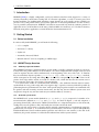
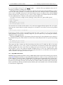
The HORNET NoC system model (defined in sys.hpp and sys.cpp) is composed of a number of interconnected tiles (defined in tile.hpp and tile.cpp). As shown in Figure 1, each tile comprises a
processing element (PE), which can be a MIPS CPU simulator or a script-driven injector or a Pin front-end,
a bridge that converts packets to flits, and, finally, the network switch node itself.
Since each tile can be run in a separate thread, inter-tile communication is synchronized using finegrained locks (see Section 5). To avoid unnecessary synchronization, each tile has a private independently
initialized Mersenne Twister random number generator and collects its own statistics; at the end of the
simulation, the per-tile statistics are collected and combined into whole-system statistics.
1
2
GETTING STARTED
2.2
HORNET Design Overview
Figure 1 A system as simulated by HORNET
sys
tile
pe
pe (cpu or injector)
packet-level I/O
bridge
bridge
dma
· · ·
dma
flit-level I/O
···
node
pe
bridge
node
node
flit-level I/O
(synchronized)
2.2.3
tile
tile_statistics
random_gen
tile_statistics
tile
···
flit-level I/O
(synchronized)
The PE and the bridge
In addition to the base pe class (defined in pe.hpp and pe.cpp), HORNET includes a cycle-level MIPS
CPU simulator with a local memory (cpu.hpp and cpu.cpp), a script-driven injector (injector.hpp
and injector.cpp), and a Pin front-end module. Which mode to use and how to configure them will be
described in detail in Section 3.
The PE interacts with the network via a bridge (bridge.hpp and bridge.cpp), which exposes a
packet-based interface to the PE and a flit-based interface to the network. The bridge exposes a number of
incoming queues which the PE can query and interact with, and provides a number of DMA channels for
sending and receiving packet data. The processing element can check if any incoming queues have waiting
data using bridge::get waiting queues() and query waiting packets with bridge::get queueflow id() and bridge::get queue length(); it can also initiate a packet transfer from one of the
incoming queues with bridge::receive(), start an outgoing packet transfer via bridge::send(),
and check whether the transfer has completed with bridge::get transmission done().
Once the bridge receives a request to send or receive packet data, it claims a free DMA channel (defined
in dma.hpp and dma.cpp) if one is available or reports failure if no channels are free. Each DMA channel
corresponds to a queue inside the network switch node, and slices the packet into flits (flit.hpp and
flit.cpp), appending or stripping a head flit as necessary. The transfer itself is driven by the system
clock in ingress dma channel::tick positive edge() and egress dma channel::tick positive edge().
2.2.4
The network switch node
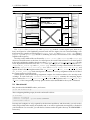
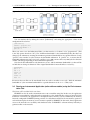
The interconnected switch nodes (see Figure 2) that form the network fabric are responsible for delivering
flits from the source bridge to the destination bridge. The node (defined in node.hpp and node.cpp)
models an ingress-queued wormhole router with highly configurable, table-based route and virtual channel allocation and a configurable crossbar.
2
2
GETTING STARTED
2.3
How to Install
Figure 2 A HORNET network node
node
···
···
channel_alloc
(e.g., set_channel_alloc)
egress
···
···
···
virtual_queue
router
(e.g., set_router)
···
ingress
crossbar
···
egress
···
···
ingress
···
···
···
virtual_queue
The ingress class (ingress.hpp and ingress.cpp) models a router ingress port; there is (at
least) one ingress for each neighboring network node and one ingress for each connected bridge; each
ingress manages a number of virtual queues (virtual_queue.hpp and virtual_queue.cpp). Egresses
(egress.hpp and egress.cpp) contain no buffering and only hold references to the corresponding
neighbor-node ingresses.
Next-hop routes and flow IDs are allocated by router::route() (in router.hpp and router.cpp)
whenever a head flit arrives at the front of a virtual queue; the router holds references to all virtual queues
in the node and directly modifies them by invoking virtual queue::front set next hop(). Specific
router implementations inherit from the router class (for example, the configurable table-driven setrouter in set_router.hpp and set_router.cpp). Similarly, next-hop virtual channel allocation is
handled by channel alloc::allocate() via a call to virtual queue::front set vq id(), and
specific channel allocator implementations like set channel alloc in set_channel_alloc.hpp and
set_channel_alloc.cpp. Each virtual queue remembers its next-hop assignments until the last flit of
the current packet has left the queue.
Virtual queues with valid next-hop assignments compete for crossbar transfers to the next-hop node
or bridge. In each clock cycle, crossbar::tick positive edge() examines the competing ingress
queues and invokes virtual queue::front pop() of the winning queues and virtual queue::back push() of the corresponding next-hop queues until crossbar bandwidth for that cycle is exhausted.
2.3
How to Install
First, download the HORNET archive, and extract:
˜$ tar zxf hornet.tar.gz
After configuring building scripts, do make and install as below:
˜$ cd hornet
˜/hornet$ ./bootstrap
˜/hornet$ ./configure --prefix=$HOME/SOMEWHERE
˜/hornet$ make install
bootstrap and configure are only required for the first time installation, and afterwards, you only need to
make (and possibly make install); the makefiles and so on will be regenerated automagically as needed. If
your installation was successful, you will find two binaries under the prefix directory. If SOMEWHERE =
hornet-inst,
3
2
GETTING STARTED
2.4
Generating a System Image File
˜$ cd hornet-inst
˜/hornet-inst$ cd bin
˜/bin$ ls
darimg darsim
If you see the above two files, you are good to go.
2.4
Generating a System Image File
In order to run a simulation, you first need to write your own configuration file, which basically contains
all the information about network (topology, routing/VC allocation algorithm, queue size, etc.) and in
which mode you are running HORNET (network-only, Pin front-end or MIPS core). We’ll see more details
on how to write the configuration file in Section 3. Once you have your configuration file, say sample.cfg,
darimg is used to generate the system image file from the configuration file, as shown below:
˜/bin$ darimg sample.cfg
This will generate the image file called output.img.
2.5
Running a Simulation
Once the image file is generated, darsim can run a simulation using this system image (output.img) and
various simulation arguments. Below is an example of running a simulation for 1,000,000 cycles using a
network-only mode, where network traffic is fed by ”sample.evt” file (details on the format of an event file
(or network trace) is covered later in Section 3.1.2).
˜/bin$ darsim output.img --events sample.evt --cycles=1000000
Below are the simulation parameters that can be specified (you can also see this information by doing
”darsim -h”):
USAGE: darsim SYSTEM_IMAGE
Options:
--cycles arg
simulate for arg cycles (0 = until drained)
--packets arg
simulate until arg packets arrive (0 = until drained)
--stats-start arg
start statistics after cycle arg (default: 0)
--no-stats
do not report statistics
--no-fast-forward
do not fast-forward when system is drained
--events arg
read event schedule from file arg
--memory-traces arg
read memory traces from file arg
--log-file arg
write a log to file arg
--vcd-file arg
write trace in VCD format to file arg
--vcd-start arg
start VCD dump at time arg (default: 0)
--vcd-end arg
end VCD dump at time arg (default: end of simulation)
--verbosity arg
set console verbosity
--log-verbosity arg
set log verbosity
--random-seed arg
set random seed (default: use system entropy)
--concurrency arg
simulator concurrency (default: automatic)
--sync-period arg
synchronize concurrent simulator every arg cycles (default:
0 = every posedge/negedge)
--tile-mapping arg
specify the tiles-to-threads mapping; arg is one of: ←sequential, round-robin, random (default: random)
--version
show program version and exit
-h [ --help ]
show this help message and exit
Now, let’s see how to configure the system you want to simulate.
4
←-
3
CONFIGURING YOUR SYSTEM
3
Configuring Your System
HORNET can be driven in three different ways: network-only mode, application binary mode (Pin instrumentation tool) and full multicore mode (MIPS core simulator). Depending on your needs, you should choose the
appropriate mode to run HORNET.
3.1
3.1.1
Running a Synthetic Network Traffic using a Trace-driven Injector (Network-Only Mode)
XY Routing on an 8x8 2D Mesh with 2 virtual channels
For the very first example, let’s run the most simplest case: a synthetic benchmark (transpose) on a 2D
8x8 mesh (64 cores) with XY routing. We provide scripts which generate configuration files with typical
settings under scripts/config/ directory. Although you can write your own configuration file from scratch,
it may be easier to start with one of these scripts.
Since we are using DOR routing (XY), we will use dor-o1turn.py. Although the original script generates
multiple configuration files, you can easily change inside the script to only output your target configuration. Below is the part of the script, which is modified to only generate the configuration for XY routing, 2
VCs, dynamic VC allocation on 8 by 8 2D mesh:
...
for dims in [(8,8)]:
for type in [’xy’]:
for oqpf in [False]:
for ofpq in [False]:
xvc=get_xvc_name(oqpf,ofpq)
for nvcs in [2]:
...
dims corresponds to the 8 by 8 mesh, and type corresponds to the routing algorithm, and thus is set to ’xy’.
oqpf and ofpq stand for ”one queue (VC) per flow” and ”one flow per queue”, respectively. These two are
both related to the VC allocation algorithm, and for the conventional, dynamic VC allocation which does
not have any restriction, both are set to ”False”. (For more details on VC allocation, see Section 3.1.5.) nvcs
represents the number of virtual channels per link, and thus set to 2 for our 2-VC setting.
Now with these changes, running the script will give you one configuration file, called ”xy-std-vc2mux1-bw1.cfg”. It looks like below:
[geometry]
height = 8
width = 8
[routing]
node = weighted
queue = set
one queue per flow = false
one flow per queue = false
[node]
queue size = 8
[bandwidth]
cpu = 16/1
net = 16
north = 1/1
east = 1/1
south = 1/1
west = 1/1
[queues]
cpu = 0 1
5
3
CONFIGURING YOUR SYSTEM
3.1
Running a Synthetic Network Traffic using a . . .
net = 8 9
north = 16 18
east = 28 30
south = 20 22
west = 24 26
[core]
default = injector
[flows]
# flow 00 -> 01 using
0x000100@->0x00 = 0,1
0x000100@0x00->0x00 =
0x000100@0x00->0x01 =
# flow 00 -> 02 using
0x000200@->0x00 = 0,1
0x000200@0x00->0x00 =
0x000200@0x00->0x01 =
0x000200@0x01->0x02 =
# flow 00 -> 03 using
... ...
xy routing
0x01@1:24,26
0x01@1:8,9
xy routing
0x01@1:24,26
0x02@1:24,26
0x02@1:8,9
xy routing
The [core] section indicates which core model you are using, and ”injector” means that a trace-driven
injector is being used to drive network traffic (network-only mode). Once you have your configuration file,
let’s generate a system image file as described in Section 2.4.
˜/config$ ˜/hornet-inst/bin/darimg xy-std-vc2-mux1-bw1.cfg
This will generate the system image file, ”output.img”. Now, since we are driving HORNET in a networktrace mode, we need a network trace (or equivalently, an event file).
3.1.2
Trace Format (writing an event file)
The simple trace-driven injector reads a text-format trace of the injection events: each event contains
a timestamp, the flow ID, packet size, and possibly a repeat frequency (for periodic flows). The injector
offers packets to the network at the appropriate times, buffering packets in an injector queue if the network
cannot accept them and attempting retransmission until the packets are injected. When packets reach their
destinations they are immediately discarded.
Below is an example of the injection events:
tick 12094
flow 0x001b0000
tick 12140
flow 0x00001f00
tick 12141
flow 0x001f0000
tick 12212
flow 0x00002100
tick 12212
flow 0x00210000
......
size 13
size 5
size 5
size 5
size 13
The first two lines indicate that at the cycle of 12094, a packet which consists of 13 flits is injected to Node
27 (0x1b), and its destination is Node 0 (0x00). The six low digits of the flow ID 0x001b0000, which is
0x1b0000, are divided into 0x[Src][Dest][00], meaning the source core is 0x1b and the destination core is
0x00. You may need to change this format (especially when you are increasing the number of cores), and
it will work as long as it is consistent with the format used in the [flow] section in the configuration file,
because this flow ID is used to lookup the route information for the specific flow.
Similarly, the next two lines mean that at the cycle of 12140, a 5-flit packet is injected from Node 0,
which is detined to Node 31 (0x1f).
6
3
CONFIGURING YOUR SYSTEM
3.1
Running a Synthetic Network Traffic using a . . .
For periodic events (often used for synthetic benchmarks), on the other hand, we can specify each
injection event as below:
flow 0x010800
flow 0x021000
flow 0x031800
flow 0x042000
flow 0x052800
......
size
size
size
size
size
8
8
8
8
8
period
period
period
period
period
50
50
50
50
50
Note that there is no notion of the absolute time (tick) when the packet is being injected. Instead, by
adding a field named ”period”, you can specify the number of cycles between two subsequent injections
for the same flow. For example, the first line means that the flow 0x010800 (from Node 1 to Node 8) with
the size of 8 flits is being injected to the network every 50 cycles. In this manner, you don’t have to repeat
the injection event, and you can change the amount of traffic by varying this period (smaller the period,
heavier the traffic).
For user’s convenience, we provide a script which generates event files for synthetic benchmarks (bitcomplement, shuffle, transpose, tornado and neighbor) that are often used to evaluate the network performance. The script is called ”synthetic-benchmarks.py” and is located under scripts/event/.
Suppose we want to run Transpose, with the packet size of 8 flits and the period of 50 cycles. In the
script, we need to set parameters as below:
...
for dims in [(8,8)]:
for mode in [’transpose’]:
for size in [8]:
for period in [50]:
...
#network size
#benchmark
#packet size (flits)
#period (cycles)
Running the above script will give you an event file, called ”transpose-s8-p50.evt”.
Since you finally have both the system image and the event file, you can now run the actual simulation
as below:
˜/config$ ˜/hornet-inst/bin/darsim ˜/hornet/scripts/config/output.img --events ˜/ ←hornet/scripts/event/transpose-s8-p50.evt --cycles 100000
3.1.3
Changing Routing Algorithms
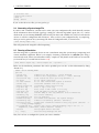
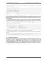
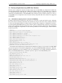
HORNET supports oblivious, static, and adaptive routing. A wide range of oblivious and static routing schemes is possible by configuring per-node routing tables. These are addressed by the flow ID
and the incoming direction {prev node id,flow id}, and each entry is a set of weighted next-hop results
{(next node id,next flow id,weight), ... }. If the set contains more than one next-hop option, one is selected
at random with propensity proportionate to the relevant {weight} field, and the packet is forwarded to
{next node id} with its flow ID renamed to {next flow id}.
7
‐ Per‐node routing table configuration
<prev node id, flow id>
‐ <prev_node_id, flow_id> 3 CONFIGURING YOUR SYSTEM
3.1 Running a Synthetic Network Traffic using a . . .
=> {<next_node_id, next_flow_id, weight>, ...}
Figure 3 Oblivious Routing Algorithms
DA
SA
SB
DOR
V li t
Valiant
ROMM
O1TURN
Let’s take a look at the configuration file how routing is done. There are two sections related to routing:
[routing] and [flows].
[routing]
node = weighted
queue = set
one queue per flow = false
one flow per queue = false
In the ”[routing]” section, the option ”node” specifies how flows determine their next hops. There are two
available values for this: table and weighted. ”Table” is used when you have only one possible next-hop
node, while ”weighted” is used when you can have multiple possible next-hops and choose one among
them according to their weights. Although we provide two options, however, since ”weighted” can support
”table” as well by specifying only one next-hop in the [flows] section, you may fix this value to ”weighted”.
The [flows] section is where all the possible route information is contained. Let’s take a look at the case
of XY routing:
[flows]
# flow 00 -> 01 using
0x000100@->0x00 = 0,1
0x000100@0x00->0x00 =
0x000100@0x00->0x01 =
# flow 00 -> 02 using
0x000200@->0x00 = 0,1
0x000200@0x00->0x00 =
0x000200@0x00->0x01 =
0x000200@0x01->0x02 =
# flow 00 -> 03 using
...
xy routing
0x01@1:24,26
0x01@1:8,9
xy routing
0x01@1:24,26
0x02@1:24,26
0x02@1:8,9
xy routing
In the case of the flow 0x000200, which has the source of Node 0 and the destination of Node 2, the route
using XY routing will be simply Node 0 -¿ Node 1 -¿ Node 2. Basically, the format is as below:
{flow ID}@{prev node}->{current node} = {next node}@{weight}:{virtual channel IDs}
The first line, ”0x000200@-¿0x00 = 0,1”, is the only exception where it does not contain a previous node,
since it indicates the packet injection from Core 0 to Node 0. The availalbe virtual channel IDs for this
path is 0 and 1, as specified in the ”cpu = 0 1” under the [queues] section (see below). The second line,
”0x000200@0x00-¿0x00 = 0x01@1:24,26”, according to the above format, means that the packets of flow
0x000200 that have been injected to Node 0 can proceed to Node 1 via one of the virtual channels (24 or
26). Unique virtual channel IDs are given for all the queues of all the directions, and are specified in the
[queues] section. Here, for example, has 24 and 26, because we have configured each link to have two
virtual channels, and the IDs for the two queues in West-side of the node are 24 and 26. (Caution: the
8
3
CONFIGURING YOUR SYSTEM
3.1
Running a Synthetic Network Traffic using a . . .
direction of the packet is going to East (node 0 -¿ node 1), but you should use the WEST queues of node 1
for this path since the direction represents the position within a node).
[queues]
cpu = 0 1
net = 8 9
north = 16 18
east = 28 30
south = 20 22
west = 24 26
The last line, ”0x000200@0x01-¿0x02 = 0x02@1:8,9”, shows the path from node 2 to core 2, where the packet
is picked up from the network by the destination core. Since the direction is from ”network” to ”cpu”, the
available VC ID’s are 8 and 9, which are specified by ”net = 8 9” above.
Now, how about the case when we have multiple possible paths, say O1TURN? Below is a part of
the routes for O1TURN, showing the routes of the flow from Node 0 to Node 9 (for your information,
the script that generates DOR routes (dor-o1turn.py) can also generate routes for O1TURN by setting the
appropriate value inside the script file) :
# flow 00 -> 09 using
0x000900@->0x00 = 0,1
0x000900@0x00->0x00 =
0x000900@0x00->0x01 =
0x000900@0x01->0x09 =
0x000900@0x00->0x08 =
0x000900@0x08->0x09 =
o1turn routing
0x01@1:24 0x08@1:18
0x09@1:16
0x09@1:8,9
0x09@1:26
0x09@1:8,9
O1TURN gives you two possible routes for the flow from 0 to 9: (Node 0 -¿ Node 1 -¿ Node 9) or (Node
0 -¿ Node 8 -¿ Node 9), whether the packet follows XY or YX, respectively. This can be examined in the
second line of the flow information, which is:
0x000900@0x00->0x00 = 0x01@1:24 0x08@1:18
For the packet at Node 0, which is injected from the core, it has two possible next hops, which are Node 1
and Node 8. Since their weights are both 1, the next hop is picked with an equal probability between the
two. Note that depending on which node is chosen, there can be two different previous nodes at node 9 (1
or 8), and thus, we need to have both routes for 0x000900@0x01-¿0x09 and 0x000900@0x08-¿0x09.
We also provide the script that generates two-phase ROMM and Valiant, called romm2-valiant.py.
To use adaptive routing, all allowed next hops must first be specified in the HORNET’s flows section
in the format described above. Among the possible next hops, one node will be chosen depending on
the multi-path routing setup in the HORNET configuration file. You have three different choices for the
adaptive algorithm, and can specify which one to use by adding the key called ”multi-path routing” in the
”[routing]” section as below:
[routing]
multi-path routing = adaptive_queue
Three different values for the ”multi-path routing” option are:
• probability
- (default) If there are multiple neighbor nodes that a packet may take as the next hop at the current
node, one node is randomly chosen according to the specified probability ratio between those nodes.
Randomized oblivious routing schemes such as O1TURN, ROMM or Valiant can be used with this
configuration.
• adaptive queue
- Among the next hop candidates, the one which has the largest number of available virtual channels
for the packet being routed will be chosen. The probability scheme is used as a tie breaker.
9
3
CONFIGURING YOUR SYSTEM
3.1
Running a Synthetic Network Traffic using a . . .
VC Buffer Configurations
g
• adaptive packet
- Among the next hop candidates, the one to which the least number of other packets at the current
node are routed will be chosen. The probability scheme is used as a tie breaker.
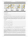
3.1.4
Changing the Number of Virtual Channels
Figure 4 Virtual Channel Configurations
CPU
net
N
W
E
S
We can easily change the number of virtual channels in the [queues] section of the configuration file. As
in the figure, each node basically has six different directions, and we can configure each link separately as
below in the case of 2 virtual channels for all links:
[queues]
cpu = 0 1
net = 8 9
north = 16 18
east = 28 30
south = 20 22
west = 24 26
## of VCs, VC buffer size are con
of VCs VC buffer size are con
Each port can have different co
Although there is no problem as long as VC ID’s are unique, one thing you need to be careful is that they
should match with the queues you used to specify the routes in ”[flows]” section. Here is another example
when there are 4 VCs within the network and 8 VCs between cpu and node:
[queues]
cpu = 0 1 2 3 4 5 6 7
net = 8 9 10 11 12 13 14 15
north = 16 17 18 19
east = 40 41 42 43
south = 24 25 26 27
west = 32 33 34 35
3.1.5
Changing Virtual Channel Allocation Schemes
Like routing, virtual channel allocation (VCA) is table-driven. The VCA table lookup uses the nexthop node and flow ID computed in the route computation step, and is addressed by the four-tuple
{prev node id,flow id,next node id,next flow id}. As with table-driven routing, each lookup may result
10
3
CONFIGURING YOUR SYSTEM
3.1
Running a Synthetic Network Traffic using a . . .
in a set of possible next-hop VCs {(next vc id,weight), ... }, and the VCA step randomly selects one VC
among the possibilities according to the weights.
This directly supports dynamic VCA (all VCs are listed in the result with equal probabilities) as well as
static VCA (the VC is a function of on the flow ID). Most other VCA schemes are used to avoid deadlock,
such as that of O1TURN (where the XY and YX subroutes must be on different VCs), Valiant/ROMM
(where each phase has a separate VC set), as well as various adaptive VCA schemes like the turn model,
are easily implemented as a function of the current and next-hop flow IDs.
Let’s take a look at the example. In the ”[routing]” section, there is an option called ”queue”.
[routing]
node = weighted
queue = set
one queue per flow = false
one flow per queue = false
As was for the case of ”node”, fix this value to ”set”, since it can support all other options. The ”set” option
means that the virtual channel is picked among the set of listed VCs in the flows section with specified
weights.
0x000100@0x00->0x01 = 0x01@1:8,9
For the above, when the packet is forwarded from node 0 to node 1, either VC 8 or 9 is chosen with the
equal probability. If you want to statically assign VCs, you can achieve it by only listing the statically
assigned VC for the specific flow.
Separately, HORNET supports VCA schemes where the next-hop VC choice depends on the contents of
the possible next-hop VCs, such as EDVCA or FAA. This is achieved by the below two options in [routing]
section:
one queue per flow = false
one flow per queue = false
”One queue per flow” restricts any flow from using more than one VC within any link at any given
snapshot. When this is set to ”true”, packets are guaranteed to be delivered in-order under single-path
routing algorithms since there exists only one unique path across the network at any given time. ”One
flow per queue”, if set to true, limits the number of distinct flows to one for any virtual channel within
a link. This means that if a specific VC contains any packet from flow A, no other flows can use that VC
until it is drained to be empty, even there is a space.
3.1.6
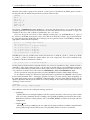
Using Bidirectional Links
HORNET supports bidirectional links, namely a Bandwidth-Adaptive Network (for details, please read the
paper [BAN]). Bidirectional links can optionally change direction as often as on every cycle based on local
traffic conditions, effectively trading off bandwidth in one direction for bandwidth in the opposite direction. To achieve this, each link is associated with a modeled hardware arbiter which collects information
from the two ports facing each other across the link (for example, number of packets ready to traverse the
link in each direction and the available destination buffer space) and suitably sets the allowed bandwidth
in each direction. (Figure XXX).
11
3
• DARSIM supports bidirectional links.
DARSIM supports bidirectional links
CONFIGURING YOUR SYSTEM
3.2 Running an Instrumented Application (native . . .
‐ Runtime Arbitration of the direction of links based on the amount of traffic that needs to be transferred.
Figure 5 Bandwidth Adaptive Network
can simulate this by adding the section ”[arbitration]” and setting the appropriate values in the
‐ You
“Oblivious Routing in On‐Chip Bandwidth‐Adaptive Networks” [Cho et al./PACT’09]
configuration file as below:
[arbitration]
scheme = proportional
minimum bandwidth = 1
period = 1
When you want to use the bidirectional links, you first need to set ”scheme” to be ”proportional”. (This
is the only option other than ”off”). The ”minimum bandwidth” is the bandwidth (in flits) that does not
change by the arbitration, meaning the minimum guaranteed bandwidth in any specific direction. Lastly,
”period” is the number of cycles between the bandwidth arbitration. If ”period” is 1, it means that the
bandwidth arbitration is done every cycle, and if it is set to 100, it means that every 100 cycles the direction
of links will change depending on the bandwidth requirement.
Note that if the bandwidth for each direction is set to 1 and the minimum bandwidth is 1, there will be
no link that can change its direction. If the original bandwidth for network links is 2 as below,:
[bandwidth]
cpu = 8
net = 8
north = 2
east = 2
south = 2
west = 2
this means that two flits can be transferred from one node to another at one cycle. With the minimum
bandwidth of 1, the maximum bandwidth for a specific direction can be 2 + 1 = 3 flits/cycle.
3.2
Running an Instrumented Application (native x86 executables) using the Pin Instrumentation Tool
This feature will be included in the next release..
HORNET can also be used to instrument native x86 executables using Pin. In this case, the application
of interest is run under Pin, and its threads are mapped 1:1 to the simulated tiles as they are spawned. Each
instruction executed by the application is intercepted and its memory accesses handled by the memory
hierarchy configured in HORNET; timing consists of a table-driven model for the non-memory portion of
each instruction plus the memory access latencies reported by HORNET. In this mode, direct application
access to the network is not available, and simulation relies on HORNET’s coherent memory hierarchy to
generate traffic on the network.
12
3
CONFIGURING YOUR SYSTEM
3.3
3.3
Running an Application using a MIPS Core . . .
Running an Application using a MIPS Core Simulator
Each tile can be configured to simulate a built-in single-cycle in-order MIPS core, which can be loaded with
statically linked binaries compiled with a MIPS cross-compiler such as GCC. The MIPS core is connected
to a memory hierarchy which consists of a local L1/L2 cache. Memory coherence among the caches is
ensured by an implementation of the MSI/MESI cache coherence protocol. Before moving on to how to
use the MIPS core, it is important to know how the memory subsystem and cache coherence are supported
by HORNET.
3.3.1
Shared Memory Support (private-L1 and shared-L2 MSI/MESI)
In Hornet shared memory framework, each tile has its own local L1 cache and local L2 cache. Although
these local caches are directly connected to the attached core only, L1 and/or L2 caches could be connected
to other cores through the Hornet on-chip network. Our first release supports a configuration of privateL1 and shared-L2 MSI/MESI memory, where both L1 and L2 (combined with a directory) can send and
receive cache coherence messages to/from any cores. The type of memory subsystem is also specified in
the Hornet configuration script. Below are all common parameters of all memory types, which is defined
in [memory] section.
[memory]
architecture = private-shared MSI/MESI
dram controller location = top and bottom
core address translation = stripe
core address translation latency = 1
core address translation allocation unit in bytes = 4096
core address synch delay = 0
core address number of ports = 0
dram controller latency = 2
one-way offchip latency = 150
dram latency = 50
dram message header size in words = 4
maximum requests in flight per dram controller = 256
bandwidth in words per dram controller = 4
The first line tells which memory architecture the simulation is going to use. In order to use MSI/MESI
protocol with private-L1 shared-L2 configuration, use private-shared MSI/MESI architecture. Memoryspecific configurations are given similarly to the core configurations. For example, detailed parameters of
private-shared MSI/MESI memory is defined in [memory::private-shared MSI/MESI] section.
[memory::private-shared MSI/MESI]
use Exclusive state = no
words per cache line = 8
memory access ports for local core = 2
L1 work table size = 4
shared L2 work table size = 4
reserved L2 work table size for cache replies = 1
reserved L2 work table size for line eviction = 1
total lines in L1 = 256
associativity in L1 = 2
hit test latency in L1 = 2
read ports in L1 = 2
write ports in L1 = 1
replacement policy in L1 = LRU
total lines in L2 = 4096
associativity in L2 = 4
hit test latency in L2 = 4
read ports in L2 = 2
write ports in L2 = 1
replacement policy in L2 = LRU
13
3
CONFIGURING YOUR SYSTEM
3.3.2
3.3
Running an Application using a MIPS Core . . .
Network configuration
Network is configured in the same way how original Hornet simulator is configured. However, the network
must provide enough number of disjoint virtual channel sets to support the total number of message
channels that core and memory models need to use. The best practice is to have different flow IDs for
different message channels by adding prefix to it. Configure your Hornet routing configuration in such a
way that the flows with the same prefix in their flow IDs will use the same virtual channel set. To make
your life easier, dar/scripts/config/xy-shmem.py script helps creating the routing configuration with the
following parameters.
-x
-y
-v
-q
-c
-m
-n
-o
(arg)
(arg)
(arg)
(arg)
(arg)
(arg)
(arg)
(arg)
:
:
:
:
:
:
:
:
network width (8)
network height (8)
number of virtual channels per set (1)
capacity of each virtual channel in flits(4)
core type (memtraceCore)
memory type (privateSharedMSI)
number of VC sets
output filename (output.cfg)
This script will generate routing configurations as well as the list of default parameters of given
core/memory types. Make sure the -n option specifies no less than the total number of message channels being used by the core and memory model.
3.3.3
Running an application
Now, with the shared memory configured, let’s move on to the MIPS core. An example application
(blackscholes stock option valuation) running on MIPS cores is given in /examples/blackscholes. In
general: in order to run a MIPS core simulation, you must add:
• --enable-mips-rts flag to the ./configure (which is discussed in Section 2.3).
• The following lines to your application’s configuration (*.cfg) file:
[core]
default = mcpu
[code]
default = X.mips
”mcpu” stands for MIPS cpu and ”X.mips” corresponds to the object file output by the MIPS crosscompiler. Aside: Two additional sections needed to run MIPS simulations are ”[instruction memory hierarchy]” and ”[memory hierarchy]”---users need not specify these sections (with a default configuration
of local L1 and L2 caches per core), however, as they are automatically generated by ”xy-shmem.py”. A
makefile designed to compile and run a MIPS core simulation is given in /examples/blackscholes.
(This makefile assumes that you are using a cross-compiler called linux-gnu-gcc and mips-linux-gnu-ld
cross-compilers.)
MIPS core based simulations assume that every core will be running the same thread code. If master/worker thread style computation is needed, the union of the master/thread code must be included in
a single source file. Choosing which core is home to a master or worker thread at runtime can be made
through a system call that checks thread ID.
More generally, the system call API (API descriptions are given in /src/rts/rts.h.) is accessible
if #include"rts.h" is included. At a high level, the system call API provides the following classes of
functionality:
• [Hardware] Poll the processor for various quantities such as CPU id, current thread ID, cycle count,
and similar.
• [Memory Hierarchy] Enable/disable magic single-cycle memory operations, perform un-cached loads
and stores. Un-cached loads and stores can be used to implement barriers.
14
4
STATISTICS
• [Printers] Print and flush various types (int, string, etc) to the console.
• [Intrinsics] Perform function intrinsics (log, sqrt, ...).
• [File I/O] Open a file, read lines into simulator memory, close file operations.
• [Network] Send/receive on specific flows and poll for packets in specific queues. All flow processes
are DMA, freeing the MIPS core while the packets are being sent/received.
• [Dynamic Memory Management] Malloc and friends. Note that when using malloc, if threads, other
than the thread that made the malloc call, refer to the memory allocated by the malloc, a static address
that points to the malloced memory must be made and used by those other threads. This workaround
is exemplified in the blackscholes example through the double pointers whose names are prefixed
by __PROXY_.
3.3.4
Troubleshooting
If when running a MIPS core simulation you see an error labeled:
terminate called after throwing an instance of ‘err_tbd’
your cross-compiler has emitted an instruction that was not implemented by Hornet. To get around this
problem you have two options:
• In /src/exec/mcpu.cpp, implement the unimplemented instruction.
• Try to find a cross-compiler capable of emitting supported instructions (one that is known to work is
mips-linux-gnu-gcc(SourceryG++Lite4.4-303)4.4.1).
4
Statistics
HORNET collects various statistics during the simulation. To avoid synchronization in a multi-threaded
simulation, each tile collects its own statistics (class tile statistics in statistics.hpp and statistics.
cpp); a system statistics object keeps track of the tile statistics objects and combines them to
report whole-system statistics at the end of the simulation.
To accurately collect per-flit statistics when the simulation threads are only loosely barrier-synchronized,
some counters (for example, the elapsed flit transit time) are stored and carried together with the flit (see
flit.hpp), and updated during every clock cycle.
After your simulation has completed, you will see many statistics being printed out on the screen (you
can redirect the output to a file). Below is the part of the output, which shows throughput and latency for
each flow, and the entire average of all flows.
flit counts:
flow 00010000: offered 58, sent 58, received 58 (0 in flight)
flow 00020000: offered 44, sent 44, received 44 (0 in flight)
flow 00030000: offered 34, sent 34, received 34 (0 in flight)
flow 00040700: offered 32, sent 32, received 32 (0 in flight)
flow 00050700: offered 34, sent 34, received 34 (0 in flight)
.....
all flows counts: offered 109724, sent 109724, received 109724 (0 in flight)
in-network sent flit latencies (mean +/- s.d., [min..max] in # cycles):
flow 00010000: 4.06897 +/- 0.364931, range [4..6]
flow 00020000: 5.20455 +/- 0.756173, range [5..9]
flow 00030000: 6.38235 +/- 0.874969, range [6..10]
flow 00040700: 6.1875 +/- 0.526634, range [6..8]
flow 00050700: 5.11765 +/- 0.32219, range [5..6]
.....
all flows in-network flit latency: 9.95079 +/- 20.5398
15
5
SPEEDING UP YOUR SIMULATION . . .
Basically, statistics are collected for the entire simulation period unless you specify the command line
option, ”--stats-start”. If you specify the option with, say N cycles, however, you need to be careful how
the statistics are collected. Since each packet is made to be responsible for its own statistics in order to
achieve synchronized parallel simulation (packet carries its own timestamp around), statistics are measured
at the packet granularity. In other words, when each packet is FIRST generated and sits inside the buffer
(assumed to be infinite) waiting to be injected to the network, it is assigned its timestamp of ”birth”. By
saying that we will collect data starting from cycle N, packets whose birth timestamps are greater than N
are only considered. This means that if we set a comparably large N under very high traffic, so that many
packets born before cycle N are still waiting to be injected to the network, they will NOT be included in
the statistics even if they are actually injected to and drained from the network after cycle N.
5
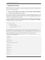
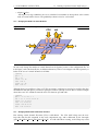
Speeding Up Your Simulation (Parallel Simulation)
Figure 6 Parallelization speedup for cycle-accurate, 1024-core simulations
speedup vs. single thread
13×
11×
9×
7×
5×
3×
1×
1
2
3
4
5
6
synthetic, cycle-accurate
7
8
9
10
11
12 13 14 15 16 17 18 19 20 21 22 23
# simulation threads (each pinned to a separate HT core)
synthetic, 5-cycle sync
blackscholes, cycle-accurate
blackscholes, 5-cycle sync
24
HORNET takes advantage of modern multicore processors by automatically distributing simulation work
among the available cores, resulting in speedup of the simulations. The simulated system is divided into
tiles comprising a single virtual channel router and any traffic generators connected to it, as well as a
private pseudorandom number generator and any data structures required for collecting statistics. One
execution thread is spawned for each available processor core (and restricted to run only on that core), and
each tile is mapped to a thread; thus, some threads may be responsible for multiple tiles but a tile is never
split across threads. Inter-thread communication is thus limited to flits crossing from one node to another,
and some fundamentally sequential but rarely used features (such as writing VCD dumps).
Functional correctness requires that inter-tile communication be safe: that is, that all flits in transit
across a tile-to-tile link arrive in the order they were sent, and that any metadata kept by the virtual
channel buffers (e.g., the number of flits remaining in the packet at the head of the buffer) is correctly
updated. In multithreaded simulation mode, HORNET accomplishes this by adding two fine-grained
locks in each virtual channel buffer---one lock at the tail (ingress) end of the VC buffer and one lock at the
head (egress) end---thus permitting concurrent access to each buffer by the two communicating threads.
Because the VC buffer queues are the only point of communication between the two threads, correctly
locking the ends when updates are made ensures that no data is lost or reordered.
The virtual queue (defined in virtual_queue.hpp and virtual_queue.cpp) models a virtual
channel buffer, and, as the only point of inter-thread communication, is synchronized in multi-thread
simulations. The fine-grained synchronization ensures correctness even if the simulation threads are only
loosely synchronized.
Synchronization is achieved via two mutual exclusion locks: virtual queue::front mutex and
virtual queue::back mutex. During a positive edge of the clock, the two ends of the queue are
independent, and operations on the front of the queue (e.g., virtual queue::front pop()) only lock
16
REFERENCES
front mutex while operations on the back (e.g., virtual queue::back push()) only lock back mutex; because no communication between the two occurs, flits added to the back of the queue are not
observed at the front of the queue in the same cycle (so, for example, virtual queue::back is full() can report a full queue even if a flit was removed via virtual queue::front pop() during
the same positive edge. During the negative clock edge, the changes made during the positive edge are
communicated between the two ends of the queue, and both locks are held.
With functional correctness ensured, we can focus on the correctness of the performance model. One
aspect of this is the faithful modeling of the parallelism inherent in synchronous hardware, and applies
even for single-threaded simulation; HORNET handles this by having a positive-edge stage (when computations and writes occur, but are not visible when read) and a separate negative-edge stage (when the
written data are made visible) for every clock cycle.
Another aspect arises in concurrent simulation: a simulated tile may instantaneously (in one clock
cycle) observe a set of changes effected by another tile over several clock cycles. A clock-cycle counter
is a simple example of this; other effects may include observing the effects of too many (or too few) flit
arrivals and different relative flit arrivals. A significant portion of these effects is addressed by keeping
most collected statistics with the flits being transferred and updating them on the fly; for example, a
flit’s latency is updated incrementally at each node as the flit makes progress through the system, and
is therefore immune to variation in the relative clock rates of different tiles. The remaining inaccuracy is
controlled by periodically synchronizing all threads on a barrier. 100% accuracy demands that threads be
synchronized twice per clock cycle (once on the positive edge and once on the negative edge), and, indeed,
simulation results in that mode precisely match those obtained from sequential simulation. Less frequent
synchronizations are also possible, which result in significant speed benefits at the cost of minor accuracy
loss.
Below are the command line options, which control the number of concurrent threads, the synchronization period between those threads, and how to distribute the target tiles to the simulating threads.
--concurrency arg
simulator concurrency (default: automatic)
--sync-period arg
synchronize concurrent simulator every arg cycles (default:
0 = every posedge/negedge)
--tile-mapping arg
specify the tiles-to-threads mapping; arg is one of: ←sequential, round-robin, random (default: random)
6
←-
References
[HOR]
Mieszko Lis, Pengju Ren, Myong Hyon Cho, Keun Sup Shim, Christopher W. Fletcher,
Omer Khan and Srinivas Devadas (2011). Scalable, Accurate Multicore Simulation in the
1000-core era. in Proceedings of ISPASS 2011.
[BAN]
Myong Hyon Cho, Mieszko Lis, Keun Sup Shim, Michel Kinsy, Tina Wen and Srinivas
Devadas (2009). Oblivious Routing in On-Chip Bandwidth-Adaptive Networks. in Proceedings of PACT 2009.
17