Download "user manual"

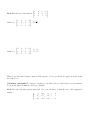
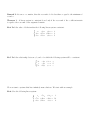
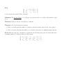
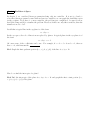
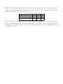
Sec 2.1 Row Operations and Gaussian Elimination
Consider a system of linear equations


x1 −2x2
2x2

−4x1 +5x2

1 −2
2
The coefficient matrix of the system is  0
−4
5

1 −2

The augmented matrix of the system is 
2
 0
−4
5
+x3 =
0
−8x3 =
8
+9x3 = −9

1
−8 .
9

.
1 ..
0

.
−8 ..
8 
.
.
9 .. −9
Note that the number of columns of the coefficient matrix of a given system equals the number
in that system.
of
Remark Given a matrix A, we can construct a linear system having
A as the augmented ma
2 3 1
trix. For example, the linear system we can recover from a matrix
is
−1 0 7
We are mainly interested in solving a given system, i.e., finding the solution set of the system. We
will develop several methods to do so.
Ex.1 Consider systems

x1 −2x2 +x3 =
0

2x2 −8x3 =
8
I.

−4x1 +5x2 +9x3 = −9
and

7
 x1 −2x2 −x3 =
x2 −2x3 = −10 .
II.

x3 =
4
System II is easier to solve; indeed we can solve II using backward substitution.
One idea to solve a general (more complicated) system such as I is to change it to a “triangular”
system like II. When we change the original system, we should be careful not to change the solution
set of the system. But How?
Fact 1 (scaling operation) If we replace an equation in a linear system by a nonzero multiple
of the equation, the solution set remains unchanged.
Ex.2 Let


2x1 −4x2 +2x3 =
0
0
2x2 −8x3 =
8
I.

−4x1 +5x2 +9x3 = −9
and


x1 −2x2 +x3 =
0
x2 −4x3 =
4 ,
I .

−4x1 +5x2 +9x3 = −9
00
then both I0 and I00 are equivalent to I. In other words, systems I, I0 , and I00 are essentially the same.
Notation:
Fact 2 (interchange operation) If we interchange two equations in a system, the solution set
remains unchanged.
Ex.3 Consider


x1 −2x2 +x3 =
0
I . −4x1 +5x2 +9x3 = −9 ,

2x2 −8x3 =
8
000
then I000 is equivalent to I.
Notation:
Fact 3 (replacement operation) If we replace one equation in a system by the sum of itself
and a multiple of another equation, the solution set remains unchanged.
Ex.4 The system

+x3 =
0
 x1 −2x2
2x2 −8x3 =
8
I(iv) .

−3x2 +13x3 = −9
is obtained by replacing
Notation:
of system I by
of I.
Definition Three operations described above are called elementary row operations. Thus elementary row operations do NOT alter the solution set of the original system.
So, how to change a general

x1 −2x2

2x2

−4x1 +5x2

 x1
−−−−−−−−→

system to a triangular one? Let’s take system I as an example.

+x3 =
0
+x3 =
0
 x1 −2x2
−8x3 =
8 −−−−−−−−→
2x2 −8x3 =
8

+9x3 = −9
−3x2 +13x3 = −9

−2x2
+x3 =
0
 x1 −2x2 +x3 = 0
x2 −4x3 =
4 −−−−−−−−→
x2 −4x3 = 4 .

−3x2 +13x3 = −9
x3 = 3
It is easy to find the solution to the last system: x3 =
, x2 =
, x1 =
Now let’s describe the process above in terms of the augmented matrices:



..
.
1 −2
1 .
0
1 −2
1 ..
0



..
.
 0


2 −8 .
8  −−−−−−−−→  0
2 −8 ..
8

..
..
−4
5
9 . −9
0 −3 13 . −9


−−−−−−−−→ 

..
.
..
.
..
.




 −−−−−−−−→ 


..
.
..
.
..
.
.






.

From the last matrix, we recover a system

 x1 −2x2 +x3 = 0
x2 −4x3 = 4

x3 = 3
and the solution of this new system is exactly the same as what we met before.
Remark This method is called the Gauss-Jordan elimination.
Definition Two matrices are row equivalent if there is a sequence of elementary row operations
that transforms one matrix into the other.
Ex.5 Solve the system
III.


x2 −4x3 = 8
2x1 −3x2 +2x3 = 1 .

5x1 −8x2 +7x3 = 1

..
0
1 −4 . 8


.
 2 −3
2 .. 1 

 −−−−−−−−→
.
5 −8
7 .. 1

From the last matrix, we recover a system
Therefore, system III is
.
From the experience above, we know that “triangular” or “steplike” matrices are good, because
the systems associated with such matrices are then easy to solve. We want to define these nice
matrices rigorously.
Definition A matrix is said to be in echelon form (or row echelon form) if it has the following
four properties:
1.
2.
3.
4.
The leftmost nonzero entry in each row is a 1 (called leading 1),
The entries below any leading 1 are all 0,
The leading 1 for each row is to the left of the leading 1 for any row below it,
Any row of all zeros is located below the rows that have leading 1s.


1 4
0 1
Ex.6  0 1 −1 3  is NOT in echelon form. It violates condition 2.
0 1 −3 0


0 1 2 0
. If we switch rows 1
Ex.7  1 2 3 0  is NOT in echelon form. It violates condition
0 0 0 0
and 2, then it will be in echelon form.


1 2 0 0
Ex.8  0 0 0 0  is NOT in echelon form. It violates condition
. If we switch rows 2
0 0 1 0
and 3, then it will be in echelon form.


1 2 3 4
 0 1 1 1 

Ex.9 
 0 0 0 1  is in echelon form.
0 0 0 0
Roughly speaking, matrices in echelon form look like (∗ indicates



1 ∗ ∗ ∗
1 ∗ ∗ ∗
 0 0 1 ∗
 0 1 ∗ ∗  or 
 0 0 0 1
0 0 1 ∗
0 0 0 0
that any number can be present)

∗
∗ 

∗ 
0
As mentioned before, the significance of row echelon form is that when the augmented matrix of a
system is reduced to this form via row operations, the solution of the system is easily obtained by
backward substitution.
Remark There is one flaw in row echelon forms: a row echelon form of a matrix is not unique.
In other words, if two people start with a given matrix and perform different sequences of row operations until a row echelon form is obtained, their final matrices may not be identical. To resolve this
problem, we consider reduced row echelon form.
Sec 2.2 Reduced Echelon Form
Let’s go back to system I in Ex.1 in the previous section. The augmented matrix associated with
system I is


.
1 −2
1 ..
0


..

 0
2
−8
.
8


..
−4
5
9 . −9
which after some row operations becomes

.
1 −2
1 .. 0

.
 0
1 −4 .. 4

.
0
0
1 .. 3


.
1 .. 0
 R1 7→R1 +2R2
.
1 −4 .. 4 
 −−−−−−−→
..
0
1 . 3
1 −2

 0

0


.


.
1 0 −7 .. 8


7→R1 +7R3
 0 1 −4 ... 4  −R−1−
−−−→

 R2 7→−
R2 +4R3
..
0 0
1 . 3


.
1 0 0 .. 29


 0 1 0 ... 16 .


..
0 0 1 . 3

The system we get from the last matrix is
and we immediately get a (unique) solution x1
need backward substitution is that the matrix

1
 0
0
= 29, x2 = 16, and x3 = 3. The reason we do not

0 0
1 0 
0 1
is even nicer than echelon matrices. To be more precise, we need a definition.
Definition Recall that a matrix is said to be in echelon form if it has the following four properties:
1.
2.
3.
4.
The leftmost nonzero entry in each row is a 1 (called leading 1),
The entries below any leading 1 are all 0,
The leading 1 for each row is to the left of the leading 1 for any row below it,
Any row of all zeros is located below the rows that have leading 1s.
If a matrix in echelon form satisfies the following additional condition, then it is said to be in
reduced echelon form (or reduced row echelon form):
5. All entries above any leading 1 are zero. In other words, each leading 1 is the only nonzero
number in its column.


1 2 3 4
 0 1 1 1 

Ex.1 
 0 0 0 1  is in echelon form, but NOT in reduced echelon form, because it violates
0 0 0 0
.
condition


1 0 0 0
 0 1 1 0 

Ex.2 
 0 0 0 1  is in reduced echelon form.
0 0 0 0

1
 0
Ex.3 How about 
 0
0
0
1
0
0
3
1
0
0

0
0 
?
1 
0
Roughly speaking, matrices in echelon form look like (∗ indicates



1 ∗ 0 0
1 0 0 ∗
 0 0 1 0
 0 1 0 ∗  or 
 0 0 0 1
0 0 1 ∗
0 0 0 0
Ex.4 Put

1 −2
 0
1
0
0
that any number can be present)

∗
∗ 

∗ 
0
the following matrix in reduced echelon form:

4
5 −3
3 −1
7 
0
1
2
Why do people like reduced echelon forms more than echelon forms?
Theorem The reduced row echelon form (rref) associated with a matrix is uniquely determined.


2
4
6 −2
0 −3
1 .
Ex.8 Find the rref of the matrix  1
1 −1
3
0


2
4
6 −2
R1 7→ 1 R1
0 −3
1  −−−−2−→
Method 1:  1
1 −1
3
0


2
4
6 −2
R ←→R2
0 −3
1  −−1−−−→
Method 2:  1
1 −1
3
0
Thus we get the same result no matter what sequence of row operations we apply, as stated in the
theorem above.
Calculator commands We can use a calculator to find the reduced echelon form of a given matrix.
Look up the function rref in your User’s Manual.
Ex.9 Solve the following system using rref. Use your calculator to find the rref of the augmented
matrix.

x1 +2x2 +x3 =
4

3x1 +7x2 −2x3 =
1

−2x1 +3x2 +3x3 = −1
Ex.10 Solve the following system using calculator.

x2 −4x3 = 8

2x1 −3x2 +2x3 = 1 .

5x1 −8x2 +7x3 = 1
How should we interpret the result?
Ex.11 Solve the two systems

x1 +2x2 −x3 =
4

3x1 +7x2 −2x3 =
1

−2x1 +3x2 +3x3 = −1
and


x1 +2x2 −x3 = −2
3x1 +7x2 −2x3 =
5

−2x1 +3x2 +3x3 =
3
Sec 2.3 Consistency and Row Rank
Recall that a system of linear equations is said to be consistent if it has one or infinitely many
solutions. A linear system is said to be inconsistent if it has no solutions.
Ex.1 Show that the following system is inconsistent.

1 3 −1
1

 1 4
2 −2

2 7
1 −1

..
. 1

..
. 3 

..
. 6
The reason the above system is inconsistent is that the bottom row of the rref is of the form
.
[ 0 0 0 0 .. 1 ],
which would mean that the corresponding equation is
0 = 1.
This observation gives a simple but nice criterion for consistency of systems.
Definition The row rank of a matrix is the number of nonzero rows in a (reduced) row echelon
form of the matrix.
Ex.2 Determine the row rank of each of the following matrices:




1 3 −1
1 1
1 2 1 2
 1 4
 1 2 0 3 
2 −2 3 
2 7
1 −1 6
2 4 1 5


4
2 −7
 0
0
2 
0 −2
5
Ex.3 Given a linear system, the row rank of the coefficient matrix is always
the row rank of the augmented matrix.
Remark If A is an m × n matrix, then the row rank of A is less than or equal to the minimum of
m and n.
Theorem 1. A linear system is consistent if and only if the row rank of the coefficient matrix
is equal to the row rank of the augmented matrix.
Ex.4 Find the value of k that makes the following linear system consistent:

 x1 −6x2 +2x3 = 8
4x1 −25x2 +10x3 = 6

2x1 −13x2 +6x3 = k
Ex.5 Find the relationship between a, b, and c for which the following system will be consistent:

 3x −9y +3z = a
x −2y −z = b

5x −13y +z = c
We now turn to systems that have infinitely man solutions. We start with an example.
Ex.6 Solve the following linear system:

x1 −5x2 +2x3 = 3

−7x1 +43x2 −30x3 = 19

−2x1 +12x2 −8x3 = 4
In general, how to represent the solution set when there are infinitely many solutions? One way to
do this is parametric representation. The procedure can be described as follows:
Step 1:
Step 2:
Step 3:
Step 4:
Ex.7 Solve the following linear system:
x1 +3x2 +4x3 −2x4 = 3
2x1 +6x2 +9x3 −3x4 = 8
Ex.8 A dairy company makes breakfast, lunch, and dinner meals from a mixture of curds and whey.
The breakfast uses 10 ounces of curds and 40 ounces of whey per batch. The lunch uses 20 ounces of
curds and 90 ounces of whey per batch. The dinner uses 30 ounces of curds and 30 ounces of whey
per batch. There are 300 ounces of curds and 500 ounces of whey on hand. Find the number (must
be an integer) of batches that will use the entire supply.
Definition A linear system is called homogeneous if all of the constant terms are 0.
Ex.9


x1 +3x2 +4x3 = 0
2x1 −x2 +9x3 = 0

−2x1 −x2 +x3 = 0
is a homogeneous system. Is this consistent?
Definition The trivial solution to a homogeneous system is the zero solution (all variables equal
zero).
Theorem 2. Every homogeneous system is consistent.
Theorem 3. For any homogeneous system,
a. If the row rank equals the number of variables, then the trivial solution is the only solution.
b. If the row rank is less than the number of of variables, then there are infinitely many solutions.
Ex.10 Without doing any computation, explain why the following homogeneous system must have
an infinite number of solutions; then solve the system.

 −3x1 +6x2 −x3 +x4 −7x5 = 0
x1 −2x2 +2x3 +3x4 −x5 = 0

2x1 −4x2 +5x3 +8x4 −4x5 = 0
Sec 2.4 Euclidean 3-Space
In chapter 1, we considered linear programs involving only two variables. It is not too hard to
solve these linear programs because when we have two variables, we can graph the feasibility region
in the xy-plane. If we have 3 or more variables, the problem gets complicated, because it is now
hard (if not impossible) to visualize the problem. However, if there are only three variables, then the
situation is not too bad.
Recall that a typical line in the xy-plane is of the form
ax + by = c.
In the xyz-space, the role of lines is now replaced by planes. A typical plane in the xyz-plane is of
the form
ax + by + cz = d.
Of course some of the coefficients can be zero. For example, if a = b = d = 0 and c = 1, then we
.
have z = 0, which means the
Ex.1 Graph the first quadrant portion (i.e., x ≥ 0, y ≥ 0) of the line 2x + 3y = 12.
How do we find the intercepts of a plane?
Ex.2 Find the intercepts of the plane 4x + 8y + 2z = 16 and graph the first octant portion (i.e.,
x ≥ 0, y ≥ 0, z ≥ 0) of the plane.
Definition The equation of a plane written in the form
x
y
z
+ + =1
A B C
is called the intercept form.
Ex.3 Find the intercept form of planes 3x + 4y + 24z = 12 and 3x + 5y + 8z = 6. Sketch the
first octant portion of these planes.
Not every plane has the intercept form.
Ex.4 Sketch the first octant portion of the plane 5x + 3y − 3z = 0.
Going back to the two dimensional case, let’s consider the interaction of two lines in the xy-plane.
Ex.5 Solve each of the following systems by graphing them.
x +2y = 4
x −2y = 6
I.
II.
2x −y = 18
2x −4y = 5
III.
x −2y = 6
2x −4y = 12
Now we consider the interaction of two planes.
Ex.6 Solve each of the following systems.
x +y +z = 1
x +y +z = 1
IV.
V.
x −y +z = 3
x +y +z = 3
VI.
x +y +z = 1
2x +2y +2z = 2
From the example above, we see that the following is generally true.
Theorem Two planes are either identical or parallel if and only if the x, y, z coefficients of one
plane are common multiples, respectively, of the x, y, z coefficients of the other plane.
The interaction of three planes is much more complicated. There are a number of possible configurations and several (not all possible configurations) are shown in the following.
Ex.7 Show that the three planes

 2x +y +z = 4
4x +2y +2z = 20

x +y −z = 0
have no points of intersection.
Ex.8 Show that the three planes

 x +2y +3z = 2
2x +3y +5z = 3

3x +5y +8z = 6
have no points of intersection.
What is the difference between Ex.7 and Ex.8?
The interaction of three planes can be summarized as follows.
Case 1: the system is inconsistent
(a)
(b)
(c)
(d)
Case 2: the system has a unique solution
(e)
Case 3: the system has infinitely many solution with 1 free variable
(f)
(g)
Case 4: the system has infinitely many solution with 2 free variables
(h)
Two points in the xy-plane determine a unique line. Similarly, if there are three points that do not
all lie on a line, then there is a unique plane containing the three points. How do we find an equation
of the plane?
Ex.9 Find an equation of the plane that contains the points (1, −4, −6), (2, −7, −9), and (2, −8, −11).
Sec 2.6 Linear Programming: The Simplex Algorithm
In this section, we consider linear programs involving two or more variables.
Requirements Needed to Use the Simplex Algorithm
1. The linear program must be looking for a maximum value.
2. The constraint inequalities are all of the form “less then or equal to” a positive number.
3. All variables are non-negative.
One of the key ideas in the simplex algorithm is to convert inequalities into equations.
Ex.1 If we have an inequality such as 2x + y ≤ 7, then a nonnegative value can be added to
the left-hand side to bring it up to the value 7. If we introduce a nonnegative variable z, then we
can write the inequality as the equation
2x + y + z = 7,
where z ≥ 0. In other words, the new variable z “takes up the slack”. For this reason z is called a
slack variable.
Ex.2 Use slack variables to convert the constraints

 x1 + 4x2 ≤ 20
2x1 + 7x2 ≤ 35

x1 ≥ 0, x2 ≥ 0
into a system of linear equations with nonnegative variables.
Ex.3 Consider the following linear program:
maximize z = 18x1 + 20x2 + 32x3
subject to x1 + 2x2 + 2x3 ≤ 22
3x1 + 2x2 + 4x3 ≤ 40
3x1 + x2 + 2x3 ≤ 14
x1 ≥ 0, x2 ≥ 0, x3 ≥ 0
First we write the objective function as the equation
z − 18x1 − 20x2 − 32x3 = 0.
Then we introduce the nonnegative slack variables x4 , x5 , x6 to convert the inequalities into the system
of linear equations

= 22
 x1 +2x2 +2x3 +x4
3x1 +2x2 +4x3
+x5
= 40

3x1 +x2 +2x3
+x6 = 14
Putting the equations together, we get the combined system

z −18x1 −20x2 −32x3



x1 +2x2 +2x3 +x4
3x1 +2x2 +4x3
+x5



3x1
+x2 +2x3
+x6
From this system, we have the following matrix:

1 −18 −20 −32
 0
1
2
2

 0
3
2
4
0
3
1
2
0
1
0
0
0
0
1
0
= 0
= 22
= 40
= 14

0 0
0 22 
.
0 40 
1 14
This matrix is called the initial simplex table.
Ex.4 Find the initial simplex table for the following linear program:
maximize z = 8x1 + 6x2
subject to 2x1 + 4x2 ≤ 6
x1 + 7x2 ≤ 4
x1 ≥ 0, x2 ≥ 0
Remark For a given linear program, the

1 ∗ ∗
 0 ∗ ∗

 0 ∗ ∗

 .. .. ..
 . . .
0 ∗ ∗
initial simplex table should look like

··· ∗ 0 0 ··· 0 0
··· ∗ 1 0 ··· 0 ∗ 

··· ∗ 0 1 ··· 0 ∗ 

. . .. .. .. . . .. .. 
. . . .
. . . 
··· ∗ 0 0 ··· 1 ∗
How the Simplex Algorithm Works
Step 1: Select the most negative entry in the first row of the table. The column that contains
this entry is called the pivot column.
Step 2: Look at the quotients obtained by dividing each positive entry of the pivot column into
the corresponding entry of the last column. Select the entry that produces the smallest quotient (In
case of a tie, choose either) - this number is called the pivot. The row that contains the pivot is
called the pivot row.
Step 3: (pivoting step) Using scaling operation, make the pivot 1. Use replacement operations
to get 0s above and below the pivot.
Stopping Rule: Repeat steps 1-3 until there are no more negative entries in the first row. This
last matrix is called the final simplex table.
Maximum Value: The maximum value of z subject to the constraints will be the last entry in
the first row of the final simplex table.
Ex.5 Solve the linear program in Ex.3 above.
Ex.6 Solve the linear program in Ex.4 above.
In the previous examples, we learned how to get the maximum value. However, when is the maximum
obtained?
Recall the final simplex table of Ex.5:

1 22
 0 −2

 0 −3
5
0
2
From this table, we recover a system
0
1
0
0
0
4
0
1
0
0
1 − 12

0 12 256
0 −1
8 
.
1 −2 12 
0
1
3
The variable z is maximized when x1 = x4 = x6 = 0, which forces us to have x2 = , x5 = ,
and x3 = . Therefore, (z, x1 , x2 , x3 , x4 , x5 , x6 ) = (256, 0, 8, 3, 0, 12, 0) is a solution to the system
which has maximum z value. (0, 8, 3, 0, 12, 0) is called the basic feasible solution. Finally, dropping
the slack variables, we conclude that
z has the maximum of 256 at (0,8,3).
Ex.7 When is the maximum of the objective function in the linear program in Ex.6 obtained?
Ex.8 (Use PIVOT program) Leather Products Ltd. has cutting machines, sewing machines, and a
supply of leather with which they make shoes, purses, and coats. Suppose that the articles use the
machines and leather as given in the table below:
Shoes Purse Coat
Cutting machines (min)
10
20
50
Sewing machines (min)
40
10
50
Leather (square ft)
2
4
10
Further, let there be a profit of $22 on shoes, $15 on purses, and $50 on a coat, and suppose that
there are 600 minutes available on the cutting machines, 810 minutes on the sewing machines, and
180 square feet of leather. Set up and solve the linear program to obtain the maximum profit from
the available resources.
Ex.9 Pauls Pipe and Tobacco Shop blends Virginia, Turkish, and Mexican tobaccos into three
aromatic house mixtures. A packet of Wild has 6 ounces Virginia, 4 ounces Turkish, and 14 ounces
Mexican; Heather has 3 ounces Virginia, 1 ounce Turkish, and 2 ounces Mexican; and Silk has 4
ounces Virginia, 2 ounces Turkish, and 8 ounces Mexican. If Wild sells for $8, Heather for $10, and
Silk for $16 per packet and if there are 32 ounces of Virginia, 10 ounces of Turkish, and 72 ounces
of Mexican on hand, set up and solve the linear program to find the amounts of Wild, Heather, and
Silk that should be blended to maximize profit from the tobacco on hand.
Sec 2.7 Simplex Algorithm: Additional Considerations
Sometimes the simplex algorithm can fail.
Ex.1 Consider the following linear program:
maximize z = −6x1 + 4x2 − x3
subject to −2x1 + x2 − x3 ≤ 3
x1 − 2x2 + 2x3 ≤ 3
−x1 + 2x2 − 4x3 ≤ 8
x1 ≥ 0, x2 ≥ 0, x3 ≥ 0
The Simplex Algorithm for Minimum Programs
Same requirements needed except that now we are looking for a minimum value.
Step 1: Select the most positive entry in the first row of the table. The column that contains
this entry is called the pivot column.
Step 2: Look at the quotients obtained by dividing each positive entry of the pivot column into
the corresponding entry of the last column. Select the entry that produces the smallest quotient (In
case of a tie, choose either) - this number is called the pivot. The row that contains the pivot is
called the pivot row.
Step 3: (pivoting step) Using scaling operation, make the pivot 1. Use replacement operations
to get 0s above and below the pivot.
Stopping Rule: Repeat steps 1-3 until there are no more positive entries in the first row. This
last matrix is called the final simplex table.
Minimum Value: The minimum value of z subject to the constraints will be the last entry in the first
row of the final simplex table.
Ex.2 Use the simplex algorithm to solve the linear program
minimize z = 4x1 − 10x2 + 6x3
subject to −10x1 + 4x2 + 8x3 ≤ 20
−2x1 + 2x2 + 4x3 ≤ 6
4x1 − 2x2 + 2x3 ≤ 4
x1 ≥ 0, x2 ≥ 0, x3 ≥ 0
Finally we compare the simplex method to the geometric method we learned in Chapter 1.
Ex.3 Solve the following linear program in two ways: the geometric method and the simplex algorithm.
maximize z = 4x + 5y
subject to x + 2y ≤ 6
5x + 4y ≤ 20
x≥0
y≥0