Download SNL Memohead (blue tbird w/o macro)

SAND2014-3520P
Operated for the U.S. Department of Energy by
Sandia Corporation
Albuquerque, New Mexico 87185-
Date: 6/12/2015
To: Goma 6.0 Open-Source User Community
From: P. Randall Schunk, Department 7911
Subject: Goma and SEACAS tutorial for new users (GT-001.9)
MODEL PROCEDURE
This memo is the beginning of an extensive tutorial documentation designed to teach the details of using
Goma to solve complex problems.
This particular tutorial is designed to give the beginning user practice in running a complete analysis
using SEACAS and Goma, from the model definition to mesh generation to simulation to visualization.
This particular tutorial is aimed at coating and related processing flow applications. However, it should
be useful to a wider audience. To run through this tutorial you need a “tutorial” subdirectory. Hopefully
what follows will enable the beginning user to get a feel for the capabilities, limitations, and proper
procedure for running Goma, together with the pre- and post-processing capabilities in SEACAS, on two
problems of relevance to continuous liquid film coatings. Eventually the contents of this tutorial will be
included in the user documentation, but for now it should be used as a supplement.
First it is important for new users to put the code Goma into perspective. We highly recommend that you
read the first three chapters of the Goma 6.0 user’s manual as an introduction (goma.github.io). Goma
6.0 is currently considered a production code which solves simultaneously any combination of four
branches of continuum mechanical equations: momentum transport in a fluid (e.g. the Navier-Stokes
equations), momentum transport in a solid (e.g. the stress balance for an elastic solid), convectivediffusion transport of energy, and convective-diffusion transport of an arbitrary number of species.
Auxiliary to these branches of mechanics, Goma also supports a host of related transport and definition
equations. Examples include, but are not limited to, the voltage equation, viscoelastic constitutive
equations, Reynolds lubrication equations, Reynolds film flow equations, and many more. . Most
limitations of Goma stem from the lack of boundary conditions for specialized situations and from the
lack of material models for specialized material behavior. For this reason we have implemented a userdefined subroutine capability that allows for a wide range of customization and generalization.
Perhaps the most unique feature of Goma is that all nonlinear algebraic equations that result from the
finite element discretization of the continuum differential equations are solved simultaneously
(including all boundary conditions and constraints) with Newton’s method. In other words, all solution
Exceptional Service in the National Interest
-2-
6/12/2015
sensitivity is embodied in a single matrix called a Jacobian matrix. The availability of this matrix will be
exploited in our stability/frequency response and optimization wrappers in later releases.
DESCRIPTION OF THE SOFTWARE:
The two main “distributions” of software required for ease of analysis using Goma are:
• Goma 6.0 is a finite element program which excels in analyses of multiphysical processes,
particularly those involving the major branches of mechanics (viz. fluid/solid mechanics, energy
transport and chemical species transport). Goma is based on a full-Newton-coupled algorithm
which allows for simultaneous solution of the governing principles, making the code ideally suited
for problems involving closely coupled bulk mechanics and interfacial phenomena. Example
applications include, but are not limited to, coating and polymer processing flows, super-alloy
processing, welding/soldering, electrochemical processes, and solid-network or solution film
drying. This document serves as a user’s guide and reference.
•
SEACAS: Sandia-developed Engineering Analysis Code Access System (SEACAS) - a modular
system based upon a common binary data file format called EXODUS II which includes the mesh
description and the time planes of the computed results. Most existing Sandia mechanics codes,
including those mentioned herein, and all new Sandia-developed mechanics codes employ this
database. The SEACAS system consists of pre- and post-processing codes, translation codes, support
libraries, and scripts - all designed to ease engineering application of Sandia-developed analysis
codes. The system also includes some previously released finite element software for solid, fluid,
and thermal analysis.
Additionally, extensive documentation exists on several forms, including a comprehensive user-manual,
designed as a reference manual, an advanced capabilities manual for additional and unique design-toanalysis capabilities for linear stability, augmenting conditions and automated continuation, thin-shell
equation manual and tutorial, additional usage tutorials and tech memo. This suite of documentation can
be obtained from Sandia. We should also mention that while mesh generation and post-processing
visualization tools are available in SEACAS, they are very dated and not recommended (with the postprocessing tool “blot” being the exception). We recommend the users acquire Paraview (opensource,
www.paraview.org) or Ensight for visualization, and Cubit/Trellis (www.csimsoft.com) for mesh
generation.
This tutorial will focus on the first two software distributions and is arranged as follows:
1.
Introduction to the finite element database (i.e., file) ExodusII. Exodus libraries and translators
exotxt, txtexo , ncdump , ncgen, etc.
2.
Tools for generating, manipulating, and interrogating meshes and mesh data: CUBIT, GROPE,
ALGEBRA, etc.
3.
APREPRO: An algebraic preprocessor for parameterizing finite element analysis (or any analysis
for that matter).
-3-
6/12/2015
4.
BLOT: A post-processing tool for ExodusII databases.
5.
Introduction to Goma capabilities with respect to coating, related processing flows, and drying.
6.
Tutorial problem: Knife coating flow with Goma
7.
Sample tutorial problem: volume shrinkage and substrate curl.
8.
APPENDIX A: FASTQ, GJOIN, GEN3D
1. EXODUS II
EXODUS II is a library of routines that can be used to write a finite element database file (i.e. an
Application Programming Interface, or API). The file format is binary and indirect access, but adheres
to the IEEE XDR standard of binary, which allows the files to be freely transferred from machine to
machine. EXODUS II employs a public domain database library, netCDF, to handle the low-level data
storage. In fact, it is the netCDF library that provides machine independency as it stores data in eXternal
Data Representation (XDR) format. Because EXODUS II files are actually netCDF files, an
application program can access data via the EXODUS II API, the netCDF API, or XDR function calls
directly.
Several tools exist in the SEACAS library of tools for manipulating and viewing an EXODUS II file.
• exotxt - converts EXODUS II files into an ASCII text version for viewing.
• txtexo - converts the ASCII text version back to an EXODUS II file
• ncdump - converts an EXODUS II file to a netCDF text file for viewing or other purposes
• ncgen - converts a netCDF text file back to a netCDF file or EXODUS II file.
Several things should be noted here. It is common practice to name your EXODUS II files with a
“.exoII” extension, like “slot_coating.exoII ”. Often times you will see files hanging around that
have “.exo” and “.gen ” extensions (or more abreviated “.e” and “.g” extensions). The “.gen”
extension often times means that the file is in “Genesis” format, which is an EXODUS II file without the
solution fields from the simulation, i.e., the file contains nodal coordinates, connectivity, and boundary
element and nodal set information only.
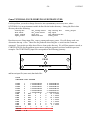
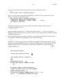
EXODUS II TUTORIAL
1) Change directories into the “tutorial” directory (this location will depend on the course you
are taking and how you installed your software).
2) You will notice a series of files with various extensions. One such file is the in.exoII file.
Issue the following commands:
ncdump in.exoII > dum.txt
more dum.txt
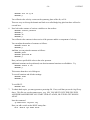
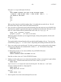
You will notice that this file has a variety of finite element type information, like number of
nodes per element, number of elements, etc.:
-4-
6/12/2015
netcdf in {
dimensions:
len_string = 33 ;
len_line = 81 ;
four = 4 ;
time_step = UNLIMITED ; // (0 currently)
num_dim = 2 ;
num_nodes = 25 ;
num_elem = 4 ;
num_el_blk = 2 ;
num_node_sets = 4 ;
num_side_sets = 5 ;
num_el_in_blk1 = 2 ;
num_nod_per_el1 = 9 ;
num_el_in_blk2 = 2 ;
num_nod_per_el2 = 9 ;
num_nod_ns1 = 5 ;
num_nod_ns2 = 5 ;
num_nod_ns3 = 5 ;
num_nod_ns4 = 5 ;
num_side_ss1 = 2 ;
num_df_ss1 = 6 ;
num_side_ss2 = 2 ;
num_df_ss2 = 6 ;
num_side_ss3 = 4 ;
num_df_ss3 = 12 ;
num_side_ss4 = 2 ;
num_df_ss4 = 6 ;
num_side_ss5 = 2 ;
num_df_ss5 = 6 ;
num_qa_rec = 1 ;
variables:
float time_whole(time_step) ;
long eb_status(num_el_blk) ;
....
This file is clearly a finite element database. You will notice a connectivity array, nodal
coordinates, etc.
3) Next issue the command
ncdump in.gen
You will notice the statement:
ncdump: in.gen: NetCDF: Unknown file format
To summarize this section, these tools are usually needed when a user/developer is trying to understand
in more detail how Goma is interacting and reading/writing these databases, or when a user wants to
extract text-form information from the mesh or data for analysis. In general this is rare.
2. GROPE, ALGEBRA (and FASTQ)
There are many tools in the SEACAS distribution which can be used to generate meshes, manipulate
meshes, and interrogate ExodusII files. Until recently we including SEACAS mesh generator FASTQ
-5-
6/12/2015
in our training, but now it is so obsolete compared to tools like CUBIT that we have relegated that
training module to Appendix A. That said, not everyone has CUBIT, as it is not free, so we felt we
had better keep it. Please consult Appendix A to learn how to use FASTQ/GJOIN/GEN3D. We will
also run FASTQ in other parts of this tutorial, as needed, and even demonstrate a FASTQ translator in
CUBIT.
Some other tools which are worthy of quick mention are:
• GROPE can be used to extract and manipulate EXODUS II files. Often times you want to extract a
value of a variable at a specific location (node) or along a specific side (side set), like pressure
along a permeable substrate, for instance. GROPE can be used to do this. The documentation is
fairly complete and easy to understand.
• ALGEBRA is similar to GROPE but allows you to define other variables based on your current
nodal variable set. For instance, you may want to plot only dimensional quantities, even though
your EXODUS file contains nondimensional ones. In ALGEBRA, you can define dimensional
versions and output a new EXODUS file with those versions to be plotted by BLOT. Again, the
documentation for ALGEBRA is complete and easy to understand
3. CUBIT
CUBIT is a two- and three-dimensional finite element mesh generation toolkit. The CUBIT
Development Team at Sandia National Laboratories has developed and maintains this toolkit for the
most part. But since 2005 or thereabouts CUBIT is being distributed with commercial licenses for a fee.
Toolkit and licensing information for CUBIT can be found at their website: http://cubit.sandia.gov and
also at www.csimsoft.com
The CUBIT Development Team hosts biannual training classes (Introductory and Advanced) so we will
not attempt to duplicate these sessions. Our purpose here is to provide rudimentary skills to carry a user
through the required mesh development stage necessary for Goma training.
CUBIT can be run in three modes - interactive with a graphical user interface (GUI), interactive via
command line, and batch mode. This brief introduction to CUBIT will use the interactive command line
method of data entry/mesh development. We will duplicate mesh development for the simple 2D box
problem.
The primary steps in creating a finite element mesh with CUBIT are geometry creation, interval and
scheme specification, meshing the geometry, assigning boundary flags and exporting the mesh. These
are detailed below. Note the following text format used here: commands entered by the user are in bold
print while responses/echoes from CUBIT are in bold italics print.
1. Geometry Creation:
The topological entities in CUBIT consist of vertices, curves, surfaces, volumes and bodies, each with a
corresponding dimension to it. Each topological entity is bounded by one or more entity of lower
dimension. A body is not required for a complete topological model but is a convenient mechanism for
grouping volumes. Geometries can be created in CUBIT by one of three primary methods: built up from
-6-
6/12/2015
a set of geometry primitives, such as spheres or bricks; defined from the “bottom up” by creating
vertices, then curves, etc.; or finally by importing an ACIS “.sat” file (which forms the solid model
portion of CUBIT).
A simple box is meshed by the following commands using the geometry primitives. As CUBIT is fully
3D by default, a simplistic approach is used to limit graphical displays to two dimensions, i.e., change
the display mode.
graphics mode hiddenline
To create a 1-by-1 box
create brick x 1 y 1
brick body 1 successfully created
Journaled Command: create brick x 1 y 1
This gives us the basic geometry, a set of vertices with connecting line segments defining an enclosed
region. In CUBIT, this entity is a volume. We can check the numbering of the created entities by using
various label options. Look at vertices, curves and volumes, turning off the labeling on the previous
entity before proceeding to the next.
label vertex
label off
label curve
label off
label volume
graphics mode wireframe
The return to “wireframe” mode allows the user to view the volume number placed at the centroid of the
body, a value that cannot be seen when “hiddenline” mode obscures the third dimension.
label off
graphics mode hiddenline
label surface
display
This final display shows the portion of the body we will mesh, i.e., surface 1.
2. Intervals and Scheme:
Element size can be controlled by specifying the mesh density for a particular entity; in this case, we
will use the surface. Meshing scheme is left to default; CUBIT has a set of algorithms that use
topological and geometry data to select the best meshing tool.
surface 1 size .5
Journaled Command: surface 1 size .5
-7-
6/12/2015
3. Meshing:
This is an extremely simplistic mesh so it does not illustrate the capabilities or the options present in
CUBIT. After specifying the parameters and option in step 2, meshing is carried out by specifying a list
of entities to mesh; as above, we use the surface of the volume.
mesh surface 1
Matching intervals successful.
Meshing Surface 1 (Surface 1)
Generated 4 elements for Surface 1 (Surface 1).
Surface 1 (surface 1) meshing completed using scheme: map
Journaled Command: mesh surface 1
The alternate “bottom up” method to reach the same stage can be executed with the following
commands; these are listed only for illustration and comparison (unless you wish to investigate CUBIT
further).
create vertex 0 0
Creation of Vertex 1 (Vertex 1) Successful.
Journaled Command: create vertex 0 0
create vertex 1 0
Creation of Vertex 2 (Vertex 2) Successful.
Journaled Command: create vertex 1 0
create vertex 1 1
Creation of Vertex 3 (Vertex 3) Successful.
Journaled Command: create vertex 1 1
create vertex 0 1
Creation of Vertex 4 (Vertex 4) Successful.
Journaled Command: create vertex 0 1
create curve 1 2
Creation of Curve 1 (Curve 1) Successful.
Journaled Command: create curve 1 2
create curve 2 3
Creation of Curve 2 (Curve 2) Successful.
Journaled Command: create curve 2 3
create curve 3 4
Creation of Curve 3 (Curve 3) Successful.
Journaled Command: create curve 3 4
create curve 4 1
Creation of Curve 4 (Curve 4) Successful.
Journaled Command: create curve 4 1
create surface 1 2 3 4
Creation of Surface 1 (Surface 1) Successful.
This is sheet body 1 (Body 1)
Journaled Command: create surface 1 2 3 4
-8-
6/12/2015
surface 1 size .5
Journaled Command: surface 1 size .5
mesh surface 1
Matching intervals successful.
Meshing Surface 1 (Surface 1)
Generated 4 elements for Surface 1 (Surface 1).
Surface 1 (surface 1) meshing completed using scheme: map
Journaled Command: mesh surface 1
4. Boundary Flags:
Sandia’s EXODUS II format groups mesh information for elements and collections of nodes and
element sides. These collections are termed Element Blocks, Node Sets and Side Sets, respectively.
These are referenced in an analysis code by calling out a designation (i.e., an ID) assigned to these
collections by the mesh generation software.
block 1 surface 1
Assigning Surface 1 to Element Block 1.
Journaled Command: block 1 surface 1
block 1 element type quad4
Journaled Command: block 1 element type quad4
nodeset 1 curve 1
Journaled Command: nodeset 1 curve 1
nodeset 2 curve 2
Journaled Command: nodeset 2 curve 2
nodeset 3 curve 3
Journaled Command: nodeset 3 curve 3
nodeset 4 curve 4
Journaled Command: nodeset 4 curve 4
sideset 1 curve 1
Journaled Command: sideset 1 curve 1
sideset 2 curve 2
Journaled Command: sideset 2 curve 2
sideset 3 curve 3
Journaled Command: sideset 3 curve 3
sideset 4 curve 4
Journaled Command: sideset 4 curve 4
5. Export Mesh:
Setup and creation of the mesh has been completed; all that remains is to save the mesh data into an
appropriately named file. (Note, the filename must be in single quotes.)
export genesis ’box.exoII’ overwrite
File box.exoII will be written with the following version of EXODUS II:
API version:
3.220000
DB version:
2.050000
Preparing genesis mesh data ...done
Preparing genesis side set data . . .1.2.3.4. done
Initializing genesis file...done
Writing coordinates....done
-9-
Writing
Writing
Writing
Writing
Writing
Writing
6/12/2015
element blocks...1...done
nodesets...1.2.3.4...done
sidesets...1.2.3.4...done
global order map...done
global element order map...done
global nodal order map...done
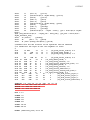
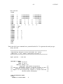
Executive Genesis summary:
number dimensions
= 2
number nodes
= 9
number elements
= 4
number element blocks = 1
number NodeSets
= 4
number SideSets
= 4
Detailed Genesis summary:
-------- Element Block Information ----------Block 1 contains 4 exported 2D element(s) of type QUAD4.
Owned Entities:
______Name______ Type________Id Mesh_Elements
Surface 1 Surface
1
4
-------- NodeSet Information ----------------NodeSet 1: contains 3 nodes.
Owned Entities:
______Name______ Type________Id Mesh_Elements
Curve 1 Curve
1
3
NodeSet 2: contains 3 nodes.
Owned Entities:
______Name______ Type________Id Mesh_Elements
Curve 2 Curve
2
3
NodeSet 3: contains 3 nodes.
Owned Entities:
______Name______ Type________Id Mesh_Elements
Curve 3 Curve
3
3
NodeSet 4: contains 3 nodes.
Owned Entities:
______Name______ Type________Id Mesh_Elements
Curve 4 Curve
4
3
-------- SideSet Information ----------------SideSet 1 contains 2 exported element sides.
Owned Entities:
______Name______ Type________Id Mesh_Elements
Curve 1 Curve
1
2
Sense
All
SideSet 2 contains 2 exported element sides.
Owned Entities:
______Name______ Type________Id Mesh_Elements
Sense
- 10 -
Curve 2
Curve
2
6/12/2015
2
All
SideSet 3 contains 2 exported element sides.
Owned Entities:
______Name______ Type________Id Mesh_Elements
Curve 3 Curve
3
2
Sense
All
SideSet 4 contains 2 exported element sides.
Owned Entities:
______Name______ Type________Id Mesh_Elements
Curve 4 Curve
4
2
Sense
All
Finished writing box.exoII
Removed 0 temporary NodeSets.
Journaled Command: export genesis "box.exoII"
Thus are the basic steps followed for a typical problem. If you want to iterate on the mesh, the current
mesh can be eliminated via
delete mesh
...deleting 4 faces and 16 EdgeUses from database...
...deleting 12 edges from database...
...deleting 9 nodes from database...
Journaled Command: delete mesh
A new mesh density can be selected
surface 1 size .2
or intervals can be specified along particular curves
surface 1 size .2
Journaled Command: surface 1 size .2
curve 1 interval 7
Journaled Command: curve 1 interval 7
curve 2 interval 10
Journaled Command: curve 2 interval 10
curve 2 scheme bias factor 1.2 start vertex 2
Journaled Command: curve 2 scheme bias factor 1.2 start vertex 2
surface 1 scheme pave
Journaled Command: surface 1 scheme pave
mesh surface 1
Matching intervals successful.
Meshing Surface 1 (Surface 1)
Paver grid cell factor changed to 5.2 for surface 1.
..........
Cleaning up paved mesh..
- 11 -
Smoothing
Generated
Surface 1
Journaled
6/12/2015
Surface Mesh...
45 elements for Surface 1 (Surface 1).
(surface 1) meshing completed using scheme: pave
Command: mesh surface 1
Of course CUBIT is a very sophisticated solid-model/meshing package and we highly recommend their
tutorials and their courses, which are very valuable.
4. APREPRO
APREPRO (“A PRE-PROcessor”) is a tool that can be used to parameterize problems in terms of more
familiar quantities. Basically, it is a text processor which allows the user to evaluate expressions and
define variables according to a prescribed syntax. The output is also a text file which has all prescribed
APREPRO syntax removed. Clearly, we can use this tool to generate input files (or “decks”) for CUBIT
and Goma. In this section we will give one brief example of how APREPRO can be used to
parameterize a coating problem in terms of more familiar quantities, but we highly encourage you to
read the manual insert in your documentation and study the tutorial examples below to get a feel for the
extent of its capabilities.
APREPRO TUTORIAL
Suppose we wanted to parameterize a two-layer slide coating flow in terms of quantities like inlet flow
rate (or final film thickness), slide inclination angle, web angle with vertical, coating nip, slide length,
etc. Goma and CUBIT require hard numbers to be input for geometry description (i.e. points and lines)
and velocity boundary conditions. One of APREPRO’s many useful features is that it can be used to
evaluate simple arithmetic expressions and substitute the results where appropriate. The basic syntax is
that any expression in curly braces “{}” is evaluated and the result is substituted upon output. This
example illustrates the concept (please read the APREPRO manual for other more extensive features).
SLIDE COATING DEFINITION FILE (FILE Defs)
$
$
$
$
$
$
$
$
$
$
$
$
$
$
$
$
$
$
$
Thermo-Physical Properties
(all units mks)
viscosity
density
surface tension
gravity
OPERATING CONDITIONS
final thickness layer 1
final thickness layer 2
webspeed
flowrate layer 1
flowrate layer 2
slide angle with horizontal
angle of web and gravity vector
{visc1 = 0.01}
{visc2 = 0.01}
{densi1 = 1.e3}
{densi2 = 1.e3}
{st1
= 0.07}
{st2
= 0.07}
{grav = 9.8}
{finth1
= 45.e-6}
{finth2
= 45.e-6}
{websp = 1.}
{q1
= websp*finth1}
{q2
= websp*finth2}
{alpha = PI/10.}
{beta = 0.}
- 12 -
$
$
$
$
$
$
$
$
$
$
$
$
$
$
$
6/12/2015
CALCULATION OF FILM THICKNESSES
(NB! DENSITIES AND VISC OF BOTH LAYERS ARE THE SAME FOR NOW!)
{cosab = cos(PI/2-alpha+beta)}
{q1a = (q1+q2)/denom}
{thisl1 = (3*q1a)**(1./3.)}
{thisl2 = 0.}
{denom = densi1*grav*abs(cosab)/visc1}
Thin out initial guess a little more
slide film thickness
web film thickness
slide length
web length from top of slide
coating nip (die face and web)
{h1 = thisl1+thisl2}
{h2 = (finth1+finth2)}
{S = 7.0*h1}
{W = 3.0*h1}
{G = 0.4*h1}
$ MESH PARAMETERS
$
${no_elem_along_slide = 17}
${no_elem_along_slide1 = 7}
${no_elem_layer_1 = 3}
${no_elem_layer_2 = 3}
${no_elem_across_film = no_elem_layer_1 + no_elem_layer_2}
${no_elem_across_gap = 5}
${no_elem_along_web = 12}
When this tutorial problem was created, we did not use CUBIT to generate mesh. Instead, we employed
FASTQ, a mesh generation program included in SEACAS distribution. As of this time, we have not
updated the tutorial to use a CUBIT journal file for this slide-coater problem. So the syntax below is
that for FASTQ. However, we can run this file through the CUBIT translator for FASTQ. One could
use these same parameter definitions in a CUBIT journal file, of course.
FASTQ (CUBIT) INPUT FILE (slide.fas)
{include(Defs)}
$$$$This section begins the FASTQ input deck section$$$
Point
1
{x1=G} {y1=-S*sin(alpha)}
Point
2
{x2=G+S*cos(alpha)}
{y2=0}
Point
3
{x3=x2-h1*cos(PI/2-alpha)}
{y3=y2+h1*sin(PI/2-alpha)}
$$NB the factor of 2 here is to make the initial guess better
Point
4
{x4=G} {y4=y1+h1/sin(PI/2-alpha)/2}
Point
5
{x5=h2} {y5=G+y4}
Point
555
{x4+(x4+x5)/3.} {(y4+y5)/2. }
Point
8
{x8=0} {y8=-S*sin(alpha)+G}
Point
6
{x6=h2} {y6=W+y8}
Point
7
{x7=0} {y7=W+y8}
Point
9
{x9=0} {y9=y5}
Point
20
{x20=(x2+x3)/2} {y20=(y2+y3)/2}
Point
21
{x21=x1}
{y21=(y1+y4)/2}
Point
22
{x22=(x8+x4)/2} {y22=(y8+y4)/2}
Point
23
{x23=(x5+x9)/2} {y23=(y5+y9)/2}
Point
24
{x24=(x6+x7)/2} {y24=(y6+y7)/2}
- 13 -
6/12/2015
Point
30
{x30=G+S*cos(alpha)/3} {y30=-S*2*sin(alpha)/3}
Point
32
{x32=G+S*cos(alpha)/3-h1*cos(PI/2-alpha)}
{y32=y30+h1*sin(PI/2-alpha)/2}
Point
31
{x31=(x32+x30)/2}
{y31=(y32+y30)/2}
$ Kramers rule for the solution of two equations and two unknowns
$ is needed for the input of the line segments to salsa.
$
Line
1
STR
2
30
0
{no_elem_along_slide1} 1.
Line
100
STR
30
1
0
{no_elem_along_slide}
0.95
Line
2
STR
2
3
0
{no_elem_across_film}
1.0
Line
3
STR
3
32
0
{no_elem_along_slide1}
1.0
Line
300
STR
32
4
0
{no_elem_along_slide}
0.95
Line
4
CIRC
5
4
555
{2*no_elem_across_gap}
.9
$$Line 4
STR
4
5
0
{no_elem_across_gap}
1.0
Line
5
STR
5
6
0
{no_elem_along_web}
1.2
Line
6
STR
6
7
0
{no_elem_across_film}
1.0
Line
7
STR
7
8
0
{no_elem_along_web+no_elem_across_gap}
1.0
Line
8
STR
8
1
0
{no_elem_across_gap}
1.0
Line
10
STR
4
1
0
{no_elem_across_film}
1.0
Line
11
STR
4
8
0
{no_elem_across_ film}
1.0
Line
12
STR
5
9
0
{no_elem_across_film}
1.0
Line
13
STR
8
9
0
{no_elem_across_gap}
1.0
Line
14
STR
9
7
0
{no_elem_along_web}
1.2
Line
20
STR
20
31
0
{no_elem_along_slide1} 1.0
Line
200
STR
31
21
0
{no_elem_along_slide}
.95
Line
21
STR
21
22
0
{no_elem_across_gap}
1.0
Line
22
STR
22
23
0
{no_elem_across_gap}
1.0
Line
23
STR
23
24
0
{no_elem_along_web}
1.2
Line
30
STR
2
20
0
{no_elem_layer_1}
1.0
Line
31
STR
20
3
0
{no_elem_layer_2}
1.0
Line
32
STR
24
7
0
{no_elem_layer_1}
1.0
Line
33
STR
24
6
0
{no_elem_layer_2}
1.0
Line
34
STR
1
21
0
{no_elem_layer_1}
1.0
Line
35
STR
21
4
0
{no_elem_layer_2}
1.0
Line
36
STR
9
23
0
{no_elem_layer_1}
1.0
Line
37
STR
23
5
0
{no_elem_layer_2}
1.0
Note that the Defs file defines all sorts of well-known quantities, like thermophysical properties and
slide coating geometry. Of course all of this is needed to prescribe the initial geometry that must be
meshed up. So these quantities are then manipulated into film thicknesses, flow rates and
eventually into point and line locations, however this is done in the slide.fas file in which file
Defs is included. Look at each file to get a feel of how the slide.fas depends on Defs. The
geometry description of the FASTQ input file starts below these definitions. In this case, we
include the Defs file in the FASTQ input file. CUBIT, when this fastq input file is read in and
translated automatically runs APREPRO. You can also run APREPRO before being read by
CUBIT (FASTQ). That is, as part of this tutorial, issue the command
aprepro slide.fas dum.fas
- 14 -
6/12/2015
Now look at dum.fas with “more dum.fas” and you’ll see that the point and line commands have
been evaluated and dum.fas is ready to be read into fastq. To automatically send these definition
files “Defs ” and “slide.fast” through this step without execution of APREPRO secperately,
just run CUBIT with an import of slide.fas, which in turn includes the Defs file:
cubit
From the command line window:
CUBIT> import fastq ‘slide.fas’
or you can import the aprepro’d file:
CUBIT. import fastq ‘dum.fas’
That is, CUBIT automatically processes APREPRO syntax. Most of the tools in SEACAS which
take or read in text input files support a “-a” option, which automatically runs the text input file
through APREPRO before reading the file. FASTQ and Goma are two such tools, as is
demonstrated here and below.
5. BLOT - A postprocessor
The BLOT program can be used to visualize an EXODUS II file by displaying the mesh and
vector/contour plots of various quantities. It even allows for time history plots of quantities from
particular points and some simple x-y plots from slices in the domain. It supports several device drivers,
including X-windows (the default and what you will be looking at on your screen) and postscript (for
obtaining hard copies). BLOT is NOT for high-end, high-quality graphics, and some have said that it
will become obsolete by 1995. Well, here we are in 2015 and BLOT is used extensively at Sandia, for
no other reason than it is a quick-and-dirty visualizer that takes no memory, no start-up time and is
expedient.
Basically BLOT is arranged in a multilayered structure, but its accompanying documentation and online
help facility are not as good. At the upper-most level (called BLOT>) the user has several choices,
including log, for saving a journal file, cmdfile , for reading from a previously saved journal file,
detour, a multidimensional vector and contouring package, tplot, for time history plots, and splot ,
for spatial X-Y plots. You will mostly use detour and hence it is the only subpackage covered in this
tutorial. It should be mentioned that BLOT does not take advantage of hardware graphics cards (i.e.,
for 3D rotation and volume rendering). However, it is an extremely fast graphics package that is more
than adequate for all 2D problems and most 3D problems. This tutorial is designed to teach you some of
the basic necessities.
BLOT TUTORIAL
From the same “tutorial” subdirectory do an “ls ” to list the files and choose an “*.exoII ” file to
visualize. Let’s choose the 3ddie.exoII file generated earlier because it is 3D and can be used to
demonstrate how to do rotations.
1.
To start BLOT with this file
- 15 -
6/12/2015
blot 3ddie.exoII
You will note if you forget the exoII file name or just type “blot” you will get a help page advising
you of all of your options.
2.
Anyway, starting up BLOT results in a popped X-window on your screen. Often times it is nice to
re-position that window so you have a clear view of both your command window and the graphics
window. Now with blot you will see the following prompt:
BLOT>
Your options here are several, but the ones we will demonstrate here are log, cmdfile, and detour .
Type “log” to save a journal file of this session.
BLOT>log
We will use this log file to record all of our BLOT commands and re-execute them in this tutorial.
Type “detour ” to enter the contouring and vectoring subroutine:
BLOT>det*our
Note that you need only type “det ”
3.
You have many options here, but the first is to see what variables you have available to you for
plotting. You can do this one of two ways. When you first entered BLOT you noticed just below
the banner page it listed the nodal variables available. Another way is to issue the command:
DETOUR> list names
which results in
Variables Names:
History:
Global:
Nodal:
VX
VZ
PRESSURE
RMY
Element:
VY
P
RMX
RMZ
Notice here we have three nodal velocity components, a nodal pressure, and three more components
of the residuals of the momentum equations.
4.
Once we know what can be plotted lets first look at the mesh. This is default but can be forced at
any time with the “wire” command:
DETOUR> wire
DETOUR>p
These two commands will show you the mesh from a viewing angle parallel with the z-axis.
To rotate the view, use the rotate commands, viz.
DETOUR> rotate x 45
DETOUR> rotate y 45
DETOUR> p
5.
Now let’s look at the velocity vectors. To do this issue the commands:
- 16 -
6/12/2015
DETOUR> vect vx vy vz
DETOUR> p
You will notice the velocity vectors on the symmetry plane of the die, at Z=0.
There are ways to slice up the domain and look at so-called hedge-hog plots but those will not be
covered here.
6.
Now look at the contours of various variables over the surfaces:
DETOUR>
DETOUR>
DETOUR>
DETOUR>
contour pressure
p
vx
p
You will notice the contours in these series of the pressure and the x-component of velocity.
You can adjust the number of contours as follows:
DETOUR> ncntrs 40
DETOUR> p
And then you can paint the contours as follows:
DETOUR> paint
DETOUR> spectrum 40
DETOUR> p
Here you have specified 40 colors to the color spectrum.
Additional rotations can be performed; note that incremental rotations are all additive. Try
DETOUR> rotate x -90
DETOUR> p
This rotates about the x-axis 90 degrees.
To reset all rotations and all other settings:
DETOUR> reset
DETOUR> p
To exit BLOT:
DETOUR> exit
7.
To obtain hard copies, you must generate a postscript file. First, recall that you saved a log file up
above. This file was saved as 3ddie.blot.log. N.B. YOU MUST COPY THIS FILE INTO
ANOTHER NAME BEFORE YOU START UP BLOT AGAIN, OR IT WILL GET BLOWN
AWAY.
Issue the command
cp 3ddie.blot.log blot.log
Here you add a switch on the BLOT startup line:
blot -device cps 3ddie.exoII
- 17 -
6/12/2015
Here we will re-execute all of the BLOT commands by loading the log file:
BLOT> cmdfile blot.log
You will notice that BLOT automatically executes the commands in the log file, which we
encourage you to look at, and exits automatically. List the files in the directory and you will notice
a file called 3ddie.ps. This is the postscript file that can be sent to a printer.
8.
One final trick, and something that can be added to a Frequently Asked Questions (FAQ) list:
To remove all of the border axes, version information and frame of the plot in the postscript file so
that the file might be cleanly imported into a wordprocessing document, can be accomplished in
two ways. The first is to just do a screen capture of the plot while running BLOT in the X-window
default mode. Most Unix systems have this capability, like xwd etc. which can produce a bit map
file that can be cropped or edited. This approach is highly machine dependent. Some word
processing software also supports this utility, like FrameMaker (capture command from the file
utility menu).
Perhaps an easier way is to issue the following commands in DETOUR upon entering:
DETOUR>
DETOUR>
DETOUR>
DETOUR>
legend off
qa off
axis off
outline off
Any plotting performed subsequent to these commands will not have these features. You may want
to leave the legend on and turn the others off.
9.
Seriously, this is the last trick. When visualizing a transient data set, BLOT scales the min and
max for contouring globally. This means if a field is evolving over time, e.g. a temperature is
rising from zero to over 1000 deg. C, then the contours on all time planes are scaled from 0 to 1000.
This means that on early time planes you will not see any variation if that variation is small relative
to the {max T - min T}. To scale each time-plane on its own min and max, simply issue the
following toggle:
DETOUR> cgl
I have no idea what “cgl” stands for.
6. Goma Introduction
This section is intended to give you a brief working introduction to Goma. In most cases, all
information here can be found in the Goma user’s manual and you are encouraged to have a close look
at that and have it on hand as you go through this introductory tutorial. This section is more-or-less a
synopsis of the manual. We will describe here the necessary details of each part of the input and
material files. A separate chapter is devoted to each in the manual, so again this is intended to give you a
quick feel for the input files. Reference to relevant sections of the manual are made in the clips from
computer input files; these references will be seen as section numbers from the Goma manual in an italic
font enclosed in parentheses near the right margin (e.g., (Section 4.1) ).
- 18 -
6/12/2015
The first example on knife coating illustrates the use of APREPRO, multiple material conjugate
problems, and a continuation strategy. The second problem is a substrate-film drying problem. This
problem models a drying film on a flexible substrate which curls as a result of volume shrinkage. We
run this in both a steady state and transient mode to demonstrate many additional features of Goma.
7. Goma TUTORIAL ON KNIFE COATING
In the tutorial directory there is a subdirectory called “knife”. Change directories into knife and view
the files. You will notice files called geometry and knife_input . This first task is to discuss the details
of these files, so you understand what it takes to run this problem. The file geometry actually serves
two purposes: one is to define or parameterize the problem in terms of familiar quantities, like knife
angle, bevel angle, coating speed, etc., and the second is to serve as a CUBIT (FASTQ) input file for the
mesh. Recall from the APREPRO tutorial that you could make this two files: one “definitions” file and
one CUBIT (FASTQ) input file. Using the APREPRO include statement, the definitions file could be
incorporated (by reference) into the CUBIT (FASTQ) input, but in this case we have combined them.
One could certainly convert this FASTQ input file to a CUBIT journal file. That exercise is left to the
reader. The geometry file looks like this:
$Thermo-Physical Properties (all units mks)
$
$ Base viscosity
{visc = 0.01}
$ density
{densi = 1.e3}
$ surface tension
{st
= 0.03}
$ gravity
{grav = 9.8}
$
$
$ GEOMETRY AND OPERATING CONDITIONS (MKS)
$ gap (leading edge to substrate)
{Gap = 0.0005}
$ blade thickness
{d = 0.002}
$ final thickness guess for geometry
{Gap}
$ bevel angle of blade tip
{alpha = PI/3.2} {alpha_new = PI/3.2}
$ angle of blade face with gravity
{beta = PI/10} {beta_new = PI/10}
$ length of outflow plane
{S = 0.015}
$ height of open boundary
{H = 0.006}
$ distance from tip to inflow bndry
{I = 0.005}
$ substrate thickness (for penetration) {h = 0.0004}
$ webspeed
{websp = 0.1}
$
$ MESH PARAMETERS
$
${no_elem_along_outflow = 7}
${no_elem_under_blade = 7}
${no_elem_across_layer = 4}
${no_elem_across_inflow = 9}
${no_elem_across_inflow_back_side = 6}
${no_elem_across_pond = 6}
${no_elem_across_substrate = 3}
${no_elem_along_blade = 5}
Point
10
{x10=-I}
{y10=-h}
- 19 -
6/12/2015
Point
11
{x11=-0}
{y11=-h}
Point
12
{x12=d*cos(PI/2.-alpha-beta)} {y12=-h}
Point
13
{x13=S}
{y13=-h}
Point
20
{x20=-I}
{y20=0}
Point
21
{x21=-0}
{y21=0}
Point
22
{x22=d*cos(PI/2.-alpha-beta)} {y22=0}
Point
23
{x23=S}
{y23=0}
Point
30
{x30=-I}
{y30=Gap}
Point
31
{x31=0}
{y31=Gap}
Point
32
{x32=d*cos(PI/2. - alpha - beta)} {y32 = d*sin(PI/2.-alphabeta)}
$$$$ {x32_new=d*cos(PI/2. - alpha_new - beta_new)} {y32_new = d*sin(PI/2.alpha_new-beta_new)}
Point
33 {x33=S}
{y33=Gap}
Point
40
{x40 = -I}
{y40=H}
Point
41 {x41=-(H-Gap)*tan(beta)} {y41=H}
$ Kramers rule for the solution of two equations and two unknowns
$ is needed for the input of the line segments to salsa.
$
Line
10 STR
10
11
0
{no_elem_across_inflow} 0.8
Line
11
STR
11
12
0
{no_elem_under_blade} 1.
Line
12
STR
12
13
0
{no_elem_along_outflow} 1.2
Line
Line
Line
Line
Line
Line
Line
Line
Line
Line
Line
Line
Line
20
STR
STR
STR
STR
STR
STR
STR
STR
21
22
40
31
32
100
110
120
200
210
220
240
$$REGION
REGION 1
REGION 2
REGION 3
4
1
1
1
STR
21
22
40
31
32
10
20
41
STR
STR
STR
STR
20
22
23
41
32
33
20
40
31
31
32
33
23
21
0
0
0
0
0
0
0
0
2 -100 -10 -11 -12 -240
-20 -200 -120 -40 -110
-200 -21 -210 -31
-210 -22 -220 -32
BODY 1 2 3
SCHEME
SCHEME
SCHEME
SCHEME
1
2
3
4
21
22
23
13
0
{no_elem_across_inflow} 0.8
{no_elem_under_blade} 1.
{no_elem_along_outflow} 1.2
{no_elem_across_inflow_back_side} 1.0
{no_elem_under_blade} 1.
{no_elem_along_outflow} 1.2
{no_elem_across_substrate} 1.
{no_elem_across_inflow_back_side} 1.
{no_elem_along_blade} 0.8
0
{no_elem_across_layer} 1.
0
{no_elem_across_layer} 1
0
{no_elem_across_layer} 1
0
{no_elem_across_substrate} 1
X
M
M
M
POINBC 100 32
POINBC 200 33
NODEBC {substrate_ns=2} 20 21 22
-22 -21 -20
- 20 -
NODEBC
NODEBC
NODEBC
NODEBC
NODEBC
{inflow_back_ns=3} 110
{inflow_top_ns=4} 40
{blade_face_ns=5} 120
{blade_tip_ns=6} 31
{outflow_plane_ns=8} 220
ELEMBC
ELEMBC
ELEMBC
ELEMBC
ELEMBC
ELEMBC
ELEMBC
{substrate_ss=2} 20 21 22
{inflow_back_ss=3} 110
{inflow_top_ss=4} 40
{blade_face_ss=5} 120
{blade_tip_ss=6} 31
{free_surface_ss=7} 32
{outflow_plane_ss=8} 220
6/12/2015
EXIT
Notice how the points and the lines are expressed in terms of the defined parameters like blade
thickness, gap, bevel angle, etc. Also notice that we have defined names for each ELEMBC, or side set,
and each NODEBC, or node set. That is, after this file is processed with APREPRO those names are
just converted into numbers, but including this file in the Goma input file allows us to refer to the side
set and node set numbers by name.
1.
Let us go ahead and process this file into a mesh. To do this, we need to read it into FASTQ, but not
before we process it through APREPRO, viz.
cubit
CUBIT>
CUBIT>
CUBIT>
CUBIT>
CUBIT>
import fastq ‘geometry’
mesh surface all
block 1 surface all
block 1 element type QUAD9
export genesis ‘knife.exoII’ overwrite
(one could do the same with fastq, following the instructions in APPENDIX
A):
fastq -a geometry
ENTER OPTION: m,ni,op,p,g,p
ENTER MESH GRAPHICS OPTION: ,w
GENESIS DATABASE OUTPUT FILE NAME: knife.gen
ENTER MESH OPTION: exit
(Note here that we turned on the nine-node quad option with ni, and the optimize option with op.
These options are toggle switches, and can be put into the FASTQ input file as a NINE and a RENUM
card, respectively. Make sure you have generated a nine-node quad mesh, i.e, make sure FASTQ
tells you this:
- 21 -
6/12/2015
**************************************************
**
MESH PROCESSING COMPLETED
**
**
THREE NODE BARS OUTPUT
**
**
NINE NODE QUADS OUTPUT
**
**
WITH NODE AND ELEMENT NUMBERING OPTIMIZED **
**
LARGEST NODE DIFFERENCE PER ELEMENT:
52 **
** NODES: 427; ELEMENTS:
92; MATERIALS:
1 **
**************************************************
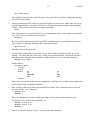
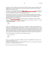
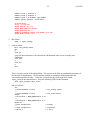
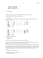
In CUBIT (FASTQ), have a look at the geometry by executing it. Notice that we have a knife, a
pond upstream of the knife, and a well-defined substrate. As it turns out, the substrate is Region 4,
and we currently have that region commented-out in the file (see the first double underlined region
card above). That is, we are not going to solve any equations in the substrate. As an extension to
this exercise, though we will grid up the substrate and allow it to deform for now. The annotated
initial meshed geometry is show below.
Knife
Upstream
pond
Substrate
2.
Now we will dissect the Goma input file to make sure we are defining correctly the problem to be
solved. In the tutorial/knife subdirectory, you will notice the file knife_input . Either “more”
or “vi” this file and examine it.
The first section looks like this
{include(geometry)}
-----------------------------------------------------------FEM File Specifications
(Section 4.1)
-----------------------------------------------------------FEM file
= knife.exoII
Output EXODUS II file
= out.exoII
GUESS file
= contin.dat
SOLN file
= soln.dat
Write intermediate results
= no
-----------------------------------------------------------General Specifications
-----------------------------------------------------------Number of processors
= 1
(Section 4.2)
Output Level
= 0
Debug
= 0
Initial Guess
= zero
- 22 -
6/12/2015
Notice that the “geometry” file discussed above is included here, so that several important
parameters regarding geometry and properties can be calculated. The highlights of this section of
the Goma input deck are that we are taking the mesh from the file knife.exoII , writing the results
to out.exoII, and using a zero initial guess. The next two sections are as follows:
-----------------------------------------------------------Time Integration Specifications
(Section 4.3)
-----------------------------------------------------------Time integration
= steady
-----------------------------------------------------------Solver Specifications
(Section 4.7)
-----------------------------------------------------------Solution Algorithm
= umf
Number of Newton Iterations
= 10
Newton correction factor
= 1
Normalized Residual Tolerance
= 1.0e-13
------------------------------------------------------------
Since we have chosen “steady ” for time integration, The “Time Integration Specification ”
section is completely specified. For transient simulation, we need to specify more entries such as
time integration scheme, initial time step, final time, etc. The solution algorithm for the matrix
system that results from the Newton iteration scheme is “umf” which comes from direct solver
UMFPACK. Other options for direct solvers are “lu”, and “amesos”. Amesos is an interface Goma
used to access parallel direct solvers such as SuperLU and MUMPS. See Goma’s user manual for
more details. Iterative solvers are available as well; however, their use for viscous free surface
flows requires pressure stabilization options beyond the scope of this discussion. The
preconditioner cards, polynomial cards, size of Krylov subspace and Orthogonalization cards and
Linear solve iteration cards are all ignored with the “umf ” option. The “Number of Newton
Iterations ” card sets the maximum number of nonlinear iterations. The Newton correction
factor card sets the relaxation factor for each Newton iteration. Conveniently, these can be
overridden from the Goma execute command line, as described in the manual and demonstrated
below. This is handy when making several continuation steps to get within the radius of
convergence.
The next relevant section is the all-important boundary condition section:
-----------------------------------------------------------Boundary Condition Specifications
-----------------------------------------------------------------------------------------------------------------------Related SS bc’s on position
------------------------------------------------------------$ SET c’s to zero for 2D problem
$
{c1=0} {c2=0} {c3=0} {c4=0} {c5=0} {c6=0} {c7=0} {c8=0}
$
$ Calculate coefficients for general equation a*x + b*y +c*z +d = 0
$
$
{a2=(y20-y23)/(x23-x20)}
$
{d2=(-y23-a2*x23)}
- 23 -
6/12/2015
$
{b2=1}
$
$ NB: this is a vertical line
$
{b3=(x20-x40)/(y40-y20)}
$
{d3=-x40-b3*y40}
$
{a3=1}
$ NB: this could be a vertical line
$
{b5=(x41-x31)/(y31-y41)}
$
{d5=-x31-b5*y31}
$
{a5=1}
$
$
{a6=(y31-y32_new)/(x32_new-x31)}
$
{d6=(-y32_new-a6*x32_new)}
$
{b6=1}
Number of BC
BC
BC
BC
BC
BC
BC
=
=
=
=
=
=
BC
BC
= U NS 2 {websp}
= V NS 2 0.
BC
= V NS 3 0.
BC
= V NS 4 0.
PLANE
PLANE
PLANE
PLANE
PLANE
PLANE
SS
SS
SS
SS
SS
SS
2
3
4
5
6
8
= -1
{a2} {b2} {c2}
{a3} {b3} {c3}
0. 1. 0. -{H}
{a5} {b5} {c5}
{a6} {b6} {c6}
1. 0. 0. {-S}
{d2}
{d3}
{d5}
{d6}
BC
BC
= U NS 5 0.
= V NS 5 0.
BC
BC
= U NS 6 0.
= V NS 6 0.
BC
$$BC
$$BC
$$BC
= VELO_NORMAL SS 7 0.
= KINEMATIC SS 7 0.
= CAPILLARY SS 7 1. 0. 0. 0.
= CAP_ENDFORCE NS 200 1. 0. 0. 1.0
$BC
BC
= V NS 8 0.
= VELO_TANGENT SS 8
0
0. 0. 0.
BC = DX NS 100 {x32_new - x32} 1.0
BC = DY NS 100 {y32_new - y32} 1.0
END OF BC
Here we will discuss the double-underlined cards in this section, as they are the most important.
• The first set of cards is used to compute the slopes and intercepts of the straight lines used to define
- 24 -
6/12/2015
the geometry. These coefficients are needed on the PLANE geometric boundary conditions below.
Notice how these coefficients depend on the geometrical point locations that were defined with
APREPRO in the geometry file.
• The next line with a double underline is the Number of BC
= -1 card. Here you
can either specify the number of boundary condition cards to be read, or just specify -1, in which
case it will read all BC cards between it and the END OF BC card.
• The first set of BCs pertains to the geometry. The PLANE boundary conditions specify that the
mesh along that plane must remain on the plane, but may slide frictionlessly along it. Note that the
coefficients depend on the original geometry, but that the geometry may be changed without
regenerating the mesh, as shown below.
• Note that the BC = U NS 2 {websp} card specifies that the x-component of velocity along the
substrate is set at the web speed, defined in the geometry file. This substrate is node set 2. To verify
quickly that this is node set 2, run BLOT as follows:
blot knife.exoII
det
nset 2
p
• The next set of highlighted cards contains the VELO_NORMAL condition and the KINEMATIC
condition. The first step of obtaining a solution here is to do so on a fixed grid. In this case we need
to comment out the KINEMATIC card (note that we use $$ in the first two columns, but you can do
whatever you want), and solve the equations with the VELO_NORMAL boundary condition. The
VELO_NORMAL condition specifies that no penetration is allowed across that side set (in this case
side set 7) but in the absence of any other conditions allows the fluid to slip freely along the side
set. Run BLOT again to verify that this is the downstream meniscus:
blot knife.exoII
det
sset 7
p
• Below we will change out the VELO_NORMAL condition for the KINEMATIC condition when
we allow the surface to go free.
• Finally the CAPILLARY card and the CAP_ENDFORCE card are used to apply surface tension to
the surface. We will demonstrate these below.
•
The next relevant section is that of the Problem Description:
- 25 -
6/12/2015
###########
---Problem Description
---
(Section 4.12)
Number of Materials = 1
MAT = coating_liq
1
Coordinate System = CARTESIAN
Mesh Motion = ARBITRARY
Number of bulk species = 0
Number of EQ
EQ = mesh1
EQ = mesh2
EQ = momentum1
EQ = momentum2
EQ = continuity
Q1
Q1
Q2
Q2
P1
D1
D2
U1
U2
P
= 5
Q1
Q1
Q2
Q2
P1
0.
0.
0.
0.
1.
div
ms
0.
0.
1.
1.
0.
0.
1.
1.
1.
1.
1.
1.
adv
bnd
dif
0.
0.
0. 0.
0. 0.
0.
src porous
Notice here that the material file from which Goma will seek the material properties is called
coating_liq.mat . Also notice that the block number is 1, and this number corresponds to the
material number input on the region card in FASTQ. By the way, you should have a look at this
material file to see how the properties are input. Also notice that this is a CARTESIAN simulation
with ARBITRARY mesh motion. Rather than go into details here, please refer to the manual for the
purpose of these cards. What is important to point out here, however, is the number of equations
and materials. In this simulation, we have one material (coating_liq.mat ) in which we will solve
5 differential equations. The two mesh equations (mesh1 and mesh2 ) are needed to move the mesh
as a pseudo-solid. Notice that we chose Q1 for the interpolation and the Galerkin weighting
function, which means that we use one-order lower basis functions for the mapping, while
maintaining a biquadratic element for the velocities, i.e., Q2. The names of the variables U1, U2,
D1, D2, and P are not arbitrary, so please adhere to what the manual allows for now.
Finally, the floating point constants on the equation specification lines are term multipliers, which
are mainly used for research purposes. These multipliers are typically set to zero or one, depending
on whether you want the term on or off. Each column of multipliers refers to a particular term, as
indicated by the “div ms adv bnd... ” comment line. Actually, if any physical property multiplies
a term, like density on a convective term, the multiplier also multiplies the same term. i.e., it is not
recommended to use these terms to input physical properties, although one could.
The remainder of the Goma input deck specifies output for the resulting EXODUS II file,
out.exoII in this case, including specific user-selected auxiliary fields that will be computed. You
can read about these cards in the manual.
3.
Now it is time to run this knife coating problem. First we will get a solution on a fixed grid. For this
we will leave the knife_input file as is and execute:
Goma -a -i knife_input
- 26 -
6/12/2015
Note that we use the -a switch to head knife_input and coating_liq.mat through APREPRO
before Goma. After several screens worth of informational junk which we will eventually put into a
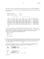
file, you will see:
Number of unknowns
= 1374
Number of matrix nonzeroes
= 70646
R e s i d u a l
ToD
-------17:13:35
17:14:05
17:14:14
17:14:23
17:14:32
17:14:40
itn
--[0]
[1]
[2]
[3]
[4]
[5]
L_oo
------2.2e-04
1.6e-04
3.6e-05
6.7e-07
2.1e-10
1.5e-17
L_1
------7.6e-03
5.8e-03
1.3e-03
1.9e-05
5.5e-09
5.3e-16
C o r r e c t i o n
L_2
------7.8e-04
5.4e-04
1.4e-04
2.2e-06
6.4e-10
5.2e-17
L_oo
------2.5e+01
2.0e+00
6.3e-02
1.3e-03
6.8e-07
3.5e-14
L_1
------9.2e+02
7.2e+01
2.9e+00
7.1e-02
4.0e-05
2.2e-12
L_2
lis asm/slv (sec)
------- --- --------------1.2e+02 1 2.2e-01/5.0e-02
7.7e+00 1 1.8e-01/4.0e-02
2.8e-01 1 1.8e-01/3.0e-02
7.1e-03 1 1.9e-01/3.0e-02
4.1e-06 1 1.9e-01/3.0e-02
2.1e-13 1 1.9e-01/3.0e-02
-done
Note the strong convergence in all norms, both the Residual norms (the first 3 columns) and the
Newton update norms (columns 4 through 6). The numbers under the asm/slv (sec) column are the
cpu time it takes to assemble the residual equations and solve the resulting matrix system,
respectively. You should look at this result quickly with:
blot out.exoII
det
vect vx vy
p
cont stream
p
4.
The next step is to do a little zeroth order continuation to release the meniscus and get a free surface
flow. Notice that the continuation file in the knife_input deck is soln.dat. To read it in, copy
soln.dat into contin.dat and edit the input file Initial Guess card to reflect “read ”, i.e.,
Initial Guess
= read
We also need to release the free surface. To do this comment out the VELO_NORMAL card and
uncomment the KINEMATIC card in the knife_input file, i.e., change this
BC
$$BC
$$BC
= VELO_NORMAL SS 7 0.
= KINEMATIC SS 7 0.
= CAP_ENDFORCE NS 200
1. 0. 0. {st}
to
$$BC
BC
BC
= VELO_NORMAL SS 7 0.
= KINEMATIC SS 7 0.
= CAP_ENDFORCE NS 200 1. 0. 0. {st}
Save the file.
- 27 -
6/12/2015
Now, before we continue, it is important to understand that this is a moving mesh problem and
often times with Newton’s method we need to take a few “relaxed” steps to get to a solution. Of
course you usually guess wrong on the first try on how relaxed to make the steps and how many
relaxed steps to take, but we know this works:
Goma -a -i knife_input -r 0.1 -n 7
,
followed by five steps of -r 0.8 Newton iteration (notice the use of the -n option to override the
specification of the Max. Number of Newton Iterations in the input deck):
cp soln.dat contin.dat
Goma -a -i knife_input -r 0.8 -n 5
,
followed by a few steps of full Newton:
cp soln.dat contin.dat
Goma -a -i knife_input
Now look at the results and you will see that the surface has “sagged” and you now have a
development zone.
blot out.exoII
det
cont stream
p
5.
Now we will alter the geometry a bit, without regenerating the original mesh. First, change the
bevel angle of the blade in the geometry file:
Change
$ bevel angle of blade tip
{alpha = PI/3.2} {alpha_new = PI/3.2}
$ bevel angle of blade tip
{alpha = PI/3.2} {alpha_new = PI/4.2}
to
Let us first try a full Newton step:
cp soln.dat contin.dat
Goma -a -i knife_input
Notice again the strong convergence. Have a look at the results again with BLOT and notice that
the bevel face is much steeper.
- 28 -
6/12/2015
Goma TUTORIAL ON FILM DRYING-SUBSTRATE CURL
For this problem you need to change directories into $(TUTORIAL)/tutorial/curl , where
$(TUTORIAL) is an environment variable defined for the header directory. Listing (ls) files in that
directory shows the following:
coating.mat
film.exoII
input_steady
input_trans
out_steady.exoII
out_trans.exoII
soln.dat
substrate.mat
tmp.coating.mat
tmp.input
tmp.substrate.mat
trans_error
trans_ou tput
Here there are two Goma input files: input_steady and input_trans. We will discuss each case.
Also notice the tmp.* files. These files are produced when using the -a switch on the Goma run
command. You can always delete these files to clean up the directory. We will first generate a mesh, or
CUBIT/FASTQ file for the problem (film.exoII ) using the approach you have learned in previous
examples. The CUBIT/FASTQ input file corresponds to the following geometry:
4
FILM
4
1
5
2
1
SUBSTRATE
5
6
and has an input file (film.fas) that looks like:
TITLE
SUBSTRATE CURL PROBLEM
POINT
POINT
POINT
POINT
POINT
POINT
LINE
LINE
LINE
LINE
LINE
LINE
LINE
REGION
REGION
SCHEME
3
3
1
2
3
4
5
6
1
2
3
4
5
6
7
1
2
0 M
0.0000000E+00
1.0000000E+01
1.0000000E+01
0.0000000E+00
0.0000000E+00
1.0000000E+01
STR
1
2
STR
2
3
STR
3
4
STR
4
1
STR
1
5
STR
5
6
STR
6
2
1
-1
-2
2
-6
-7
0.0000000E+00
0.0000000E+00
1.0000000E+00
1.0000000E+00
-5.0000000E-01
-5.0000000E-01
0
10 0.7000
0
8 1.0000
0
10 1.4200
0
8 1.0000
0
2 1.0000
0
10 0.7000
0
2 1.0000
-3
-4
-1
-5
7
2
6
- 29 -
BODY
POINBC
POINBC
POINBC
POINBC
POINBC
POINBC
NODEBC
NODEBC
NODEBC
NODEBC
NODEBC
NODEBC
NODEBC
ELEMBC
ELEMBC
ELEMBC
ELEMBC
ELEMBC
ELEMBC
ELEMBC
RENUM
NINE
EXIT
1
100
200
300
400
500
600
1
2
3
4
5
6
7
1
2
3
4
5
6
7
6/12/2015
2
1
2
3
4
6
5
1
2
3
4
7
6
5
1
2
3
4
7
6
5
Notice there are two regions and two materials (see REGION cards) and the stretching coefficients that are
used to draw the mesh to the outer edge of the film. The problem here is to clamp the inner edge of the
coating and substrate (left side), dry the film, and follow the overall stress development and
deformation. We will run this problem in two modes. First is the steady state mode. The input deck
for this mode is the file input_steady . Let’s discuss some of the critical parts of that input file. In the
first two sections, two cards are noteworthy:
FEM File Specifications
--FEM file
= film.exoII
Output EXODUS II file
= out_steady.exoII
GUESS file
= contin.dat
SOLN file
= soln.dat
Write intermediate results
= no
--General Specifications
--Number of processors
= 1
Output Level
= 0
Debug
= 0
Initial Guess
= zero
#Initial Guess
= read_exoII
#Initial Guess
= read
Initialize = MASS_FRACTION 0 0.25
(Section 4.1)
(Section 4.2)
- 30 -
6/12/2015
The input finite element database file (film.exoII) is defined on the FEM File card and the initial
mass fraction of component 0 is set to 0.25 with the Initialize card. The next relevant section of
input is boundary condition specification. (Since the problem is being run in the steady state mode
with the umf solver, all other sections are like those in the previous case study. The boundary
conditions look like:
---Boundary Condition Specifications
---Number of BC
=
BC = PLANE SS 4 1.00 0.0 0. 0.0
BC = DX NS 100 0.0
BC = DY NS 100 0.0
BC = PLANE SS 7 1.00 0.0 0. 0.0
BC =
YFLUX
SS
3
0
BC =
YFLUX
SS
2
0
#########
END OF BC
#########
(Section 4.10)
-1
5.
5.
0.25
0.25
Note here that we are pinning node set (i.e. NS) 100 with the DX and DY conditions. This is point 1
in the geometry file and is identified in film.fas as the first POINBC card. You can confirm this
by looking at film.exoII with BLOT and turning on display of nset 100. Also, we are
constraining side sets 4 and 7 (SS 4 and 7; see file film.fas) to stay on the x=0 plane with the
PLANE boundary condition; this is the “clamped” end. Finally, we are specifying a lumped
parameter mass-transfer model along the surface of the film so that the mass flux of Species 0
follows a 5.0*(Concn - 0.25) specification at the surface.
The next section, or problem description section, contains several instructive features:
- 31 -
6/12/2015
---Problem Description
----
(Section 4.12)
Number of Materials = 2
MAT =
coating
1
Coordinate System = CARTESIAN
Element Mapping
= isoparametric
Mesh Motion = LAGRANGIAN
Number of bulk species = 1
Number of EQ = 4
EQ = mesh1
EQ = mesh2
EQ = continuity
EQ = species_bulk
MAT =
substrate
Q2
Q2
P1
Q2
D1 Q2
D2 Q2
P P1
Y Q2
1.
1.
div
0.
0.
0.
0.
0.
0.
1.
1.
1.
ms
1.
adv
1.
bnd
0.
dif
0.
0.
0.
0.
ms
adv
0.
0.
1.
src porous
2
Coordinate System = CARTESIAN
Element Mapping
= isoparametric
Mesh Motion = LAGRANGIAN
Number of bulk species = 0
Number of EQ
= 3
EQ = mesh1
EQ = mesh2
EQ = continuity
Q2 D1 Q2
Q2 D2 Q2
P1 P P1
1.
div
0.
0.
bnd
1.
1.
dif
0.
0.
1.
src porous
You’ll notice that the evolution equations for the coating do not include solution of the momentum
equations for the fluid. This is a solid film/coating which can support a shear stress. There are two
materials, each with a different problem description - a truly conjugate problem. Note that Species
0 is confined to the film only and even though we might have more than one species, we use only
one species_bulk equation. The material files will single out properties of individual species, as
discussed below. The continuity equation contains a source term; this is included in the
formulation to account for the volume shrinkage effect produced by mass loss and to properly
account for the pressure. The mesh motion type is Lagrangian, meaning the mesh moves with the
materials. When the mesh motion is Lagrangian, it will deform according to the prescribed loads
and according to the prescribed constitutive equation in the material file.
There are two materials, and so there MUST be two material files: substrate.mat and
coating.mat . Let us examine each one (use more coating.mat and more substrate.mat ).
First, in coating.mat, you will notice the solid constitutive equation and the properties:
- 32 -
6/12/2015
---Mechanical Properties and Constitutive Equations
Solid Constitutive Equation
= INCOMP_PSTRAIN
#Solid Constitutive Equation
= HOOKEAN_PSTRAIN
Convective Lagrangian Velocity = NONE
Lame MU
= CONSTANT
1.
Lame LAMBDA
= CONSTANT
0.
Stress Free Solvent Vol Frac
= CONSTANT
0.5
(Section 5.2)
The constitutive equation is INCOMP_PSTRAIN , i.e., incompressible plane strain. The fact that it is
incompressible necessitates the solution of the continuity equation and the pressure unknowns. The
Lame MU and Lame LAMDA coefficients are actually Poisson’s ratio and the bulk modulus when
using nonlinear constitutive equations. You’ll notice the shear modulus is zero because the
constitutive equation is incompressible. Lame MU then becomes Young’s modulus.
Finally, the stress-free solvent volume fraction is set to 0.5; this is simply the solvent volume
fraction at which the film is stress free.
The only other significant input in the coating.mat file to discuss is that which specifies the
species diffusivity:
---Species Properties
Diffusion Constitutive Equation
Diffusivity
Latent Heat Vaporization
Latent Heat Fusion
Vapor Pressure
Species Volume Expansion
Reference Concentration
(Section 5.6)
=
=
=
=
=
=
=
FICKIAN
CONSTANT
CONSTANT
CONSTANT
CONSTANT
CONSTANT
CONSTANT
0
0
0
0
0
0
1.
0.
0.
0.
1.
0.
Note that the species number is 0 and the value is 1. If you had more than one species, you would
repeat this group of cards.
In the substrate.mat file, you will notice that the same constitutive equations are employed and
that the substrate is treated as incompressible but with a much higher modulus:
Solid Constitutive Equation
Convective Lagrangian Velocity
Lame MU
Lame LAMBDA
Stress Free Solvent Vol Frac
=
=
=
=
=
INCOMP_PSTRAIN
NONE
CONSTANT
100.
CONSTANT
0.
CONSTANT
0.
Now let us run the steady and transient problems as identified in the 5 steps below:
1.
First generate the mesh:
CUBIT> import fastq ‘film.fas’
CUBIT> mesh surface all
- 33 -
CUBIT>
CUBIT>
CUBIT>
CUBIT>
6/12/2015
block 1 surface 1
block 2 surface 2
block 1 2 element type QUAD9
export genesis ‘film.exoII’
OR WITH FASTQ:
fastq -a film.fas
ENTER OPTION: m,p,g,p
ENTER MESH GRAPICS OPTION: ,
ENTER MESH OPTION: w
GENESIS DATABASE OUTPUT FILE NAME: film.gen
ENTER MESH OPTION: exit
2.
Run Goma:
Goma -i input_steady
3.
Look at results:
blot out_steady.exoII
det
p
cont y0
(you will notice that there is no variation in concentration since we are at steady state
conditions)
cont e22
p
cont t11
p
exit
This is a steady version of the curl problem. The stresses in the film are sustained by resistance of
the substrate to deformation. We can run this problem in a transient fashion and watch the
concentration profiles develop. To do this, you must use the Goma input deck called
input_trans in the same directory. Issue the following UNIX diff command:
diff input_steady input_trans
and you will see
5c5
< Output EXODUS II file
= out_steady.exoII
--> Output EXODUS II file
= out_trans.exoII
18c18
< Initialize = MASS_FRACTION 0 0.25
--> Initialize = MASS_FRACTION 0 0.5
22c22,30
< Time integration
= steady
--> Time integration
= transient
> delta_t
= 1.0e-3
- 34 -
> Maximum number of time steps
> Maximum time
> Minimum time step
> Time step parameter
> Time step error
> Printing Frequency
44,45c52,53
< BC =
YFLUX
SS
3
< BC =
YFLUX
SS
2
--> BC =
YFLUX
SS
3
> BC =
YFLUX
SS
2
=
=
=
=
=
=
6/12/2015
100
10.0e+0
1.0000e-9
0.0
0.002 1 1
1
0
0
5.
5.
0.25
0.25
0
0
5.
5.
0.
0.
1
1
1
1
The differences are clear. We are specifying a higher stress-free solvent volume fraction
(MASS_FRACTION ) and a lower “sink” concentration on the mass transfer coefficient (YFLUX). Also
notice that the Time Integration card was switched to transient and we then supply all the
relevant time integration information. You should consult your manual for the purpose of each
card.
4.
To run the transient version:
Goma -i input_trans
You will notice standard output (to your screen) which looks like:
Number of unknowns
= 1539
Number of matrix nonzeroes
= 81641
Setting MASS_FRACTION number 0 (variable [4]) to 0.5
=> Try for soln at t=0.001 with dt=0.001 [0 for 0] (BE)
N e w t o n
C o n v e r g e n c e
ToD
itn
L_oo
L_1
L_2
-------- --- ------- ------- ------16:32:56 [0] 2.1e-02 9.1e-01 1.1e-01
16:32:58 [1] 2.0e-03 4.2e-02 5.2e-03
16:32:59 [2] 5.9e-04 6.3e-03 1.1e-03
16:32:59 [3] 3.6e-05 2.0e-04 6.0e-05
16:32:59 [4] 1.8e-07 7.0e-07 2.6e-07
16:33:00 [5] 4.3e-12 1.8e-11 6.0e-12
16:33:00 [6] 4.0e-16 1.2e-14 1.0e-15
scaled solution norms
1.013227e+00
- I m p l i c i t
T i m e
L_oo
L_1
L_2
lis
------- ------- ------- --1.0e+00 8.5e+01 8.9e+00 1
2.3e-01 1.8e+01 8.1e-01 1
2.3e-02 5.6e-01 4.1e-02 1
1.5e-03 2.4e-02 2.1e-03 1
1.2e-05 3.8e-05 1.4e-05 1
2.6e-10 8.3e-10 3.4e-10 1
3.4e-14 1.0e-12 1.1e-13 1
1.777290e-01 3.300731e-01
S t e p
asm/slv (sec)
--------------2.4e-01/1.6e+00
2.1e-01/3.4e-01
2.2e-01/2.0e-01
2.1e-01/1.9e-01
2.2e-01/1.9e-01
2.2e-01/1.9e-01
2.1e-01/2.0e-01
CONSTANT DELTA_T
[1.1e-02, 4.1e-03, 1.3e-01]
Predictor-corrector norm: [ 1 d ,
1 y ,
1 P ]
=> Try for soln at t=0.002 with dt=0.001 [1 for 1] (BE)
N e w t o n
C o n v e r g e n c e
- I m p l i c i t
T i m e
S t e p
ToD
itn
L_oo
L_1
L_2
L_oo
L_1
L_2
lis asm/slv (sec)
-------- --- ------- ------- ------- ------- ------- ------- --- --------------16:33:01 [0] 1.3e-02 7.1e-01 7.4e-02 1.0e+00 8.1e+01 8.9e+00 1 2.1e-01/1.9e-01
- 35 -
16:33:01 [1] 2.0e-04 5.4e-03 6.7e-04
16:33:02 [2] 1.8e-06 2.9e-05 3.6e-06
16:33:02 [3] 4.0e-10 2.0e-09 5.7e-10
16:33:02 [4] 3.5e-16 1.3e-14 9.5e-16
scaled solution norms
1.026663e+00
6/12/2015
9.8e-03 3.3e+00 1.5e-01 1
7.6e-05 1.3e-02 5.5e-04 1
1.9e-08 4.5e-06 2.1e-07 1
5.9e-14 1.8e-12 1.4e-13 1
1.858727e-01 3.301558e-01
2.1e-01/1.9e-01
2.1e-01/2.0e-01
2.1e-01/2.0e-01
2.1e-01/2.0e-01
CONSTANT DELTA_T
[2.2e-03, 2.4e-03, 1.3e-01]
Predictor-corrector norm: [ 1 d ,
1 y ,
1 P ]
=> Try for soln at t=0.003 with dt=0.001 [2 for 2] (BE)
N e w t o n
C o n v e r g e n c e
ToD
itn
L_oo
L_1
L_2
-------- --- ------- ------- ------16:33:03 [0] 1.8e-03 9.0e-02 1.0e-02
16:33:03 [1] 1.8e-05 3.8e-04 4.0e-05
16:33:04 [2] 4.1e-09 1.4e-08 4.8e-09
16:33:04 [3] 5.2e-16 1.5e-14 1.2e-15
scaled solution norms
1.039568e+00
- I m p l i c i t
T i m e
L_oo
L_1
L_2
lis
------- ------- ------- --1.3e-02 1.4e+00 6.5e-02 1
1.9e-04 1.4e-02 6.1e-04 1
4.0e-08 4.8e-07 4.6e-08 1
5.8e-14 1.4e-12 1.8e-13 1
1.934510e-01 3.310054e-01
S t e p
asm/slv (sec)
--------------2.1e-01/2.0e-01
2.1e-01/2.0e-01
2.1e-01/2.0e-01
2.1e-01/2.0e-01
The time step starts as 1.e-3 but adjusts (grows or is reduced) according to the error measure
defined by the Time Step Error card. When you look at the results with blot, which are in file
out_trans.exoII , notice that contouring the concentration (Y0) shows the development of
concentration boundary layers, as expected. Also notice that all of the time planes are output into
the EXODUS II file. You can control this with the printing frequency card.
There is much more to glean from all exercises in this tutorial and this document will be continually
updated (see version number on Subject line). This serves as an introduction to Goma and its
associated pre- and post-processors. Questions may be addressed to Randy at [email protected].
APPENDIX: FASTQ, GJOIN, GEN3D
This section introduces and provides a tutorial on mesh generation with FASTQ, GEN3D and GJOIN,
and subsequent database manipulation/interrogation with GROPE and ALGEBRA. You can read about
each of these tools in your SEACAS documentation, as a Sandia Technical Report for each is contained
in that set.
FASTQ is a straight forward two-dimensional mesh generator. It has the ability to produce meshes on
arbitrary shaped domains with both mapped and paved meshes. FASTQ is needed to generate the input
mesh file (an EXODUS II file) for Goma. The tutorial below will instruct you how to do this. As a
take-home assignment here, locate the FASTQ FLOWCHART figure on page 21 of the FASTQ user’s
manual illustrating the layered command structure. Make a photocopy of that page and paste it on your
wall next to your computer. This page is easily the most valuable reference in the manual. NOTE:
Since about 2002 FASTQ is rarely used as a mesh generator as several mainstream geometry-CAD
based mesh generators like PATRANTM, Solid WorksTM, and Sandia’s product and now commercially
avaialble CUBIT. Nonetheless, it is useful to be aware of FASTQ’s capabilities in case you are ever on
a computer without access to these high-end mesh generators.
- 36 -
6/12/2015
Regarding the cheat sheet, you will notice on the page that the command structure is “layered”. When
you start FASTQ, you are in the top (left most) layer. There you can do a number of things. To see
what these are just look at the cheat sheet, or type “help”. At all layers, you can type “help” or “?” to get
the list of commands expected. Typing a command (typically just its first letter or first two letters)
which selcts an option (versus one that executes a function), sends you down into that layer. To go up a
layer, just hit return or place an extra comma at the beginning of a string of commands. The tutorial
below illustrates this.
Once you have written an EXODUS file (actually, it is a Genesis file and as of 4 March 1997, it is in an
EXODUS I format. This means you have to run ex1ex2v2 to convert it to exoII format for reading by
Goma.), you can use GEN3D to extrude, rotate, warp, etc. the mesh into a 3D mesh. You can also join
multiple 3D meshes with GJOIN to make still more complicated meshes. The tutorial below will show
you how to do this.
IMPORTANT NOTE: You are not restricted to using FASTQ/GEN3D/GJOIN to generate
meshes for Goma. You can use PATRAN and CUBIT. Please contact Randy Schunk
([email protected], 505-844-5992) for more details.
FASTQ/GEN3D/GJOIN TUTORIAL
There are several ways in which to run FASTQ. One is in interactive mode with all input from the
command line; a second is in interactive mode, with the commands being taken from an input file; a
third way is in batch mode with the commands also coming from an input file.
Again you should be in the tutorial subdirectory to demonstrate this. Let’s first mesh up a 2D box
(i.e. square):
1.
Issue the command:
fastq
You will notice a window pop up. Now issue the command “help” and you will see the options
available to you on this level.
2.
The first step is to input the solid geometry. To do this enter the “keyin” layer:
keyin
(or just “k” and enter)
Again type “help” and notice all of the entities available. To define a geometry, we need points,
lines, and regions. Start with points:
p*oint
(i.e., you can just say “p”)
You will notice the following:
ENTER KEYIN OPTION: p
ENTER POINT DATA IN THE FOLLOWING FORMAT:
[ POINT NO., X, Y ]
HIT RETURN TO END INPUT
>
- 37 -
6/12/2015
Begin entering your points as follows (corners of a unit square):
>1
>2
>3
>4
>
0
1
1
0
0
0
1
1
Here we have points 1 through 4 with coordinates (0,0), (1,0), (1,1), and (0,1) respectively. To see
these points graphically:
,g,p
Note here the first comma takes you up to the top level, the g takes you into the graphics level, and
the p plots the points. Note that you could have just as easily entered a “return” instead of a comma
and then a g,p. Alternatively, you can enter each command separated by a return.
Now go back to the keyin mode with
,k
Now we will enter the connecting lines:
l*ine
(you enter this and FASTQ responds with the following)
THE FOLLOWING LINE TYPES ARE AVAILABLE:
S*TRAIGHT = STRAIGHT LINE
CI*RCULAR = CIRCULAR CCW ARC ABOUT A CENTER
3*CIRCULAR = CIRCULAR ARC WITH 3RD ARC POINT
R*CIRCULAR = CIRCULAR ARC WITH RADIUS
E*LIPSE
= CCW ELIPSE ABOUT A CENTER
CO*RNER
= 2 LINE SEGMENTS JOINED
P*ARABOLA = PARABOLIC SHAPED LINE
WHICH LINE TYPE WOULD YOU LIKE TO ENTER:
Obviously we want straight lines for a box so enter “s ” and you will get
ENTER STRAIGHT LINE DATA IN THE FOLLOWING FORMAT:
[ LINE NO., POINT 1, POINT 2, NO. INTERVALS, FACTOR ]
HIT RETURN TO END INPUT
>
Now enter the four connecting lines with 2 intervals on each line (FACTOR defaults to 1).
>1
>2
>3
>4
>
1
2
3
4
2
3
4
1
2
2
2
2
To see this geometry, again enter
,g,p
- 38 -
6/12/2015
Now go back to the keyin mode to enter the region, side set and node set info:
,k,r
ARE YOU USING SIDES IN DEFINING REGIONS?
Type “no” for this case, because sides are defined as a collection of lines. In this case we will
define our region with a collection of lines.
ARE YOU USING SIDES IN DEFINING REGIONS? no
ENTER REGION DATA IN THE FOLLOWING FORMAT:
[ REGION NO., MATERIAL NO., LINE 1, LINE 2, ..., LINE N ]
HIT RETURN TO END INPUT
>
In response to this just list out the region number, the material number, and the lines in a
continuously connected circuit:
>1 1 1 2 3 4
Note here that the region label is “1” and the material label is also “1”. These are just names or
labels used in the Goma input deck to reference regions, each of which may have a different number
of defining equations, etc.
3.
We are now ready to generate a mesh. “Return” up a level and using the “help” command, locate
the “M*ESH” command for generating the mesh. Alternatively enter:
,m
Now enter “s” to begin (step) processing and follow the prompts. You should read about all of the
options for meshing standard primitives etc. within the FASTQ manual. For this tutorial, enter the
following sequence where your response to the prompt is indicated by a double underline ( ):
ENTER OPTION: m,s
MESH PROCESSING BEGUN
INITIAL CHECK BEGUN FOR REGION:
1
STEP PROCESS REGIONS I1 THROUGH I2
>1,1
NOW PROCESSING REGION:
1
0INITIAL MESH DEFINED USING THIS SCHEME:
M
USE CURRENT SCHEME TO BEGIN PROCESSING? y
GENERAL RECTANGLE PRIMITIVE PROCESSING USED
-----------------------FURTHER PROCESSING STEPS: yes
WF SMOOTHING PARAMETER FOR ISOPARAMETIC SET TO: 0.800
REGION
1 SUCCESSFULLY COMPLETED AND SAVED
- 39 -
6/12/2015
PROCESS ADDITIONAL REGIONS? no
NUMBERING OF GENERATED OUTPUT BEGUN
**************************************************
**
MESH PROCESSING COMPLETED
**
** NODES:
9; ELEMENTS:
4; MATERIALS:
1 **
**************************************************
ENTER MESH OPTION:
You will note that we processed this mesh stepwise, which in this case was a single step since the
mesh contained just one region. The mesh scheme M entered above is for a mapped mesh. You
could have entered x for a paved mesh. We will practice this in the tutorial session.
To actually view the mesh, just enter the graphics mode under the mesh layer to plot up the mesh.
g, p
FASTQ is in one of two graphics sublayers; as you recall there is one under the top layer for
viewing the geometry.
Now you need to add boundary information so Goma will know how to access the boundaries to
apply boundary conditions. We will put in both node set and side set information from the
b*oundary section under the “keyin” mode. The difference between these will be explained in the
Goma tutorials below.
From the mesh graphics level, enter ,,k,b or enter ‘return” twice and follow the text below.
ENTER OPTION: k,b
THE FOLLOWING BOUNDARY FLAGS ARE AVAILABLE:
P*OINT FLAGS
- FOR NODES AT POINTS
N*ODE FLAGS
- FOR NODES ON A BOUNDARY
E*LEMENT FLAGS - FOR ELEMENT SIDES ON A BOUNDARY
WHICH BOUNDARY FLAG WOULD YOU LIKE TO ENTER:
Enter “n” first and the following appears on your screen:
INPUT NODE BOUNDARY FLAG DATA IN THE FOLLOWING FORMAT:
[ FLAG NO., LINE (OR NEG. SIDE) 1, LINE (OR NEG. SIDE) 2, ...]
HIT RETURN TO END INPUT
>1,1
>2,2
>3,3
>4,4
>
- 40 -
Now enter
b,e
6/12/2015
to get to the input of side sets:
b,e
INPUT ELEMENT BOUNDARY FLAG DATA IN THE FOLLOWING FORMAT:
[ FLAG NO., LINE (OR NEG. SIDE) 1, LINE (OR NEG. SIDE) 2, ...]
HIT RETURN TO END INPUT
>1,1
>2,2
>3,3
>4,4
>
What you have done here is define boundary flags 1-4 for both node sets and side sets. We will
discuss how these flags will be used in the Goma tutorial below.
4.
Now you need to re-generate the mesh (with the boundary flag info) and write out an EXODUS file.
First, hit a few “returns” to get back to the top level, and then process the mesh. This time we will
make it a 9-node element with an optimized node order; enter, m,ni,op,p,g,p for
m*esh, ni*ne, op*timize, p*rocess
g*raphics, p*plot
(to look at the mesh)
Within the graphics subroutine you can toggle the display of many other quantities, like the node
sets and side sets:
eb, nb, p*lot
This toggles both the element boundary side sets and the nodal boundary side sets. You can zoom
on the mesh by typing “z c” or “zoom cursor” and pointing and clicking to define the zoom area.
5.
Now we are ready to write out the mesh. To do this you need to go up to the mesh level by hitting a
return (or preceeding the write command with a comma, i.e., ,w). You should see the prompt
ENTER MESH OPTION:
at which point you enter “w” for write and follow it by an EXODUS file name:
ENTER MESH OPTION: w
GENESIS DATABASE OUTPUT FILE NAME: box.exo
Note that we choose “box.exo ” for the EXODUS file name.
6.
Finally we need to make sure we save the mesh journal file, so that we can generate it again without
all of these steps. To do this return to the root level with a “return” so you see
ENTER OPTION:
Type in “write” or “w ” and provide a name for the fastq file. We often use a “.fas” name
extension to indicate that this is a fastq input file:
ENTER OPTION: w
FASTQ DATA FILE: box.fas
Now exit
ENTER OPTION: exit
7.
Now for practice let us look at the mesh input file, box.fas:
- 41 -
6/12/2015
more box.fas
TITLE
POINT
POINT
POINT
POINT
LINE
LINE
LINE
LINE
REGION
SCHEME
SCHEME
BODY
NODEBC
NODEBC
NODEBC
NODEBC
ELEMBC
ELEMBC
ELEMBC
ELEMBC
RENUM
NINE
EXIT
1
2
3
4
1
2
3
4
0.0000000E+00
1.0000000E+00
1.0000000E+00
0.0000000E+00
STR
1
2
STR
2
3
STR
3
4
STR
4
1
1
1
-1
-2
1 Mye
0 M
1
1
1
2
2
3
3
4
4
1
1
2
2
3
3
4
4
0.0000000E+00
0.0000000E+00
1.0000000E+00
1.0000000E+00
0
2 1.0000
0
2 1.0000
0
2 1.0000
0
2 1.0000
-3
-4
Notice that all of your commands were journaled in this file. To regenerate the mesh just type
fastq box.fas
===========================================================
| Engineering Analysis Access Procedure for: fastq
| $Revision: 1.93 $, $Date: 1996/06/04 22:08:33 $
============================================================
Input options: -- box.fas
WELCOME TO FASTQ:
DATE: 03/05/97
TIME: 15:58:51
VERSION: FASTQ 2.3X
+++
Copyright 1988 Sandia Corporation
+++ The U.S. Government retains a limited license in this
+++
software as prescribed in AL 88-1 and AL 91-7.
+++ Export of this program may require a license from the
+++
United States Government
FILE SUCCESSFULLY READ
TITLE:
NUMBER OF POINTS READ:
4
+++
+++
+++
+++
+++
- 42 -
NUMBER OF LINES READ:
NUMBER OF REGIONS READ:
NUMBER OF SCHEMES READ:
6/12/2015
4
1
1
ENTER OPTION:
From here just enter m,p,g,p to see the mesh followed by a ,w to write it out.
For practice, edit the fastq file in the following way:
vi box.fas
Change the number of intervals on the lines to larger uneven numbers and the scheme to X for
paving, i.e., change
LINE
LINE
LINE
LINE
REGION
SCHEME
SCHEME
1
2
3
4
LINE
LINE
LINE
LINE
REGION
SCHEME
SCHEME
1
2
3
4
STR
STR
STR
STR
1
1 Mye
0 M
1
1
2
3
4
-1
2
3
4
1
-2
0
0
0
0
-3
2
2
2
2
-4
1.0000
1.0000
1.0000
1.0000
1
1
2
3
4
-1
2
3
4
1
-2
0
0
0
0
-3
5 1.0000
7 1.0000
10 1.0000
10 1.0000
-4
to
STR
STR
STR
STR
1
1 Xye
0 X
Now regenerate the mesh with
fastq box.fas
m,p,g,p
Note how you now have an unstructured mesh in the same region.
Remember, the EXODUS file that is generated by fastq is in EXODUS I format. You must use
ex1ex2v2 to convert it to an EXODUS II format for use in Goma.
8.
We will now take this box and extrude it into a square channel with GEN3D. This is actually simple
and we encourage you to read the GEN3D manual to find out how to make more complicated shapes.
Actually this only works with a 4-node quad being extruded into 8-node bricks, or hexes. So rerun
fastq first and toggle the nine-node option (off) in the mesh generator and save the result in
box.exo .
gen3d box.exo channel.exo
At the GEN3D prompt enter the following:
GEN3D> translate 10
5
- 43 -
6/12/2015
and you will see
Translate mesh 10 times for a total of 5.000
Then to add on front and back node sets issue the following commands:
GEN3D>
GEN3D>
GEN3D>
GEN3D>
GEN3D>
nset
nset
sset
sset
exit
front 10
back 20
front 10
back 20
Now to look at your results we will use BLOT, but the tutorial for BLOT is below, so we will show
just basic commands here.
blot channel.exo
det
rotate x 45 y 45
p
nset
p
sset
p
These commands will pop an X window and show you the 3D mesh with the side and node sets.
9.
GJOIN is a tool that can be used to join 2D and 3D meshes into larger meshes. Together with
FASTQ and GEN3D some very complex meshes can be constructed. For now we will not demo
GJOIN and refer you to the documentation, which has some nice examples.
10. GROPE can be used to extract and manipulate EXODUS I or EXODUS II files. Often times you
want to extract a value of a variable at a specific location (node) or along a specific side (side set),
like pressure along a permeable substrate, for instance. GROPE can be used to do this. The
documentation is fairly complete and easy to understand.
11. ALGEBRA is similar to GROPE but allows you to define other variables based on your current
nodal variable set. For instance, you may want to plot only dimensional quantities, even though
your EXODUS file contains nondimensional ones. In ALGEBRA, you can define dimensional
versions and output a new EXODUS file with those versions to be plotted by BLOT. Again, the
documentation for ALGEBRA is complete and easy to understand.