Download MOSAICS-EM User Guide

STANFORD UNIVERSITY
MOSAICS-EM User Guide
Developers:
Junjie Zhang & Peter Minary
1
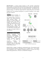
MOSAICS-EM is a software package designed to refine molecular conformations
directly against two-dimensional (2D) electron-microscopy images. By optimizing the
orientation of the projection at the same time as the conformation, it is particularly wellsuited to the 2D class-averages from cryo-electron microscopy. By directly using
projection images, we relieve the urgent need for a density map that is not always
available due to the structural heterogeneity or preferred orientations of the sample
molecules on the grid.
Objective
In our refinement procedure, we
change the atomic coordinates of
the molecular model to increase its
match to the electron-microscopy
(EM) projection images.
In
addition, we locally optimize the
projection angle of the model to
minimize the inaccuracy of the
orientation parameters for the target
image (Fig. 1).
This is done
iteratively with a Monte Carlobased optimization procedure. We
use Natural Moves to greatly reduce
the degrees-of-freedom (DOFs) in
the refinement.
Implementation of MOSAICS-EM
MOSAICS-EM is built upon two
software
programs
called
MOSAICS (Methodologies for
Optimization and SAmpling In
Computational
Studies)
and
EMAN2 (Electron Microscopy
ANalysis 2).
We utilize the
powerful
sampling
and
minimization
methods
in
MOSAICS while the basic image
processing routines are called from
EMAN2 library (Fig. 2).
Figure 1. Refining model conformation and orientation.
Figure 2. Architecture of MOSAICS-EM.
MOSAICS-EM is capable of sampling the conformational space of the molecular model
with much improved efficiency using natural moves at multiple scales. We use Monte
Carlo minimization with a modulated temperature profile to overcome local energy
minima during optimization. (reference to our MOSAICS-EM paper)
2
Installation of MOSAICS-EM
1) EMAN2 is a software package developed by researchers at Baylor College of
Medicine to perform single-particle image processing for electron-microscopy data.
To install EMAN2, you can use one of the two following options:
Option A)
Install EMAN2 by following the procedure at:
http://blake.bcm.edu/emanwiki/EMAN2/Install
Option B)
Precompiled EMAN2 libraries are provided in MOSAICS-EM
2) Download MOSAICS-EM.3.8 source code at:
http://csb.stanford.edu/~minary/mosaics/download.html
3) Untar version.3.8-EM.tar.gz and change the directory into source/compile/serial
4) Edit file Makefile and change the following two lines to your EMAN2 library and
header directories:
INCLEM2 = /EMAN2-header-files-directory/
LIBEM2 = /EMAN2-library-files-directory/
“EMAN2-header-files-directory” is where you put your EMAN2 header files.
“EMAN2-library-files-directory” is where you put your EMAN2 library file. If you
put the EMAN2 header files under /EMAN2/include and EMAN2 library files under
/usr/local/lib, then you specify:
INCLEM2 = /EMAN2/include
LIBEM2 = /usr/local/lib
5) Type “make” and your C++ compiler will compile and make the executable file
“mosaics.x” in the directory called “examples”.
6) Further installation instructions are available at:
http://csb.stanford.edu/~minary/mosaics/install.html
3
Running MOSAICS-EM with lysozyme artificial data
To run a simple MOSAICS-EM refinement, the following files are required:
1) init.pdb
input PDB coordinates of your model
2) refine.input
parameter file that defines global refinement
parameters
3) target.hed &.img
input target EM image
4) orientation.data
parameter file for the target image
5) region.data
region file required if you want to use multi-scale
natural move DOFs.
6) top_3pt_prot_na.rtf
topology file for the molecular model
7) par_3pt_prot_na.prm
potential energy file for the molecular model
These files can be downloaded from link:
http://csb.stanford.edu/~minary/mosaics_em/examples/lysozyme.tar.gz
Unzip this archive and change to its directory.
typing:
Run MOSAICS-EM refinement by
/MOSAICS-EM-directory/mosaics.x refine.input > out
“MOSAICS-EM-directory” is where the mosaics.x file is. The output information of the
refinement is piped to a file called “out”. A file with name sim_param.out will be created
in the current directory in which all the current refinement parameters will be recorded.
You can monitor the temperature of your Monte-Carlo refinement by typing:
cat out | grep Temperature
You can monitor the acceptance-ratio of your Monte-Carlo refinement by typing:
cat out | grep “Chain 0”
You can monitor the EM energy of your Monte-Carlo refinement by typing:
cat out | grep Cryo
4
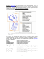
Input PDB file (init.pdb)
In order to use natural move DOFs, a molecular model is represented as segments
connected by flexible loops. Rotational and translational degrees-of-freedom can be
assigned to each segment and a chain-closure algorithm (Minary and Levitt, 2010) is used
to maintain chain connectivity and correct stereochemistry along the connected loop
regions. The cartoon on the left of Fig. 3 is an illustration of how a molecular structure
can be defined as several segments connected by flexible loops.
Figure 3. An illustration of a model represented as 3 rigid segments connected by 2 flexible loops (left) and the first
few lines of its corresponding initial PDB file with the STRIDE record defining segments and loops.
On the right hand side of Fig.3 shows the format of an initial PDB file corresponding to
the model represented on the left. The field CBLC ~A defines there is only one chain A.
If you have more than one chain, such as Chain A and Chain B, you can specify
CBLC ~AB
In the field STRIDE, R means this residue belongs to a segment, C means this residue
belongs to a loop within which the chain-closure needs to be solved. To use the
knowledge-based potential, each macromolecular residue is represented by a 3-point
model that consists of the C!, carbonyl O atoms and a centroid (CMA) for the side
chain. If you have more than one chain, you need to define each STRIDE for each chain.
5
Refinement parameter file (refine.input):
This parameter file is also used in the non-EM version of MOSAICS, which performs
molecular simulation not related to the EM refinement. Some parameters in this file are
not related to the MOSAICS-EM refinement but are still in this file for the completeness
of the input. For complete explanations of all the parameters of the refinement parameter
file, please refer to the MOSAICS user manual at
http://csb.stanford.edu/minary/mosaics/manual.pdf
Here we explain several parameters related to a particular MOSAICS-EM refinement.
The first section of the refine.input file, ~sim_gen_def, defines the necessary parameters
to run the refinement. Below are the basic parameters one may need to adjust for his own
project using MOSAICS-EM.
~sim_gen_def[
\simulation_typ{MIN}
\minimize_type{stsamc}
\prop_tors_sig{0}
\prop_rot_sig{1.e-4}
\prop_trans_sig{1.e-3}
\prop_clos_sig{1.e-3}
\total_step_mc{7000}
\statistics_freq{100}
\write_energy_unit{Ha}
\stsamc_type{trigonom}
\stsamc_period{4000}
\stsamc_ampl{2500}
\stsamc_shift{0}
\random_seed{-9378000501}
……
the simulation type is minimization
temperature-modulated simulated annealing Monte
Calo is used
In each Monte Carlo step, the newly sampled torsion
angle between adjacent atoms in one segment is
chosen from a normal distribution centered around
the original angle with standard deviation, ! defined
by \prop_tors_sig{!}. The larger ! is, the broader
the normal distribution, and the higher the
probability that a larger torsional step size is taken.
Unit is in radians. Here we set it to 0 to make the
segment rigid.
Similar to \prop_tors_sig{}, but for the global
rotation angles of a segment. Unit is in radians. This
is overwritten in the region file if multi-scale natural
move is used.
Similar to \prop_tors_sig{}, but for the global
translation of a segment. Unit is in Å. This is
overwritten in the region file if multi-scale natural
move is used.
Similar to \prop_tors_sig{}, but is used for chainclosure. Unit is in Å.
number of refinement steps
Output results every 100 refinement steps
Unit of the output energy. Ha: atomic unit, kcal:
kcal/mol
type of temperature modulation to use
period for the temperature modulation
amplitude for the temperature modulation
baseline temperature for the temperature modulation
random number to initialize the Monte Carlo
]
6
The second section of refine.input file, ~sim_mol_def, defines the basic parameters of
the model and energy related to the MOSAICS-EM refinement.
~sim_mol_def[
……
\cgres_model{KB_3pt} KB_3pt, off
\mol_parm_file{top_3pt_prot_na.rtf}
\inter_database_file{par_3pt_prot_na.prm}
\cryo_em_database_file{orientation.data}
\pos_init_file{init.pdb}
\pos_out_file{sampled.pdb}
\atom_pos_file{sampled.pos}
\epot_file{sampled.pot_energy}
\einter_file{sampled.inter_energy}
\energy_term{inter}
\energy_term{cryo_em}
use a 3-point coarse-grained model
topology file for the molecule
potential file for the inter energy
parameter file for the target image
initial PDB file
PDB file for the last sampled
conformation
output file for the refinement
trajectory
output file for the sampled potential
energy
output file for the sampled inter
energy
to use the inter energy
to use the EM energy from the
target 2D image
……
]
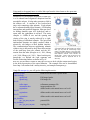
Target image file (target.hed and target.img):
This is the target 2D image that you are refining against.
Class-averages with high signal-to-noise ratio are
usually used. In this example, we use some artificial
data without any noise.
It is in the imagic format
containing one header (target.hed) and one actual image
(target.img). You can view it with any single-particle
EM image viewer, such as the v2 command in EMAN.
7
Figure 4. the target
image viewed with EMAN
command v2.
Image parameter file (orientation.data):
This is an example of the orientation.data file, which defines all the necessary parameters
of the input target image.
~cryo_em_parm[\pot_type{normal}[\ea_az {0}\ea_alt{0}\ea_phi{0}
\ea_range{0}\ea_interval{5}
\pixel_size{2}\resol_blur{10}
\expermnt_file{target.hed}
\energy_scale{5}
]
Below are the parameters that need to be modified for one particular image.
\ea_az{}
initial azimuthal angle for the model projection (unit in degree)
\ea_alt{}
initial altitude angle for the model projection (unit in degree)
\ea_phi{}
initial phi angle for the model projection (unit in degree)
\ea_range{}
range to locally sample the around the current Euler angles (unit in
degree)
\ea_interval{}
interval for the local variation of the Euler angles (az, alt, phi) (unit
in degree)
\pixel_size{}
pixel size of the target image (unit in Å/pixel)
\resol_blur{}
resolution to blur the model to match the target image (unit in Å)
\expermnt_file{}
path to the target image
\energy_scale{}
weight for the EM energy
In the above example, we set \ea_range{0} so no local optimization of the projection
Euler angle is performed. We can also introduce wrong initial Euler angle parameters
and then let MOSAICS-EM to refine the Euler angles as in the file orientation2.data.
~cryo_em_parm[\pot_type{normal}[\ea_az {0}\ea_alt{8}\ea_phi{0}
\ea_range{2}\ea_interval{1}
……
]
In orientation2.data file, we introduce an altitude deviation of 8 degrees. We then let
MOSAICS-EM to optimize the Euler angles around the current ones between ±2 degrees
with an interval of 1 degree.
You can then run the refinement for both conformation and orientation by typing:
/MOSAICS-EM-directory/mosaics.x refine-euler.input > out
If you have more than one target images, an image parameter file can contain multiple
~cryo_em_parm[…] records with each one defines the parameters of its corresponding
target 2D image. This provides more experimental structural information since
projections of more than one viewing angle are used. But only use this option when the
conformations captured by these images are identical.
8
Region file (region.data): This representation was first introduced in the context of
sampling by hierarchical natural moves (Sim et al., 2012), where the region elements
were residues. Here, we further develop this technology to include segments as region
elements and use it in our multi-scale natural move refinement.
The multi-scale natural moves are defined in this region file.
Figure 5. An illustration of the customization of two regions (left) and their corresponding definitions (right) in
the region.data file.
Fig. 5 shows how the multi-scale natural moves can be used by defining regions
consisting of different segments. Each region is assigned the independent degrees-offreedom. On the right hand side of Fig. 5 are examples of the regions in the region.data
file with the parameters:
\nseg{}
number of segments in a region
\ncenter{}
number of rotational center in a region
\segments_firstres{}
the first residue for each segment
\segments_lastres{}
the last residue in each segment
\segments_baseres{}
the middle residue in each segment
\centers{}
the residue used as the rotational centers for this region. It
can be either 1 or any of the residues defined in
\segments_baseres
\prop_trans_sig{}
overwrite \prop_trans_sig{} in refinement parameter file to
define its value for each region
\prop_rot_sig{}
overwrite \prop_rot_sig{} in refinement parameter file to
define its value for each region
9
\prop_trans_sig_freeres{}
\prop_rot_sig_freeres{}
similar to \prop_trans_sig{} but for each segments within a
region (unit in Å). Set it to zero if no movement is allowed
between each segment in a region.
similar to \prop_rot_sig{} but for each segments within a
region (unit in radians). Set it to zero if no movement is
allowed between each segments in a region.
The refinement parameter file also needs to be revised accordingly to use the region file.
One line is added in the ~/sim_mol_def section:
\region_database_file{region.data}
Please see the file refine-region.input. You can then run the refinement with multi-scale
natural moves by typing:
/MOSAICS-EM-directory/mosaics.x refine-region.input > out
This example shows how multi-scale natural move can be used. But little is gained by
performing it on a small molecule, such as the lysozyme. In the next example, we will
demonstrate how multi-scale natural moves can be used to greatly facilitate the
refinement on a large macromolecular complex, the Methonococcus maripaludis
chaperonin, or Mm-cpn, against a real experimental 2D cryo-EM class-average.
10
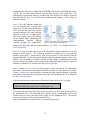
Using multi-scale natural move to refine Mm-cpn from the closed state to the open state
with a single cryo-EM class-average.
Methonococcus maripaludis chaperonin, or Mm-cpn,
A
B
is a 16-subunit homo-oligomeric chaperon from the
mesophilic archaea. It helps other proteins to fold in
the archaea cell. It consists of two back-to-back
rings each containing eight subunits. Each subunit
has a substrate-binding apical domain, ATP-binding
C
intermediate and equatorial domains. Mm-cpn closes
its folding chamber upon ATP hydrolysis and reopens after the "-phosphate is released. The entire
complex is ~1MDa in size and the opening and
closing of the ring is mostly achieved by a rigidbody rocking of individual subunits. The apical and
intermediate domains are tightly coupled within a
subunit by salt bridges at their domain interface.
The communication between neighboring subunits
Figure 6. (A) top view (left) and side view (left)
of the lidless Mm-cpn initial model in the closed
within a ring is delivered by the #-sheet that consists
state. (B) top view 2D class-average target
of the stem-loop from one subunit and the NCimage of the lidless Mm-cpn in the open state.
(C) segments and connections as illustrated with
termini from the other (Douglas et al., 2011; Zhang
three adjacent subunits. Three subunits are
et al., 2010; Zhang et al., 2011). Based on this prior
labeled with I, ii and iii. API for apical, INT for
intermediate, EQU for equatorial and SL for
knowledge, we defined the rigid segments and
stem-loop.
flexible connecting linkers as shown in Fig. 6C.
Here we use the lidless variant of Mm-cpn so as not to deal with the unstructured region
in the helical protrusion of the apical domains. The example files can be downloaded
from: http://csb.stanford.edu/~minary/mosaics_em/examples/mmcpn.tar.gz
Unzip file mmcpn.zip, you will get the following directories:
lidless-3pt.pdb
class-average:
open.0.hed
open.0.img
level1:
refine.input
orientation.data
region.data
level2:
region.data
level3:
region.data
pot_database:
par_3pt_prot_na.prm
top_database:
par_3pt_prot_na.prm
PDB file for the initial 3-point model
EM image header
EM image file
refinement parameter file
image parameter file
defines multi-scale natural moves at level 1
defines multi-scale natural moves at level 2
defines multi-scale natural moves at level 3
potential file
topology file
11
Segments of the Mm-cpn are defined in the STRIDE record of the initial PDB file lidless3pt.pdb. We can then group different segments into regions in the region files. We
subsequently represent the Mm-cpn model using more numbers of smaller regions at
hierarchical levels (Fig. 7) to describe finer conformational changes. These levels are
defined as follows:
Level 1: All the segments within the
box are grouped into a single rigid
region in a way that chain breaks may
occur between the stem-loop and the
equatorial domain. The entire Mm-cpn
complex is treated as 16 rigid regions.
This level captures the overall rocking
of the subunit while maintaining the
communication
between
adjacent
Figure 7. Three levels of region compositions for a single
subunit with hierarchically increasing DOFs.
subunits through the “hand-shake”
between the stem-loop and NC-termini (Zhang et al., 2010). It is defined in the file
level1/region.data.
Level 2: In each Mm-cpn subunit, apical & intermediate domain segments in one box
belong to rigid region 1. The remaining segments in another box are grouped into
another rigid region 2. Chain-closures may occur between: (a) the stem-loop and the
equatorial domain; (b) the intermediate domain and the equatorial domain of the same
subunit. The entire Mm-cpn complex contains 32 rigid regions. In addition to the overall
subunit rocking, the relative motion between the equatorial domain and the other two
domains are allowed. It is defined in the file level2/region.data.
Level 3: Based on Level 2, now we divide region 2 into 4 sub-regions. All sub-regions
have their own rotational and translational DOFs and they are kept connected by chainclosures. At this level, more flexibility is introduced in the equatorial domain to describe
more subtle conformational fluctuations around the ATP-binding pocket. It is defined in
the file level3/region.data.
You can run multi-scale natural move refinement of Mm-cpn at level 1 by typing:
cd level1
/MOSAICS-EM-directory/mosaics.x refine.input > out
The model with the lowest EM energy at the current level is used as the initial model for
the subsequent level. The optimized Euler angles for that corresponding model at the
current level are used as the initial Euler angles for the subsequent level. We provide
some useful scripts, which can be downloaded from:
http://csb.stanford.edu/~minary/mosaics_em/scripts/scripts.tar.gz
12
References:
(1) Douglas, N.R., Reissmann, S., Zhang, J., Chen, B., Jakana, J., Kumar, R., Chiu, W., and
Frydman, J. (2011). Dual action of ATP hydrolysis couples lid closure to substrate
release into the group II chaperonin chamber. Cell 144, 240-252.
(2) Minary, P., and Levitt, M. (2010). Conformational optimization with natural degrees of
freedom: a novel stochastic chain closure algorithm. J Comput Biol 17, 993-1010.
(3) Sim, AYL, Levitt, M., and Minary, P. (2012) Modeling and design by hierarchical natural
moves. Proc. Natl. Acad Sci U S A In press.
(4) Zhang, J., Baker, M.L., Schroder, G.F., Douglas, N.R., Reissmann, S., Jakana, J.,
Dougherty, M., Fu, C.J., Levitt, M., Ludtke, S.J., et al. (2010). Mechanism of folding
chamber closure in a group II chaperonin. Nature 463, 379-383.
(5) Zhang, J., Ma, B., DiMaio, F., Douglas, N.R., Joachimiak, L.A., Baker, D., Frydman, J.,
Levitt, M., and Chiu, W. (2011). Cryo-EM structure of a group II chaperonin in the
prehydrolysis ATP-bound state leading to lid closure. Structure 19, 633-639.
13