Download Bachelor Thesis - Fachbereich Informatik

Fachhochschule
Bonn-Rhein-Sieg
University of Applied Sciences
Fachbereich Informatik
Department of Computer Science
Bachelor Thesis
Integration of Physical and Psychological Stress Factors
into a VR-based Simulation Environment
by
David Scherfgen
First examiner:
Prof. Dr. Rainer Herpers
Second examiner: Prof. Dr. Dietmar Reinert
Handed in on:
16th of October, 2008
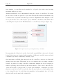
Acknowledgements
Page i
Acknowledgements
I would like to thank my examiners Prof. Dr. Rainer Herpers and Prof. Dr. Dietmar
Reinert as well as the whole FIVIS project team for their support and for giving me
the opportunity to write my thesis within the context of this interesting and challenging project.
My thanks are due to Evangelos Zotos and Holger Steiner for their valuable assistance with the testing of the developed software. I would also like to thank Michael
Kutz for his advices and for encouraging me to write this thesis.
The FIVIS bicycle sensor system was developed by Christian Zimmermann, Nico Ziegenhals and Philipp Müller-Leven. Thank you very much for your commitment!
Finally, I would like to thank my family and my friends for their support and understanding.
Abstract
Page iii
Abstract
The “FIVIS” project (Fahrradsimulation in der immersiven Visualisierungsumgebung
“Immersion Square” – bicycle simulation in the immersive visualization environment
“Immersion Square”) at the Bonn-Rhein-Sieg University of Applied Sciences aims at
creating an immersive low-cost PC-based bicycle simulator using a three-screen rear
projection system and a sensor-equipped bicycle mounted on a motion platform.
This thesis approaches the problem of developing an expandable bicycle simulation
software solution for FIVIS. This includes simulating and visualizing a virtual world
that the user can interact with using the bicycle. Employing the simulator as a
framework, a concrete scenario is developed that exposes the bicycle rider to scalable
physical and psychological strains, as required for stress-related research projects
conducted by the BGIA Institute for Occupational Safety and Health.
A layered simulation model is designed and implemented that performs the simulation and interaction of virtual objects at different abstraction levels. The visualization
is based on a well proven 3D engine and features a flexible rendering approach that
generates perspective-correct images for screens of arbitrary number and alignment in
space, while taking the user’s head position into account. Bicycle dynamics and physical object interactions are modeled using a physics engine. The virtual bicycle can be
controlled using the sensor-equipped bicycle provided by the FIVIS project. Expandability is achieved by implementing a scripting interface.
Scalable physical and psychological stress factors suitable for the bicycle simulation
are identified and implemented. Simulation events are logged in a way that makes
them easily accessible for further evaluation.
First tests have been conducted within the context of road safety education and the
stress generation, with promising results.
Statement of originality
Page v
Statement of originality
I hereby declare that this thesis is my own work and has not been submitted in any
form for another degree at any university or other institute of tertiary education. Information derived from the published and unpublished work of others has been acknowledged in the text and a list of references is given in the bibliography.
Hiermit erkläre ich, dass ich die vorliegende Bachelor-Arbeit selbständig angefertigt
habe. Es wurden nur die in der Arbeit ausdrücklich benannten Quellen und
Hilfsmittel benutzt. Wörtlich oder sinngemäß übernommenes Gedankengut habe ich
als solches kenntlich gemacht.
Sankt Augustin, 16th of October, 2008
.
(David Scherfgen)
Table of contents
Page vii
Table of contents
Acknowledgements ...................................................................................... i
Abstract ..................................................................................................... iii
Statement of originality .............................................................................. v
Table of contents ...................................................................................... vii
Figures ....................................................................................................... xi
Tables ...................................................................................................... xiii
Listings .................................................................................................... xiv
1
2
3
Introduction.......................................................................................... 1
1.1
Thesis outline.............................................................................................. 1
1.2
Background and motivation........................................................................ 2
1.3
Platform...................................................................................................... 3
1.4
Areas of application .................................................................................... 5
1.5
BGIA survey ............................................................................................... 5
1.6
Related work............................................................................................... 6
1.6.1
FIVIS simulator software prototype ................................................ 6
1.6.2
OpenGL wrapper for the Immersion Square ................................... 7
1.6.3
Bicycle dynamics ............................................................................. 7
1.6.4
Immersion, presence and training effects ......................................... 7
1.6.5
Presence in virtual environments .................................................... 8
1.6.6
Other simulators ............................................................................. 8
1.7
Problems to be solved ................................................................................. 9
1.8
Terminology................................................................................................ 9
1.9
Mathematical notation.............................................................................. 10
Problem discussion ............................................................................. 11
2.1
Immersion ................................................................................................. 11
2.2
Simulation approach ................................................................................. 11
2.3
Platform.................................................................................................... 12
2.4
Flexibility ................................................................................................. 13
2.5
Stress factor survey ................................................................................... 13
Methods and tools .............................................................................. 15
3.1
Scripting language .................................................................................... 15
3.2
3D graphics ............................................................................................... 15
3.3
3D audio ................................................................................................... 17
Page viii
3.4
3.5
4
Physics simulation..................................................................................... 18
3.4.1
Rigid bodies ................................................................................... 18
3.4.2
Shapes and materials ..................................................................... 19
3.4.3
Joints ............................................................................................. 20
3.4.4
Discrete time steps ........................................................................ 20
3.4.5
Potential problems......................................................................... 21
Bicycle dynamics ....................................................................................... 22
3.5.1
Self-stability and geometric properties........................................... 22
3.5.2
Turning, steering, leaning and forces ............................................. 23
Approach............................................................................................. 27
4.1
Layered simulation model ......................................................................... 27
4.1.1
Physical layer ................................................................................ 28
4.1.2
Logical layer .................................................................................. 28
4.1.3
Control layer ................................................................................. 29
4.1.4
Semantic layer ............................................................................... 31
4.2
World concept ........................................................................................... 31
4.3
Expandability ............................................................................................ 32
4.4
4.5
5
Table of contents
4.3.1
Factories ........................................................................................ 32
4.3.2
Events ........................................................................................... 32
4.3.3
Data representation ....................................................................... 32
Bicycle model ............................................................................................ 34
4.4.1
Rigid body setup ........................................................................... 34
4.4.2
Steering and lean angle.................................................................. 36
4.4.3
Head wind sound ........................................................................... 38
Visualization ............................................................................................. 38
4.5.1
Camera object ............................................................................... 38
4.5.2
Simple rendering approaches ......................................................... 39
4.5.3
Advanced rendering approach ....................................................... 41
4.5.4
Depth perception ........................................................................... 45
4.6
Simulation loop ......................................................................................... 46
4.7
FIVIStress application............................................................................... 47
4.7.1
Physical stress ............................................................................... 47
4.7.2
Emotional stress ............................................................................ 48
4.7.3
Controlling the simulation ............................................................. 50
4.7.4
Data logging .................................................................................. 51
Realization .......................................................................................... 53
Table of contents
5.1
5.2
Languages and libraries used .................................................................... 53
5.1.1
Programming language: C++ ....................................................... 53
5.1.2
Scripting language: Python ........................................................... 55
5.1.3
3D graphics engine: Ogre3D .......................................................... 56
5.1.4
3D audio engine: FMOD ............................................................... 59
5.1.5
Physics engine: PhysX .................................................................. 60
5.1.6
XML parser: TinyXML ................................................................. 61
Simulation layer implementation .............................................................. 61
5.2.1
Objects .......................................................................................... 61
5.2.2
Controllers .................................................................................... 64
5.2.3
Python for the semantic layer ....................................................... 65
5.3
World objects............................................................................................ 65
5.4
Simulator object........................................................................................ 66
5.5
Adjusting the cameras .............................................................................. 67
5.6
Python interface ....................................................................................... 68
5.7
Bicycle object ............................................................................................ 70
5.8
Hardware bicycle controller ...................................................................... 70
5.9
6
Page ix
5.8.1
Data protocol ................................................................................ 70
5.8.2
Implementation ............................................................................. 71
FIVIStress application .............................................................................. 72
5.9.1
City model .................................................................................... 72
5.9.2
Stress parameters .......................................................................... 73
5.9.3
Applying the pedal factor.............................................................. 74
5.9.4
Checkpoints................................................................................... 74
5.9.5
Cars............................................................................................... 75
5.9.6
Boxes ............................................................................................ 76
5.9.7
Status sample logging and screenshots .......................................... 77
5.9.8
Remote console ............................................................................. 78
Results and evaluation........................................................................ 81
6.1
Visualization ............................................................................................. 81
6.2
Physics ...................................................................................................... 82
6.3
Expandability ........................................................................................... 83
6.4
Road safety education test ........................................................................ 83
6.5
6.4.1
Subjects and procedure ................................................................. 83
6.4.2
Results .......................................................................................... 86
FIVIStress test .......................................................................................... 87
Page x
7
Table of contents
6.5.1
Subject and procedure ................................................................... 87
6.5.2
Results ........................................................................................... 87
Conclusion and future work ................................................................ 93
7.1
Summary ................................................................................................... 93
7.2
Future improvements ................................................................................ 93
7.3
7.2.1
Extending FIVIStress .................................................................... 94
7.2.2
Rendering large scenes ................................................................... 94
7.2.3
Improved bicycle physics ............................................................... 94
7.2.4
More powerful Python interface .................................................... 95
7.2.5
World editor .................................................................................. 95
Proposals for FIVIS................................................................................... 95
7.3.1
Solving the braking problem.......................................................... 95
7.3.2
Head tracking ................................................................................ 96
7.3.3
Making the shoulder check possible ............................................... 96
7.3.4
Wind ............................................................................................. 96
Bibliography.............................................................................................. 97
CD contents .............................................................................................. 99
Figures
Page xi
Figures
Figure 1-1: Concept of an interactive vehicle simulator ............................................... 2
Figure 1-2: Concept rendering of the FIVIS system in an advanced configuration ...... 4
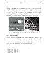
Figure 1-3: FIVIS on the Hannover Messe (photograph by Thorsten Hümpel) ........... 6
Figure 3-1: Scene graph representation of a tank....................................................... 17
Figure 3-2: Selected geometric properties of a bicycle................................................ 23
Figure 3-3: Forces acting upon the bicycle while turning .......................................... 24
Figure 4-1: Physical layer view of bicycle sub-objects................................................ 28
Figure 4-2: Logical bicycle providing steering and acceleration functionality ............ 29
Figure 4-3: Logical bicycle object being affected by controllers ................................. 30
Figure 4-4: Physical bicycle model ............................................................................. 35
Figure 4-5: Determining the curve radius .................................................................. 37
Figure 4-6: Top view of the FIVISquare .................................................................... 39
Figure 4-7: Single wide-angle rendering, limited to 180° ............................................ 40
Figure 4-8: Three separate renderings combined, not limited to 180° ........................ 40
Figure 4-9: Screen as a window into the virtual world .............................................. 41
Figure 4-10: Explanation of the viewing frustum parameters .................................... 43
Figure 4-11: Explanation of screen representation parameters................................... 44
Figure 4-12: Displaying the correct image on each projection screen ......................... 44
Figure 4-13: Example scene with five checkpoints ..................................................... 49
Figure 4-14: Cars approaching the user’s bicycle have to be evaded ......................... 49
Figure 5-1: Overview of Ogre3D classes used by FIVISim ......................................... 58
Figure 5-2: Object managing its controllers and its sub-objects representations........ 62
Figure 5-3: Simulator acting as manager for factories and resources ......................... 66
Figure 5-4: Updating the hardware bicycle controller ................................................ 72
Figure 5-5: Visual mesh, physical mesh and texture of a building ............................. 73
Figure 5-6: 3D representations of the checkpoint objects’ countdown numbers ......... 74
Figure 5-7: Updating checkpoint objects.................................................................... 75
Figure 5-8: 3D mesh used for the cars (“Yugo” model from turbosquid.com) ............ 76
Figure 5-9: Processing remote commands on the server............................................. 79
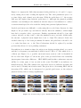
Figure 6-1: Screenshots taken from FIVIStress .......................................................... 82
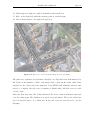
Figure 6-2: Test route overview (satellite image from Google Earth) ........................ 85
Figure 6-3: FIVIStress proband with CUELA sensors riding the FIVIS bicycle ........ 88
Page xii
Figures
Figure 6-4: Sensor data and skeleton visualization in WIDAAN................................ 88
Figure 6-5: Stressful riding sequence (FIVIStress screenshots) ................................... 89
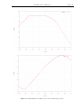
Figure 6-6: PAI plots for pedal factor 1 and 1.5 ........................................................ 90
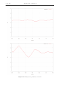
Figure 6-7: HRV:MSSD and SCR plots for the stressful riding sequence ................... 91
Tables
Page xiii
Tables
Table 1-1: Mathematical notation used in this work ................................................. 10
Table 3-1: Translational and rotational quantities of rigid bodies ............................. 19
Table 4-1: Overview of FIVIStress parameters .......................................................... 50
Table 5-1: Built-in object types ................................................................................. 63
Table 5-2: Built-in controller types............................................................................ 65
Table 6-1: Test route results...................................................................................... 86
Page xiv
Listings
Listings
Listing 4-1: Example world XML description............................................................. 33
Listing 5-1: Simple Python example program ............................................................ 55
Listing 5-2: Simple C++ example program................................................................ 56
Listing 5-3: A simple Python program using FIVISim ............................................... 69
Listing 5-4: Structures for UDP packets from the hardware to the software ............. 71
Listing 5-5: Stress parameter initialization ................................................................. 73
Listing 5-6: Finding and manipulating the hardware bicycle controller ..................... 74
Listing 5-7: Dynamic creation of boxes ...................................................................... 76
Listing 5-8: Status sample logging and taking of screenshots ..................................... 77
Listing 5-9: Simple remote console for FIVIStress ...................................................... 79
Introduction
1
Page 1
Introduction
FIVIS is a project conducted by the Bonn-Rhein-Sieg University of Applied Sciences
in Sankt Augustin, Germany, in cooperation with the RheinAhrCampus (Koblenz
University of Applied Sciences) in Remagen, Germany. It aims to realize an immersive and realistic low-cost bicycle riding simulation capable of simulating urban environments including autonomously controlled vehicles and pedestrians [1].
In this thesis, the simulation software for FIVIS has to be developed. As a concrete
application, a scenario has to be designed and implemented that exposes the bicycle
rider to scalable strains. This stress factor scenario will later be used by the BGIA
Institute for Occupational Safety and Health within the context of research projects
assessing combined physical and psychological stress factors [2].
1.1 Thesis outline
This thesis is divided into seven chapters. Chapter one first provides a primer on the
topic of vehicle simulators and introduces the FIVIS project. Related work, such as
other simulators, are briefly presented at the end of the chapter.
Chapter two discusses the problems this thesis will have to solve. For example, an
adequate physical bicycle model will have to be found. Methods and tools lending
themselves to be used in a vehicle simulation are introduced in chapter three. These
are 3D graphics, physics simulation and the use of a scripting language. A solution
approach for the problems discussed in chapter two is developed in chapter four, using the tools and methods from chapter three. A layered simulation model is proposed, along with a visualization technique that allows perspective-correct rendering
to arbitrarily aligned screens and takes the user’s head position into account. Chapter
five describes the actual realization of the simulation software and the stress factor
scenario with concrete programming languages and libraries.
An evaluation of the developed software applications follows in chapter six. Finally,
chapter seven concludes and makes some proposals about what could be further improved or extended in the future.
Page 2
Introduction
1.2 Background and motivation
Realistic interactive simulators exist for most types of vehicles, for example airplanes,
helicopters, trains, tanks or cars.
Usually, the cockpit, relevant instruments and controls are built as real components.
The inputs made by the user are then fed into the simulation software that computes
a more or less complete simulation model of the vehicle and its environment. As the
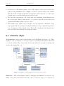
software calculates the new model state depending on the user’s actions and the simulation rules, feedback is given by updating the 3D visualization and the instruments or playing sounds. The user then interprets the simulator output and responds
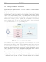
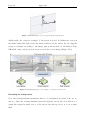
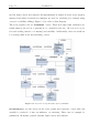
to it again. This simulation loop is depicted in Figure 1-1.
Figure 1-1: Concept of an interactive vehicle simulator
The visualization may be realized by projecting the rendered images onto a screen
that surrounds the vehicle mock-up. Advanced simulators can also move and rotate
the vehicle within certain limits (for example using a Stewart platform) in order to
increase the immersion and provide the user with feedback concerning his motion.
This is comparable to rides found in amusement parks. But unlike those, an interactive simulator has to react to user inputs and respond in real-time.
The use of vehicle simulators is motivated by two main reasons:

Costs: Using a simulator is cheaper than using real vehicles because of fuel and
maintenance work, especially for complex vehicles like airplanes. Also, the simula-
Introduction
Page 3
tor itself is often cheaper than a real vehicle. Sometimes, the vehicle to be tested
doesn’t even exist yet. In this case, it is not necessary to manufacture an expensive early prototype, as it can be simulated.

Safety: Emergency situations that need to be trained would expose both the
driver and the instructor to great danger. In contrast, a simulator provides a safe,
controllable environment that can confront the user with any situation instantly,
without losing valuable time.
However, bicycle simulators are rare. One reason may be the unfavorable relation
between the costs of a real bicycle and the costs of building a simulator. Also, learning to ride a bicycle is not comparable to learning to fly an airplane or to conduct a
train. Therefore, bicycle simulator products don’t seem to be as economically profitable as airplane or car simulators.
A bicycle simulator could serve as a framework for many scientific research projects.
For example, it would be a valuable tool for performing combined physical and psychological studies, since the bicycle differs from all the other vehicles listed above in
one point: It requires the rider to exert manual work.
1.3 Platform
The immersive visualization environment “FIVISquare” consists of three screens (dnp
Alpha Screen), angled by 120°, on which computer-generated images are projected by
three SXGA projectors using rear projection with mirrors. The screens are 1361 mm
× 1021 mm each and cover a huge fraction of the rider’s visual field, including the
peripheral part, which can help create a remarkable immersive effect.
A single standard PC (Intel Core 2 Duo with 4 GB of RAM) equipped with a powerful graphics card (NVIDIA Quadro FX 4500 X2) performs the actual simulation and
renders the images. This is made possible by Matrox’ TripleHead2Go technology 1,
which allows to connect up to three displays to a single VGA or DVI output, providing a maximum combined resolution of 3840×1024 pixels.
1
http://www.matrox.com/graphics/en/products/gxm/th2go/
Page 4
Introduction
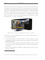
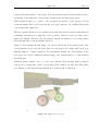
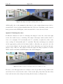
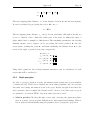
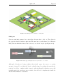
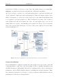
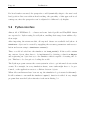
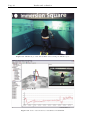
The rider is seated on a bicycle located in front of the three screens (see Figure 1-2).
It is equipped with a potentiometer-based sensor measuring the current steering angle
and an electro-optical sensor measuring the current rotational speed of the bicycle’s
back wheel. At the moment, the back wheel is attached to a Tacx Cycletrainer 2,
which exerts a manually adjustable level of resistance. The sensor output is processed
by a microcontroller unit at 25 Hz and then sent to the simulation PC via UDP.
When receiving the processed sensor data, the simulation software will have to adjust
the virtual bicycle to conform to the real bicycle.
Figure 1-2: Concept rendering of the FIVIS system in an advanced configuration
At the time of writing, the FIVIS system is not yet completely built. Planned, but
not yet finished parts include:

A motion platform that the bicycle is mounted on in order to simulate forces and
the properties of different ground types (the motion platform is developed at the
RheinAhrCampus) [3].

An active motor brake acting upon the back wheel, making it possible to require
the rider to pedal harder when riding uphill and to accelerate the wheel when rolling downhill.

Sensors for measuring the rider’s shifting of weight, since this can also be used for
balancing and steering.
2
http://www.tacx.com/producten.php?language=EN&lvlMain=16&lvlSub=57&ttop=Cycletrainers
Introduction
Page 5
1.4 Areas of application
The FIVIS bicycle simulator’s purpose is not to teach how to ride a bicycle, as it is
very difficult to simulate the complete dynamics of bicycle riding and move the real
bicycle realistically enough to make this possible. In opposite, the simulator is mainly
regarded as a platform for scientific research. Possible applications may be:

Studying the psychological effects of artificially altered correlation between the
rider’s physically correct speed and the displayed virtual speed.

Road safety education for children living in metropolitan areas, where it is too
dangerous to do it on the real roads, or for training in advance.

More effective and motivating training for professional bikers.

Investigating the impacts of combined physical and psychological stress factors
(especially by simulating urban environments with traffic). This is the specific application that will be implemented in this thesis.
1.5 BGIA survey
The BGIA is developing a measurement system for monitoring and analyzing workrelated stress. The CUELA system (Computer-unterstützte Erfassung und LangzeitAnalyse von Belastungen des Muskel-Skelett-Systems – computer-supported longtime analysis of strains of the musculoskeletal system) is a sensor suit worn over the
working clothes. It consists of numerous sensors measuring foot pressure, back torsion
and the angle of hip and knee joints and the spine [2].
Additional sensors have been developed for measuring psychological stress by evaluating the user’s electrocardiogram, respiration, skin conductance and blood oxygen saturation. With the CUELA system, physical and psychological strains at workplaces
can be measured, in order to optimize working environments and reduce accident
rates.
The cooperation with the FIVIS project arose from the need of a controllable way for
generating separate physical and psychological stress factors (emotional stress in particular, as opposed to mental stress) in a safe environment. The bicycle simulation
seems to be an appropriate framework for this, as stress can be generated by requiring the rider to pedal and pay attention to the virtual environment.
Page 6
Introduction
1.6 Related work
This section will describe a previously developed prototype of the FIVIS simulation
software and a wrapper for OpenGL that enables rendering to the three screens of the
Immersion Square with any 3D application that uses OpenGL. Also, some other simulators are presented briefly.
1.6.1
FIVIS simulator software prototype
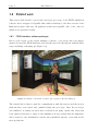
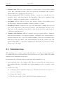
Before work began on the actual simulator software, a prototype has been implemented. It uses the FIVIS hardware and lets the user ride through an artificial landscape, including a ski-jump (see Figure 1-3).
Figure 1-3: FIVIS on the Hannover Messe (photograph by Thorsten Hümpel)
The virtual bike’s behavior and the communication with the sensors and the motion
platform have been tested and optimized using the prototype. Since the prototype
was exhibited on numerous trade fairs, feedback from many casual bike riders has
been gathered and used to improve the simulation. It was evident that the immersive
effect caused by the visualization system was remarkable already, even without the
motion platform.
Introduction
1.6.2
Page 7
OpenGL wrapper for the Immersion Square
The Immersion Square, also developed by the Bonn-Rhein-Sieg University of Applied
Sciences, is a 3D visualization environment with three screens, very similar to the
FIVISquare [4].
When running standard 3D applications in the Immersion Square or the FIVISquare,
the three screens are treated as one single wide screen. But since the screens are actually angled (90° to 135° in the Immersion Square), the perspective in the rendered
image is not correct. Noticeable bends at the screen edges are the result. In order to
render a correct image, each screen has to be rendered independently using an adjusted camera transformation. Standard applications usually don’t do that, as they
haven’t been designed with visualization systems like the Immersion Square in mind.
In order to address this problem, an OpenGL wrapper for Microsoft Windows has
been developed that transparently replaces the standard OpenGL implementation [5].
It intercepts and manipulates the drawing API calls so that the scene is rendered to
all three screens, using the correct perspective. 3 Additionally, the OpenGL wrapper
supports stereoscopic rendering using anaglyphs. The technique for perspectivecorrect rendering to angled screens, which (in a modified form) is also used in the
FIVIS simulation software, is described in chapter four.
1.6.3
Bicycle dynamics
The dynamics of bicycle riding have been analyzed by Franke et al. [6] and Fajans
[7]. Models for describing self stabilization and the relation between the steering angle
and the lean angle are presented. These can be used to make the bicycle simulation
realistic and prevent the virtual bicycle from tilting over.
1.6.4
Immersion, presence and training effects
Bowman and McCahan distinguish between immersion and presence [8]. According to
their work, immersion is an objectively measurable quality of a virtual reality system.
The algorithm used in the OpenGL wrapper actually doesn’t provide perfectly correct images, since it
only shifts and rotates the cameras. In fact, asymmetric viewing frustums have to be used. This will be
accomplished in this thesis.
3
Page 8
Introduction
It depends solely on the quality of computer-generated sensory stimuli, such as 3D
visualization (display size, resolution, field of view, lighting, frame rate and physical
realism), sound and tactile impulses. Presence, on the other hand, is the user’s subjective perception of the virtual reality, the feeling of “being there”. It is affected by
the virtual reality system’s level of immersion, but also by the user’s state of mind
and experience with such systems.
According to Bowman and McCahan, the effectiveness of a virtual reality application
in terms of achieving training effects for the real world largely depend on the user’s
presence in the virtual environment. Therefore, reaching presence through immersion
should be a primary goal for the FIVIS bicycle simulator.
1.6.5
Presence in virtual environments
Meehan et al. predicted that a high level of presence in a virtual environment would
evoke physiological responses similar to those evoked by an equivalent real environment [9]. They developed an approach for a reliable physiological measure of presence. This measure includes the change in heart rate, skin temperature and skin conductance. In their experiment, they were able to generate the expected physiological
responses to a certain degree. One interesting result was that achieving higher visualization frame rates leads to higher presence.
1.6.6
Other simulators
Kwon et al. developed a sophisticated interactive bicycle simulator called KAIST [10].
It features a bicycle mounted on a Stewart platform. The handle and pedaling resistances can be controlled by the simulation, and the pedals can also be actively accelerated using a servo. The bicycle dynamics are computed explicitly, not using a physics engine. However, KAIST needs three simulation computers and does not feature
panoramic rendering.
An immersive vehicle simulator that doesn’t require any mock-ups of the vehicle’s
interiors is presented by Marcelo Kallmann [11]. All input is made via data gloves.
The simulation software uses the Python scripting language to set up scenarios and
control dynamic objects. The concept of using a scripting language for high-level logic
is a reasonable choice that will also be applied in this thesis.
Introduction
Page 9
1.7 Problems to be solved
In order to reach the goal of creating an immersive, realistic bicycle simulation for
the FIVIS project, a simulation model has to be found first. It needs to provide an
adequate degree of physical realism and has to be computable in real-time using a
standard PC. Obviously, some approximations and trade-offs will have to be accepted.
Furthermore, a real-time visualization approach must be found that utilizes the possibilities the FIVISquare offers in order to create an immersive effect for the rider.
The visual quality of the computer-generated images should be as good as possible.
The rendered images should occupy the whole projection screen area and cope with
the fact that the screens are angled.
The actual implementation should be both fast and flexible in order for the simulator
to be usable for a wide range of possibly different scenarios.
Means have to be developed for exposing the bicycle rider to separately scalable
amounts of physical and emotional stress factors.
Finally, the quality and the expandability of the implementation have to be evaluated using reasonable tests.
1.8 Terminology
Throughout the remaining parts of this thesis, the following terms will be used for
the complete simulator system, the simulation software and the stress factor application:

FIVIS system describes the whole physical simulator system, consisting of the
sensor-equipped bicycle, the simulation PC and the projectors and screens.

FIVISim is the name for the simulation software that is developed within the
context of this thesis, including the visualization, sensor input processing and
physical simulation.

FIVIStress is the stress factor scenario that is developed as an application for
FIVISim.
Page 10
Introduction
1.9 Mathematical notation
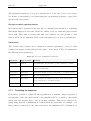
The following mathematical notation will be used in this work:
Table 1-1: Mathematical notation used in this work
Notation
Meaning
v
Vector variable
a ⋅b
Dot product of a and b
a×b
Cross product (vector product) of a and b
v
Magnitude (length) of vector v
v
Vector v normalized (divided by its magnitude)
P
Point in space (treated like a vector)

AB
Vector from point A to point B
Problem discussion
2
Page 11
Problem discussion
An immersive bicycle simulation shall be developed that runs on the FIVIS hardware.
It is planned to be used for several research projects. One of these projects needs to
expose the bicycle rider to independently scalable amounts of physical and emotional
stress factors. It is also planned to be used for road safety training for children, including traffic simulation.
This brief task description contains a number of sub-problems that have to be solved
and requirements to be met. These will be discussed in this chapter.
2.1 Immersion
For the FIVISim software, the results of Bowman [8] and Meehan [9] mean that attention will need to be turned to the task of rendering and animating the images in
order to reach a high level of immersion, which in turn helps to increase the rider’s
presence, create depth perception and allow for training effects that can be applied to
the real world.
A trade-off will have to be found between visual quality and the achievable frame
rate. Also, an approach will be needed for rendering the images in the correct panoramic perspective. The algorithm should produce a correct perspective for both small
and tall users (children and adults). When the motion platform is fully integrated
into the simulator, the user’s head will move around significantly. This should be
compensated so that the user always sees a correct image.
Apart from the visualization, an adequate audio solution is needed. Especially in traffic scenes, sound effects are of great importance. Such a scene without any environmental sounds would not seem realistic. The sound effects should give the user a hint
concerning the position and velocity of the object emitting it.
2.2 Simulation approach
The term “bicycle simulation” implies a certain degree of physical realism. Bicycle
dynamics is a complex topic that is still researched today. It will be necessary to de-
Page 12
Problem discussion
velop an adequately realistic simulation model that can be simulated in real-time on
the hardware available. Overall realism is important if the simulator is used for children’s road safety education, since a training effect is most likely to be achieved if the
virtual training environment and the real environment behave similarly [8].
The process of bicycle riding has to be mapped to the chosen simulation model. The
virtual bicycle should respond to the user’s input as quickly and as accurately as
possible. It will have to be seen how realistic a bicycle simulator can be if the actual,
real bicycle is fixed and doesn’t actually move (except when used in combination with
the motion platform). Certain physical effects will have to be simulated in software
due to this circumstance.
For the purposes of FIVIS, the virtual world will not only consist of the simulated
bicycle. A number of other objects, both static and dynamic, will have to be integrated. Finding an approach for object management and generic object control will
therefore be necessary.
2.3 Platform
FIVISim has to be developed for a single well-defined platform, the FIVIS system. In
particular, this means that the program will run on a standard PC.
All user input needed for navigation should be done via the sensor-equipped bicycle.
The already defined protocol for receiving the sensor data will have to be implemented, and a way will have to be found for applying the read sensor values to the
virtual bicycle model without too much delay.
The visualization is supposed to take advantage of the multi-screen projection system. A total image resolution of 3072×768 or even 3840×1024 pixels should be targeted, while providing a frame rate of at least 30 frames per second.
The software will also have to be able to communicate with the motion platform,
once it is integrated. This should be accounted for in the design of FIVISim.
Problem discussion
Page 13
2.4 Flexibility
The simulation software should be designed with the fact in mind that FIVIS aims to
be a platform for conducting various scientific studies. It should therefore be uncomplicated to use it for a variety of different scenarios.
This implies that the simulation content (the world, objects and relations between
them) should be kept separate from the simulation logic. Additionally, the simulation
logic should not contain any semantics. For example, traffic rules might be of importance in one scenario, while in another one the rider just has to go from one point to
another as fast as possible, without standing to the rules.
It should be possible to add new types of objects or change the behavior of object
types that are already integrated. Objects should be able to get some information
about their environment, like where the other objects are or where the next obstacle
in driving direction is. This is particularly important for the traffic simulation, since a
crucial aspect of behavior in traffic is the perceiving of the environment, including the
other road users.
2.5 Stress factor survey
A way is needed for exposing the bicycle rider to independently scalable physical and
emotional stress factors for the study conducted by the BGIA. Physical stress is obviously easy to generate and scale using the FIVIS system, as it requires the rider to
pedal in order to move forward. However, the generation of emotional stress is not as
obvious.
Once different stress parameters have been identified and integrated into the virtual
environment, they should be made adjustable while the program is running.
As this study aims to improve work safety in the real world by investigating the impact of the different combined stress factors on the abilities of humans, immersion
and presence play an important role. As mentioned, Meehan et al. demonstrated that
physiological reactions to virtual world situations conform to those evoked by analogous real world situations if presence is strong enough [9].
Another requirement that results from the use of the simulator for the BGIA study is
the availability of a data recording facility. In order to be able to relate the physio-
Page 14
Problem discussion
logical data provided by the CUELA system to events in the virtual world, these
events have to be recorded in some way. The most important types of information
will have to be identified and stored in an easily accessible way. For example, saving
(down-scaled) screenshots of the application would be useful in order to reconstruct
the user’s ride.
Methods and tools
3
Page 15
Methods and tools
This chapter will present abstract methods and tools that lend themselves to solving
the tasks discussed in chapter two. These are the use of a scripting language, 3D
graphics, 3D sound and physics simulation. Bicycle dynamics, which describe the dynamic physical behavior of bicycles, will also be introduced at the end of the chapter.
3.1 Scripting language
As discussed, one important requirement for FIVISim is expandability. Optimally,
not a single line of code in FIVISim should have to be changed in order to use it in a
wide range of possible scenarios. FIVISim should be treated as a service provider
whose implementation details are hidden in a “black box” that can’t be opened.
One way to achieve expandability of a software system is to use dynamic link libraries (DLLs) that are loaded as modules or plug-ins. These DLLs are then usually
written in the same programming language as the core system, for example C++.
Many applications use this approach.
Another option is to provide a scripting language interface. Scripting languages are
typically easier to learn and more comfortable than compiled languages like C++. In
the design of scripting languages, more emphasis is put on convenience and code
brevity than on achieving maximum performance. In addition, script programs usually don’t need to go through a lengthy compilation process before execution. This
makes scripting languages a good choice for extending a software system like FIVISim. High-level behavior of objects is, in most cases, not critical to performance and
can thus be implemented in the scripting language. This way, advantage can be taken
of both languages’ strengths.
3.2 3D graphics
Immersive virtual environments count on 3D visualization, since 3D graphics mimic
the way humans perceive their environment. Vision, being our primary sense, plays
Page 16
Methods and tools
the most important role in creating immersion [8]. For this reason, the visualization
system has to be carefully designed.
Nowadays, real-time 3D animations are generated using rasterization renderers. Geometric objects are constructed out of triangles, which are drawn from a virtual observer’s perspective. Light sources illuminate the scene or cast shadows. Huge numbers of different materials and special effects can be achieved. Today’s graphics cards
are capable of drawing hundreds of millions of polygons per second, so that modern
computer games have reached a level of visual quality that comes very close to photorealism.
If one wants to use the graphics hardware directly, programming has to be done on a
very low level and in a very hardware-dependant way. That’s why 3D engines exist.
They allow rendering 3D scenes in a more abstract way. Detailed knowledge on
graphics hardware and algorithms is not necessary when using a 3D engine. Furthermore, using a readily available engine saves a lot of development time.
Scene graphs
A frequently used tool for organizing 3D scenes is the scene graph. It is a directed
acyclic graph (DAG), or tree, consisting of inner nodes and leafs. The inner nodes
usually contain some kind of transformation, which can be stored as a transformation
matrix. The transformation determines the node’s position, orientation and scale relative to its parent node. Actual 3D meshes, light sources or cameras are stored in the
tree’s leaves.
To compute the final world transformation matrix for an object stored in a leaf, the
transformation matrices of the nodes along the path to the root node are concatenated. That means that, when a node is transformed, all its descendants are affected
by the transformation as well. The root node can be regarded as the “universe”.
Some scene graphs store additional state-changing attributes in their nodes instead of
only transformation matrices. Just like the transformations, the attributes in a node
affect all its descendants. These attributes might be fog and lighting parameters, visibility or blending modes. For example, if the whole scene should be covered in fog,
one would apply the desired fog settings to the scene graph’s root node.
Many real-world objects that can be hierarchically divided up into smaller sub-objects
can be modeled quite well in a scene graph. For example, consider a tank: At the top
Methods and tools
Page 17
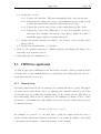
level, there is the whole tank. It consists of the hull, two treads and the rotatable
turret. The vertically movable gun is mounted in the turret. Figure 3-1 depicts a
possible scene graph representation for this setup.
Figure 3-1: Scene graph representation of a tank
Because of its hierarchical structure, using a scene graph also allows for some performance optimizations in the rendering process. If each node stores the bounding box of
itself including all descendants, whole objects or parts of them may be easily skipped
if it is determined that a bounding box lies completely outside the camera’s viewing
frustum. This technique can also be used for faster intersection or collision queries.
3.3 3D audio
3D audio allows placing sound sources and the listener (the audio analog to the camera in 3D graphics) within three-dimensional space. By using filters and by changing
the volume and frequency of the sounds, very realistic effects can be achieved, which
make this technology an important part of virtual reality applications [12]:

Attenuation: The perceived volume of a sound decreases with its distance to the
listener.

Doppler effect: If a sound source moves towards the listener (or vice versa), its
sound waves get compressed, which leads to a higher frequency. In opposite, if the
source moves away from the listener, the waves get stretched, leading to a lower
frequency.
Page 18

Methods and tools
Head-related transfer function (HRTF): If a sound comes from the left, it
reaches the left ear earlier than the right ear. Also, since the sound waves have to
pass the head, they get filtered, and the right ear perceives the sound differently.

Reverberation: This effect can simulate the influence of the geometric environment the sound is played in. For example, when a sound is played within a closed
room, the sound waves will be reflected off the walls.
3.4 Physics simulation
For the simulation of the bicycle and for collision detection, a physics engine should
be used. Otherwise, very complex differential equations would have to be solved “manually”.
A physics engine’s task is to simulate the dynamics of objects realistically, including
effects like gravity, friction and inter-object collisions [13]. Since such a physical simulation quickly becomes very expensive, trade-offs between realism and speed have to
be found. Physics engines that are used in computer games concentrate on achieving
real-time frame rates.
Most physics engines share some common concepts. The understanding of these concepts is vital for successfully integrating a physics engine into a simulation application.
3.4.1
Rigid bodies
Rigid bodies are non-deformable bodies and serve as the representatives of solid objects in the physics engine (for example, the moving parts of a bicycle). The motion
of rigid bodies is described by rigid body dynamics. In the real world, every object is
deformable to a certain extent, so the concept of rigid bodies already is an approximation.
Some physics engines can also simulate deformable bodies (soft bodies) by
representing them as a cloud of points connected by springs, but this comes with a
noticeable computation overhead and is not required for the purposes of FIVISim.
Therefore, the word “rigid” will be left out from now on, because rigid bodies are the
only ones that are going to be used.
Methods and tools
Page 19
Table 3-1 lists the translational and rotational quantities of bodies.
Table 3-1: Translational and rotational quantities of rigid bodies
Translational
Rotational
Attribute, symbol
Unit
Description
Attribute, symbol
Unit
Description
Mass m
kg
The relationship beMoment of inertia I
tween acting forces
kg m 2
and resulting accelerations.
The relationship between
acting torques and resulting angular acceleration
(“angular mass”), determined by the distribution
of mass.
Position x
m (vector)
Position of the body’s
center of gravity.
Orientation R
1 (rotation matrix)
The orientation of the
body’s local coordinate
system relative to the global coordinate system.
Linear velocity v
m
(vector)
s
Change of position of
the body’s center of
gravity per second.
Angular velocity ω
rad
(vector)
s
Axis and speed of rotation
(vector direction and
length).
Bodies are influenced by forces and torques. Applying a force to a body results in an
acceleration according to Newton’s second law, F= m ⋅ a . Likewise, a body can be rotated by applying a torque τ .
Gravity, which is approximated as being a homogenous field, is set globally and
m ⋅ g , where g is
creates a force acting upon each body according to the equation F=
g
the gravity vector. An approximate gravity vector on the earth’s surface is
(0
−9.81 0 ) sm2 , with the y-axis pointing up.
One important thing to notice is that a body doesn’t have a shape, because it isn’t
relevant to how it reacts to forces and torques. However, a body’s mass distribution
is relevant for rotations. It is reflected by the moment of inertia.
3.4.2
Shapes and materials
Shapes are handled separately from bodies. They are only significant for collision detection and response. Each shape is assigned to a body and moves along with it.
When the physics engine determines that two shapes collide, it applies forces and
torques to their bodies in response to the collision.
Page 20
Methods and tools
Depending on the physics engine, a different set of shape types may be available. The
most common shapes are planes (used for modeling an infinite ground), boxes,
spheres, capsules (cylinders with one half-sphere at each cap), convex shapes and arbitrary triangles meshes. The latter should generally be avoided if possible, since collision detection with arbitrary triangle meshes is more expensive and less accurate.
Consequently, it is advisable to decompose complex shapes into a set of simpler convex shapes.
Most physics engines allow assigning a material to a shape. Material parameters determine the friction and elasticity of collisions. Elasticity, or restitution, determines
the amount of kinetic energy that will be preserved during the collision. For example,
if a rubber ball hits asphalt, it will bounce (preserving most of its kinetic energy) and
eventually begin to roll because of friction. But if a stone is thrown at a frozen surface, the collision will be less elastic, and since there will be almost no friction, it will
begin to slide.
3.4.3
Joints
If an object is to be simulated that is composed of several movable bodies, such as a
bicycle consisting of a frame, a handle bar and two wheels, these bodies’ relative motions have to be constrained. The bicycle’s wheels can only rotate around one fixed
axis and can’t be translated at all. Accordingly, five out of six degrees of freedom
must be removed. The handle bar motion is restricted to rotations around the steering axis (and possibly up and down for suspension), but the steering angles have to
be limited.
Physics engines offer joints in order to achieve these kinds of constraints. Joints connect two bodies and restrict their relative translational and rotational motion. Depending on the joint type, different degrees of freedom are removed or limited. Many
physics engines also support motorized joints, which is a useful feature for modeling
vehicles.
3.4.4
Discrete time steps
Physics engines simulate their world using discrete time steps. Usually, some simulation function has to be called, taking a parameter
the time interval to be simulated.
∆t
that determines the length of
Methods and tools
Page 21
In order to simulate a time step, the physics engine has to perform a number of tasks:

Collision detection: The physics engine finds pairs of intersecting shapes. A
naïve O (n 2 ) algorithm would test each pair of shapes in the scene for intersection.
But since intersection tests tend to be costly (especially with complex shapes like
triangle meshes), spatial acceleration structures such as grids or octrees are utilized for quickly identifying pairs of potentially colliding shapes. For each collision,
contacts are generated that store the collision details (position, normal, amount of
penetration, relative velocity, friction and restitution). If objects move fast, continuous collision detection (CCD) techniques should be applied in order to prevent
them from flying through each other.

Collision response: For each contact, forces and torques are applied to the bodies for resolving the collision. The amounts depend on the collision parameters.

Enforce constraints: Bodies that are connected by a joint must not violate the
joint’s constraints. If a body does so anyway, the physics engine applies a force or
torque in order to bring it back into an allowed position or orientation.

Update bodies: Each body’s position, orientation, velocity and angular velocity
values are updated according to the forces and torques acting upon them.
3.4.5
Potential problems
Using a robust physics engine can facilitate the development of a simulation application like FIVISim extremely. However, there are a few things that one should be
aware of.

Determinism: Physics engines are not necessarily deterministic4. For example,
there may be a different simulation result when simulating ten time steps of 0.1
seconds each compared to when simulating a single time step of one second. This
is mainly due to collision detection and numerical accuracy. But even with equally-sized time steps, the simulation may behave differently from time to time, because the physics engine could internally use a random number generator in certain ambiguous situations.
Of course, every computer program is deterministic, since computers are deterministic. In this case,
determinism means that the same user input always leads to the same output.
4
Page 22

Methods and tools
Conflicts with scene graphs: Scene graphs use hierarchy to represent geometric object dependencies. In the example discussed earlier, the turret is a child of
the tank. When the tank moves, the turret moves along with it. Actually, this is a
very simplistic approach to physics simulation. On the other hand, in a real physics engine, such dependencies are modeled with joints, which is physically more
accurate. These concepts are incompatible. On the level of physically simulated
objects, the scene graph therefore has to be flat. However, on the visualization
level, a scene graph sub-tree could be attached to one single physical object. In
the tank example, there could be a rotating radar dish on top of the turret. If it
doesn’t need correct physical simulation, then it can be represented only by a
scene graph node, which is a child of the turret node.

Authority: If a physics engine is used, it should be given the final say about the
positional and rotational quantities of the bodies it simulates. That means that,
although physics engines allow this, the position, velocity, orientation and angular
velocity of bodies should not be set from outside, except for initialization or to
perform a “reset”. Calculating these quantities is the physics engine’s responsibility. If the program interferes with that, it could as well use no physics engine at
all. Manipulating bodies should only be done by applying forces, torques and impulses or by the means of joints.
3.5 Bicycle dynamics
Bicycle dynamics describe how a bicycle reacts to forces applied to it. Today, physicists still disagree about how bicycle stability is governed by certain effects, so the topic is more complex than it may seem to be. The following introduction is based on
the works of Fajans [7] and Franke et al. [6]. It will concentrate on self-stability, the
geometric properties of a bicycle, turning, steering and leaning.
3.5.1
Self-stability and geometric properties
Bicycles exhibit a self-stabilizing behavior for certain speeds. Self-stability means that
the bicycle will keep upright by itself, without any steering torques or shifting of
weight applied by the rider. In fact, the rider can even be completely removed.
Methods and tools
Page 23
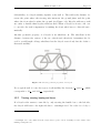
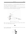
Self-stability of a bicycle mainly depends on its trail T . The trail is the distance between the point where the steering axis intersects the ground plane and the point
where the front wheel touches the ground (see Figure 3-2). Bicycles with more trail
are easier to handle than bicycles with less trail. When a bicycle is about to tilt over
to one side, the trail compensates by making the front wheel steer to this side automatically.
Another geometric property of a bicycle is its wheelbase W . The wheelbase is the
distance between the centers of the two wheels and effectively determines the bicycle’s overall length. A huge wheelbase lets the bicycle react slowly but also leads to
increased stability.
Figure 3-2: Selected geometric properties of a bicycle
For a typical trail of 6 cm, the region of self-stability lies between 5 ms and 6 ms , which
corresponds to 18 kmh and 21.6 kmh , respectively.
3.5.2
Turning, steering, leaning and forces
If a bicycle rider wants to turn left by only steering the handle bar to the left side,
the bicycle will lean to the right side due to centrifugal force 5. In order for a body to
Centrifugal force only exists from the bicycle rider’s point of view. Actually, it is the result of the
missing centripetal force.
5
Page 24
Methods and tools
follow a circular path (a turn can be treated as one), a certain amount of centripetal
force has to be applied towards the center point of the turn. Therefore, in order to
make a left turn, the rider has to momentarily steer to the right side. Since the bicycle is now turning right, centrifugal force leans it to the left side. This process is
called countersteering. With the correct lean angle λ , the friction force exerted by
the ground and the tires provides the centripetal force needed. The front wheel reacts
to the leaning by steering into the desired direction. Now, the bicycle is turning.
The torques that the rider has to apply to the handle bars in order to steer, are very
small. This is why a bicycle can also be ridden no-handed, by just using the hips or
weight shifting in order to initiate a turn.
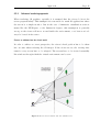
Figure 3-3 shows the forces that are involved in turning. The bicycle is stable and is
considered as a single rigid body, for simplification. Fg is the gravitational force directed downwards, which depends on the bicycle’s mass m and the gravity vector g :
F=
m⋅g
g
The ground exerts a reaction force Fn to the bicycle. It is directed upwards and has
the same magnitude as Fg . Additionally, there is a friction force Ff , directed away
from the center of the turn. If the bicycle is completely upright, meaning that λ = 0 ,
then Ff = 0 .
Figure 3-3: Forces acting upon the bicycle while turning
In order for the bicycle to follow the circular path of the turn, the centripetal force
Fc
has to be applied. It is directed towards the center of the turn. Its magnitude de-
pends on the curve radius r , the bicycle’s mass and its velocity v .
Methods and tools
Fc =
Page 25
m ⋅ v2
r
The friction force has to provide the necessary centripetal force, so Ff = Fc . Since the
forces Fn and Ff do not attack at the center of gravity, they both exert a torque on
the bicycle. The magnitudes of these torques τn and τf are (force times lever arm):
τn = Fn ⋅ sin λ = m ⋅ g ⋅ sin λ
m ⋅ v2
⋅ cos λ
r
τf =Ff ⋅ cos λ =
The torques have to cancel out each other. Otherwise, the bicycle would tilt over to
one side. Thus, by equating the torques, the required lean angle λ can be determined:
τn = τf
m ⋅ v2
⋅ cos λ
r
⇔ m ⋅ g ⋅ sin=
λ
⇔ g ⋅ sin λ =
v2
r
⋅ cos λ
sin λ v2
=
cos λ
r
v2
⇔ g ⋅ tan λ =
⇔ g ⋅
r
⇔λ=
arctan
v2
g ⋅r
This term for λ can later be used in the simulation to make the virtual bicycle lean
correctly, since the real bicycle is fixed and cannot lean.
Approach
4
Page 27
Approach
In this chapter the approach for solving the problems discussed in chapter two is developed, using the methods and tools presented in chapter three. It proposes a
layered simulation model, in which each layer adds new functionality to the simulation by using the layers below. The bicycle physics will be simulated using rigid body
dynamics. An algorithm for perspective-correct visualization is presented, as well as
an approach for exposing bicycle riders to scalable physical and psychological stress
factors.
4.1 Layered simulation model
As discussed in chapter two, for objects in the virtual world, such as bicycles and
cars, a number of requirements have to be met:

They should group various physical sub-objects (bicycle: frame, wheels, handle
bar) and coordinate their interaction in order to function as a whole. So, for example, the bicycle becomes able to accelerate, brake and steer.

Different behaviors should be decoupled from the objects themselves.

The semantics of events occurring in the virtual world and the overall simulation
control should be left completely undefined by the simulator, since they depend
entirely on the concrete scenario.
In order to fulfill these requirements, a layered approach has been chosen, with each
layer extending the previous one and reflecting certain aspects of an object and the
simulation. This approach is similar to the OSI Reference Model 6 used in the design
of network protocols. The simulation is divided into the physical layer (physical
properties of objects and visualization primitives), the logical layer (grouping physical
objects and providing basic actions), the control layer (generic object control) and the
semantic layer (simulation control and reaction to events). Each layer will be described in the following.
6
http://www.itu.int/rec/T-REC-X.200-199407-I/en
Page 28
4.1.1
Approach
Physical layer
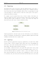
The physical layer is the bottom layer. Only the physical movable object parts, or
sub-objects, are of interest. A physics engine is used in order to simulate the interactions between these sub-objects, including collisions. They are approximated by rigid
bodies and shapes for collision detection. Joints can connect pairs of sub-objects to
restrict their relative movements.
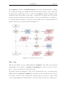
For example, from the physical layer view, a bicycle consists of the frame, two
wheels, the handle bar and an optional rider. Each of these rigid bodies has a shape.
Joints keep them together. On this layer, a “bicycle” object doesn’t exist. Figure 4-1
shows the bicycle’s sub-objects. Joints are indicated by lines.
Figure 4-1: Physical layer view of bicycle sub-objects
Visual representations of the sub-objects, in form of 3D meshes, are also included in
this layer. In summary, the physical layer contains the primitive physical and visual
building blocks that form a more complex object.
4.1.2
Logical layer
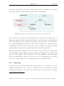
On the logical layer, physical sub-objects are combined into one logical object, which
is given a name, or ID (for example “bike1”). This logical object can manipulate its
sub-objects or the joints connecting them. In this way, it can provide some basic
functionality. This functionality describes an interface.
As an example, consider the bicycle object again. The logical bicycle object groups
the afore-mentioned physical sub-objects and can manipulate them in order to provide basic functions, such as “accelerate”, “brake” or “steer”. For instance, the joint
that connects the handle bar to the frame, can be manipulated in order to steer, and
for acceleration, the joint between the back wheel and the frame can be motorized
Approach
Page 29
(see Figure 4-2). The logical bicycle object will also have to attain the correct lean
angle when turning, but this will be discussed later in this chapter.
Figure 4-2: Logical bicycle providing steering and acceleration functionality
Since a logical object knows the relationships and the meaning of its sub-objects, visualization primitives will be kept synchronized to their physical counterpart here,
since both the rigid bodies and the scene graph nodes store their own transformation 7. The synchronization is needed in order for the visualization to match the physical simulation. This is done by the logical object, for example by using a map data
structure that stores pairs of associated rigid bodies and scene graph nodes.
Playing sounds is also handled by the logical layer. Logical objects can emit sounds
and dynamically change their properties (volume and frequency). For example, the
sound of a car’s engine could be adapted to its speed. Similarly to the scene graph
nodes, all sounds that are played by an object need to be synchronized to the physical object’s position and velocity, which is important for the Doppler effect.
4.1.3
Control layer
Logical objects provide basic functionality, but they have to be told what to do from
a higher level. Therefore, the concept of “controllers” has been developed. Controllers
encapsulate the behavior of a logical object. They exist on the control layer. An arbi-
7
This is redundant, but can’t be avoided when using separate libraries for 3D graphics and physics.
Page 30
Approach
trary number of controllers can be attached to a logical object and control it using
the functionality it provides.
Artificial intelligence can be implemented using the concept of controllers. For example, in order to make a logical car object drive through the virtual environment along
a certain route, a special controller type could be implemented and assigned to the
car object. In the case of the bicycle object, different controllers could either allow
controlling the bicycle via the FIVIS hardware or via the keyboard (see Figure 4-3).
Figure 4-3: Logical bicycle object being affected by controllers
By separating the behavior from the object itself, expandability is increased. A single
logical object type can be paired with a number of different controller types, and each
combination produces a differently behaving object.
One interesting possibility that emerges from the controller concept is recording and
playing back user input. This might prove very useful in the road safety education
scenario: A passive recording controller continuously samples the bicycle’s input parameters (steering and acceleration) and writes them to a file. Later, when the recorded ride should be played back for review and discussion of mistakes, an active
playback controller is used. It reads the data file previously stored and applies them
to the virtual bicycle. Provided that the simulation is deterministic (see 3.4.5), the
playback will exactly match the original ride.
Approach
4.1.4
Page 31
Semantic layer
Using the three layers described so far, logical objects such as bicycles and cars can
navigate through the virtual world and can be controlled in different ways. What is
still missing is a global instance that gives semantics to events happening in the virtual world and reacts to them accordingly. This takes place in the semantic layer.
To justify the existence of the semantic layer, consider the road safety education scenario again. If the rider jumps the lights, a reaction to this event might be required,
for example playing a police siren sound or using the motion platform to catapult the
rider off the bicycle. This kind of reaction is totally specific to the scenario and
should therefore neither be the traffic light object’s responsibility, nor the bicycle object’s.
The semantic layer can be regarded as the global framework that uses the services
provided by the simulation in order to put it in a context such as road safety education or the stress research scenario. In general, it will not have to do any complex
computations, so its implementation could easily be written in the scripting language.
4.2 World concept
Some instance has to manage all the virtual objects in a scene. In the simplest case,
this means iterating over them and telling them to update themselves. When an object is no longer needed, it has to be removed and deleted. Also, due to the nature of
most physics engines, the physics simulation has to be triggered globally, not on a
per-object level.
This is where the concept of worlds comes into play. A world manages its virtual objects, tells them to update themselves from time to time and drives the physics simulation. It also allows objects to access other objects. For example, a car that drives
through the city needs information about where the other cars are, in order to avoid
collisions. It should therefore be possible to get a list of objects from the world or retrieve an object by providing its ID.
The world also provides events that the objects or the semantic layer application can
subscribe to. For example, some tasks might have to be performed once every simulation time step. Therefore, the world continuously triggers an “update” event.
Page 32
Approach
4.3 Expandability
Since FIVISim will be used in many different contexts, it has to be very expandable.
One concept of expandability has already been presented: the use of controllers as
abstractions of behavior. The design decisions made in order to support this and other concepts are discussed in the following.
4.3.1
Factories
The factory design pattern allows creating instances of classes that are unknown to
the program at compile time [14]. This pattern can be found in the design of many
programs that allow external plug-ins to enrich the palette of creatable objects, like
additional geometry types in a 3D modeling product.
Creating objects and controllers will be accomplished using the factory pattern. For
example, there may be a user-defined object type called AirplaneObject. When an
object of this type is encountered while loading a world, the list of registered object
factories is searched for one that can create an object of the type AirplaneObject.
If such a factory is found, the task of creating the object is delegated to it.
4.3.2
Events
Often, one object or the semantic layer might be interested in events happening in
the simulation. For example, a traffic light object could provide an event that is fired
whenever some vehicle passes it while the light is red. A police car nearby would then
subscribe to this event in order to get informed and react. This can be solved using
the observer design pattern [14]. Another event that will be implemented is the collision event that is triggered when an object collides with another.
4.3.3
Data representation
A way has to be found to store world and object descriptions in a file. This is important, since separating content from simulation logic also means better expandability.
Approach
Page 33
XML 8 presents itself as a candidate for the task, as it is expressive, commonly known,
simple to learn and easy to parse. There are many already finished parsers available.
Without the use of XML or a similar language, a custom parser would have to be
implemented. Additionally, XML is human-readable and can be easily written by
plug-ins for third-party software. Readability is particularly helpful during the application development process, whereas a lot of classes and attributes are undergoing
frequent changes.
Listing 4-1 shows how such an XML document, describing a world with a bicycle object, might look like. The world, the bicycle and its controllers each have an XML
representation, and therefore must be able to initialize themselves from it.
Listing 4-1: Example world XML description
<?xml version="1.0" encoding="utf-8" ?>
<World>
<AmbientLight color="(0.7, 0.7, 0.7)" />
<Sunlight color="(1, 1, 1)"
direction="(0.8, -1, 0.5)" />
<Objects>
<BikeObject id="bike"
position="(0, 1, 10)"
direction="(0, 0, 1)">
<Controllers>
<HardwareBikeController />
<BikeRecordingController filename="bike_log.txt"
logFrequency="60" />
</Controllers>
</BikeObject>
</Objects>
</World>
At the top level, there is a World element. It contains information about the lighting
(AmbientLight and Sunlight) as well as a list of objects. Objects have an ID (a
unique identifier that can later be used to retrieve the object), a position and a direction. Inside the BikeObject element, a list of controllers follows. In this example,
there are two controllers attached to the bicycle: a HardwareBikeController and a
BikeRecordingController. These controllers could have additional attributes or
inner elements, if necessary. However, this XML document is just an example, intended to clarify the concept.
8
http://www.w3.org/TR/2006/REC-xml-20060816/
Page 34
Approach
4.4 Bicycle model
The virtual bicycle is simulated using a physics engine, instead of solving the differential equations presented in many works related to bicycle dynamics. That means
that it is entirely modeled by rigid bodies and joints. The bicycle is therefore consistent with the rest of the virtual world. It can be steered and accelerated by manipulating the joints and bodies.
In theory, the bicycle should behave as predicted by the models presented by Fajans
[7] and Franke et al. [6], provided that the physics engine is accurate enough.
4.4.1
Rigid body setup
The bicycle model consists of four bodies: the frame, the handle bar and the two
wheels. The handle bar is attached to the frame, and the front wheel is attached to
the handle bar. The back wheel is attached to the frame directly.
Frame
The frame is the bicycle’s “main” body. It is the heaviest of all bodies, since it also
accounts for the rider. Experiments with a separate body representing the rider led to
a rather unstable behavior of the bicycle, so the rider and the frame are merged into
a single body. A convex mesh shape is used for collision detection and mass distribution.
Handle bar
The handle bar is connected to the frame by a revolute joint. This kind of joint restricts the connected bodies’ motions to rotations around a fixed axis. In the case of
the bicycle, this is the steering axis. It is not aligned vertically in order to create the
trail. The joint is configured in a way that allows specifying a target angle. A simulated spring then pushes the handle bar into the according position. The handle bar is
represented by a convex mesh, too.
Wheels
A motorized revolute joint connects the front wheel to the handle bar. For braking,
the motor is activated with a zero target velocity. Another motorized revolute joint
Approach
Page 35
connects the back wheel to the frame. It both accelerates and decelerates the bicycle,
depending on the difference between the current speed and the target speed.
Much attention has to be paid to the geometric properties of the wheels. Several
geometric shapes have been tested in the prototype: spheres, ray casting wheels and
convex wheel-like ellipsoids.
The ray casting wheels work by casting a ray from the wheel’s center downwards and
evaluating its intersection with the world geometry. Friction forces are then determined accordingly. However, the ray casting wheels are meant for car racing games
and generally lead to an arcade-like behavior.
Using a convex mesh, the flat shape of a bicycle wheel can be modeled closely. But
convex meshes are not smooth, since they are represented by a finite (and often very
limited) number of plane equations. In experiments during the development of the
prototype, the bicycle exhibited rather bumpy ride characteristics, so this solution
was discarded.
Spherical shapes turned out to be the best solution. Even though their geometric
form doesn’t correspond to that of a real wheel, they make for a smooth rolling behavior. Therefore, the physical representation of a wheel will be spherical.
Figure 4-4: Physical bicycle model
Page 36
4.4.2
Approach
Steering and lean angle
As discussed in chapter three, a bicycle needs to lean in order to turn. This is
achieved by countersteering. In order to make the bicycle turn left, one has to steer
right for a little moment. The front wheel will steer to the left side automatically after short time. Bicycle riders do the countersteering intuitively.
In an early phase of the first simulator prototype, the steering angle measured by the
potentiometer sensor was applied to the handle bar without manipulating the virtual
bicycle in any other way. It was possible to keep the bicycle upright and turn it, but
not in an intuitive way. It seemed that the countersteering is very subtle, or that
people simply don’t do it at all when they are on the fixed FIVIS bicycle. Furthermore, a real bicycle performs some moves automatically, if it is moving. Additional
actuators would be required to simulate that. Therefore, a compromise must be
found.
The approach used in FIVISim is a simplification. The rider uses the handle bar to
indicate the desired direction of travel. The simulator software will then manipulate
the virtual bicycle accordingly. This is, at least in principle, comparable to the digital
flight control systems found in modern airplanes. The pilot uses the joystick for telling the computer what he wants the airplane to do, and the computer then calculates
a solution and adjusts the elevators and the rudder accordingly. It can even prohibit
maneuvers that would be too dangerous.
Calculating the lean angle
The first problem that has to be solved is to determine the correct lean angle λ for a
given steering angle σ . This lean angle then has to be applied to the virtual bicycle
in order to make it turn instead of tilting over.
In chapter three, a term has been derived that expresses the lean angle depending on
the curve radius r :
λ = arctan
v2
g ⋅r
The squared velocity v2 and the gravity vector g can be easily obtained by querying
the physics engine.
Approach
Page 37
However, the curve radius has to be determined manually. Actually, there is one
curve radius for each wheel, as they don’t follow the same path. In the following, the
curve radius of the back wheel will be determined.
As shown in Figure 4-5, the bicycle’s longitudinal axis and the radii of the front and
the back wheel form a right-angled triangle. Since every triangle’s inner angles sum
up to 180°, the angle between the radii equals the steering angle σ .
Figure 4-5: Determining the curve radius
With one known side length and two known angles, the triangle is fully determined,
and r can be calculated using trigonometry:
r =
W
tan σ
Now, the required lean angle λ can be expressed in terms of the velocity, steering
angle, gravity and wheelbase:
λ = arctan
⇔λ=
arctan
v2
g ⋅r
v2
g ⋅
W
tan σ
2
v ⋅ tan σ
⇔λ=
arctan
g ⋅W
Page 38
Approach
Leaning the bicycle
Once the lean angle has been determined, the bicycle has to be manipulated accordingly. The bicycle’s current lean angle λ0 is calculated by taking the arccosine of the
dot product of the bicycle’s x-axis in world coordinates and the normalized gravity
vector, and then subtracting
π
2
. Then, a torque is applied to the bicycle that is pro-
portional to the square of the difference between the target lean angle and the current lean angle, that is ( λ − λ0 )2 . This way, larger deviations are compensated more
quickly. Additionally, in order to prevent oscillation, the bicycle frame’s angular velocity is damped by means of the physics engine.
4.4.3
Head wind sound
Computer games often use a simple, yet effective method for intensifying the user’s
perception of speed, by playing a head wind sound and adjusting its volume and frequency dynamically according to the speed. This approach will also be realized in
FIVISim. Therefore, a looping head wind sound is attached to the bicycle and updated constantly.
4.5 Visualization
As discussed in chapter two, visualization plays a crucial role when creating an immersive application like FIVISim aims to be. In the following, a concept for controlling and aligning the virtual cameras will be developed.
4.5.1
Camera object
In a typical scene, there may be a number of objects that can provide a view for the
visualization. In most cases, the camera should be placed on the user’s virtual bicycle,
but it should not be fixed. For example, it might be interesting to view the scene
from an AI-controlled car, or fly around freely using some kind of 6DoF (six degrees
of freedom) input device.
For this to be possible, one object at a time will be marked as the world’s camera
object. The visualization uses this object to determine the point of view and the viewing direction when rendering a frame. Now, every object can manage an arbitrary
number of proxy objects that don’t serve any purpose except being used as a camera.
Approach
Page 39
For example, a car could provide a number of camera objects: one being located at
the driver’s seat, one shooting from behind and one from above. It would be easy to
make the camera perspective change upon the press of a key.
4.5.2
Simple rendering approaches
Rendering images with the correct perspective to the projection screens provided by
the FIVIS system turns out to be a challenge, because they are not angled in 90° (as
in the Immersion Square) and the user is not always located in their center. Figure
4-6 shows a top view of the FIVISquare.
Figure 4-6: Top view of the FIVISquare
Approach 1: Rendering only once
The simplest approach is to simply ignore that the screens are angled and treat them
like one huge planar screen, using a standard wide-angle projection. This is what
happens when ordinary 3D applications are run in the FIVISquare, since they are
unaware of the fact that the image on the huge screen provided by the TripleHead2Go device really is split up and projected onto three individual angled screens.
Obviously, this simple approach (see Figure 4-7) leads to distortions at the side
screens when used in the FIVISquare.
Page 40
Approach
Figure 4-7: Single wide-angle rendering, limited to 180°
Additionally, due to the assumption that there is only a single planar screen, the horizontal field of view is always smaller than 180°. However, depending on the viewer’s
head position in the FIVISquare, the horizontal field of view can exceed 180°.
Approach 2: Rendering three times
If different cameras are used for rendering the images for the left, center and right
screen, the result is more convincing. The single wide-angle camera with a field of
view of, for example, 150° horizontally and 35° vertically, is replaced by three cameras covering 50° horizontally and 35° vertically. The three sub-images are rendered
at the appropriate position in the frame buffer so that they are projected onto the
correct screen. Figure 4-8 shows the result. Notice that there are bends at the subimages’ edges. They are only visible because the paper the image is printed on is flat.
When viewed from inside the FIVISquare, the bends disappear.
Figure 4-8: Three separate renderings combined, not limited to 180°
However, even this approach is not always correct. It produces wrong results if the
user’s head is not located at the center of the screens (the point where the three lines
from each screen’s center along its viewing direction meet, see Figure 4-6).
Approach
4.5.3
Page 41
Advanced rendering approach
When rendering 3D graphics, typically it is assumed that the viewer looks at the
screen perpendicularly. This assumption is reasonable for usual 3D applications where
the screen is a simple monitor. But in the case of immersive visualization environments like the FIVISquare or the Immersion Square, this assumption is generally
wrong, as the viewer will move around inside the environment, or at least won’t always be located in its center.
Screens as windows into the virtual world
In order to achieve a correct perspective, the viewer’s head position has to be taken
into account when rendering the 3D images. If the viewer moves, the viewing frustums for every screen have to be adapted. The screens have to be treated essentially
like windows through which the virtual environment can be seen.
Figure 4-9: Screen as a window into the virtual world
Page 42
Approach
Figure 4-9 shows the viewer in two different positions, looking at the same screen.
From position 1, the view direction is perpendicular to the screen surface. The viewing frustum is symmetric, meaning that the angles between the lines to the screen
edges and the screen center are equal (27° both). The viewing frustum from position 2
is asymmetric, as the angles differ (14° and 23°, respectively). Depending on the position, different objects can be seen. For example, the above tree can only be seen from
position 2, and the below tree can only be seen from position 1.
Viewing frustum description
Geometrically, the viewing frustum is a pyramid limited by two planes parallel to its
base. The viewer is located at the pyramid’s apex. The form of the frustum defines
how the 3D geometry is projected onto the 2D image plane (the perspective projection). Viewing frustums can be described using 9 parameters (see Figure 4-10).

Viewer position E : The position of the viewer, or the camera, in world space
coordinates.

View direction v and up vector u : These vectors define the viewer’s orientation. v is essentially the viewer’s z-axis, and u is the viewer’s y-axis, in world
coordinates. Note that the x-axis doesn’t need to be specified explicitly, as it can
be calculated from the other vectors by taking the cross product.

Distances of near and far clipping planes dnear and dfar : The viewing frustum is cut off at these distances. Any geometry nearer than dnear or farther than
dfar will not be displayed on the screen.

Frustum extents fleft , fright , ftop and fbottom : The frustum extents affect the frustum’s horizontal and vertical opening angles and its center. The extents define the
x and y coordinates where the viewing frustum intersects the near clipping plane,
in the viewer’s local coordinate system. For example, if fleft = −1 , fright = 1 and
dnear = 2 , the frustum is symmetric on the horizontal axis and has an opening angle
of 90°.
If all these frustum parameters are known, a camera and perspective projection matrix can be constructed and used for rendering 3D geometry.
Approach
Page 43
Figure 4-10: Explanation of the viewing frustum parameters
Representing arbitrary screens
In order to make the FIVISim visualization as flexible as possible, rendering to arbitrary aligned screens will be supported. The visualization will not be limited to the
screen setup found in the FIVISquare. It will render perspective-correct images for
any other visualization environment, independent of the number of screens, their size,
position and orientation, as long as the screens are rectangular and perpendicular to
their projector. Screens can then be described by three parameters (see Figure 4-11):

Center position C : The screen’s center point.

Half-size vectors h x and h y : These vectors point from the screen’s center to its
right and top edge, respectively. Their length determines the screen size. For the
0 ).
screen to be rectangular, these vectors have to be orthogonal ( h x ⋅ h y =
Page 44
Approach
Figure 4-11: Explanation of screen representation parameters
Additionally, the viewport rectangle of the screen is stored. It defines the region in
the frame buffer that will receive the image rendered for the screen. By choosing the
viewport rectangle according to the image split positions used by the Matrox TripleHead2Go unit, each projection screen receives the correct image (Figure 4-12).
Figure 4-12: Displaying the correct image on each projection screen
Determining the viewing frustum
Now, the viewing frustum parameters have to be determined in terms of E , C , h x
and h y . Since the viewing frustum passes through the screen, the view direction v
equals the negated normal vector of the screen, and the up vector u is h y normalized.
Approach
Page 45
v=
− h x × h y ⇔ v =h y × h x
u = hy
The near clipping plane distance dnear is the distance between E and the screen plane.

It can be calculated by projecting the vector EC onto v :

dnear
= EC ⋅ v
The far clipping plane distance dfar can be chosen arbitrarily, although it should not
be set too high in order to limit the visible part of the scene. It defines the range of
sight, which can for example be 1000 meters. The remaining parameters, the viewing
frustum extents, can be figured out by projecting the viewer position E onto the
screen plane, yielding the point E′ , and then calculating the distance from E′ to the
screen’s left, right, top and bottom edge, respectively.
E′ = E + d ⋅ v
fleft = ( C − h x − E′ ) ⋅ h x
fright = ( C + h x − E′ ) ⋅ h x
fbottom = ( C − h y − E′ ) ⋅ h y
ftop = ( C + h y − E′ ) ⋅ h y
Using these equations, the viewing frustum parameters can be calculated for each
screen that will be rendered to.
4.5.4
Depth perception
In order to perceive depth in a scene, the human visual system uses a great number
of visual cues [15]. These can be divided into monocular (requiring only one eye) and
binocular cues (using information from both eyes). Depth perception increases the
user’s presence, since it makes the virtual world look more real. Since stereoscopy is
not planned to be used in FIVIS, only monocular cues can be used:

Motion parallax: Moving through a scene and observing the apparent relative
motion of static objects provides indications for their spatial relationships. This effect is achieved automatically using 3D graphics, due to perspective projection.
Page 46

Approach
Relative size: When an object appears to become larger, it is probably coming
closer. Also, when the real size of an object is known, its distance can be judged.
This is achieved by perspective projection, too.

Aerial perspective: With increasing distance, objects lose contrast and color
saturation due to light scattering in the atmosphere. This can be simulated with
depth fog, which is a standard feature of graphics APIs.

Occlusion: Objects that are closer to the observer occlude objects farther away.
In 3D graphics, this effect is usually obtained by using a z-buffer.

Peripheral vision: Peripheral vision provides unfocussed, visually distorted images, but is important for the perceived presence. The FIVISquare screens cover a
huge part of the peripheral visual field so that the bicycle rider can perceive a
consistent visual impression.

Lighting and shadows: While in computer vision a frequent task is to eliminate
shadows from an image, in computer graphics considerable effort is undertaken to
generate them in order to provide realistic lighting. This effort is justified, since
shadows provide the viewer some important hints about the position, size and
spatial relationship of objects [16]. Lighting and shadowing are features found in
almost every 3D engine.
4.6 Simulation loop
The simulation loop consists of the tasks that have to be done on a per-frame basis.
It combines all the concepts that have been presented so far. This is where the actual
simulation and visualization take place.
In particular, the following tasks are performed in the simulation loop:
1. Send rendering calls to the graphics API. They are executed in the background by
the graphics hardware. Meanwhile, the actual simulation can be executed on the
CPU.
2. Update the world:
2.1. Perform a physics simulation time step. All physical interactions between objects are computed.
2.2. Trigger the “update” event.
2.3. Inform objects that collided during the physics simulation step.
Approach
Page 47
2.4. Update the objects:
2.4.1. Update all controllers. They may manipulate their object in any way.
2.4.2. Transform the visual sub-objects’ representations (scene graph nodes)
so that they match their physical representations (bodies).
2.4.3. Update the position and velocity of all sounds played by the object.
2.4.4. Update the object itself. What has to be done here depends on the actual type. For example, the bicycle object has to adjust its joints to
match the input values for steering and speed.
2.5. Update the virtual cameras according to the camera object and the user’s
head position.
2.6. Update the virtual listener, for 3D audio.
3. Wait for the graphics hardware to finish rendering and display the image. If a
screenshot was requested, save it.
4. Optionally quit the simulation loop.
4.7 FIVIStress application
A solution approach for FIVIStress, the stress factor scenario, will be presented in the
following part. A first implementation for generating and scaling physical and emotional stress has also been done.
4.7.1
Physical stress
Obviously, physical stress can be generated by requiring the user to pedal. The physical stress can be scaled in two ways: by adjusting the resistance exerted by the Tacx
Cycletrainer and by scaling the pedaling effect on the virtual bicycle. The latter is
more interesting, since it can be changed by the simulation software. The so called
“pedal factor” determines the relationship between the bicycle’s virtual and real (sensor-measured) speed.
virtual speed ⋅ pedal factor =
real speed
For example, if pedal factor = 2 , the user has to pedal two times as fast in order to
reach a certain virtual speed than he would have to in reality. It might be interesting
to investigate if the impact of this is motivating or discouraging.
Page 48
4.7.2
Approach
Emotional stress
In the following, a number of emotional stress factors are described that will be integrated into the simulation. In general, they are derived from stress factors known by
daily experience. If the user’s presence is strong enough, the virtual world situation
should evoke physiological reactions comparable to similar stress in the real world.
Each of the stress factors can be scaled independently.
City environment
Within the context of the FIVIS project, parts of the city of Siegburg have been
modeled with Google SketchUp, based on satellite images and photographs for the
building textures. The city environment has been converted to a suitable data format,
using a number of custom-written plug-ins. It will serve as the stage for the stress
factor scenario, since it looks natural to the user and allows for integrating a variety
of stress factors.
Pressure of time
As daily experience teaches, emotional stress increases when a task has to be accomplished within a limited time frame, even if the task itself is simple.
Within the city, a number of checkpoints are placed (see Figure 4-13). The user must
reach each checkpoint within a specific time. This should provide motivation for pedaling harder. Running out of time, the user might have to take risks in order to
reach the next checkpoint. A countdown sound effect signals that time is running
short. When the countdown reaches zero, a loud low-pitched tone is played. This
way, the checkpoints actually combine physical and emotional stress.
The time pressure stress factor can be scaled by dividing the time limit for each
checkpoint by a “time divisor” parameter. This could also be done increasingly (for
example: each minute, reduce the time limits by 5%). The checkpoints are arranged
in a circle so that there is no end, which allows for potentially very long test runs
within the limited virtual world.
Approach
Page 49
Figure 4-13: Example scene with five checkpoints
Evading cars
Cars are randomly spawned on a street that the user has to ride on. They drive in
the opposite direction and are quite fast. The user has to evade them. If a collision is
likely, the cars honk their horn, but don’t try to avoid the bicycle (see Figure 4-14).
Figure 4-14: Cars approaching the user’s bicycle have to be evaded
Although obviously not being realistic, this should expose the user to a certain
amount of stress. If a car hits the bicycle, valuable time for reaching the next checkpoint is lost. More complex traffic scenarios with intelligently behaving cars would
certainly make the experience more realistic, but will not be implemented until the
FIVIS traffic simulator is available.
Page 50
Approach
The spawning frequency ( car frequency ) and the speed of the cars ( car speed ) are variable. It may be interesting to see if increasing the car spawning frequency or speed also
increases the user’s stress.
Reacting to suddenly appearing obstacles
More stress can be generated if the user has to constantly pay attention to something
that might happen at any time. Therefore, falling boxes are randomly placed in the
user’s path. They emit a certain sound and cast a shadow onto the ground, so that
their position can be estimated. Their creation frequency ( box frequency ) is adjustable.
Sound volume
The overall sound volume can be changed in software (parameter volume ). Louder
sounds (car engines, horns) will probably lead to more stress. Table 4-1 summarizes
the different stress parameters.
Table 4-1: Overview of FIVIStress parameters
Parameter
Type of stress
Meaning
pedal factor
Physical
How much faster the user has to pedal, compared to normal.
time divisor
Combined
The time available to the user in order to reach each checkpoint
is divided by this value.
car frequency
Emotional
A new car is spawned every car frequency −1 seconds in average.
car speed
Emotional
The cars’ average speed.
box frequency
Emotional
A new obstacle box is spawned in front of the user’s bicycle
every box frequency −1 seconds in average.
volume
Emotional
Changes the overall sound volume.
4.7.3
Controlling the simulation
It should be possible to adjust all stress parameters at runtime, using some kind of
user interface. Since the entire screen of the simulation PC is occupied by the visualization, the user interface has to run on another computer. This can be achieved elegantly using network communication: A small client program runs, for example, on a
laptop that is connected to the same network as the simulation PC. Commands for
Approach
Page 51
changing simulation parameters are then generated from a user interface and sent to
the simulation PC, where they are processed.
4.7.4
Data logging
The sensor data measured by the CUELA system needs to be related to events happening in the bicycle simulation in order to allow a reasonable evaluation. Therefore,
important simulation data has to be identified and logged in a way that it is easily
retrievable.
Again, XML is an adequate candidate for the log data format. XML is commonly
used for representing data in such a way that it can be easily read by other applications. During the simulation, the following parameters will be logged:

Status samples: These samples contain status information about the bicycle
(current speed, input speed and steering angle), the next checkpoint that has to
be reached (its ID, distance and the time that is left), the closest car (ID, distance, speed and if it is honking or not) and the closest obstacle box (ID and distance). Status samples are logged at a frequency of status sample frequency .

Checkpoint events: These events are logged whenever the user reaches a checkpoint. They contain the exact time, the ID of the checkpoint and the time that
was left to reach it.

Collision events: Whenever the user collides with a car or an obstacle box, a
collision event is logged. The time of the collision and the object ID are stored.

Screenshots: A scaled-down version of the user’s complete view is saved to image
files at a frequency of screenshot frequency . The exact time and the screenshot filename are written into the log file. The screenshots should be useful for reconstructing the user’s route and help analyzing certain situations that can’t be easily
expressed in terms of numbers.

Parameter changes: When the stress parameters ( pedal factor , time divider , …)
are changed at runtime, the new values are logged.
The collection of these types of information, combined with the data recorded by the
CUELA system, should allow for an extensive analysis of the combined physical and
psychological strains.
Realization
5
Page 53
Realization
This chapter covers the realization of FIVISim and FIVIStress. First, it will evaluate
and describe the tools that will be used, including the programming and scripting
language and the graphics, sound and physics engines. After that, some implementation details will be depicted. Since there are is a huge number of classes involved in
FIVISim, not all of them will be discussed. Instead, only the most important parts of
the implementation will be focused on.
5.1 Languages and libraries used
This section will evaluate different programming languages and concrete implementations of the concepts presented in chapter three and give a quick introduction to each
of them.
5.1.1
Programming language: C++
The implementation of a vehicle simulator capable of managing possibly thousands of
objects implies using a low-level programming language, meaning that it operates
close to the system’s hardware. Object orientation is advantageous, because it reflects
the object-centric way of human thinking and thus facilitates the design of such complex software.
C++ is a language that combines both low-level (e.g., memory access via pointers, no
garbage collection) and high-level elements (object orientation, runtime type information). Computer games put similar demands on the programming environment as
FIVISim does, concerning real-time simulation, interaction and visualization. C++ is
the language of choice for almost all modern computer games [17]. That is why C++
is also the chosen language for FIVISim.
Maintaining software portability is generally more difficult when using C++ than
with interpreted programming languages like Python or bytecode-based languages
like Java or C#. But since portability is not important for FIVISim – it will only run
on more or less identical custom-built systems – this doesn’t pose a problem.
Page 54
Realization
Boost libraries
Programming in C++ commonly means writing notably more code that is less readable than with languages like Python. For example, C++ is missing a “for each” construct for iterating over the contents of container data structures like vectors, lists or
maps. Also, its current standard library is missing regular expressions, smart pointers
and other useful features. Fortunately, the Boost libraries 9 cover most of these missing features, most of them involving heavy use of template metaprogramming. It is
used in many complex software products, and parts of it will even be included in the
upcoming C++ revision. Therefore, FIVISim also uses the Boost library. In particular, it makes use of smart pointers, signals and slots and Boost.Python.
Smart pointers act like usual pointers, but provide automatic object lifetime management. An object gets deleted automatically when no more references to it exist.
Smart pointers provide a level of comfort almost comparable to full garbage collection
as used in Java, C# or Python [18]. It is no longer necessary to specify the owner of
each object, and – if used correctly – errors like memory leaks or the destruction of
already destroyed objects do not occur. Boost’s smart pointers are implemented in an
efficient way so that performance penalties are negligible in most cases.
Signals and slots are a special form of the Observer design pattern often used in GUI
programming and will be used for implementing events. One object provides a number of signals (events) that another object can subscribe to by registering a suitable
slot function. When the signal is triggered, all registered slot functions get called. As
an example, in FIVISim, the World object will provide a signal called MouseMove
that has a vector parameter. The signal is triggered whenever the user moves the
mouse. Objects interested in mouse movement can implement a slot function taking a
vector parameter (it will contain the direction of the mouse movement) and register
it to the signal. Then, when the slot function gets called, the object can react to the
mouse movement. Objects not interested in the event will not be informed.
9
http://www.boost.org/
Realization
5.1.2
Page 55
Scripting language: Python
Python 2.5.1 10 was chosen as the scripting language for FIVISim. It is a robust multiparadigm programming language that comes with a huge standard library and provides sufficient execution speed. Python is used alongside Boost.Python, which is a
library designed to provide interoperability between C++ and Python programs. It
allows using C++ classes in Python and vice versa. That way, FIVISim allows custom object types to be programmed in Python by deriving them from basic objects
that are part of the simulator and therefore programmed in C++.
An alternative would have been using Lua11, which is also a very popular scripting
language, especially because the interpreter is very small and can be easily embedded
into any C/C++ program. A library similar to Boost.Python also exists for Lua, but
one considerable shortcoming is Lua’s rather limited standard library.
As discussed in chapter three, scripting languages usually provide a very high level of
programming comfort – much can be done with little code. To demonstrate this
point, Listing 5-1 and Listing 5-2 show simple Python and C++ programs that read
in pairs of numbers from the standard input, put them into an associative array and
output the stored pairs again.
Listing 5-1: Simple Python example program
# read in pairs of numbers and store them in a dictionary (map)
numbers = {}
try:
while True:
# Python specialty: assign to multiple variables in one assign statement
key, value = input(), input()
numbers[key] = value
except:
# End of input reached. Output the dictionary contents.
for key, value in numbers.items():
print str(key) + " -> " + str(value)
10
11
http://www.python.org/
http://www.lua.org/
Page 56
Realization
Listing 5-2: Simple C++ example program
#include <iostream>
#include <map>
int main(int argc,
char* argv[])
{
std::map<int, int> numbers;
// read in the pairs of numbers and store them in the map
while(!std::cin.eof())
{
int key, value;
std::cin >> key >> value;
numbers[key] = value;
}
// output the map contents
for(std::map<int, int>::const_iterator it = numbers.begin();
it != numbers.end();
++it)
{
std::cout << it->first << " -> " << it->second << std::endl;
}
}
return 0;
As one can clearly see, the Python program is both shorter and more readable. Consequently, it will be the preferred language for tasks whose execution speed is not
important.
5.1.3
3D graphics engine: Ogre3D
There are plenty of 3D graphics engines available, both free and commercial. Three
engines have been evaluated according to the following requirements:

Performance: The graphics engine should be able to render large outdoor scenes
including both static and dynamic objects onto three screen-sized viewports at a
decent frame rate. It has been showed that higher frame rates contribute to more
presence in a virtual environment [9].

Compatibility: In the FIVIS project, many 3D models have been created before
work was started on the actual simulator. The tools used are Google SketchUp
and Autodesk 3ds max. It is important that there are tools available for converting model data to a file format the graphics engine can handle.

Features: Required features are terrain rendering and management of large outdoor scenes. Being able to animate objects is also advantageous, for example to visualize walking pedestrians in a simulated scene. The graphics engine should support shadow rendering, too. Shadows make rendered images look more realistic,
Realization
Page 57
provide useful hints about geometric relationships in the scene and can increase
immersion [19].

Robustness: Many brand-new graphics engines are full of special features like
HDR rendering, post-processing effects, soft shadows and more, but are instable or
poorly conceived. The engine of choice should be robust and consistently designed.

Documentation: A library with detailed and complete documentation is obviously much easier to work with than one with only fragmentary documentation
or none at all.
The engines evaluated are Panda3D12 and Ogre3D 13.
Panda3D is a complete open source game engine written in C++ and Python. It features 3D graphics (but without shadow rendering), input, sound and very basic collision detection. Although being programmed in C++, it is obvious that it’s really
meant to be used with Python. Panda3D was not chosen because of its unsatisfying
C++ interface, missing support for shadow rendering and its performance was unsatisfactory in first tests.
Ogre3D (object-oriented graphics rendering engine) is open source and also written in
C++. It offers an enormous amount of features, including different shadow rendering
techniques, shaders and animations. There are many file format converters available
so that loading a 3D model designed with Google SketchUp or Autodesk 3ds max is
not a problem. Ogre3D’s documentation is exemplary. It includes a user manual as
well as a reference. Also, there are a number of tutorial example programs. According
to its website, Ogre3D has been used for numerous professional applications, amongst
others a naval simulator for the Peruvian navy. For all these reasons, and for positive
experiences while using it in the simulator prototype, Ogre3D has been selected as
the graphics engine for FIVISim.
Ogre3D basics
In Ogre3D, there are a number of objects involved in scene graph rendering. The
SceneManager class acts as a factory for scene graph nodes and objects such as 3D
12
13
http://www.panda3d.org/
http://www.ogre3d.org/
Page 58
Realization
models, light sources and cameras. Its implementation defines how the scene graph is
managed and what acceleration techniques are used for rendering (for example using
octrees for visibility culling). Figure 5-1 provides a class diagram.
The scene graph nodes are SceneNode objects. Their most important attributes are
transformation (stored as a quaternion for orientation and two 3D vectors for position and scaling, instead of a matrix) and visibility. Additionally, there are methods
for creating child nodes and attaching objects.
Figure 5-1: Overview of Ogre3D classes used by FIVISim
MovableObjects are the leaves in the scene graph and represent objects that can
actually be rendered or have an influence on rendering. These can for example be
(animated) 3D meshes, particle systems, light sources and cameras.
Realization
Page 59
3D mesh resources are represented by Mesh. A mesh consists of SubMeshes. Submeshes group the triangles that have the same material so that they can be rendered
in one batch, which is faster because changing shaders or textures always comes with
some performance penalty. But a mesh itself can’t be placed in the scene graph. It
needs to be instanced using an Entity. This class implements MovableObject and is
an instance of a mesh that is placed inside the scene graph for rendering. Just like a
mesh consists of sub-meshes, an entity also consists of sub-entities (SubEntity). Visibility can be turned on and off for individual sub-entities – a feature that can be
used for visualizing traffic lights or blinkers. Finally, Materials are resources that
define the visual properties of surfaces, such as their color, texture, reflectance and
transparency. Ogre3D also allows specifying pixel and vertex shaders in materials.
5.1.4
3D audio engine: FMOD
FMOD 14 is a very popular and mature 3D audio library that runs on many platforms.
It is not open source, but free for non-commercial use. FMOD supports a wide range
of 3D audio effects, such as attenuation, the Doppler effect, HRTF and reverberation.
Also, FMOD hides the sound hardware’s limitation in number of sounds that can be
played simultaneously (usually 64) by introducing “virtual voices”. Only the closest or
most important sounds are mapped to real hardware voices. FMOD’s C++ interface
is simple to use, and it comes with extensive documentation and example programs.
FMOD basics
The basic objects that one has to deal with when using FMOD are channels
(FMOD::Channel) and sounds (FMOD::Sound). A sound object contains the actual
waveform representation of a sound. In order to play a sound, a channel has to be
reserved for it. It depends on the audio hardware how many channels can be played
at the same time. A channel’s attributes, such as volume, balance, frequency or special effects can be changed dynamically. In 3D mode, channels can be assigned a position and velocity in space. The same applies to the virtual listener. FMOD then adjusts the sound parameters accordingly (attenuation, Doppler effect and HRTF).
14
http://www.fmod.org/
Page 60
5.1.5
Realization
Physics engine: PhysX
The Open Dynamics Engine (ODE) 15 and NVIDIA PhysX 16 (formerly AGEIA
PhysX) have been evaluated. The most important requirements were:

Performance: The physics engine must be able to handle scenes with possibly
hundreds of vehicles, each consisting of various bodies connected by joints.

Robustness: “Exploding” scenes due to numerical instability or inaccuracy should
be avoided. Object interactions should look natural.

Features: The engine should support convex mesh shapes. Without this feature,
all shapes would have to be (manually) constructed from simple primitives like
boxes or spheres.

Documentation.
ODE is an open source physics engine written in C. Although being in development
since 2001, it still hasn’t reached version 1.0, yet. This means that some features are
still missing, such as full support for convex meshes. ODE does support arbitrary triangle meshes, but using these often leads to performance drops and instable simulation.
For FIVISim, the NVIDIA PhysX engine has been chosen, as it is well documented,
robust and fully supports arbitrary and convex meshes. PhysX has been used in a lot
of computer games. It allows using hardware acceleration (either by using a special
physics accelerator card or by computing the simulation on the graphics card). This
may prove useful for scenes with huge numbers of physics objects that would otherwise overburden the computer’s CPU. Without hardware acceleration, PhysX still
makes use of multiple CPU cores by performing computations in parallel threads.
PhysX basics
PhysX uses the term “actor” for a combination of a rigid body and optional collision
shapes. Actors are represented by the NxActor class, which provides methods for applying forces and torques, querying the position, orientation, velocity and angular
15
16
http://www.ode.org/
http://www.nvidia.com/object/nvidia_physx.html
Realization
Page 61
velocity of the body. NxShape is the base class of all shape types, and NxJoint is the
base class of all joint types.
5.1.6
XML parser: TinyXML
TinyXML 17 has been selected as the parser. It is a lightweight open source library
written in C++ and has already been used successfully for the simulator prototype.
TinyXML stores XML files in memory as a DOM (Document Object Model) tree.
That means that the whole document has to be parsed and transformed into a tree
structure before the contents can be evaluated. In contrast, a SAX (Simple API for
XML) parser reads the document stepwise and triggers events when an opening or
closing tag, an attribute or a piece of text is found. No data is stored permanently.
This has to be done manually when handling the events. But at this time, any elements that haven’t been read yet are inaccessible [20].
DOM parsers therefore need more memory and tend to be slower, but working with
them is more comfortable, since the whole tree structure can be accessed. Memory
consumption and parsing speed are not important to FIVISim, since the parsing will
generally only take place at application startup.
5.2 Simulation layer implementation
In the following, the implementation of the physical, logical, control and semantic
simulation layers will be described.
5.2.1
Objects
The Object class represents the actual simulated objects, like a bicycle, a building or
a car. Apart from that, objects can also be such abstract things like waypoints used
for navigational purposes. The Object class implements both the physical and the
17
http://www.grinninglizard.com/tinyxml/
Page 62
Realization
logical layer. Usually, it serves as a base class only. Other classes, for example BikeObject, are then derived from it and introduce additional capabilities.
An object belongs to exactly one world and manage their controllers and their subobjects’ physical, visual and aural representations. When the physics engine determines a movement or rotation for a sub-object’s actor, the same transformation has
to be applied to its scene graph node. This is achieved by storing a list of pairs of
scene graph nodes and actors inside the object. At each update step, every actor’s
transformation is copied to the matching scene graph node. Every object is responsible for the creation and destruction of bodies, joints, scene graph nodes and sounds,
as shown in Figure 5-2.
Figure 5-2: Object managing its controllers and its sub-objects representations
Creation and initialization
Object initialization comprises creating all scene graph nodes, actors and joints and
connecting them to each other. All objects must be able to initialize themselves from
an XML description. This implies that instead of passing all the object’s attributes as
parameters, only an XML element is passed, containing the relevant attributes. Thus,
the construction interface for all types of objects is uniform, which facilitates the implementation of the factory design pattern.
Realization
Page 63
An object factory is created by implementing the ObjectFactory interface, which
only consists of one method called constructObject(). It takes the world object to
which the object will belong, the object type, its ID and the XML element containing
all relevant object parameters. The interface can be implemented in C++ or Python.
Internally, all objects are stored using Boost’s shared_ptr<> smart pointers. They
provide safe ownership management and work well together with Python. Objects
managed by smart pointers don’t need to be destructed manually. The pointer destroys the object automatically when it is no longer referenced.
Built-in objects
A number of commonly used objects are built-in into FIVISim. However, their behavior can be changed by creating derived classes or adding new controllers. The builtin objects are summarized in Table 5-1.
Table 5-1: Built-in object types
Object type
Description
BikeObject
The simulated bicycle. The target steering angle and angular velocity can
be set from outside, for example from within a controller. Implementation
details will be discussed later in this chapter.
CarObject
A configurable car with an arbitrary number of wheels. Wheels can be
steerable, motorized or both. Visual representation, mass and motor power
are adjustable. Similarly to the bicycle, the car’s target steering angle and
target speed can be set.
SceneryObject
This type of object is used for static geometry like houses or simple dynamic objects that don’t provide any input variables.
TrafficLightObject
A traffic light. Its state (off, red, red-yellow, yellow and green) can be set.
Updating objects
When updating an object, all its active controllers have to be updated, allowing them
to do their work. The physical and physical representations of the sub-objects have to
be synchronized in their movements. Additionally, any sounds that the object might
be playing must be moved along with it.
Page 64
5.2.2
Realization
Controllers
Controller objects encapsulate the behavior of an object, implementing the control
layer. Upon creation, a controller is assigned to a single object, which it will control.
For this to work, the object has to expose some interface to the controller. The interface typically consists of methods for setting and querying several object-specific input variables. Of course, this depends on the actual object type.
The behavior of a BikeObject shall be exemplified. A BikeObject has two input
variables: the steering angle and the back wheel’s angular velocity. These inputs can
either be sampled from the real FIVIS bicycle, or they can be set via the keyboard.
For each alternative, a different controller can be created: HardwareBikeController and KeyboardBikeController. Depending on what kind of control is desired,
either the one or the other controller is assigned to the object. Since these controllers
know that they will be assigned to a BikeObject, they also know what methods they
have to call in order to control the bicycle (for example setTargetSteering() and
setTargetVelocity()). More controllers can be implemented, leading to a variety
of possible bicycle objects that all behave differently from the original one, without
having to change a line of code in the actual bicycle object.
Creation and initialization
Creating new types of controllers is possible, like artificial intelligence controllers for
road users in an urban environment. To achieve this kind of expandability, the creation of controllers is also realized using the factory design pattern. The steps necessary are creating a class that implements the ControllerFactory interface, instantiating it and registering the instance to the Simulator. Just like objects, controllers
must be able to initialize themselves from an XML description.
Built-in controllers
Table 5-2 summarizes the controller types that are built into FIVISim. Note that
there is no TrafficLightController yet, as this will be part of the traffic simulator. Nevertheless, a simple traffic light controller has been implemented in Python for
the road safety education scenario.
Realization
Page 65
Table 5-2: Built-in controller types
Controller type
Description
HardwareBikeController
A controller that uses the FIVIS bicycle’s sensor data to steer the
virtual bicycle. Implementation details will be discussed later in this
chapter.
KeyboardBikeController
Allows steering the bicycle using the keyboard. Mainly exists for development and debugging purposes.
KeyboardCarController
Allows steering cars using the keyboard.
5.2.3
Python for the semantic layer
The semantic layer can be conceived as a construction that uses the simulator and
reacts to events that occur in the simulation. Since this is usually a very high-level
task that doesn’t perform any expensive computations, it is implemented in Python.
Therefore, FIVISim is not designed as a self-contained application, but instead as a
Python extension module. The main program, which implements the semantic layer,
is written in Python. It imports the fivis module and uses the interface generated
by Boost.Python. See section 5.6 for more details about the Python interface.
5.3 World objects
A World object represents a simulated world (“scene”). It belongs to the simulator
object. Multiple worlds can exist, but only a single world can be active at a time.
The world object’s purpose is to manage and visualize the virtual objects and make
them interact using the physics engine. It uses the simulator object’s factories to
create the objects when being loaded from an XML file. The world object also allows
shooting a virtual ray into the scene and evaluating what object was hit (if any), and
where. This feature will be used extensively by the traffic simulator, as it allows
agents to “feel” their environment and thereby avoid collisions.
A world consists of the following:

A std::map<> data structure containing all objects inside the world. It maps
each object’s unique ID to the object itself. Using the map, objects can be looked
up and enumerated in an efficient way.
Page 66

Realization
A reference to the current camera object. The camera object serves as the viewpoint for the visualization. For example, a bicycle object provides a seat camera
that shows the world from the rider’s perspective. There may also be a free camera that can be controlled using mouse and keyboard.

The Ogre3D scene manager. All objects that need visualization link themselves in
the scene graph. When a frame needs to be rendered, Ogre3D traverses the scene
graph and determines which objects to draw.

The PhysX scene, which can be thought of as the physical counterpart of the
scene graph. All objects that need physics simulation create a physical representation of themselves in the PhysX scene. The task of simulating the physical interactions is then done entirely by the physics engine.
5.4 Simulator object
The Simulator class is found at the highest level in FIVISim (see Figure 5-3). There
usually is only one instance of it. Upon creation, it initializes all libraries, which has
to be done globally. The object exists all the time while the program is running and
executes the simulation loop.
Figure 5-3: Simulator acting as manager for factories and resources
Simulator’s other tasks mainly consist of managing the simulated world and organizing object and controller factories. In order to create an object or a controller, it
Realization
Page 67
iterates over the list of registered factories until it finds one that is capable of creating the requested object or controller type.
The simulator also acts as a resource manager for collision meshes and sounds, as
these resources will be shared globally by many objects. Additionally, it provides methods for querying the keyboard and mouse state.
When the Simulator object is created, some global constant parameters are passed
to its constructor. These parameters include the screen resolution and the screen setup. The screen setup contains information about each projection screen, as discussed
in chapter four. In case of the FIVISquare and the Immersion Square, the screen setup can be generated automatically.
The saving of screenshots is handled by the simulator object as well. If a screenshot is
requested, the scene is rendered again, but into a smaller frame buffer, whose content
is then saved to an image file (for example in the PNG or JPEG format). The downscaling factor for screenshots is passed as a parameter to the simulator’s constructor.
For example, if the downscaling factor is 8 and the screen resolution is 3072×768 pixels, then screenshots are saved at a resolution of 384×96 pixels. Saving full-screen
images would take noticeable time and interrupt the simulation.
5.5 Adjusting the cameras
This section will describe the implementation of the algorithm for rendering to arbitrarily aligned rectangular screens that was presented in chapter four. As mentioned,
the visualization environment’s screen setup is passed to the simulator object at initialization time.
The screen setup is essentially a list of Screen objects. Each Screen represents one
rendering screen in terms of its position, orientation and target viewport rectangle.
During initialization, a separate Ogre3D camera is created for each screen. All cameras are then attached to a camera scene graph node. The world synchronizes its position and orientation with that of the chosen camera object (for example the bicycle). When the user’s head position changes, all cameras are adjusted accordingly.
Page 68
Realization
If a head tracker was used, the perspective could dynamically adapt to the user’s real
head position. But even without head tracking, the generality of this approach is advantageous, since the perspective can be adjusted for different body heights.
5.6 Python interface
Almost all of FIVISim’s C++ classes and some basic Ogre3D and TinyXML classes
are exported to Python using Boost.Python, enabling their usage from within a Python script.
After importing the fivis module, all exported classes are available in Python. A
Simulator object can be created by supplying the necessary parameters such as resolution and screen setup to Simulator.create().
Then, a world is loaded into the simulator via load_world(). If the world contains
any custom objects, these have to be implemented by deriving a class from Object
and registering an object factory to the simulator that is capable of creating the object. This has to be done prior to loading the world.
The Python program can use the event system in order to get informed about certain
events. For example, in every simulation frame, some tasks might have to be performed, or the application reacts to collisions between objects.
When all event listeners have been set up, the simulation loop is started with run().
It will continue to run until the simulator’s quit() function is called. A very simple
program that uses the Python interface is shown in Listing 5-3.
Realization
Page 69
Listing 5-3: A simple Python program using FIVISim
# import the fivis module
import fivis
# define a custom object factory
class MyObjectFactory(fivis.ObjectFactory):
# implementation here ...
# define a custom controller factory
class MyControllerFactory(fivis.ControllerFactory):
# implementation here ...
# this function will be called when a key is pressed
def world_key_down(world, key):
# quit if the Escape key is pressed
if key == fivis.Key.ESCAPE: sim.quit()
# this function will be called once every frame
def world_before_update(world):
# do something useful here ...
pass
# initialize the screen setup to match the FIVISquare
screens = fivis.ScreenSetup.create_fivisquare()
# create a Simulator object
sim = fivis.Simulator.create(3072, 768,
True,
4,
8,
screens)
#
#
#
#
#
screen resolution
full-screen mode instead of windowed mode
4x anti-aliasing
screenshot downscaling to 1/8
screen setup
# register the custom object and controller factories
sim.add_object_factory(MyObjectFactory())
sim.add_controller_factory(MyControllerFactory())
# load a world
world = sim.load_world("siegburg.xml")
# set the user's head position
# (measured in millimeters from the middle screen's center)
world.user_head_position = fivis.Vector3(0, 0, -1000)
# connect functions to events
world.connect_to_key_down(world_key_down)
world.connect_to_before_update(world_before_update)
# activate the world
sim.world = world
# set the camera object to the driver camera of an object called "bike"
world.camera_object = world.get_object("bike").driver_camera
# start the simulation loop (will exit when sim.quit() is called)
sim.run()
# reset variables so that the objects can be collected
world = None
sim = None
Page 70
Realization
5.7 Bicycle object
The BikeObject is perhaps the most important object type in FIVISim. In its constructor, it creates the physical representation of the bicycle using bodies and joints,
as discussed in chapter four. The bicycle offers two input variables: the steering angle, in radians, and the angular velocity of the back wheel, in radians per second.
These variables (targetSteering and targetVelocity) can be set and queried
using setter and getter methods. This provides the interface for bicycle controllers.
The updating process of a bicycle object handles the transfer of the input values to
the virtual bicycle. The steering angle is set as the target angle for the joint that
connects the handle bar to the frame, and the velocity is set as the target speed for
the motorized joint at the back wheel. The physics engine then generates forces and
torques in order to reach these targets.
According to the steering angle, the curve radius and the required lean angle are calculated, using the approach developed in chapter four. Finally, a torque is applied
manually to the bicycle in order to make it attain this angle.
The last step is updating the head wind sound parameters, depending on the bicycle’s
speed. The faster the user rides, the louder and higher the sound is played.
5.8 Hardware bicycle controller
The hardware bicycle controller (HardwareBikeController class) is responsible for
receiving data from the steering angle and wheel speed sensors and then adjusting the
BicycleObject accordingly. In future, it will also communicate control the motion
platform, which has not yet been fully integrated.
5.8.1
Data protocol
The measured sensor values are processed by a microcontroller unit, which sends
them to the simulation PC via serial cable. A data server program receives the data
and sends it to FIVISim via UDP, which runs on the same PC. The UDP packets
consist of a header, followed by the actual sensor data. Most fields don’t contain any
meaningful values at this time, since the protocol was designed with the motion platform in mind. Listing 5-4 shows the protocol layout.
Realization
Page 71
Listing 5-4: Structures for UDP packets from the hardware to the software
// common message header
struct MessageHeader
{
unsigned long id;
unsigned long counter;
unsigned int version;
unsigned char ack;
unsigned char message;
unsigned int length;
unsigned char reserved[3];
};
//
//
//
//
//
//
//
protocol ID
(not used)
protocol version
(not used)
message ID
(not used)
reserved for future use
// message from the hardware to the software
struct MessageHwToSw
{
MessageHeader header;
int steer;
// steering value in 1/100 degrees
int speed;
// speed value in 1/100 m/s
int theta;
// platform angle 1
int phi;
// platform angle 2
int psi;
// platform angle 3
int x;
// platform position x
int y;
// platform position y
int z;
// platform position z
};
The bicycle-related fields are steer and speed. steer contains the measured steering angle, in
5.8.2
1
100
degrees. speed specifies the bicycle’s ground speed, in
m
100 s
.
Implementation
The HardwareBikeController uses WinSock (the Windows implementation of the
socket API for network communication) to receive the UDP packets. Host and port
parameters can be set in the XML description of the controller. Otherwise, it uses
default values (localhost, port 15115).
When being updated, the controller checks if a new message has arrived. If that is the
case, it is received, and its contents are evaluated. The steering angle and speed have
to be converted into a format that can be used by the physics engine. Angles are
measured in radians, and angular velocities are measured in radians per second. After
the conversion, the values are scaled (for example, to require the user to pedal harder
than usual) and are then applied to the virtual bicycle object via its interface.
Sometimes, the steering angle sensor becomes decalibrated. Therefore, a calibration
via software has been added, by pressing the “0” key when the bicycle’s handle bar is
centered. The angle measured at that moment is memorized and will be subtracted
from all angles in future.
Page 72
Realization
Additionally, when the “R” key is pressed, the bicycle can ride backwards, by negating its target velocity. This is necessary sometimes when the user has become stuck
at some obstacle. The update process for the HardwareBikeController is depicted
in Figure 5-4.
Figure 5-4: Updating the hardware bicycle controller
5.9 FIVIStress application
This section will look at the Python implementation of the FIVIStress application,
which was also supposed to serve as a test for FIVISim’s expandability. Some Python
code will be showed in order to demonstrate the use of the scripting interface.
5.9.1
City model
As mentioned previously, the city of Siegburg had already been modeled using Google
SketchUp. A way had to be found to convert it into a format that can be read by
Ogre3D for visualization and PhysX for collision detection meshes. Plug-ins for
Realization
Page 73
Google SketchUp and Autodesk 3ds max have been written for exporting and importing house models. At the end of the tool chain, every house consists of a visualization
3D model with a single texture (the number of textures per object should be kept
small, since changing textures is a costly rendering operation) and simplified meshes
for collision detection. The houses’ position and orientation are saved into an XML
file that can later be used for the XML world description. Ambient occlusion lighting
is baked into the textures to provide a realistic lighting effect, as seen in Figure 5-5.
Figure 5-5: Visual mesh, physical mesh and texture of a building
5.9.2
Stress parameters
All stress parameters are stored in a global dictionary (the Python equivalent of a
map data structure) called params. Listing 5-5 shows their initialization with default
values. These parameters will be used to control the amount of time available for
reaching checkpoints, how hard the user has to pedal, the creation of cars and obstacle boxes during the simulation and the overall sound volume.
Listing 5-5: Stress parameter initialization
# stress parameters
params = {}
params["timeDivisor"] = 1.0
params["pedalFactor"] = 1.0
params["carFrequency"] = 0.3
params["carSpeed"] = 75.0
params["boxFrequency"] = 0.3
params["volume"] = 0.5
Page 74
5.9.3
Realization
Applying the pedal factor
The pedal factor determines how much harder the user has to pedal in order to reach
a certain speed than he would have to usually. This can be easily realized by scaling
the speed sensor’s values before applying them to the virtual bicycle. Since the HardwareBikeController already offers such a scaling, it only has to be set to the reciprocal of the pedal factor. Listing 5-6 shows how this is achieved by searching all controllers attached to the bicycle object and checking their type.
Listing 5-6: Finding and manipulating the hardware bicycle controller
# find the HardwareBikeController and set the pedal factor
for ctrl in bike.controllers:
if type(ctrl) == fivis.HardwareBikeController:
# Found it!
ctrl.velocity_scale = 1.0 / params["pedalFactor"]
5.9.4
Checkpoints
For the checkpoints, a custom object type was created. Important attributes are the
length of the countdown and a reference to the checkpoint that has to be reached
subsequently. The positions and countdown times of checkpoints are described in the
world XML file. Globally, a reference to the checkpoint that has to be reached next is
stored in next_checkpoint. Only that particular checkpoint is visible.
A checkpoint’s visualization consists of a rotating 3D representation of the number of
seconds that are left in order to reach it. For each number from 10 down to 0, there
is a 3D mesh that is loaded and attached to the checkpoint’s scene graph node (see
Figure 5-6). Depending on the time left, only one of them is displayed.
Figure 5-6: 3D representations of the checkpoint objects’ countdown numbers
Realization
Page 75
In the update() method of CheckpointObject, the active checkpoint has to update
its countdown, change the displayed number 3D mesh and play a tick sound each
second. If the countdown is over, a loud, deep humming sound is played. If the
checkpoint has been reached by the user, a sound effect is played, the next checkpoint gets activated and an event is written to the log. A checkpoint is considered to
be reached when its distance to the user’s bicycle falls below a certain threshold (2
meters). The whole process is described in Figure 5-7.
Figure 5-7: Updating checkpoint objects
5.9.5
Cars
The cars (see Figure 5-8) are realized using the CarObject class. They are generated
dynamically at a frequency of params["carFrequency"] cars per second. A reference to each car is stored in a global dictionary.
A special controller is assigned to each car. It accelerates the car to its target speed,
which depends on params["carSpeed"], and plays a horn sound if the user’s bicycle
is in front of the car. The controller also checks if the car is about to drift off the
road, by performing ray casting checks to the sides. If the ray hits an obstacle (prob-
Page 76
Realization
ably a building), the car steers depending on the hit distance along the ray, in order
to get back on the road. Also, since collisions between cars and the bicycle should be
logged, a collision notification event has to be set up.
Figure 5-8: 3D mesh used for the cars (“Yugo” model from turbosquid.com)
5.9.6
Boxes
The obstacle boxes are handled similarly to the cars. They are created at a frequency
of params["boxFrequency"], but only if the user is not standing still. The boxes
are placed randomly at some position ahead of the user’s bicycle. Listing 5-7 shows
the code responsible for this task. It is called once every frame.
Listing 5-7: Dynamic creation of boxes
# Spawn next box? Don't spawn boxes if the user is too slow.
if bike.get_actor_forward_speed("frame") > 3:
# proceed with countdown
global time_to_next_box
time_to_next_box -= sim.step_size
# Countdown finished?
if time_to_next_box <= 0:
# reset countdown
time_to_next_box += 1.0 / params["boxFrequency"] * random.uniform(0.5, 1.5)
# create the box
box = world.create_object_template_instance("fivistress_box.xml")
# set its position to somewhere ahead of the user and assign random orientation
box.position = bike.position
+ random.uniform(1.5, 2.5) * bike.get_actor_velocity("frame")
+ fivis.Vector3(random.uniform(-1, 1),
random.uniform(10, 15),
random.uniform(-1, 1))
box.direction = fivis.Vector3.random_direction()
Realization
Page 77
The file “fivistress_box.xml” that is referenced in Listing 5-7 contains a description of
the box object. It describes the box as a dynamic scenery object that has a BoxController attached. This controller is similar to the CarController. It helps keeping
track of all boxes in the simulation and registers collision events.
5.9.7
Status sample logging and screenshots
At certain frequencies, status samples are written to the log and screenshots of the
user’s current view are taken. The bicycle’s current parameters can be queried easily,
as well as the time left to reach the next checkpoint. In order to get information
about the closest car and the closest box, the dictionaries are used. When a screenshot is taken, a log entry containing the exact time and the filename is written. This
is shown in Listing 5-8.
Listing 5-8: Status sample logging and taking of screenshots
# Time to record new status sample?
global time_to_next_status_sample
time_to_next_status_sample -= sim.step_size
if time_to_next_status_sample <= 0:
time_to_next_status_sample += 1.0 / status_sample_frequency
# begin log entry and write bicycle data
log_file.write(' <StatusSample t="%s">\n' % world.simulation_time)
log_file.write('
<Bicycle currentSpeed="%s" inputSpeed="%s" inputSteering="%s"/>\n'
% (bike.get_actor_forward_speed("frame"), bike.target_velocity,
bike.target_steering))
# write information about the next checkpoint that has to be reached
if next_checkpoint != None:
log_file.write('
<NextCheckpoint id="%s" distance="%s" timeLeft="%s" />\n'
% (next_checkpoint.id, abs(next_checkpoint.position - bike.position),
next_checkpoint.time_left))
# find the closest car and write information
closest_car, closest_car_dist = find_closest_object(cars.values(), bike.position, 100)
if closest_car != None:
log_file.write('
<ClosestCar id="%s" distance="%s" speed="%s" honking="%s" />\n'
% (closest_car.id, closest_car_dist,
closest_car.get_actor_forward_speed("frame"),
int(closest_car.get_sound_valid("horn"))))
# find the closest box and write information
closest_box, closest_box_dist = find_closest_object(boxes.values(), bike.position, 10)
if closest_box != None:
log_file.write('
<ClosestBox id="%s" distance="%s" />\n'
% (closest_box.id, closest_box_dist))
# finish status sample
log_file.write(' </StatusSample>\n')
Page 78
Realization
# Save new screenshot?
global time_to_next_screenshot
time_to_next_screenshot -= sim.step_size
if time_to_next_screenshot <= 0:
time_to_next_screenshot += 1.0 / screenshot_frequency
# save a screenshot and log it
global screenshot_no
screenshot_filename = "screenshot_%s.png" % screenshot_no
sim.save_screenshot(base_name + "/" + screenshot_filename)
log_file.write(' <Screenshot t="%s" no="%s" filename="%s" />\n'
% (world.simulation_time, screenshot_no, screenshot_filename))
screenshot_no += 1
5.9.8
Remote console
A remote control program has been implemented in order to allow changing the
stress parameters at runtime, possibly from another computer. Basically, FIVIStress
acts as a server and uses a socket to listen for incoming network packets that contain
commands for getting or setting the stress parameters.
For example, a command might be:
get params["pedalFactor"]
Or, for setting the pedal factor:
set params["pedalFactor"] = 2
When a “get” command is received, Python’s eval() function is used to evaluate the
expression provided. “set” commands are executed using exec(), which allows changing variables. The result of the operation, or a textual error description, is sent back
to the computer that the command was received from. If, during the execution of the
command, one or more parameters were changed, the new parameter values are written to the log file. The receiving and processing of commands on the server side is
shown in Figure 5-9.
The client could be a simple console program or even feature a graphical user interface (GUI). The advantage of this design is that the client program can be extremely
small and “dumb”. It doesn’t need any knowledge about the actual simulation. It just
receives commands from the user, sends them to the server and shows the result. A
very simple remote console implementation is shown in Listing 5-9.
Realization
Listing 5-9: Simple remote console for FIVIStress
import socket
import sys
# ask for server host (default: local)
print("Enter server host (leave blank for local):")
server_host = sys.stdin.readline()[:-1]
if server_host == "": server_host = socket.gethostname()
# resolve host name
try:
server_address = (socket.gethostbyname(server_host), socket.htons(15116))
except:
print("Could not resolve host name!")
sys.exit()
# create UDP socket and bind it to the client address
s = socket.socket(socket.AF_INET, socket.SOCK_DGRAM)
s.settimeout(1)
s.bind(("", socket.htons(15117)))
while True:
print("Enter command:")
# read command from the keyboard, exit when "exit" is typed
command = sys.stdin.readline()[:-1]
if(command == "exit"): break
# send the command
s.sendto(command, server_address)
try:
# try to receive a response
response = s.recv(4096)
print(response)
except(socket.timeout):
# The server didn't respond!
print("Timeout!")
# clean up
s.close()
s = None
Figure 5-9: Processing remote commands on the server
Page 79
Results and evaluation
6
Page 81
Results and evaluation
This chapter will present some results and evaluate the FIVISim software that has
been developed in the context of this thesis. Particularly, it will focus on the simulator’s overall performance and its expandability. Also, a first test of FIVIStress in
combination with the CUELA system has been conducted. The results of this test are
shown and discussed at the end of the chapter.
6.1 Visualization
FIVISim’s visualization concept, consisting of pairing a well proven 3D graphics engine with a perspective-correct rendering algorithm for generic screen setups, delivers
very pleasing results. At a resolution of 3072×768 pixels, it runs the virtual Siegburg
environment at frame rates above 30 frames per second, with 2× anti-aliasing, 4×
anisotropic texture filtering and shadow rendering. The perspective can be adapted to
the user’s head position dynamically. With the correct settings, there are no noticeable bends at the screen edges.
Figure 6-1 shows three screenshots taken from the FIVIStress application. The images were rendered for the FIVISquare screen setup, the user’s head being located one
meter in front of the center screen.
When rendering very large scenes with hundreds of different buildings, a different
rendering approach might have to be developed that doesn’t require keeping all buildings’ textures in video memory at the same time. Each building uses a unique texture
that can easily occupy up to 6 MB of memory. When video memory is full, textures
have to be stored in the computer’s main memory (similar to how an operating system uses the hard disk when no more physical RAM is available), and that degrades
performance drastically, since this type of memory is usually much slower than
graphics memory. Possible solutions that could be adopted from modern computer
games are depicted in chapter seven.
Page 82
Results and evaluation
Figure 6-1: Screenshots taken from FIVIStress
6.2 Physics
The bicycle dynamics and physical interactions implemented using the NVIDIA
PhysX engine deliver good results at high speeds. In FIVIStress, the physics calculations take less than 10 milliseconds per frame, in average. Consequently, it should not
be a problem to simulate larger scenes with a higher number of objects, as it will be
the case in the traffic simulation. The virtual bicycle can be controlled using the real
bicycle quite intuitively, without disturbing delays in the bicycle’s reactions. It leans
into turns realistically and tilts over only at extreme maneuvers.
However, there are problems when riding downhill or when rolling without pedaling,
because there is no separate braking sensor and the back wheel can’t be accelerated
actively. Shortly after the user stops pedaling, the back wheel stops rotating, due to
the resistance exerted by the Tacx Cycletrainer. In this situation, the simulation
can’t possibly detect if the user is applying the brakes, because the only input is the
Results and evaluation
Page 83
back wheel’s speed. Or, from another point of view: It is impossible to find out if the
back wheel stopped as the result of braking or just because the rider doesn’t pedal
any more. Two proposals for addressing this problem will be made in chapter seven.
6.3 Expandability
The simulator’s expandability was an important goal. The experiences gained while
developing FIVIStress as an extension to the simulator can be used to evaluate its
expandability.
FIVIStress adds a lot of content and functionality to the simulation, while the program itself only consists of approximately 450 lines of Python code – including new
object and controller types, logging and the remote console. Compared to the simulator (5000 lines in C++), the program is tiny. Its development was very quick. There
were no major obstacles. This militates in favor of FIVISim’s expandability.
The most time consuming tasks were related to the creation of content (3D models,
textures and sounds) and placing the objects within the virtual environment.
Of course, FIVISim’s expandability can’t be evaluated objectively by the very same
person who developed it. The real challenge will be the integration of the traffic simulation. It remains to be seen if the simulator needs additional features and if the Python interface is powerful enough, already. At least for an application as simple as
FIVIStress, it proved satisfactory.
6.4 Road safety education test
A first test within the context of the road safety education scenario has been conducted, which showed promising results regarding the overall performance of the simulation model and its implementation.
6.4.1
Subjects and procedure
Five boys and one girl from an elementary school in Siegburg participated in the experiment. One boy was 8 years old, the others were 9. They were familiar with the
environment they were confronted with in the simulator.
Page 84
Results and evaluation
First, the children were given some time to become acquainted with the simulator.
They were allowed to ride around freely in the virtual streets of Siegburg (the same
model that has also been used for FIVIStress). A few traffic lights were set up, but at
this time the children didn’t have to pay attention to them. Apart from that, there
was a roundabout and an outlying ski-jump, which they would be allowed to try out
later. There were no cars or other vehicles on the streets. The children were asked
about their first impression of the simulator.
After the warm-up, Mr. Palm, a local police officer who supports the FIVIS project
and arranges bicycle driving tests for primary school children in Siegburg, explained
the task that would have to be accomplished. It consisted of turning to the left at a
junction, riding a full circle in a roundabout and then riding back to the starting
point again.
At a lower level, the following tasks were identified (see Figure 6-2 for an overview):
1.
The children start with their bicycle at the roadside. Before pulling out, it is important to give a visible hand signal and to do a shoulder check to the left side.
2.
While riding straight ahead towards the junction, stay on the outer right side of
the street.
3.
When approaching the junction in order to make a left turn, give a hand signal
and perform a shoulder check to the left side again.
4.
Pull over to the left side of the right-hand lane.
5.
Stop at the white line if the traffic light is red. Go ahead if it is green. Let oncoming traffic pass first (not existent in the experiment, but important anyway).
6.
Before actually making the left turn, give the hand signal again and do the
shoulder check another time.
7.
Turn left in a wide arc, with both hands at the handle bar.
8.
Ride towards the roundabout while staying at the right side of the road.
9.
Enter the roundabout when traffic permits it (see above), without hand signal.
10. Ride a full circle through the roundabout. Stay at the outer side.
11. Before leaving the roundabout, give a hand signal to the right side.
12. Leave the roundabout and don’t cross the striped area.
13. Continue riding on the right side of the road.
14. When approaching the junction again in order to make a right turn, give a hand
signal to the right and pull over to the turning lane.
15. Stop at the white line if the traffic light is red. Go ahead if it is green.
Results and evaluation
Page 85
16. Turn right in a tight arc, with both hands at the handle bar.
17. Ride on the right side until the starting point is reached again.
18. Give a hand signal to the right side and stop.
Figure 6-2: Test route overview (satellite image from Google Earth)
All tasks were explained several times, sketched on a flip chart and demonstrated by
Mr. Palm on the simulator. Then, each subject had to perform the tasks, while being
watched by the others and some members of the FIVIS staff. Mistakes and the time
needed to complete the ride were documented. Additionally, all rides were recorded
on video tape.
After the first test runs, Mr. Palm addressed the most common mistakes and went
over the tasks again. The children were given a second chance. Those who didn’t improve noticeably had to do a third run. In the end, everyone was allowed to try the
ski-jump.
Page 86
6.4.2
Results and evaluation
Results
In general, the children performed well on the simulator. They quickly got acquainted
to it and developed a feeling for the right way of pedaling and steering. Some observed that the virtual bicycle’s reaction to steering and braking was delayed. This
should have been improved by now, by making the handle bar adapt to the input
steering angle and decelerating the bicycle more quickly.
Mr. Palm remarked that the mistakes made in the simulation corresponded to those
made in reality. Most children were able to improve their results in the second run.
Two needed a third run (see Table 6-1).
Table 6-1: Test route results
Subject
Mistakes made at tasks
1st run
2nd run
Boy 1 (9)
6, 9, 11, 15, 18
6, 11
Boy 2 (9)
7, 10
7
Boy 3 (8)
1, 6, 10, 14, 16, 18
1, 3, 7, 18
Girl (9)
10, 14, 17, 18
10
Boy 4 (9)
1, 6, 7, 10, 11, 18
1, 7, 11, 14
Boy 5 (9)
1, 6, 7, 18
7
3rd run
3, 14
10, 12, 16
Task 7 (turning left in a wide arc) was particularly problematic, as well as task 10
(staying at the outer side of the roundabout). This may be a general problem for
children, or it might be related to difficulties in judging the virtual bicycle’s position.
One possible explanation for this is that the simulation software didn’t use the fully
perspective-correct rendering algorithm at that time. The screens didn’t show an exact image of the virtual world as it would be seen through a window. The problem
should be reduced with the new algorithm. Alternatively, a visual representation of
the bicycle could be included, as it was the case in the prototype. However, this could
negatively influence the user’s presence, as the supposedly same bicycle is visible two
times: once on the screen and once in reality.
After the test runs, the children greatly enjoyed riding on the ski-jump. While riding,
they leaned into turns and obviously expected jerks when the bicycle hit the ground
after a jump. These reactions suggest that the presence was strong, even without the
Results and evaluation
Page 87
motion platform. The simulation PC was able to run and visualize the simulation at
an average frame rate that was higher than the targeted 30 frames per second, while
rendering at a resolution of 3072×768 pixels.
6.5 FIVIStress test
A first test session of FIVIStress in combination with the CUELA system has been
performed. The procedure and some results are discussed in the following.
6.5.1
Subject and procedure
The subject (male, 21) had to ride through the virtual city of Siegburg for more than
30 minutes while being connected to the CUELA sensors for measuring physical and
emotional stress. The Immersion Square was used for the visualization instead of the
FIVISquare, since it was unavailable at that time. This was actually an advantage,
because the Immersion Square’s screens cover a larger amount of the rider’s field of
view, and a multi-speaker sound system is installed. The photograph in Figure 6-3,
showing the proband in the Immersion Square, was shot with an exposure time of
1
8
seconds. As can be seen, five frames were rendered during that time span, which
means that the visualization rendered approximately 32 frames per second.
During the ride, different combinations of stress factors have been tested. All simulation parameters and events as well as the different types of sensor data have been
recorded for later evaluation. The “WIDAAN” program (Winkel-Daten-Analyse – angle data analysis), developed by the BGIA, visualized the sensor values, the proband’s motions and the recorded video sequence (see Figure 6-4).
6.5.2
Results
The proband’s physical activity could be influenced by altering the pedal factor or
the time divisor. Physical activity is represented by the “personal activity index”
(PAI), which indicates the overall intensity of motions. It is recorded by the CUELA
motion sensors, and in general, a higher PAI means more physical stress.
Page 88
Results and evaluation
Figure 6-3: FIVIStress proband with CUELA sensors riding the FIVIS bicycle
Figure 6-4: Sensor data and skeleton visualization in WIDAAN
Results and evaluation
Page 89
Figure 6-6 compares the PAI values measured with pedal factors of 1 and 1.5, respectively, during 30 seconds of riding through the city. The other parameters (cars, boxes, time divisor and volume) were the same. With the pedal factor 1.5, the average
PAI was 20% higher than with the pedal factor 1. Although the physical pedaling
resistance was unchanged, the simulation and the subject’s determination to achieve
a certain virtual speed in order reach the checkpoints generated physical stress.
Psychological stress was difficult to verify using the recorded data. Reasons for that
might be the proband’s age and that he already knew the simulator, which might
have had a negative effect on presence. Further experiments should be done with
younger subjects, as they tend to take the simulation more seriously. Additionally,
the amount of physical stress might have been too high. The subject’s heart rate
reached values up to 168 beats per minute. In future, the pedal factor should be set
to a value less than one, or the Tacx Cycletrainer should be replaced by another
product that allows for lower pedaling resistances.
Nevertheless, in a situation where the subject was driving straight ahead on a street
and the box frequency was suddenly doubled from 0.75 Hz to 1.5 Hz, which led to a
collision (see Figure 6-5), a possible emotional stress reaction could be identified in
the recorded data. Figure 6-7 shows the plots of the proband’s heart rate variability
(mean squared successive difference – HRV:MSSD) and his skin conductance response
(SCR) for a time span of four seconds at the event. The HRV is an indicator for
mental stress [2]. The SCR, which is also used in lie detectors, indicates sweating and
can be used to identify emotional arousal. The plots show a decreasing HRV and an
increasing SCR, which can be interpreted as psychological stress, as the subject’s
physical activity did not change significantly.
Figure 6-5: Stressful riding sequence (FIVIStress screenshots)
Page 90
Results and evaluation
Figure 6-6: PAI plots for pedal factor 1 and 1.5
Results and evaluation
Figure 6-7: HRV:MSSD and SCR plots for the stressful riding sequence
Page 91
Conclusion and future work
7
Page 93
Conclusion and future work
In this last chapter, a summary of the thesis and its achievements is given. A list of
future improvements follows, concerning the simulation software and the FIVIS
project in general.
7.1 Summary
A layered simulation model has been proposed and implemented in order to solve the
problem of creating an immersive bicycle simulation software solution that runs on
the FIVIS system. Immersion has been achieved through 3D visualization, a physics
engine and 3D audio. A perspective-correct rendering algorithm has been designed
and implemented that can adapt the view to the user’s head position dynamically.
Bicycle dynamics are simulated using rigid body dynamics provided by the physics
engine, with satisfactory results. The virtual bicycle can be controlled by the user
through the FIVIS system’s sensor-equipped bicycle in an intuitive way.
The simulator is implemented in C++ as an extension module for the Python programming language, which allows using and expanding the simulator in a very comfortable way. Expandability has been demonstrated through the development of FIVIStress – an application that exposes the bicycle rider to scalable physical and emotional stress factors by placing him inside a virtual city and requiring him to reach
checkpoints within a limited time, while avoiding dynamic obstacles.
First tests showed that the simulator is a well-suited tool for road safety education.
The stress factor scenario delivered promising first results, but further evaluation will
have to be done.
7.2 Future improvements
FIVISim is a first approach to an immersive bicycle simulator. It is not fully finished,
and its development will be continued to adapt it to new requirements that may arise
in future. Some improvements and extensions likely to be implemented in future are
presented in this section.
Page 94
7.2.1
Conclusion and future work
Extending FIVIStress
The current implementation of FIVIStress should only be regarded as a first attempt
to solve the quite complex problem of generating scalable amounts of physical and
psychological stress. The traffic simulation, once available, will probably be of great
use, as it will allow for much more realistic scenarios. The data logging feature is
working, but in future, some tools would be useful to convert the log file to a format
that is compatible to CUELA data recordings or to filter specific events. The program’s usability may also be improved. Changing the stress parameters via the remote console works, but could be facilitated by implementing a GUI. For example,
the different stress factors could be set via slider bars.
7.2.2
Rendering large scenes
When confronted with huge city scenes consisting of hundreds of individual buildings,
the current rendering approach using a simple scene graph is not sufficient any more.
A solution will be required that allows dynamic loading of 3D content, especially
models and textures. The fact that only a very small part of the scene is visible at
one time can be exploited. For example, the city could be hierarchically divided into
sections, whose contents are loaded and unloaded dynamically.
Another interesting approach, particularly for city models, is hardware-assisted occlusion culling. In a city, the majority of buildings are occluded by other buildings that
are closer to the viewer. Hardware occlusion queries allow counting the visible pixels
of an object. After rendering the buildings that are close to the viewer, the other
buildings are first rendered using invisible, untextured proxy meshes. The visible pixels are counted. If the proxy mesh is completely invisible, there is no need to render
the real building. There is a separate Ogre3D scene manager in development that
uses a similar approach and could be used, once it is finished.
7.2.3
Improved bicycle physics
The bicycle dynamics are simulated using rigid bodies and joints provided by the
physics engines. Although the results are quite satisfying, a physically more correct
simulation by solving the differential equations presented by Franke et al. [6] and
Fajans [7] could be tested in future. A solution would then be needed for the manual
bicycle simulation to be consistent with the physics engine’s simulation.
Conclusion and future work
7.2.4
Page 95
More powerful Python interface
A lot can be done with the Python interface already, as the FIVIStress application
demonstrates. However, there are things that need to be realized in C++, still. In
future, the interface will be expanded by additional functionality from the 3D engine,
the physics engine and the audio library.
7.2.5
World editor
The manual editing of world XML files is very time-consuming, because the world
has to be reloaded entirely before the changes can be seen. A WYSIWYG (what you
see is what you get) world editor would make the creation and editing process much
more comfortable. Consequently, each object would be required to generate an XML
description of itself, for saving world files.
7.3 Proposals for FIVIS
In the following, some proposals for extending the FIVIS project itself will be made.
These require the integration of new hardware.
7.3.1
Solving the braking problem
The problem of braking (see section 6.2) can be solved in at least two different ways.
Brake sensors could be installed that report the braking intensity at the front and the
back wheel. The Tacx Cycletrainer is left as it is. When the simulator detects that
the real bicycle’s speed is lower than the virtual bicycle’s speed, it does not brake.
The joint motor is deactivated, and the bicycle can keep rolling. However, when the
user brakes, the according joint motor (front or back wheel) is activated with a target
speed of zero. The maximum joint force is set according to the braking intensity.
Another, more costly alternative, is installing a motor brake that can actively accelerate and decelerate the bicycle’s back wheel. The rotational speed of the virtual bicycle’s back wheel is influenced by that of the real back wheel and vice versa. The
use of the motor brake would also require the user to pedal harder when riding uphill.
Another advantage is that the user feels and hears the wheel’s rotation, which should
lead to a more realistic riding experience.
Page 96
7.3.2
Conclusion and future work
Head tracking
FIVISim supports changing the user’s head position dynamically and, as a result, adjusts the perspective. This could be combined with a head tracking system in order to
receive real-time information about the user’s head position and orientation. The effect of motion parallax could be greatly improved by this feature, as the user’s view
changes dynamically when his head is moved. A similar technology has been implemented in the TwoView system developed by the Fraunhofer Institute for Media
Communication [21]. It generates perspective-correct stereographic images for two
users who can freely move around at the same time.
The tracking could be realized cost-efficiently using two or three Nintendo Wii controllers, which have a built-in infrared camera. Active infrared markers could, for example, be placed on a bicycle helmet that the rider has to wear.
7.3.3
Making the shoulder check possible
One important aspect of bicycle riding in traffic is the shoulder check. However, it
doesn’t work in the simulator, because there is no screen behind the rider. In the traffic safety education scenario, this circumstance might make it difficult to convince
children that the shoulder check can indeed save their lives.
Using the flexible visualization algorithm described in this thesis, adding a new screen
would be very simple, on the software side. A simple TFT monitor could be used as
well, in order to save space and money. When combined with head tracking, the
software could detect which screens the user can see at any moment and only render
to these, in order to optimize the rendering performance.
7.3.4
Wind
In order to give the rider an additional sense of speed, a ventilator could be placed
below the center screen. The simulation software would then adjust the ventilator’s
rotation speed according to the virtual bicycle’s speed. This cost-effective feature
could certainly increase immersion.
Bibliography
Page 97
Bibliography
[1] R. Herpers, et al., "FIVIS Bicycle Simulator – an Immersive Game Platform for
Physical Activities," in Future Play (to be published), Toronto, 2008.
[2] H. Steiner, "Monitoring of Multi Causal Strain at Mobile Workplaces by Using
Diverse Physiological Data," Bonn-Rhein-Sieg University of Applied Sciences,
Sankt Augustin, R&D Report, 2008.
[3] O. Schulzyk, et al., "A bicycle simulator based on a motion platform in a virtual
reality environment - FIVIS project," in Proceeding in Physics 114: Advances in
Medical Engineering. Berlin New York: Springer-Verlag, 2007, pp. 323-328.
[4] R. Herpers, F. Hetmann, A. Hau, and W. Heiden, "The Immersion Square – A
mobile platform for immersive visualizations," in Aktuelle Methoden der Laser-
und Medizinphysik, 2nd Remagener Physiktage, Remagen, 2005, pp. 54-59.
[5] M. Lanser, A. Hau, W. Heiden, and R. Herpers, "GL-Wrapper for Stereoscopic
Rendering of Standard Applications for a PC-based Immersive Environment," in
4th INTUITION Conference on Virtual Reality and Virtual Environments, 2007.
[6] G. Franke, W. Suhr, and F. Riess, "An Advanced Model of Bicycle Dynamics,"
European Journal of Physics, vol. 11, no. 2, pp. 116-121, Mar. 1990.
[7] J. Fajans, "Steering in Bicycles and Motorcycles," American Journal of Physics,
vol. 68, no. 7, pp. 654-659, Jul. 2000.
[8] D. Bowman and R. McMahan, "Virtual Reality: How Much Immersion is
Enough?," Computer, vol. 40, no. 7, pp. 36-43, Jul. 2007.
[9] M. Meehan, B. Insko, M. Whitton, and F. Brooks, "Physiological Measures of
Presence in Stressful Virtual Environments," ACM Transactions on Graphics,
vol. 21, pp. 645-652, 2002.
[10] D. Kwon, et al., "KAIST Interactive Bicycle Simulator," in IEEE International
Conference on Robotics & Automation, Seoul, 2001, pp. 2313-2318.
[11] M. Kallmann, et al., "Immersive Vehicle Simulators for Prototyping, Training
and Ergonomics," in Computer Graphics International, 2003.
Page 98
[12] A. Sontacchi, M. Straub, and R. Holdrich, "Audio Interface for Immersive 3DAudio Desktop Applications," in Virtual Environments, Human-Computer
Interfaces and Measurement Systems, 2003, pp. 179-182.
[13] D. M. Bourg, Physics for Game Developers, 1st ed. O'Reilly Media, 2001.
[14] E. Gamma, R. Helm, R. Johnson, and J. Vlissides, Design Patterns. Elements of
Reusable Object-Oriented Software. Addison Wesley, 1994.
[15] E. B. Goldstein, Sensation and Perception, 7th ed. Pacific Grove: Wadsworth
Publishing, 2006.
[16] S. Sudarsky, "Generating Dynamic Shadows for Virtual Reality Applications," in
Information Visualisation, London, 2001, pp. 595-600.
[17] S. Sweeney. (2006, Jan.) The Next Mainstream Programming Language: A Game
Developer's Perspective. [Online].
http://www.cs.princeton.edu/~dpw/popl/06/Tim-POPL.ppt
[18] A. Alexandrescu, Modern C++ Design: Applied Generic and Design Patterns.
Amsterdam: Addison-Wesley Longman, 2001.
[19] M. Slater, M. Usoh, and Y. Chrysanthou, "The Influence of Dynamic Shadows on
Presence in Immersive Virtual Environments," in Selected papers of the
Eurographics workshops on Virtual environments '95. Barcelona: Springer-Verlag,
1995, pp. 8-21.
[20] S. Franklin. (2001, Feb.) XML Parsers: DOM and SAX Put to the Test .
[Online]. http://www.devx.com/xml/Article/16922
[21] Fraunhofer Institute for Media Communication. (2008, Oct.) The TwoView
Display System. [Online]. http://www.iais.fraunhofer.de/645.html
CD contents
Page 99
CD contents
The enclosed CD contains the following:

Abstract.pdf: The thesis abstract only, as PDF.

Thesis.pdf: The whole thesis as PDF.

Source: This folder contains all the source code of FIVISim and FIVIStress.