1
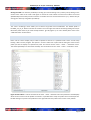
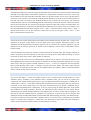
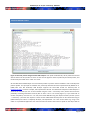
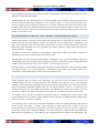
GPR Analyzer v1.23 (Feb. 27th 2012) -‐ MANUAL GPR Analyzer version 1.23 – User’s Manual GPR Analyzer is a tool to quickly analyze multi-‐species microarrays, especially designed for use with the MIDTAL (Microarray Detection of Toxic ALgae) chip. It will read Genepix .GPR files produced by scanner software and perform probe averaging and normalization, infer cell concentrations, and perform internal validation of the results taking advantage of hierarchical probes. CONTENTS Getting started ........................................................................................................................................................ 2 Installation and system requirements ................................................................................................................ 2 Loading a .gpr file. .............................................................................................................................................. 2 Entering metainfromation .................................................................................................................................. 2 Displaying your data ........................................................................................................................................... 3 Changing your normalization probe ................................................................................................................... 6 Working with filters ............................................................................................................................................ 6 Exporting results ................................................................................................................................................. 7 Checking for updates .......................................................................................................................................... 7 For advanced users ................................................................................................................................................. 8 Hierarchy data .................................................................................................................................................... 8 The math behind S/N ratios, total intensity, and normalized mean. ................................................................. 9 Calibration data .................................................................................................................................................. 9 Inferring cell concentrations ............................................................................................................................. 10 The hybridization-‐specific detection limit ........................................................................................................ 11 Disclaimer ......................................................................................................................................................... 11 Frequently asked questions (FAQs) ...................................................................................................................... 12 Page 1 of 12 GPR Analyzer v1.23 (Feb. 27th 2012) -‐ MANUAL GETTING STARTED INSTALLATION AND SYSTEM REQUIREMENTS GPR Analyzer should run on any system (Windows, Linux, Mac) with a recent version of a JAVA runtime environment (JRE). It was tested on Windows 7 64 bit (Java 1.6.0_21) and Mac OS X Snow Leopard (Java 1.6.0_29). Windows users can download a JRE free of charge from Oracle at this address http://www.java.com/en/download/index.jsp. GPR Analyzer does not require any installation. Simply unpack the “.zip” archive into a folder of your choice and double-‐click the” GPRTransformer1.23.jar” file. If you downloaded a bundle specifically for Windows or MacOS, you can also double-‐click on the corresponding “.exe”-‐file or the “.app” bundle instead. Please note that file extensions (the part after the last “.”) may be hidden depending on your system settings. The program should appear on your screen. For the program to work properly, please ensure that you have write access to the directory you chose and do not remove any of the files found here (“caldata.dat”, “hierarchy.xml”, and “settings.ini“). LOADING A .GPR FILE. “.gpr” files are generated by your scanner software. To load one of these files choose “File -‐-‐> Import .GPR”. If you wish to load a different file, choose “File -‐-‐> Import .GPR” again and select a different file. The current data will be discarded and the new data loaded. If you do not have a GPR file available, you can start with a file from “sample data” folder in the GPR tansformer directory. If you have technical replicates you wish to analyze at the same time, you can load additional replicates using the “File -‐-‐> Import replicate .GPR” command. This option will add another “.gpr”-‐file to your current analysis. ENTERING METAINFROMATION When you load a GPR file you will be asked to enter additional information about your sample. These data are necessary in order to calculate estimates for the number of cells present in your sample. The actual calculations are detailed below. If essential fields are left blank, no cell numbers will be calculated and the corresponding column will be blank. The fields required depend on the probe used for normalization and the corresponding formula. By default, the number of Dunaliella cells added prior to the extraction and the volume filtered will be required if you are using the “DunGS02_25_dT_dT” probe for normalization. The total quantity of RNA extracted from your sample, as well as how much was used for your hybridization will be required for standards added to the hybridization buffer. The degree of labeling for your sample is required only if the standard is already labeled and added after the labeling step. Please note that “.” should be used as decimal separator. Data that was entered incorrectly will be highlighted in red when you press “ok”. Should you wish to modify the sample meta information at a later point in time, please select “Tools -‐-‐> Edit sample data” to return to the dialog (see Figure 1). Page 2 of 12 GPR Analyzer v1.23 (Feb. 27th 2012) -‐ MANUAL Figure 1: Dialog for entering sample metadata. It is automatically displayed when loading a .gpr file or can be accessed via the “Tools -‐-‐> Edit sample data…“ menu DISPLAYING YOUR DATA The main display in GPR Analyzer consists of two tables: the top table displaying summaries for each probe (referred to as “Probe table”), and the bottom table containing detailed information about the replicate spots (features) for the currently selected probe (referred to as “Spot table”) (Figure 2). Figure 2: Overview of the interface. The upper table displays probe averages, while the lower table details about the spots (i.e. features) associated to the currently selected probe. This the top table may be customized using the “Tools -‐-‐> Settings” menu Page 3 of 12 GPR Analyzer v1.23 (Feb. 27th 2012) -‐ MANUAL The spot table (the lower one) allows you to examine mean fluorescence (Fmean), mean background (Bmean) as well as the signal / noise ratio and the total signal intensity for each probe. You can also choose to activate or deactivate an individual spot by clicking on the corresponding check box. Only “active” spots will be used for the calculation of the data shown in the probes table. Spots with an Fmean and a Bmean of 0 are deactivated by default. Please note that it is advisable to identify and remove low quality spots already during image analysis, as more information about the context is available. If you find strong differences between spots form different blocks, please re-‐check your image. The columns displayed in the probe table (the upper one) can be customized according to your needs via the “Tools -‐-‐> Settings” menu, where you can select the columns to display in the “Output” section. The information displayed in each column is described below: Figure 3: Tools -‐-‐> Settings dialog. This dialog is used to set the normalization probe, signal to noise ratio, and output options. The list of probes on the right hand side is only available if a “.gpr” file was loaded. All settings are automatically saved if you press “Apply changes” and will remain active even if you restart the program. Species used for calibration (Species): Your calibration file (see below) may contain information relating probe names to species. If this information is available for a probe it will be displayed in this column. Number of spots (Spots): This column displays the number of replicate spots for a probe currently considered for the calculation before the “/”, and the total number spots available for this probe after the “/”. Mean signal/noise (S/N): This is the ratio of the mean signal of a probe and the local background signal. The signal to noise ratio is an important measure to determine if a probe is highlighted or not. A corresponding cut-‐ off can also be set in the “Tools -‐-‐> Settings” menu and will affect the calculation of cell numbers, the hierarchy Page 4 of 12 GPR Analyzer v1.23 (Feb. 27th 2012) -‐ MANUAL check, and color highlighting (see below). As a rule of thumb a signal to noise ratio >= 2 is used as an indication that labeled RNA has bound to your probe. Standard deviation of signal/noise (S/N SD): The standard deviation of the mean signal to noise ratio, calculated for the active replicate spots. Mean total signal (Total): The total signal is used to quantify how much labeled RNA has bound to a probe (and thus was present in your sample. It is used to calculate the normalized signals and to infer cell numbers, as it is not easily affected by differences in the background (noise). Standard deviation of total signal (Total SD): The standard deviation of the mean total signal, calculated for the active replicate spots. Mean normalized signal (Norm.): This is the total signal of the current probe, divided by the signal of the selected normalization probe. The normalized signal should be independent of your scanner settings, the quality of your hybridization, and, depending on when your standard was added, also of the labeling and extraction efficiency (in the case of Dunaliella as a standard). Standard deviation of normalized signal (Norm SD.): The standard deviation of the mean normalized signal, calculated for the active replicate spots. Inferred cell number (Cells/L): This number is an estimate of the cell concentration for a specific species in your original sample (in cells per liter) based on the sample information you have entered and the available calibration data. It is calculated only for probes with a signal/noise ratio greater than your cut-‐off (see Tools -‐-‐> Settings). If your signal to noise ratio is between 1 and your cut-‐off, the program will calculate the number of cells that theoretically would have been necessary to yield a signal corresponding to your cutoff (see below). This number is displayed following the “<” sign, and can be used as a rough indication of your detection limit. Please also consider that the inferred cell numbers may be biased by unspecific signals, differences in the standards, or also by differences in the cellular RNA content of your species. Cell numbers are only calculated if calibration data is available for the current species of interest and the selected normalization probe. Hierarchy check information (Hierarchy): This column displays the results of the “Hierarchy check”. For all probes that are above the selected signal to noise cutoff, the program will check if any higher level probes are present on the microarray, and if so if these probes are above your cutoff as well. If all higher level probes are also above your threshold the result will be “PASS” and the probes that were tested will be listed in parentheses. If e.g. a species-‐specific probe is above your threshold, but the corresponding genus probe is not, the result of the “Hierarchy check” will be “FAIL” and lists of higher level probes that either passed or failed will be given in parentheses. Information about the hierarchical structure of the probes is saved in the hierarchy file (see below). If no higher level probe is present on the array this field will be left blank. If the hierarchy file indicates a higher level probe that was not found on the array, the result will be “Missing”, and the probe(s) not found will be given in parentheses. Color highlighting: To make it easier for you to get an overview over your data, GPR Analyzer uses a green background to highlight probes that have a signal to noise ratio above your cutoff and that have not failed the hierarchy check (either no higher level probes were available, or all higher level probes were also above the threshold). Probes with a signal to noise ratio above the threshold that have failed the hierarchy check are marked in yellow. Probes below the cutoff have a white background. Page 5 of 12 GPR Analyzer v1.23 (Feb. 27th 2012) -‐ MANUAL Sorting the table: You have the possibility of sorting your data according to any column just by clicking on the column name. Click on the same name again to reverse the order. Please note that cell numbers are sorted alphabetically because they contain a mixture of numbers and non-‐numerical characters (“<”). Another way of sorting your data is by using filters (see below). CHANGING YOUR NORMALIZATION PROBE The “Tools à Settings” menu allows you to choose any probe from normalization. The default probe is DunGS02_25_dT_dT. Please note that the “Probes” list on the right hand side of the Settings dialog will only be filled with probe names if you have already loaded a .gpr file (Figure 3). For more details please refer to the “calibration data” section below. WORKING WITH FILTERS Filters can be used to display only a subset of probes of interest in a specified order. There are two ways loading a filter into the program. One option is to load a filter from a plain text file listing the name of each probe you want to display in a separate line, each. This is done via the “Tools -‐-‐> Filter -‐-‐> Load filter” menu. The second possibility is to edit a filter manually. This can be done via the “Tools -‐-‐> Filter -‐-‐> Edit filter” menu. Figure 4: Filter editor. It can be accessed via the Tools -‐> Filter -‐> Edit filter menu and provides a text field (left) which can be used to enter all probes of interest in a specified order. Only one probe can be entered per line. Double clicking on a probe in the probe list on the right will insert the probe at the current cursor position. Page 6 of 12 GPR Analyzer v1.23 (Feb. 27th 2012) -‐ MANUAL The filter editor (Figure 4) consists of a large text field which can be used to enter the list of probe names either manually or by copy-‐pasting it from another application. A complete list of probes found in your current .gpr file is available on the right hand side of the filter editor if a .gpr file is loaded. You can insert a probe name at the current cursor position in the text field, simply by double clicking on the probe in the list. Please make sure that only one probe is entered per line. Multiple probes per line or probes not found in your .gpr file will be omitted. Another option is to automatically generate a filter based on the probes (and the order of the probes) found in your hierarchy file. This is done by pressing the “Import from hierarchy” button in the filter editor. The filter you have loaded or created will automatically be activated (unless you choose cancel in the editor). It can later be deactivated and reactivated using the “Tools -‐-‐> Filter -‐-‐> Deactivate filter” and the “Tools -‐-‐> Filter -‐-‐> Activate filter” menus. You can also save your current filter for later use using the “Tools -‐-‐> Filter -‐-‐> Save filter” command from the main menu. EXPORTING RESULTS The results of your current analysis (the probes table) can be exported either by using the “File -‐-‐> Export .TXT” command or using the “Copy” button in the top right corner of the program. Using either option, a tap-‐ separated text will be generated and either saved as a file or copied to your system’s clipboard. This tab-‐ separated text can then be opened by or pasted to other application such as Excel or OpenOffice Calc for further analysis. The exported data will comprise all columns currently visualized in the probe table. Any sorting or selection of probes using filters will be considered for the export, but sorting of the probe table by clicking on column names has no effect on the order in which probes are exported. Please note that the current version of GPR Analyzer supports only an export in the plain text format. Thus color highlighting can presently not be included. In addition, for use with spreadsheet programs such as Excel, please ensure that your system’s decimal separator is set to “.” or that you change the decimal separator option in GPR Analyzer under “Tools -‐-‐> Settings” to match that of your system. This option affects only the way numbers are exported, not the way they are displayed within the program, which is determined by the version of JAVA running on your machine. CHECKING FOR UPDATES You can use the “About -‐-‐> Check for updates” option to see if a newer version of GPR Analyzer or of the calibration data is available. If new calibration data is available online, you can choose to update your “caldata.dat” file without restarting the program. Your old calibration file will be backed up as “caldata.bak” or “caldata.bak.n”, where “n” is a number increasing with each backup found. If the update fails, e.g. because the connection to the server breaks down, you can either manually restore your previous calibration file by renaming the latest backup file to “caldata.dat”, or you can retry running the update again later. If you update your calibration file while analyzing a GPR file, the metadata you have entered for your sample will be overwritten by the default metadata defined in the calibration file. In order to update the main program, you will need to visit the indicated web-‐site, download, and unpack the contents of the zip file into your GPR Analyzer directory manually. GPR Analyzer comes bundled with default settings, hierarchy, and calibration files. If you wish to keep your current files when updating, choose “no” when you are prompted by your operating system to overwrite the “settings.ini”, ”caldata.dat”, and “hierarchy.hir” files. Please note that checking for updates and the automated update requires an active network connection. Page 7 of 12 GPR Analyzer v1.23 (Feb. 27th 2012) -‐ MANUAL FOR ADVANCED USERS HIERARCHY DATA Figure 5: Hierarchy viewer integrated into GPR Analyzer. Each probe is followed by a list of probes that should also be active if the first probe is. If this is not the case the signal for the first probe may be a false positive, and the hierarchy check will return “FAIL” as a result. As described above GPR Analyzer uses hierarchical probes to perform internal validation and to identify false positive probes. This principle of validation has previously described and been implemented by Metfies et al. (2008, Mol. Ecol. Res. 8:99-‐102). GPR Analyzer supports the same XML format for hierarchy files as Phylochipanalyzer, as well as a simpler, tab-‐separated text format. The default hierarchy file for GPR Analyzer is stored in the “hierarchy.hir” file. It can be viewed using the “Tools -‐-‐> Hierarchy” menu, where there is also the possibility of loading alternative hierarchy files in either .xml or .hir format (Figure 5). If you would like to convert a Phylochip “.xml” file to a “.hir” file, first load the XML file using the “Import hierarchy” button (“Tools -‐-‐> Hierarchy…”) and then the “Export as .hir file” button. XML-‐based hierarchy files can be customized using an (XML-‐enabled) text editor or Phylochip Analyzer; tab-‐separatated “.hir” files can be edited e.g. using a text editor or a spreadsheet application such as Excel. Each line contains the name of a probe on the chip as well as Page 8 of 12 GPR Analyzer v1.23 (Feb. 27th 2012) -‐ MANUAL list of all higher level (parent) probes. All probe names are separated by tabs. Empty lines or comments starting with “##” are ignored by GPR analyzer The advantage of the “.hir” as opposed to the “.xml” file is flexibility. Let’s assume you have two probes (p1 and p2) on the same hierarchical level targeting the same organisms. Using a “.hir” file, you can then define p1 as parent to p2 and at the same time p2 as a parent for p1. This way p1 and p2 will only pass the hierarchy check if both are above the cut-‐off. Using the Phylochip xml format, you can only define either p1 as parent for p2 or p2 as a parent for p1, but not both. This way one of the two probes may pass the hierarchy check, even if the other is not above the cut-‐off. THE MATH BEHIND S/N RATIOS, TOTAL INTENSITY, AND NORMALIZED MEAN. These three parameters are the basis of all analyses. Each of these values is calculated from a number of values extracted for each spot from different columns of the GPR file. They are “B635 Mean”, “F635 Mean”, and “Dia.” and correspond to the mean fluorescence at 635 nm for the spot, the mean fluorescence of the local background, and the diameter of the spot, respectively. The “Name” column is used to name probes and group identical probes for averaging. The signal to noise ratio is calculated as “F635 Mean”/ “B635 Mean”. Mean and standard deviation are calculated for the ratios of all active probes with identical names. The total signal intensity is calculated as (“F635 Mean”-‐ “B635 Mean”)*”Dia.”*”Dia.”/4*3.14159, the latter part corresponding to the area of the spot. Mean and standard deviation are calculated for all total signal intensities of active probes with identical names. Total intensities < 0 are automatically set to 0. Normalized signals are calculated by dividing the total signal intensity calculated for each spot by the average total signal intensity of the probe designated as normalization probe. Mean and standard deviation are calculated for all normalized signals of active probes with identical names. CALIBRATION DATA Default calibration data are stored in the “caldata.dat” file and used to infer cell numbers based on the normalized signals, but you can temporarily load other calibration files using the “File -‐-‐> Load alternative calibration” menu. GPR Analyzer calibration files are commented, tab-‐separated text file which can be edited in common spreadsheet applications (please note that the decimal separator must be “.”). Empty lines and comments starting with “#” are ignored by the program. The calibration file consists of four sections: “Version”, “Formulas”, “Factors”, and “Data”, each of them is started by and “!” followed by the name of the section. The “Version” section consists of a single line containing “!Version=” followed by the version number of the current calibration file. If you have a costume calibration file and you wish to disable automatic updates please set the version line to “!Version=noupdate”. The “Formulas” section contains one line for each normalization probe with available calibration data, followed by five columns with “TRUE” or “FALSE” values depending on which blocks of the formula to infer cell concentrations (see “Inferring cell concentrations”) should be activated. The order of columns is indicated in the file by a comment and is “Degree of labeling”, “Dunaniella cells spiked”, “Ratio of total extracted RNA and RNA used for the Hybridization”, “Liters filtered”, and “ng of positive control added to the hybridization”. The Page 9 of 12 GPR Analyzer v1.23 (Feb. 27th 2012) -‐ MANUAL last column contains a label for the values calculated with the formula, e.g. “Cells”, “Cells/L”, or “ng target RNA”. The “Factors” section contains information about your calibration curves. The first column indicates the name of the factor described, the second column contains the corresponding value. The factors considered are “DOL” (Degree of labeling for your calibration curve), “DunCell” (the number of Dunaliella cells added for your calibration curve), and “ngPC” (ng of positive control added for your calibration curve). Not all of the factors will be used for all calculations depending on the formulas defined in the “Formulas” section. Please note that only one value per factor can be entered for all calibration curves. If you are preparing your own calibration file and if some calibration curves were carried out differently from others, these will have to be normalized to standard conditions first. The “Data” section contains the actual calibration information for an individual probe. The first column indicates the name of the probe for which the calibration data is valid, the second the species used for this calibration curve. The following columns indicate the calibration factors for each of the possible normalization probes in the same order as defined in the “Formulas” section. The calibration factor is the slope of a calibration curve plotting the normalized signal against the number of cells of the present species in a sample. It is assumed that all calibration curves cross the x-‐axis at x=0 (i. e. that no signal is obtained if no RNA is hybridized). INFERRING CELL CONCENTRATIONS The most important step for inferring cell numbers is to divide the normalized signal obtained for a probe of interest using a given normalization probe by the normalization factor for the same probe of interest and same normalization factor in the calibration file. Since this factor corresponds to a slope of a calibration curve plotting normalized signals against cell numbers, this simple division will yield a first estimate of the cell number. A number of different components (see “Formulas” section in the calibration file) can be added to this formula to take into account different experimental setups and different probes used for normalization. Volume filtered The first factor is the volume filtered for your extraction. This will allow the calculation of cell concentrations rather than absolute cell numbers, by dividing the inferred cell number by the volume (“Liters” in the “Formulas” section). Dunaliella cells added The default way of normalizing in the MIDTAL Project is by adding a defined number Dunaliella cells to the field samples and by using the signal obtained from a Dunaliella specific probe (DunGS02_25_dT_dT). Since everything that is done with your sample is also done with the added Dunaliella cells, no additional factors need to be considered with this method. However it is necessary, that the calibration curves and your samples were spiked with the same number of Dunaliella cells added. If this was not the case, this can be corrected for, and this is why it is necessary to add the number of Dunaliella cells added both to your sample information and to the calibration data (“DunCell” in the “Formulas” and “Factors” sections). If “DunCell” is activated in the Formulas section, your inferred cell number will be divided by the number of Dunaliella cells added in the calibration curves, and multiplied by the number of Dunaliella cells added to your sample. Quantity of PC used Page 10 of 12 GPR Analyzer v1.23 (Feb. 27th 2012) -‐ MANUAL If DNA-‐ or RNA based standards are used for calibration (PC, positive control), the same quantity of standard needs to be added to your sample and to the samples used to generate the calibration curve. If this was not the case, this can be corrected for via the “ngPC” option. If “ngPC” is activated in the “Formulas” section, your inferred cell number will be divided by the quantity of standard added in you calibration curves, and multiplied by the quantity of standard added to the sample. Mathematically this option is identical to the “Dunaliella cells” option, but the extraction efficiency is not considered. RNA ratio If you are calibrating your array with a standard you have added after taking an aliquot of your sample for the hybridization two additional pieces of information need to be considered: how much RNA was extracted from your sample, and how much of that was spiked with your standard. Both pieces of information can be entered in the “Tools – Edit sample information…” menu. If “RnaRatio” is selected in the “Formulas” section your inferred cell number will be multiplied by your total RNA extracted, and divided by the amount of RNA used for the hybridization Degree of labeling If your standard (positive control) is already labeled, and added after the labeling step, you can consider differences in the labeling efficiency (degree of labeling, DOL) for your sample and for the samples used in the standard curve. The DOL is calculated as [0.34 ng/pmol] * [Cy5 Concentration in the labeled extract in pmol / µl] / [RNA concentration in the labeled extract in ng/µl] * 100%. This corresponds to the proportion of labeled bases in your sample. If “DOL” is activated, your inferred cell number will be multiplied with DOL in your calibration curves and divided by the DOL in your sample. In the calibration file that comes with the program, all DOLs were normalized to 2%. THE HYBRIDIZATION-‐SPECIFIC DETECTION LIMIT In some cases probes may have signal to noise ratios only slightly below your detection limit. In such cases it is difficult to tell if algae of the species of interest are present in the sample or not, especially considering that the detection limit may vary strongly depending on the quality of the hybridization and the quantity of material hybridized. To help users evaluate negative results, hybridization-‐specific detection limits are estimated. These calculations are essentially the same as those to calculate cell numbers, except that they are based on a hypothetical total signal, which is the hypothetical signal intensity that would have yielded a signal to noise ratio corresponding to the cutoff. This hypothetical total signal is calculated based on the local background of the relevant probes, but assuming the spot diameter set for the probe used for normalization. The diameter of the normalization probe is used to avoid problems that may occur the scanner software is set to detect spot diameters automatically, but fails to do so correctly when the signal for the probe of interest is low.The inferred detection limits are shown in GPR Analyzer after a “<” sign for probes with available calibration data and a signal to noise ratio below the detection limit and above 1. DISCLAIMER Please note that the calculated cell numbers and detection limits are only very rough approximations of what may be found in a field sample. They will depend on the cellular RNA content in your sample, and may vary significantly, depending on how many factor are considered in the calculations. Most importantly cell numbers will be under-‐estimated if probes are saturated. Page 11 of 12 GPR Analyzer v1.23 (Feb. 27th 2012) -‐ MANUAL FREQUENTLY ASKED QUESTIONS (FAQS) If you are experiencing problems with GPR Analyzer, please write an email to [email protected]. I will try to answer your question, or, in case of a bug report, to fix the problem. Why is the cell number column empty? The reason for this is usually that no calibration data is available for the probe used for normalization. Please ensure that the “caldata.dat” file is present in the GPR Analyzer directory, and select a probe with calibration information to normalize your data. Please also enter all the necessary metadata for your hybridization. Calibration data is currently not available for all species / probes. Page 12 of 12