Download Application Note 30

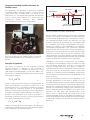
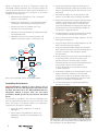
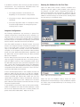
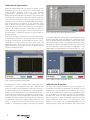
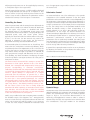
APPLICATION NOTE
Computer Controlled Variable
Attenuator for Tunable Lasers
30
Technology and Applications Center
Newport Corporation
Computer-Controlled Variable Attenuator for
Tunable Lasers
This application note describes a closed loop, computercontrolled, variable attenuator (Figure 1) for the control of
output power from a tunable laser. It is based on the
combination of a 1/2 wave-plate and a polarizer. The algorithm
used to control power operates in a closed loop with
Proportional
Integral
Derivative
(PID)
feedback,
compensating for slow changes in output power.
Beam Sampler 1
Detector
Beam Sampler 2
To
Experiment
From
Laser
Glan-Laser
Polarizer
Beam Dump
Spectrometer
Motorized Rotation
Stage with 1/2 Wave-Plate
Figure 2. Block diagram of the computer controlled attenuator.
Figure 1. The computer-controlled variable attenuator. The setup consists of a
detector, a single channel power meter, a Glan-laser polarizer, a 1/2 wave-plate
mounted in a motorized rotation stage, two beam samplers, a spectrometer
and a PC
Principle of Operation
The theory of operation for the computer-controlled
variable attenuator is identical to that presented in
Application Note 26 - Variable Attenuator for Lasers
(www.newport.com/AppsNote26). It is based on Malus’s law.
The intensity, I, of linearly polarized light that passes through
the polarizer is given by
I = I o cos 2 θ
(1)
where Io is the input intensity and θ is the angle between the
beam’s initial direction of polarization and the axis of the
polarizer. Rotation of a 1/2 wave-plate mounted in a rotational
stage allows for continuous rotation of the polarization
direction of the linearly polarized light. Thus, combined with
a polarizer, it provides variable attenuation according to (1).
Rotation of the wave-plate by an angle of ϕ results in a
polarization rotation by an angle of 2 ϕ, thus the intensity at
the output of the attenuator is given by,
I = I o cos 2 2ϕ
For the manual variable attenuator, the power is measured
directly at the output of the attenuator for each wavelength
and set accordingly by rotating the 1/2 wave-plate. In contrast,
the computer-controlled closed loop attenuator sets and
maintains the power by positioning the 1/2 wave-plate based
on a feedback signal from a photo-detector. The photodetector can exhibit a strong dependence on wavelength
(www.newport.com/818Series). This chromaticity becomes
significant when the tuning range is large. Consequently, a
spectrometer is incorporated into the setup, which provides
real-time information about the laser’s wavelength, thus
taking advantage of the photo-detector’s precise wavelength
calibration. This is especially important when the laser power
needs to be held constant while scanning wavelength.
Depending on the choice of components, the attenuator
is suitable for laser wavelengths ranging from 400 nm to 1100
nm, and average powers from 1 nW up to 20 Watts (500
Watts/cm2 damage threshold). This device is capable of
attenuating light by a factor of 1000 while still maintaining an
error of less than 10%. The algorithm used to control power
operates in a closed loop with PID feedback, compensating
for slow changes in output power within the bandwidth of the
device (> 500 ms).
Prior to the wave-plate, a fraction (1%-10% depending on the
incoming polarization) of the beam is picked off by the
first beam sampler and sent to a spectrometer. The remainder
of the beam travels through the 1/2 wave-plate and Glan-laser
polarizer. The attenuated output from the polarizer passes
through the second beam sampler where a fraction of the
beam is directed towards the detector at an angle of 10º
relative to the main beam. The rejected portion of the
beam is sent to a beam dump. The overall losses of the
attenuator depend strongly on the degree of polarization, as
well as the polarization state. However, if the incoming beam
is fairly well polarized in the P-plane, the overall losses are
below 10%.
(2)
where ϕ is the azimuth of the /2 wave-plate. The full range of
attenuation is realized over 45º of rotation. The block diagram
for the attenuator is illustrated in Figure 2.
1
1
Figure 3 illustrates the flow of information within the
automated variable attenuator. The red arrows depict the
route of the laser through the various optical components as
described above. The CPU acts as the “brain” of the system
and plays the following role:
1. Determines the angle/phase of the 1/2 wave-plate
relative to the polarizer.
2. Monitors the wavelength, λ, from minispectrometer
and updates the power meter wavelength setting.
3. Monitors the power of the beam out of the
attenuator via the power meter.
4. Determines the error between the output power and
the requested power.
5. Minimizes this error using a PID algorithm, and
updates the rotation stage to a new position, ϕ.
Minispectrometer
4. Move the base-plate into the final position and
secure it to the table using the clamps provided.
5. Temporarily arrange the wave-plate, polarizer, beam
samplers, spectrometer assembly and detector as
shown in Figure 4. Take care to ensure that the
angle formed between the primary beam path and
the beam path from the second beam sampler to
the detector is approximately 10º.
6. Secure the detector and the spectrometer assembly
to the base-plate and remove all other optics.
7. Turn on the laser and insert beam sampler 1 into the
beam path (see Figure 4).
8. Using the tip/tilt, direct the reflected beam onto the
fiber of the spectrometer assembly.
Laser
Fraction
of Beam
3. Turn the base-plate right side up and position it
underneath beam path. Verify that the center of the
beam is approximately 46 mm above the top of the
base-plate.
9. Insert the wave-plate and polarizer into the beam
path. Adjust the position such that the beam passes
through the center of the wave-plate. Secure
the wave-plate.
Beam
Sampler
λ
ϕ
Requested
Power
CPU
Polarizer
λ
Signal
Proportional to
Total Power
Power
Meter
1/2
Wave-Plate
Rotation
Fraction
of Beam
Dump
Beam
Sampler
Experiment
Figure 3. Flow chart describing operation of the automated attenuator
Assembling the Attenuator
10. Rotate the polarizer such that the transmitted light
is minimized. Next, fine tune the angle of the
polarizer relative to the beam path to further
minimize transmission. Secure the polarizer. Rotate
the polarizer such that the tick marks lie
in the horizontal plane (P-polarization relative
to beam sampler 2).
11. Insert beam sampler 2 into the beam path. Use the
tip/tilt to direct the reflection of the uncoated
surface onto the face of the detector. Take care to
ensure that the second reflection from the coated
surface is not incident on the detector.
12. Position Beam Dump to capture rejected beam.
Secure to base-plate.
WARNING-Radiation emitted by laser devices can be
dangerous to the eyes and appropriate precautions must
be taken when they are in use. Only individuals who are
adequately trained in proper laser use and safety
procedures should operate the laser devices described
herein.
The instructions provided in this note are intended for use
with the Spectra-Physics Mai Tai® laser. For use with other
lasers, the height of the device needs to be adjusted to
correspond to the height of the beam.
1. Mount all optical components as shown in
Appendix 1.
2. Attach three 2-inch pedestals as well as the
SMC100CC controller to the underside of the
base-plate.
2
Figure 4. Automated variable attenuator. The red line illustrates the beam path.
The numbered optics correspond to: 1-beam sampler, 2-1/2 wave-plate and rotation
stage, 3-Glan-laser polarizer, 4-beam sampler, 5-918D-UV-OD3 photo-detector
and 6-mounted fiber connected to minispectrometer.
It should be noted that there are many possible attenuator
configurations. The configuration described above was
chosen because it offers several advantages:
1. The output polarization can be either S or P
depending on the orientation of the polarizer.
2. The power on target is directly sampled rather than
calculated.
Running the Software for the First Time
Open the SMC Power Control software (available from
Newport’s pre-sale support ((800) 222-4640). Upon opening
the program, the Data screen is displayed (see Figure 5).
Select the Parameters tab (see Figure 6). Under this tab are
the control settings for this device, including the hardware
addresses and the settings for the PID control. Initially, leave
the PID settings to the default values.
3. The control algorithm makes no assumptions about
the relationship between the wave-plate position
and the power on target.
Computer Configuration
The following requirements are necessary to operate this
software. The processor should be at least a Pentium 4 (or
equivalent) with 512 MB of RAM. The hard drive should have
at least 50 MB of storage space available and have LabVIEW
Run-Time Engine 8.2 installed. The operating system tested
with this device is Windows XP Professional Edition.
Once the variable attenuator is aligned, connect the power
meter to the computer through the USB port located on the
rear of the power meter. Connect the motorized rotation
stage to the SMC100CC controller. Connect the SMC100CC
controller to the computer using the RS232 cable provided.
Install the Power Meter, Minispectrometer, SMC100CC and
the SMC Power Control software using the disks provided.
Reboot the computer.
Figure 5. SMC Power Control Data screen
Run the SMC program from the Start Menu. Make sure the
stage is properly configured and sent to the home position.
Note the address settings in the Configuration Panel. Close
the SMC100CC program. After successful completion of this
step, a green LED should be illuminated on the SMC100CC
controller. If it is not, the SMC100CC controller is not properly
configured and the device will not function. If this is the case,
consult the SMC100CC User’s Manual.
Connect the Minispectrometer to the computer through the
USB port. Make sure that the laser is on and the “sampled”
beam is hitting the Minispectrometer fiber. Open the TraqPro
software provided and acquire data. Make sure that the
spectrometer is capable of “seeing” the laser light. If the laser
saturates the spectrometer, insert a diffuser into the beam
path or decrease the integration time until the laser no longer
saturates the spectrometer.
Figure 6: SMC Power Control Parameter window.
Make sure that the hardware settings match the values
displayed in the Device Manager. If they are different, update
the values using the Reinitialize Key to the settings in the
Device Manager.
In the Windows Control Panel, open up the System window.
Under the Hardware tab, select the Device Manager. Under
the Ports tab, determine which ports are being used by the
power meter and the SMC100CC. Make note of this.
3
Calibrating the Spectrometer
Select the Spectrometer tab (see Figure 7). Initially, set the
integration time to 50 ms and run the spectrometer. The
graph displays intensity (counts) vs. pixel number.
Wavelength is calculated from a calibration file, and
displayed in the Data window (see Figure 5). Turn on the laser
and observe the signal. If the spectrum is below the level of
noise, increase the integration time. Note that increasing the
integration time also decreases the bandwidth of this device,
thus slowing down the operation of the attenuator. More
likely, it will be the case that the spectrometer is saturated
(more than 55000 counts). If this is the case, the integration
time can be reduced; however, neutral density filters as
well as diffusers (cosine correctors) can also be inserted into
the beam path to reduce the amount of light incident on
the spectrometer.
If the laser is tunable, scan the laser across the tuning range
and observe the spectrum. It is important that the spectrum
be above the noise level at all wavelengths. Again, using a
combination of the integration time along with the
appropriate filters, make sure that the laser spectrum is
above the level of the noise, but below saturation for the
necessary wavelength range.
Figure 7: SMC Power Control Spectrometer window.
The SMC Power Control software comes preloaded with a
wavelength vs. pixel calibration file. This calibration will
suffice for power control applications since the accuracy of
the device need only be on the order of a few nanometers.
However, if the spectrometer is to be used quantitatively, it
may be necessary to manually re-calibrate the spectrometer.
If this is the case, collect the spectrum of the known source.
Determine the pixel number of the peaks using the intensity
vs. pixel graph. Select the Calibrate Spectrometer key (see
Figure 7). A screen with two columns and a graph of pixel
number vs. wavelength will appear (see Figure 8). Deselect
4
Figure 8: SMC Power Control Wavelength Calibration window.
the default calibration and select the Overwrite button. In the
columns provided, enter the calibration wavelengths along
with the corresponding pixel numbers. Using the bar, select
the order of the polynomial (1-5) needed to describe the data.
The graph will display the updated calibration values along
with the calibration curve. Ultra-precise calibration is not
required with this spectrometer since the resolution is ~1nm.
Figure 9: SMC Power Control Auto-Calibrate window.
Calibrating the Wave-plate
The heart of the variable attenuator is the 1/2 wave-plate. It is
responsible for rotating the polarization of the light. It is not
required that the wave-plate be mounted in the rotation
stage in any specific way; instead, the program will recognize
the angle/phase of the wheel through the auto-calibrate
function. First, select the Auto-Calibrate tab from the main
panel (see Figure 9). Enter the number of points to be used
in the calibration. Twenty points is a good starting value;
however, more points can be added depending on the
required accuracy. Press the Start button. The rotation stage
will progressively rotate over 90º. The graph displays intensity
vs. wave-plate angle as the stage rotates.
After the stage finishes rotating, a solid line will be displayed
on the graph derived from the best fit to Equation 2. This
curve is used to set the high and low position limits for the
rotation stage as well as determine the parameters used to
calculate the intensity of the laser prior to attenuation.
Controlling the Power
After the spectrometer and the wave-plate are calibrated, the
power control is ready to run. Select the Data tab. Make sure
that the Open Loop button is disabled and enter
the desired power in the Requested Power control and
select the Start Power Control button. The graph displays the
requested power (red) and actual power (white).
Typically, the white line tracks the red line within a few steps.
If this is not the case, the PID controls may need to be
adjusted. A reference for PID tuning can be found at
http://www.controleng.com/article/CA307745.html.
As mentioned earlier, the software runs in closed loop. This
means that the 1/2 wave-plate is continuously dithering, which
may adversely affect some experiments. If this is the case, the
user has the option to open the loop by selecting the Open
Loop button. When the Open Loop button is selected, all
gains (proportional, integral and derivative) are set to zero,
thus disabling any wheel movement. Deselecting the Open
Control Loop button (see Figure 5) returns all of the gains to
their previous values.
The Power Control software will also attempt to correct slow
fluctuations in laser output. Because of this, if the laser is
blocked, the 1/2 wave-plate will compensate by moving into a
position corresponding to maximum transmission.
Unblocking the beam will then temporarily deliver full power
on target until the wave-plate has time to respond. This may
result in optical damage to components or a sample
positioned after the attenuator. To prevent this, a safety
feature is built into the PID loop. If the laser power fluctuates
by more than a user specified percentage, the software
automatically opens the loop. When this happens, the error
is logged and the user can reset the loop by deselecting the
Open Loop button. The default percentage setting is 50%,
but this value is free for the user to modify under the
Parameter tab. When operating at attenuation levels higher
than 100 times, care must be taken to block the scattered
light from the detectors. In this case, it is also recommended
to turn the safety feature off (see Figure 6).
Finally, it is possible for the user to request powers outside of
the available range. If this happens, the 1/2 wave-plate will
move to its limit and stop. The power indicator will flash red
and an out-of-range error will be logged. It is not necessary
to reset this error. Simply command the attenuator back
into the appropriate range and the indicator will return to
the normal color.
Polarization Control
As mentioned earlier, one of the advantages to this specific
configuration of the variable attenuator is that the output
polarization can be either horizontal or vertical depending on
the orientation of the polarizer. Changing the polarization or
the angle of the beam sampler after the polarizer will result in
a slight systematic error in the output power. To compensate
for this, the scaling factor in the parameter window can be
altered. The default setting is 0.042 corresponding to a
Fresnel reflection at 10º from a BK7 substrate at 800 nm,
P-polarization. At this angle, the Fresnel reflection has
minimal wavelength dependence, thus allowing the source to
be wavelength tunable without a significant impact to the
attenuator’s performance. However, if the angle or
polarization state is significantly modified, the scaling factor
must be altered to compensate for these modifications. Table
1 lists the scaling factor as a function of wavelength and angle
for both S-(top) and P-(bottom) polarization.
In general the output polarization can be set in any direction
by adjusting the azimuth of the polarizer. The scaling factor
should be adjusted accordingly.
Table 1: Scaling factors at various wavelengths and angles.
o
7
o
9
o
11
o
13
o
15
o
S/P
5
700 nm
0.044
0.043
0.045
0.043
0.045
0.042
0.046
0.042
0.047
0.041
0.048
0.040
750 nm
0.044
0.043
0.045
0.043
0.045
0.042
0.046
0.042
0.047
0.041
0.048
0.040
800 nm
0.044
0.043
0.045
0.043
0.045
0.042
0.0 46
0.041
0.047
0.041
0.048
0.039
850 nm
0.044
0.043
0.044
0.043
0.045
0.042
0.046
0.041
0.047
0.040
0.048
0.039
900 nm
0.044
0.043
0.044
0.042
0.045
0.042
0.046
0.041
0.047
0.040
0.048
0.039
950 nm
0.044
0.043
0.044
0.042
0.045
0.042
0.046
0.041
0.046
0.040
0.048
0.039
1000 nm
0.044
0.043
0.044
0.042
0.045
0.042
0.045
0.041
0.046
0.040
0.047
0.039
Dynamic Range
The dynamic range of the attenuator can be thought of as the
difference between the maximum and minimum achievable
powers. The stated dynamic range is 103; however, dynamic
ranges as high as 105 have been demonstrated in our
Technology and Applications Center. In order to achieve a
dynamic range this high, two important factors must be taken
into consideration: stray light incident on the reference
5
detector must be minimized and the incoming light must be
highly polarized. If a higher dynamic range is required, it is
necessary to include a second polarizer just before the
attenuator. To shield the reference detector from stray light,
place an iris attached to a tube directly in front of the
detector.
Status Log
The SMC Power Control software logs all generated errors,
time stamps them, and records the errors to file. The Status
Log window (Figure 10) allows the user to monitor any
generated errors while the program is operating.
Figure 10: SMC Power Control Status Log window.
Exiting the Program
To exit the program, simply hold down the Quit button until
the program closes. It is preferable to use the Quit button
since all of the devices are properly closed when exiting the
program this way. Repeatedly closing the program by other
means may result in computer instability.
6
Appendix1: Pictures of Mounted Optics
1.
Beam Sampler
2.
Rotation Stage and 1/2 Wave-plate
3.
4.
5.
6.
7.
Polarizer
Beam Sampler
Photo-detector
Fiber connector to spectrometer
Beam Dump
7
Newport Corporation
Worldwide Headquarters
1791 Deere Avenue
Irvine, CA 92606
(In U.S.): 800-222-6440
Tel: 949-863-3144
Fax: 949-253-1680
Email: [email protected]
Visit Newport Online at: www.newport.com
This Application Note has been prepared based on development activities and experiments conducted in Newport’s Technology
and Applications Center and the results associated therewith. Actual results may vary based on laboratory environment and setup
conditions, the type and condition of actual components and instruments used and user skills.
Nothing contained in this Application Note shall constitute any representation or warranty by Newport, express or implied,
regarding the information contained herein or the products or software described herein. Any and all representations,
warranties and obligations of Newport with respect to its products and software shall be as set forth in Newport’s terms and
conditions of sale in effect at the time of sale or license of such products or software. Newport shall not be liable for any costs,
damages and expenses whatsoever (including, without limitation, incidental, special and consequential damages) resulting from
any use of or reliance on the information contained herein, whether based on warranty, contract, tort or any other legal theory, and
whether or not Newport has been advised of the possibility of such damages.
Newport does not guarantee the availability of any products or software and reserves the right to discontinue or modify its
products and software at any time. Users of the products or software described herein should refer to the User’s Manual and other
documentation accompanying such products or software at the time of sale or license for more detailed information regarding the
handling, operation and use of such products or software, including but not limited to important safety
precautions.
This Application Note shall not be copied, reproduced, distributed or published, in whole or in part, without the prior written
consent of Newport Corporation.
Copyright ©2007 Newport Corporation. All Rights Reserved.
Newport Corporation, Irvine, California, has
been certified compliant with ISO 9001 by
the British Standards Institution.
MM#90000090
DS-12065