Download HEWLETT PACKARD 8569B SPECTRUM ANALYZER

rhO-
HEWLETt
a:~ PACKARD
OPERATION AND SERViCE MANUAL
8569B
SPECTRUM ANALYZER
Includes Options"OOl and 002
SERIAL NUMBERS
This manual applies directly to HP Model 8569B
Spectrum Analyzers having serial prefix number
2244A.
For additional important information about serial
numbers see INSTRUMENTS COVERED BY
MANUAL in Section I.
volume 1
GENERAL INFORMATION
INSTALLATION AND OPERATION VERIFICATION
OPERATION
CopyrIght © 1982,HEWLETT·PACKARD COMPANY
1424 FOUNTAIN GROVE PARKWAY, SANTA ROSA,CALIFORNIA, 85404, U.S.A.
MANUAL PARTNO. 08588-10032
Prtnted: December 1182
Scans by ARTEK MEDIA =>
Contents
Model 8569B
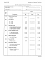
CONTENTS
Section
II
Page
GENERALINFORMATION
1-1. Introduction
1-3. Description
1-9. Manual0rganization
1-11. Specifications
1-13. Safety Considerations
1-18. Instruments Covered By Manual. . . . . . .
1-27. Options.......................
140. Accessories Supplied
142. Equipment Available
149. Recommended Test Equipment. . . . . . .
1-1
1-1
1-1
1·1
1·1
1-2
1-3
1-3
14
14
14
INSTALLATION AND OPERATION
VERIFICATION
2-1.
Introduction
2·1
2-1
Page
Section
2-3.
2-5.
2-25.
2-31.
2-33.
2-34.
2-35.
2·36.
III
Initial Inspection
2-1
Preparation for Use
2·1
Storage and Shipment
2-7
Operation Verification
2-7
Operational Check
2·8
Tuning Accuracy
2-8
Frequency Span Width and
Resolution Bandwidth
Accuracy
2-10
Amplitude Accuracy . . . . . . . . . . . . . 2-12
OPERATION
3-1. Introduction
34.
Routine Maintenance
3-1
3-1
3-1
LIST OF ILLUSTRATIONS
Figure
Page
1-1. HP Model 8569B Spectrum Analyzer with
Accessories Supplied . . . . . . . . . . . . . . . . . . 1-0
1-2. Typical Serial Number Plate . . . . . . . . . . . . . . 1-3
1-3. Service Accessories Package. . . . . . . . . . . . .. 1-12
2-1. Line Voltage Selection with Power
Module PC Board
24
Figure
Page
2-2. Attaching Rack Mounting Hardware
and Handles. . . . . . . . . . . . . . . . . . . . . . . . 2-5
2-3. Packaging for Shipment Using Factory
Packaging Materials
2-6
24. Operation Verification Test Setup
2-9
2-5. Span Width Accuracy Measurement
2-11
LIST OF TABLES
Table
Page
1-1. HP Model 8569B Specifications
1-5
1-2. HP Model 8569B Supplemental
Characteristics . . . . . . . . . . . . . . . . . . . . . . 1-8
1-3. Recommended Test Equipment. . . . . . . . . .. 1-14
Table
2-1.
2-2.
2-3.
24.
Page
AC Power Cables Available
Rack-Mounting Kits for HP 8569B
Operational Check
Operation Verification Test Record
2-2
2-3
2-14
2-17
ill
Model 8569B
General Information
HP 8569B
LINE POWER CABLE
(SEE TABLE 2-1 FOR
HP PART NUMBER)
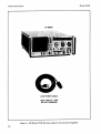
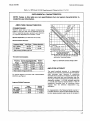
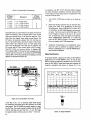
Figure 1-1. HP Model 8569B Spectrum Analyzer with Accessories Supplied
1-0
General Information
ModeI8569B
SECTION I
GENERAL INFORMATION
1-1. INTRODUCTION
1-9.
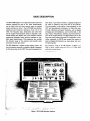
1-2. This Operation and Service manual contains
information required to install, operate, test, adjust,
and service the Hewlett-Packard Model 8569B Spectrum Analyzer. Figure 1-1 shows the instrument and
accessories supplied. This section covers instrument
identification, description, options, accessories,
specifications, and other basic information.
1-10. This manual is divided into eight sections as
follows:
1-3.
DESCRIPTION
1-4. The HP Model 8569B Spectrum Analyzer provides a visual display of RF and microwave signals in
the frequency domain. Input signal amplitude is plotted on the CRT as a function of frequency.
1-5. The HP Model 8569B is designed for simplicity of operation. Most measurements can be made
using only three controls, once the normal settings
(marked in green) have been preset. The HP Model
8569B has absolute amplitude and frequency calibration from 10 MHz to 22 GHz. The frequency span,
bandwidth, and video filter are all coupled with
automatic sweep time to maintain a calibrated display and to simplify operation of the analyzer.
1-6. Internal preselection eliminates most spurious
images and multiple responses to simplify signal
identification. The preselector also extends dynamic
range of the analyzer and provides some protection
for the input mixer.
1-7. The frequency range of the HP Model 8569B
is 10 MHz to 22 GHz in direct coaxial input and 12.4
to 115GHz when used with external mixers.
1-8. The HP Model 8569B has a digital display
with the spectral information contained in either of
two independent traces. Major control settings are
annotated on the CRT above the graticule area. Signal processing controls for the digital display include
trace normalization, a maximum hold function, digital averaging, and trace storage. A hard-copy record
of the display may be obtained through direct instrument control of listen-only plotters. The HP Model
8569B has an HP-IB capability that allows controller
interrogation of display information or controller
entry of messages and trace data.
MANUAL ORGANIZATION
SECTION I, GENERAL INFORMATION, contains the instrument description and specifications,
explains accessories and options, and lists recommended test equipment.
SECTION II, INSTALLATION AND OPERATION VERIFICATION, contains information concerning initial mechanical inspection, preparation for
use, operating environment, packaging and shipping,
and operation verification.
SECTION III, OPERATION, contains detailed
operating instructions for operation of the instrument.
SECTION IV, PERFORMANCE TESTS, contains
the necessary tests to verify that the electrical operation of the instrument is in accordance with published specifications.
SECTION V, ADJUSTMENTS, contains the necessary adjustment procedures to properly adjust the
instrument after repair.
SECTION VI, REPLACEABLE PARTS, contains
the information necessary to order parts and/or
assemblies for the instrument.
SECTION VII, MANUAL BACKDATING
CHANGES, contains backdating information to
make this manual compatible with earlier equipment
configurations.
SECTION VIII, SERVICE, contains schematic diagrams, block diagrams, component location illustrations, circuit descriptions, and troubleshooting information to aid in repair of the instrument.
1-11.
SPECIFICATIONS
1-12. Instrument specifications are listed in Table
1-1. These specifications are the performance standards or limits against which the instrument is tested.
1-1
Model 8569B
General Information
Table 1-2 lists supplemental characteristics. Supplemental characteristics are not specifications but are
typical characteristics included as additional information for the user.
NOTE
To ensure that the HP Model 8569B
meets the specifications listed in
Table 1·1, performance tests (Section
IV) should be performed every six
months.
1·13.
SAFETYCONSIDERATIONS
1-14:. ~efore operating this instrument, you should
~arrulianze yourself with the safety markings on the
Instrument and safety instructions in this manual
This instrument has been manufactured and tested
according to international safety standards. However, to ensure safe operation of the instrument and
personal safety of the user and service personnel, the
cautions and warnings in this manual must be followed. Refer to individual sections of this manual for
?etailed safety notation concerning the use of the
Instrument as described in those individual sections.
1·15.
Safety Symbols
Instruction manual symbol: the apparatus will
be marked with this symbol when It is neeessary for the user to refer to the instruction
manual in order to protect the apparatus
against damage.
Indicates dangerous voltages.
Earth terminal
I
WARNING
I
The WARNING sign denotes a haz·
ard. It calls attention to a proeedure, practice, or the like, which, If
not correctly performed or adhered
to, could result In Injury or loss of
life. Do not proceed beyond a
WARNING sign until the Indicated
conditions are fully understood
and met.
The CAUTION sign denotes a haz·
ard. It calls attention to an operat·
ing procedure, practice, or the like,
which, If not correctly peformed or
adhered to, could result in damage
to or destruction of part or all of
the equipment. Do not proceed
beyond a CAUTION sign until the
Indicated conditions are fully
understood and met.
1-2
1·16.
Service
1-17. Although this instrument has been manufactured in accordance with international safety standards, this manual contains information, cautions
and warnings which must be followed to insure safe
operation and to keep the instrument safe. Service
should be performed only by qualified service personnel, and the following warnings should be
observed:
I
WARNINGS'
Any maintenance or repair of the
opened instrument under voltage
should be avoided as much as posslble, and when inevitable, should be
carried out only by a skilled person
who is aware of the hazard involved.
Capacitors inside the instrument may
still be charged even if the instrument
has been disconnected from its
source of supply.
Make sure that only fuses with the
required rated current and of the
specified type (normal blow, time
delay, etc.) are used for replacement.
The use of repaired fuses and the
short·circuiting of fuseholders must
be avoided.
When it is likely that the protection
has been impaired, the instrument
must be made inoperative and be
secured against any unintended operation.
If this instrument is to be energized
via an auto-transformer (for voltage
reduction) make sure the common terminal is connected to the earthed
pole of the power source.
BEFORE SWITCHING ON THE
INSTRUMENT, the protective earth
terminals of the instrument must be
connected to the protective conductor of the mains power cord. The
mains plug shall only be inserted in a
socket outlet provided with a protective earth contact. The protective
action must not be negated by the
use of an extension cord (power cord)
General Information
Model 8569B
without a protective conductor
(grounding). Grounding one conductor of a two conductor outlet is not
sufficient protection.
Any interruption of the protective
(grounding) conductor (inside or outside the instrument) or disconnecting
the protective earth terminal is likely
to make this instrument dangerous.
BEFORE SWITCHING ON THIS
INSTRUMENT, make sure instrument's ac input is set to the voltage of
the ac power source (see Figure 2·1).
BEFORE SWITCHING ON THIS
INSTRUMENT, make sure the ac line
fuse is of the required current rating
and type (normal-blew, time delay,
etc.).
1·18. INSTRUMENTS COVERED BY MANUAL
1·21. Manual Changes Supplement
1-22. An instrument manufactured after the printing of this manual may have a serial number prefix
that is not listed on the title page. This unlisted serial
number prefix indicates the instrument is different
from those described in this manual. The manual for
this newer instrument is accompanied by a yellow
Manual Changes supplement. This supplement contains "change information" that explains how to
adapt the manual to the newer instrument.
1-23. In addition to change information, the supplement may contain information for correcting
errors in the manual. To keep this manual as current
and accurate as possible, Hewlett-Packard recommends that you periodically request the latest Manual Changes supplement. The supplement carries a
manual identification block that includes the model
number, print date of the manual, and manual part
number. Complimentary copies of the supplement
are available from Hewlett-Packard. Addresses of
Hewlett-Packard offices are located at the back of
this manual.
1·24. Manual Backdating Changes
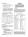
1·19. Serial Numbers
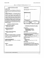
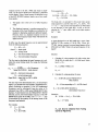
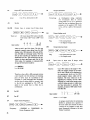
1-20. Attached to the rear of each section of your
instrument is a serial number plate (Figure 1-2). The
serial number is in two parts. The first four digits
and letter are the serial number prefix; the last five
digits are the suffix. The prefix is the same for all
identical instruments; it changes only when a change
is made to the instrument. The suffix, however, is
assigned sequentially and is different for each instrument. The contents of this manual apply to instruments with the serial number prefix(es) listed under
SERIAL NUMBERS on the title page.
1-25. Instruments manufactured before the printing of this manual have been assigned serial number
prefixes other than those for which this manual was
written directly. Manual backdating information is
provided in Section VII to adapt this manual to any
such earlier assigned serial number prefix.
1-26. This information should not be confused
with information contained in the yellow Manual
Changes supplement, which is intended to adapt this
manual to instruments manufactured after the printing of this manual.
1·27. OPTIONS
-
SERIAL NUMBER
PREFIX
....
,
SUFFIX
.....
sER,2J03A01726
OPT
f7h,i . HE WLE r t, f->ACKARD
l
'\./1"
J
".~
".l '
It..
,A
Figure 1-2. Typical Serial Number Plate
1·28. Option 001
1-29. Option 001 provides an internally connected,
l00-MHz comb generator that is switched in by a
front-panel push button.
1·30. Option 002
1-31. Option 002 deletes the two most narrow RESOLUTION BW settings, .3 kHz and .1 kHz, provided on the standard instrument.
1-3
Mode18569B
General Information
1·32.
Option 400
1-33. Option 400 permits operation on 50, 60, and
400 Hz mains. All specifications are identical to
those of the standard HP Model 8569B except for
operating temperature range and power requirements (see Table 1-1).
1·34. Option 908, Rack Flange Kit
1-35. Option 908, HP Part Number 5061-0078,
includes flanges and hardware required to mount the
HP Model 8569Bin an equipment rack with horizontal spacing of 482.6 mm (19 in.), See Figure 2-2 for
installation procedure.
1·36. Option 910, Additional Operation and
Service Manual
1-37. One additional Operation and Service Manual is provided for each Option 910 ordered.
To obtain Option 910 after shipment of the instrument, specify the manual part number printed on the
title page of the manual.
1·38. Option 913, Rack Flange/Front Handle
Kit
1-39. Option 913, HP Part Number 5061-<>084,
combines a Front Handle Kit with Option 908, Rack
Flange Kit. See Figure 2-2 for installation procedure.
1·42. EQUIPMENT AVAILABLE
1·43. Service Accessories
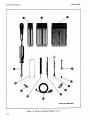
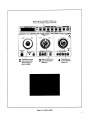
1-44. A Service Accessories Package is available
for convenience in aligning and troubleshooting the
spectrum analyzer. The Service Accessories Package
is shown in Figure 1-3. The package may be obtained
from Hewlett-Packard by ordering HP Part Number
08569-60035.
1·45. Measurement Accessories
1·46. HP Model 11517A External Mixer. This
mixer extends the frequency range of the HP Model
8569B to 40 GHz. Transition sections (HP Models
11518, 11519A, and 11520A) are available to adapt
the HP Model 11517A External Mixer to standard
waveguide sizes.
1·47. HP Model 197B, Option 006 Oscllloscope Camera. This camera can be used with the
Model 8569B to make a permanent record of measurements.
1·48. Transit Case. A polyethylene transit case,
HP Part Number 1540-0654, is available for protection of the HP 8569BSpectrum Analyzer.
1·49. RECOMMENDED TEST EQUIPMENT
1-40.
ACCESSORIES SUPPLIED
1-41. Figure 1-1 shows the HP Model 8569B Spectrum Analyzer and line power cord. One 5Q-ohm termination (HP 1810-01180, connected to the frontpanelIST LO OUTPUT port, is also supplied.
1-4
1-50. Equipment required for operation verification, performance tests, adjustments, and troubleshooting of the HP Model 8569B is listed in Table 13. Other equipment may be substituted if it meets or
exceeds the critical specifications listed in the table.
Model 8569B
General Information
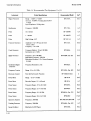
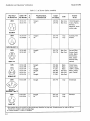
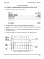
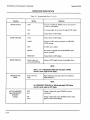
Table 1-1. HP Model 8569B Specifications (1 of 3)
SPECI FICATIONS
FREQUENCY SPECIFICATIONS
FREQUENCY RANGE
Internal mixing 0.01 to 22 GHz
Covered in six ranges selectable by Frequency Band
push buttons (in GHz): .01 to 1.8; 1.7 to 4.1; 3.8 to 8.5;
5.8 to 12.9;8.5 to 18; 10.5to 22.
External mixing 12.4to 115 GHz
Covered in four ranges selectable by Frequency Band
push buttons (in GHz): 12.4-26.5 (6+ harmonic mode);
21-44 (10+ harmonic mode); 33-71 (16+ harmonic
mode); and 53-115 (26+ harmonic mode).
FREQUENCY ACCURACY
Tuning Accuracy
The overall tuning accuracy of the digital frequency
readout in any span mode:
.01 to 115 GHz
± (5 MHz or 0.2% of center frequency, whichever is
greater, + 20% of frequency span per division)
CRT digital readout resolution (included in tuning
accuracy)
Internal mixing, 100 kHz; external mixing, 1 MHz
Center Frequency
The center frequency represented by the CRT is indicated by the digital frequency displays on the front
panel and the CRT.
Zero Span
Analyzer becomes a manually tuned receiver (for the
time domain display of signal modulation) set to the
frequency indicated by the digital frequency
displays.
SPECTRAL RESOLUTION AND STABILITY
Resolution Bandwidths
Resolution (3 dB) bandwidths from.1 kHz to 3 MHz in
1,3 sequence. Bandwidth may be varied independently or coupled to Frequency SpanlDiv control. Optimum coupling (convenient ratio of Frequency
SpanlDiv to Resolution Bandwidth) is indicated by
alignment of markers (~~) on both controls.
Uncoupled, the controls for Frequency SpanlDiv and
Resolution Bandwidth may be independently set so
any resolution bandwidth (3 MHz to .1 kHz) may be
used with any span width (F and 500 MHz to 1
kHz/Div). Analyzer is calibrated if UNCAL is not
displayed.
Resolution Bandwidth accuracy
Individual resolution bandwidth 3 dB points:
< ±15%.
Selectivity: (60 dB/3 dB bandwidth ratio) < 15:1 for bandwidths 3 kHz to 3 MHz; < 11:1 for bandwidths.1 kHz
to 1 kHz.
FREQUENCY SPANS
(on a 10 division CRT horizontal axis)
1.7t022GHz
Multiband span of spectrum from 1.7 to 22 GHz in one
sweep. The frequency (position) corresponding to the
tuning marker is set by the Tuning control and indicated by the digital frequency displays on the front
panel and the CRT.
Full Band
Displays spectrum of entire Frequency Band
selected. Tuning marker displayed in Full Band mode
(becomes center frequency when Per Divison mode is
selected). Marker frequency is given on the digital
displays.
Stability
Total residual FM
Stabilized: < 100 Hz POp in 0.1 sec, .01- 4.1 GHz
Unstabilized: < 10 kHz pop in 0.1 sec, .01- 4.1 GHz
(Fundamental mixing)
Stabilization range: First LO automatically stabilized
(unless auto stabilizer is OFF) for frequency spans
100 kHz/Div or less.
Noise sidebands: At least 75 dB down, greater than
30 kHz from center of CW signal when set to a 1
kHz Resolution Bandwidth and a 10 Hz (.01) Video
Filter (fundamental mixing).
AMPLITUDE SPECIFICATIONS
Per Division
Eighteen calibrated spans from 1 kHzl Div to 500
MHz/Div in a 1, 2, 5,10 sequence. In "F" position the
entire Frequency Band selected is spanned.
AMPLITUDE RANGE - Internal mixer
Span width accuracy
The frequency error for any two points on the display
for spans from 500 MHz to 20 kHz/Div (unstabllized) is
less than ±5% of the indicated separation; for
stabilized spans 100 kHz/Div and less, the error is
less than ± 15%.
Measurement range:
Damage levels:
Total RF power: + 30 dBm (1 watt)
de or ac « < 500 source impedance):
OV with 0 dB input attenuation (1 amp); ± 7V
with <!:10 dB input attenuation (0.14 amp)
1-5
General Information
Mode18569B
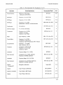
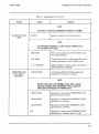
Table 1-1 HP Model 8569B Specifications (2 of 3)
Peak pulse power:
+ 50 dBm «10!"sec. pulse width, 0.01 % duty
cycle), ;?: 20 dB attentuation
Gain compression:
< 1 dB for - 7 dBm input level with 0 dB attenuation.
Average Noise Level:
Sensitivity (minimum discernible signal) is given by the
signal level which is equal to the average noise level, causing approximately a 3-dB peak above the noise. Maximum
average noise level with 1 kHz Resolution Bandwidth (0 dB
attenuation and 0.003 (3 Hz) video filter) is given in the
table below. Sensitivity in the external mixing bands (harmonic modes 6 +,10 +,16 + and 26 +) assumes an external mixer conversion loss of 30 dB.
Frequency
Band (GHz)
First IF
In MHz
Harmonic
Mode
Avg. Noise Level
(dBm)
.01·1.8
2050
1-
-113
1.7-4.1
321.4
1-
-110
3.8-8.5
321.4
2-
-107
5.8·12.9
321.4
3-
-100
8.5-18
321.4
4+
-95
-90
10.5-22
321.4
5+
12.4-26.5
321.4
6+
-104
21-44
321.4
10+
-104
33-71
321.4
16+
-104
53-115
321.4
26+
-104
Reference Level
Reference Level range: +60 dBm' to -112 dBm in 10
dB steps and continuous 0 to -12 dB calibrated
vernier.
Reference Level accuracy:
With Sweep TimelDivision control in Auto setting, the
optimum sweep rate is selected automatically for any
combination of Frequency Span/Div, Resolution
Bandwidth and Video Filter settings. Thus, the Auto
Sweep setting insures a calibrated amplitude display
within the following limits:
Input Attenuator (at preselector input, 70 dB range
in 10 dB steps)
Step size variation:
o to 60 dB, 0.01-18 GHz: < ± 1.0 dB
o to 40 dB, 0.01·22 GHz: < ± 1.5 dB
Maximum cumulative error:
o to 60 dB, 0.01-18 GHz: < ±2.4 dB
oto 40 dB, 0.01-22 GHz: < ± 2.5 dB
Frequency Response (with 0 or 10 dB of Input
Attenuation)
Frequency response includes input attenuator,
preselector and mixer frequency response plus
mixing mode gain variation (band to band) and
assumes preselector peaking.
Frequency Band (GHz)
.01-1.8
1.7-4.1
3.8-8.5
5.8-12.9
8.5·18
10.5-22
Frequency Response
(± dB MAX.)
1.2
1.5
2.5
2.5
3.0
4.5
Switching between bandwidths: 3 MHz to 300 kHz,
< ± 0.5 dB; 3 MHz to 0.1 kHz, < ± 1.0 dB.
Calibrated display range
Log expanded from reference level down:
70 dB with 10 dBlDiv scale factor
40 dB with 5 dB/Div scale factor
16 dB with 2 dBlDiv scale factor
8 dB with 1 dB/Div scale factor
Linear: Full scale from 0.56 !"V (-112 dBm across 50
ohms to 224 volts (+60 dBm)' in 10 dB steps and continuous 0 to -12 dB vernier. Full scale signals in
linear translate to approximately full scale signals in
the log modes.
Display accuracy
Log: < ± 0.1 dB/dB but not more than ± 1.5 dB over
70 dB display range.
Linear: < ± 3% of reference level.
Calibrator output
-10dBm ±0.3dB
100 MHz :to 10 kHz
Residual responses (no signal present at input):
With 0 dB input attenuation and fundamental mixing
(0.01 to 4.1 GHz): < - 90 dBm.
Reference Level variation (Input Attenuator at 0
dB)
10 dB steps, + 20°C to + 30°C:
-10to -70dBm: < ±0.5dB·
-10to -100dBm: < ±1.0dB
-10to -70dBm: < ±1.0dB,0°Cto +55°C
Signal Identifier:
Provided over entire frequency range and in all Frequency Span / Div. settings. Correct response is a 2
MHz shift to left and approximately a 6 dB lower
amplitude. (Reads incorrectly for 100 MHz CAL OUTPUT Signal.)
Ilnput level not to exceed +30 dBm damage level.
1-6
Vernier (0 to -12 dB) continuous: Maximum error
< ±0.5 dB, when read from Reference Level Fine
control.
Model 8569B
General Information
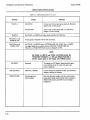
Tab/e 1-1. HP Mode/8569B Specifications (] of])
SWEEP SPECIFICATIONS
SWEEP TIME
Auto: Sweep time is automatically controlled by Frequency SpanlDiv, Resolution Bandwidth and Video Filter
controls to maintain an absolute amplitude calibrated
display.
Calibrated Sweep times: 21 internal sweep times from
21'secIDiv to 10 seclDiv in 1,2,5 sequence. Sweep time
accuracy ± 10% except for 2, 5, and 10 sec/Div, which
are ±20%. Swept frequency modes use sweep times 2
mseclDiv through 10 seclDiv. When operated as a fixed
tuned receiver (Zero Span) the full range of sweep·times
(2 I'sec to 10 seclDiv) may be used to display modulation
waveforms. Sweep times that are too fast or too slow for
the Resolution Bandwidth, Frequency Span/ Div, and
Video Filter settings (producing an uncalibrated display)
are indicated by an UNCAL warning on the CRT. Sweep
times :5 2 mseclDiv (:5 5 mseclDiv when in Max Hold, Digital Averaging, or INP-B....A Normalization) produce a
mixed mode display with analog traces and CRT control
readouts on the CRT.
GENERAL SPECIFICATIONS
LO OUTPUT (2.00 to 4.46 GHz):
+7 dBm minimum, 0 to 35°C;
DIMENSIONS
458 mm wide: 188 mm high, 565 mm deep (18 in. x
73/8 in. x 22 1/4 in.)
~.JI!1..D...n.
..
-rt
TOP
JJ U "
_
l.---468mm (18 in.I-----1-r!----565 mm 122.25in.,~
:l ~ .". M~
""
It
STANDARD OPTIONS AVAILABLE
+ 5 dBm minimum, 35 to 55°C.
TEMPERATURE RANGE:
Operating O°C to 55°C
Storage - 40° C to + 75°C.
HUMIDITY RANGE (Operating):
< 95% R.H. O°C to +40°C.
EMI:
Conducted and radiated interference is in compliance
with MID-STD 461A Methods CE03 and RE02, CISPR
publication 11 (1975) and Messempfaenger- Postverfuegung 526/527/79 (Kennzeichnung Mit F- Nummer/Funkschutzzeichen).
POWER REQUIREMENTS
48-Q6 Hz; 100,120,220 or 240 volts (-10% to + 5%); 220 VA
maximum. Fan cooled.
OPTION 001
Intemal100 MHz Comb Generator
Frequency Range: 0.01 to 22 GHz
Frequency Accuracy: :5 ± 0.007%
OPTION 002
Deletes .3 kHz and .1 kHz resolution BW settings.
All specifications Identical to standard HP 8569B except:
Spectral Resolution and Stability
Resolution Bandwidths: Resolution (3 dB) bandwidths from 1 kHz to 3 MHz in a 1, 3 sequence.
Selectivity: (60 dB/3 dB bandwidth ratio) < 15:1 for bandwidths 1 kHz to 3 MHz.
Stability
Total Residual FM
Stabilized: <200 Hz pop in 0,1 sec..01-4.1 GHz.
OPTION 400
Permits operation on 48-440 Hz mains.
WEIGHT:
Net:
29.1 kg (64 Ibs.)
Shipping: 40.9 kg (90 Ibs.)
All specifications Identical to standard HP 8569B except:
Power requirements: 48 to 440 Hz; 100, 120, 220 or 240
volts (-10% to + 5%); 220 VA maximum. Fan cooled.
'Input level not to exceed + 137 dBI'V damage level.
1-7
General Information
Model 8569B
Table 1-2. HP Model 8569B Supplemental Characteristics (1 of 4)
SUPPLEMENTAL CHARACTERISTICS
NOTE: Values in this table are not specifications but are typical characteristics lncluded for user information.
With Temperature Changes:
Stabilized
< 10 kHz/·C
Unstabilized <200 kHZ/·C
Auto stabilizer may be disabled in narrow spans
« 100 kHz/Div) by depressing front panel
pushbutton switch to "OFF" position.
FREQUENCY CHARACTERISTICS
FREQUENCY SPANS
1.7t022 GHz
When this mode is selected the analyzer displays the
entire spectrum from 1.7 to 22 GHz. A 3 MHz Resolu·
tion Bandwidth, 9 kHz Video Filter, and 100 msec/div
Sweep Time are automatically selected.
Full Band
When selected by panel pushbutton, analyzer
displays spectrum of Frequency Band chosen. This
automatically selects a 3 MHz Resolution bandwidth
and a 9 kHz Video Filter. Sweep Time/Div varies from
approximately 10 msec to 100 msec/div depending on
which Frequency Band is chosen. Tuning marker frequency (position) indicates where analyzer tuning will
be centered If a Per Division span mode is chosen.
Per Division
In "F" position (full band), the entire range of the Frequency Band selected is spanned, thus allowing the
use of Resolution Bandwidth and Video Filter settings other than those chosen when the Full Band
pushbutton is depressed. Center frequency of the
analyzer's display is set by the tuning control and indicated by the LED readouts. The Frequency CAL
control to the right of the display window on the front
panel is used to set the LED readout to agree with the
actual center frequency of the CRT display (normally
set using the 100 MHz CAL OUTPUT as a 0.100 GHz
frequency reference).
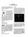
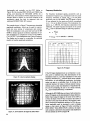
VIDEO FILTER
Video Filter bandwidths typically ± 20% of nominal
value.
Post detection low-pass filter used to average
displayed noise for a smooth trace. Nominal settings
are given as decimal fractions of the Resolution
Bandwidth: OFF, .3, .1, .03, .01, and .003. A 1 Hz
NOISE AVG (noise averaging) setting is provided for
noise level measurement.
,:~
~
1\
~
~
\
~
~
"
40
1\
1\
\
\
\
~
~~
60
'1\
~
'I
'I
~
1\
,~
i\
80
100 Hz
1 kHz
1\,
~
~
~
\
\
%
50
70
Out-of-range blanking
The out-of-range portion of the CRT trace is automatically blanked whenever the analyzer is swept
beyond a band edge.
\
\
\
\
'0
\
10kHz
100 kHz
'\
1 MHz
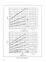
SIGNAL SEPARATION
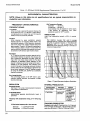
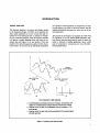
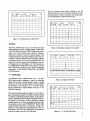
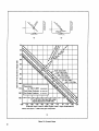
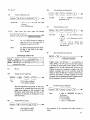
Figure 1. Typical Spectrum Analyzer Resolution
RESOLUTION
INTERNALPRESELECTOR
Bandwidth Ranges
See Figure 1 for curves of typical analyzer resolution
using different IF bandwidths.
IF Bandwidth shape:
Approximately gaussian (synchronously tuned, 4pole filter)
Freauency Ranae
DeacrlDtlon
ReJection
0.01 to 1.8 GHz
Low-pass filter
1.7to22GHz
Tracking YIG
tuned filter
>50 dB above
2.05GHz
> 70 dB greater
than 642.8 MHz
from center of
pass band 1.7
to 18GHz.
>60 dB from 18
to 22 GHz
Frequency drift (fundamental mixing, .01-4.1 GHz) long
term
At fixed center frequency after 1 hour warm·up:
Stabilized
Unstabilized
1-8
< ±3.0 kHz/10 minutes
< ±25 kHz/10 minutes
TRACKING PRESELECTOR
Preselector skirt roll-off: Characteristics of a three-pole
filter (nominally 18 dB/octave), 3 dB bandwidth typically
varies from 25 MHz (at 1.7 GHz)to 70 MHz (at 22 GHz).
10MHl
Model 8569B
General Information
Table 1-2 HP Model 8569B Supplemental Characteristics (2 of 4)
SUPPLEMENTAL CHARACTERISTICS
NOTE: Values in this table are not specifications but are typical characteristics tneluded for user information.
~
AMPLITUDE CHARACTERISTICS
I
20
30 -
DYNAMIC RANGE
~
t
60
Spurious responses: (Input attenuator set to 0 dB)
~
70
~
80
90
Second harmonic distortion
!
-
I"
~"
Icc.f:_",,-,
09 ~:"/..,~o
... ' i!:i'~I:>'--L----i_-+----i_-f
Input Power
Relative Distortion
0.01 ·1.8 GHz
-40dBm
< -70dB
1.7-22GHz
+30dBm
< -130dB"
0g:,,,q,(:j
<Q' '" :-.,....-+---;--+---1
~I:"
~(
-:
1~1·i
~(I€../+.-+---;--+---;--+---1
t---+-+--.. .~~-/,~-::·i\..
..
f·.....
i:: Sensl:~v~~HZBW)
;
120
"May be below average noise level
130
~O
j,-10.5-22.0 GHz
~~m·---~;~'Q.
8+::...,..;~':":~+·~.-=:':":~~::..j.z--!---1
...
Frequency Range
~ -1:"1 /,,~'"
I
-
l.:__
50
1"/
::-...."
I",
40
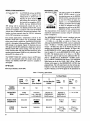
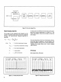
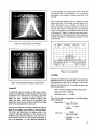
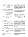
Maximum power ratio of two signals simultaneously
present at the input that may be measured within the
limits of specified accuracy, sensitivity and distortion
(i.e., spurious responses): 0.01 to 22 GHz > 70 dB.
if./
::' J; :"'-----~__l--+-~
2nd Order Products - - 3rd Order produ~ •• _ _•
_ '_ ~
3.8'~.5 6Hz
-.I"
~~i'~W~:I'~
I
1.7~.1 GHz
0.01-1.8 GHz
,~~
I
-
I -; - - : -
_..I_..l{to
L··_··-l.··_'··_··_·l-··T-··~~·
tI ~~
22 GHz (2nd end 3rd order)
.........
I
ISignel Separetion;ol00 MHz
-70 -60 -so ~ -30 -20 -10
O' +10 +20 +30
Effective Input Level in dBm (Signel Level-Input Attenuetion)
Third order Intermodulation
Frequency
Range
0.01·22GHz
For Two Input Signals With
Total Power
Signal 5ep.
-30dBm
~SOkHz
Relative
< -70dB
1.7·12.9GHz
-10dBm
~70MHz
< -130dB"
1.7·22GHz
-10 dBm
~ 100 MHz
< -130dB"
"May be below average noise level
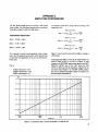
For typical harmonic and third order intermodulation
distortion, see Figure 2.
Image and MUltiple Responses:
Imlge
Figure 2. Optimum Dynamic Range Chart
Distortion
Frequency
(oul of bind)
Multiple
(In-bind)
0.01-1.8 GHz
1.7-18GHz
18-22GHz
< -SOdB
<-70dB
< -60dB
non-existent
< -70dB
< -60dB
AMPLITUDE ACCURACY
The overall amplitude accuracy of a measurement
depends on an analyzer's performance and the measurement technique used. Applying IF substitution
eliminates errors caused by the display, bandwidth gain
variation, scale factor and input attenuator step size.
Only IF gain variation (reference level change with input
attenuation constant: < ± 0.5 dB), calibrator amplitude
« ± 0.3 dB), and frequency response remain. In brief, IF
substitution minimizes error by minimizing control
changes from the reference measurement (e.g.,
calibration).
For measurements in the Frequency Bands covering 1.7
to 22 GHz that don't require the best possible accuracy,
the front panel preselector peak may be left centered in
1-9
General Information
Model 8569B
Table 1-2. HP Model 8569B Supplemental Characteristics (3 of 4)
SUPPLEMENTAL CHARACTERISTICS
NOTE: Values in this table are not specifications but are typical characteristics lneluded for user information.
its "green" setting. Best amplitude accuracy is obtained
by peaking the preselector at the frequency of interest.
Reference Level Variation (For any change of scale taetor): < ± 1 dB.
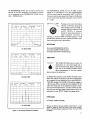
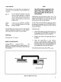
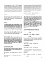
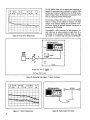
FREQUENCY RESPONSE AND AVERAGE
NOISE LEVEL
For typical frequency response and average noise level
versus input frequency, see Figure 3.
1--+--+--t---t--+--+--t--+-+-----1f--i
~YPICAl~REaUE~CYRESP~NSE EX~URSIONILIMITS
I
I
I
-10
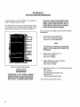
Input Protection (For input signals from .01 to 22 GHz)
0.01 to 1.8 GHz Frequency Band: Internal diode
limiter.
1.7 to 22 GHz Frequency Bands: Saturation of YIG
filter (preselector) occurs at total input signal power
levels below input mixer damage.
EXTERNAL MIXING IF INPUT
SMA female connector is a port for 321.4 MHz IF input
signals and bias current. Internal gain adjustments have a
range of 10 to 45 dB.
SWEEP CHARACTERISTICS
•
SWEEP SOURCE
1--+--+--t---t--+--+--t--+-+-----1f--i
-!.,...---
-..--f---+--+--+--+--+---+--+--+----;--i
I
-00
1--+-+-+---+-+-+--1--+-.j-.....If--i
, kHI I SPECIFIE!? I
F-120
-
-----
I,...-f--+-~_-oof-____
I
I--H
10
12
'4
16
18
20
-10
Manual: Sweep determined by front panel control: continuously settable across CRT in either direction.
External: Sweep determined by 0 to + 10V external
signal applied to External Sweep input on rear panel.
Blanking is controlled by signal at Blanking Input.
Operation in Digital Storage Display mode with External
sweep requires a Retrace signal input to rear panel
Retrace Input connector.
Internal: Sweep
generator.
generated
from
internal
sweep
SWEEP TRIGGER
Free Run: Sweep triggered repetitively by internal
source.
22
FReQUENCY' GHI I
Figure 3. Typical Frequency Response and
A verageNoise Level Versus Input Frequency
SIGNAL INPUT CHARACTERISTICS
Line: Sweep triggered by power line frequency.
Video: Sweep internally triggered by detected waveform
of input signal (signal amplitude of 0.5 division peak-topeak required on CRT display).
INPUT 500 0.01 TO 22 GHz
Input connector: Precision type N female
Input Impedance
Input attenuator at 0 dB: 50 ohms nominal
SWR: < 1.5 0.01 to 1.8 GHz
<2.0 1.7 to 22 GHz (at analyzertuned
frequency)
Input attenuator at 10 dB or more: 50 ohms nominal
SWR: < 1.3 0.01 to 1.8 GHz
<2.0 1.7to22GHz
LO Emission (2.00 to 4.46 GHz):
< - 60 dBm 0.01 to 1.8 GHz
< -SOdBm 1.7t022GHz
1-10
Trigger Level: Sets the level of the sweep trigger signal,
whether it is the displayed trace (Video mode) or an external trigger input (Ext mode).
External Trigger: Sweep triggering determined by signal
input (between + 1 and + 10 volts) to rear panel BNC
connector.
Single: Sweep triggered or
Start/Reset pushbutton.
reset
by
front
panel
Start/Reset: Triggers sweep in Single sweep mode. Can
also reset any internal sweep to left edge of display.
Model 8569B
General Information
Table 1-2 HP Model 8569B Supplemental Characteristics (4 of 4)
SUPPLEMENTAL CHARACTERISTICS
NOTE: Values in this table are not specifications but are typical characteristics included for user information.
INPUT/OUTPUT CHARACTERISTICS
Plotter Interface
Log: < 0.1 dB/dB, max error < 1 dB
Linear: < 0.1 division
x, V, and
Z Axis Outputs: These outputs are compatible
with and may be used to drive all current HP XV
recorders (using positive pencoils or TIL penlift input)
and CRT monitors.
Horizontal Sweep Output (X axis): A voltage proportional
to the horizontal sweep of the CRT trace which ranges
from - 5V for the left graticule edge to + 5V for the right
graticule edge. Output impedance is 5 kohms.
Vertical Output (V axis): Detected video output proportional to vertical deflection of the CRT trace. Output increases 100 mV/div from 0 to 800 mV (from a 50 ohm
source) for a full 8-division deflection. Output impedance is 50 ohms.
Blank (Penlift or Z axis) Output: A blanking output, 15V
from 10 kohms, Which occurs during CRT retrace or
when sweeping beyond band edges. Otherwise output is
low at OV with a 10 ohm output impedance for a normal
or unblanked trace (pen down).
Blanking Input: Permits remote Z axis control of CRT
with TIL levels; normal < 0.5V or open circuit, blank
> 2V. Input impedance is 10 kohms. Note that in Digital
Storage mode, Blanking input does not directly blank
the CRT; instead it sets blank bits in the trace memory
so that the appropriate parts of the trace are blanked
during the CRT refresh cycle.
Caution: maximum input is ±40V.
External Sweep Input: When the front panel Sweep
Source switch is set to the EXT mode, a 0 to 10V ramp
will sweep the analyzer through the frequency range
determined by front panel Tuning and Frequency Span/Div
controls. Input impedance is 100 kohms.
Caution: maximum input is
±
40V
External Trigger Input: With the Sweep Trigger in EXT
mode, a signal will trigger a sweep on the signal's
positive slope between + 1 and + 10 volts according to
the setting of the Trigger Level control. 100 kohms input
impedance, de coupled.
Caution: maximum input
±
40V.
21.4 MHz IF Output: A 50 ohm, 21.4 MHz output linearly
related to the RF input to the analyzer. Bandwidth controlled by the analyzer's Resolution Bandwidth setting;
amplitude controlled by the Input Attenuator, IF gain vernier and first 6 IF Reference Level step gain positions
(-10 through - 60 dBm level with 0 dB input attenuation). Output is approximately - 10 dBm from 50 ohms
for full scale signals on the CRT.
First LO Output: Connector is SMA Female, 50 ohms.
Terminate in a 50 ohm load When not in use.
Frequency: 2.00 to 4.46 GHz
Power Level: typically + 8 dBm minimum
Stability (Typical residual FM):
Stabilized: 30 Hz pop
Unstabilized: 2 kHz pop
External Mixing Bias: -5 mA to +5 mA Onto 500 D.s) output from the EXT MIX ING IF INPUT port. Maximum short
circuit current limits: ±9 mA, maximum open circuit voltage
limits: ±3 volts.
Aux B: Used during factory calibration.
CATHODE RAY TUBE
Type: Post deflection accelerator, approximately 11.5 kV
accelerating potential, aluminized P31 phosphor,
electrostatic focus and deflection.
Graticule: Internal 8 x 10 division. 1 division vertically is
1 centimeter, 1 division horizontally is 1.2.centimeters.
There are 5 subdivisions per each major division.
Caution: maximum input ± 40V.
Retrace Input: Required for operation in Digital Storage
Display mode if External Sweep is used. Normal level
<O.5V, blank (retrace) level >2V. Input impedance is 10
kohms.
Annotation: Major control settings are annotated on
CRT.
Viewing Area: Approximately 9.6 centimeters vertically
by 11 centimeters horizontally (3.8 inches by 4.7 inches).
1-11
Model 8569B
General Information
HP PART NO. 08565-60100
Figure 1-3. Service Accessories Package (1 of 2)
1-12
Model 8569B
General Information
!
C
D
HP Part
Number
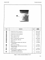
Extender board, 6 pin (12 conductors)
8
08505-60109
Extender board, 15 pin (30 conductors)
7
08505-60041
Extender board, 22 pin (44 conductors)
8
08565-60107
Wrench, 15/64 inch open end
8
871O'{)946
Adapter, SMA male to male
3
1250-1158
Wrench, 5/16 inch slotted box end/open end
9
08555-20097
Adapter, BNC female to SMA male
6
1250-1200
Alignment tool
7
871O.{)630
Item
0
••
••
••
•
0
CD
•
••
•
Jillillllil
Description
Test cable, subminiature (SMC) female to BNC male
(36 inches long)
11592-60001
Alignment tool, non-metallic
4
871O.{)033
Adapter, BNC female to SMC female (used to measure
second LO output)
3
08565-60087
Connector extractor
6
8710.{)580
Tuning tool (consists of modified 5/16 inch nut driver
with modified No. 10 Allen driver)
6
08555-60107
Extender board, 40 pin (80 conductors)
9
08569-60013
Figure 1-3. Service Accessories Package (2 of 2)
1-13
Model 8569B
General Information
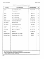
Table 1-3. Recommended Test Equipment (1 of 3)
Instrument
Critical Specifications
Recommended Model
Use*
Digital Voltmeter
Range: -IOOOV to +1OOOV
Accuracy: ±O.004% of reading pluse 0.001 %
of range
Input Impedance: 10 Meg ohms
HP 3455A
P,A,T
Oscilloscope
Frequency: 100 MHz
HP1741A
A,T
Probe
10: 1 Divider
HP 10004D
A,T
Probe
1: 1 Divider
HP 10007D
A,T
Probe
High Voltage, 4 kV
HP 34111A
A,T
Function Generator
Amplitude: 0 to +1OVpop sine wave
with de offset
Frequency: 1 to 5 kHz
HP 3312A
P,A,T
Comb Generator
Frequency Markers: 10 and 100 MHz
Increments up to 5 GHz
HP 8406A
P,A
Signal Generator
Frequency: 50 to 500 MHz
Modulation Frequency: 100 kHz
Modulation Deviation: 1% of lowest frequency
in range
HP 8640B, Opt. 001
P,A,T
Synthesized Signal
Generator
Frequency Resolution: 2 Hz
HP8662A
P
Frequency Counter
Range: .01 to 24.5 GHz
HP 5342A, Opt. 005
P,A,T
Electronic Counter
Time Interval Counter Function
HP 5300A/5302A
A
Power Meter
Range: -20 to +10 dBm
HP435B
P,A,T
Power Meter
Recorder Output: 1V = full scale
HP432A
A,T
Power Sensor
Frequency Range: .05 to 26.5 GHz
HP 8485A
P,A,T
Power Sensor
Frequency Range: 12.4-18.0 GHz
HPP486C
P,A,T
Power Sensor
Frequency Range: .01-18 GHz
HP 8481 A, Opt. C03
P,A,T
Power Sensor
Frequency Range: 18.0-26.5 GHz
HPK486C
P,A,T
Spectrum Analyzer
Frequency: 300 MHz
HP 140T/8552B/8554B
A,T
Tracking Generator
Frequency: 300 MHz
HP 8444A, Opt. 059
A,T
Sweep Oscillator
Mainframe for RF Plug-in
HP 8350A
P,A,T
1-14
General Information
Model 8569B
Table 1-3. Recommended Test Equipment (2 of 3)
Critical Specifications
Instrument
Recommended Model
Use*
Sweep Oscillator
Mainframe for RF Plug-in
(Alternate for HP 8350A)
HP 8620C
P,A,T
RF Plug-in
Frequency: .01 to 26.5 GHz
HP 83595A
A,T
RF Plug-in
Frequency: .01 to 2.4 GHz
HP 86222A
P,A
RF Plug-in
Frequency: 2 to 22 GHz
Residual FM: <30 kHz in 10kHz Bandwidth
HP 86290A, Opt. H08
P,A,T
Synchronizer
No Substitute
HP 8709A, Opt. H10
A
DC Power Supply
4 to 6 volts de (Floating)
HP 62l4A
A
Termination
Frequency: de to 18 GHz
Impedance: 50 ohms
Connector: Type N Male
HP 909A, Opt. 012
P
Mixer
Input Frequency: 23 GHz
HP 11517 A, Opt. E03
P
Power Splitter
Frequency: 2 to 18 GHz
Attenuation: 6 dB each arm
Connectors: Type N Female Input APC-7 Outputs
HP 11667 A, Opt. 002
P,A
Crystal Detector
Frequency: .1 to 22 GHz
Input Connector: APC-3.5
HP 33330C
P,A,T
Attenuator
Attenuation: 10 dB ±0.5 dB
Frequency: .01 to 18 GHz
Connectors: Type N
HP 8491B, Opt. 010
P,A
Attenuator
Frequency Range: 12.4-18 GHz
HPP382C
A
Step Attenuator
Attenuation: 0 to 12 dB in 1-dB steps
Frequency: 100 MHz, Calibrated
HP 355C, Opt. H80
P,A
Attenuator
Frequency Range: 18.0-26.5 GHz
HP K382C
A
Step Attenuator
Attenuation: 0 to 120 dB in lO-dB steps
Frequency: 100 MHz, Calibrated
HP 355D, Opt. H80
P,A
Adapter
(2 required)**
Waveguide to SMA Jack
Narda 4608
P,A
Adapter
Type N Female to BNC Male
HP 1250-0077
P
Adapter (2 required)
Type N Male to BNC Female
HP 1250-0780
P,T
Adapter
Type N Plug to SMA Jack
HP 1250-1250
P,T
1-15
General Information
Model 8569B
Table 1-3. Recommended Test Equipment (3 of 3)
Instrument
Critical Specifications
Recommended Model
Use*
HP 08565-60087
A,T
Adapter**
BNC Female to SMC Female
Adapter
K-Band to R-Band; for use with
HP 11517 A Mixer
HP l1519A
P
Adapter
APC-7 to Type N Female
HP 11524A
P,A
Adapter
APe-7 to Type N Male
HP 11525A
P,A
Adapter
APe-7 to SMA Female
HP 11534A
P,A
Adapter
Type N Female to SMA Female
HP 86290-60005
P,T
Adapter (2 required)
Type N Male to SMA Female
HP 1250-1404
P,T
Cable Assembly
SMA Plug both ends
HP 8120-1578
P,T
Cable Assembly
Type N Connector both ends
HP 11500A
P,T
BNC Short
Impedance: 50 ohms
HP 1250-0774
A
BNC Tee
Connectors: BNC Jack and Plug
HP 1250-0781
A
Test Cable**
SMA Female to BNC Male
HP 11592-60001
P
Diplexer
No Substitute
Directional Coupler
Frequency Range: 12.4-18.0 GHz
HPP752C
P,A
Directional Coupler
Frequency Range: 18.0-26.5 GHz
HPK752C
P,A
*p = Performance Test; A = Adjustment; T = Troubleshooting
**These parts are included in Service Accessories Package; HP Part Number 08565-60100
***Only one required if HP 86290A. Opt. H08 used
1-16
HP 5086-7721
Installation and Operation Verification
Model 8569B
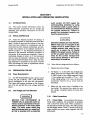
SECTION II
INSTALLATION AND OPERATION VERIFICATION
2·1. INTRODUCTION
earth contact. DO NOT negate the
earth-grounding protection by using
an extension cable, a power cable, or
an autotransformer without a protective ground conductor. Failure to
ground the instrument properly can
result in personal injury.
2-2. This section includes information about the
initial inspection, preparation for use, storage and
shipment, and operation verification for the HP
Model 8569B.
2-3.
INITIAL INSPECTION
2-4. Inspect the shipping container for damage. If
the shipping container or cushioning material is damaged, it should be kept until the contents of the shipment have been checked for completeness and the
instrument has been checked mechanically and electrically. The contents of the shipment should be as
shown in Figure 1-1. The electrical performance is
checked by the operation verification procedure in
this section. If the contents are incomplete, if there is
mechanical damage or defect, or if the instrument
does not pass the operation verification test, notify
the nearest Hewlett-Packard office. Keep the shipping materials for inspection by the carrier. The HP
office will arrange for repair or replacement without
waiting for a claim settlement.
BEFORETURNING ON THIS INSTRUMENT, make sure it is adapted to the
voltage of the ac power source. The
voltage selector card must be correctly set to adapt the HP Model
8569B to the power source. Failure to
set the ac power input of the instrument for the correct voltage level
could cause damage to the instrument when it is turned on.
2-9. Select the line voltage and fuse as follows:
1. Measure the ac line voltage.
2·5.
PREPARATION FOR USE
2-6.
Power Requirements
2-7. The HP Model 8569B requires a power source
of 100, 120,220, or 240 Vac + 5OJo -10%,48-66 Hz.
Power consumption is less than 220 volt-amperes.
The Option 400 permits operation on line frequencies of 50, 60, and 400 Hz at the voltages specified
above.
2-8.
2.
See Figure 2-1. At the power line module (rear
panel), select the line voltage (l00v, 120V, 220V,
or 240V) closest to the voltage measured in step
1. Line voltage must be within + 5% or - 10%
of the voltage setting. If it is not, use an autotransformer between the ac source and the
instrument.
3.
Make sure the correct fuse is installed in the
fuse holder. The required fuse rating for each
line voltage is indicated below the power line
module.
Line Voltage and Fuse Selection
I
WARNING
I
BEFORE THIS INSTRUMENT IS
TURNED ON, its protective earth terminals must be connected to the protective conductor of the main power
cable. The main power cable plug
shall be inserted only in a socket outlet that is provided with a protective
2-10.
Cable Connections
2-11. Power Cable. In accordance with international safety standards, this instrument is equipped
with a three-wire power cable. When connected to
the appropriate power line outlet, this cable grounds
the instrument cabinet. Table 2-1 shows the styles of
plugs available on power cables supplied with HP
instruments.
2-1
Model 8569B
Installation and Operation Verification
Table 2-1. A C Power Cables Available
Plug Tvpe,"
AC Source End
Cable,* HP
Part Number
C
D
250V
8120-1351
8120-1703
0
6
8120-3169
8120~696
~
L
Plug Description,
Instrument End
Country
of Use
Length
cm (inches)
Color
Straight
90°
229 (90)
229 (90)
Mint Gray
Mint Gray
0
4
Straight
90°
201 (79)
221 (87)
Gray
Gray
Australia, New
Zealand
8120-1689
8120·1692
7
2
Straight
90°
201 (79)
201 (79)
Mint Gray
Mint Gray
East and West
Europe, Saudi
Arabia, Egypt,
South Africa,
India, (unpolarized in many
nations)
8120-1348
8120-1398
8120-1754
8120-1378
8120·1521
8120-1676
5
5
7
1
6
2
Straight
90°
Straight
Straight
90°
Straight
293 (80)
203 (80)
91 (36)
203 (80)
203 (80)
91 (36)
Black
Black
Black
Jade Gray
Jade Gray
Jade Gray
United States,
Canada,Japan
(IOOYor 200Y),
Mexico, Philippines, Taiwan
8120-2104
3
Straight
201 (79)
Gray
Switzerland
8120·1957
8120-2956
2
3
Straight
90°
201 (79)
201 (79)
Gray
Gray
Denmark
N
United Kingdom,
Cyprus, Nigeria,
Rhodesia,
Singapore, South
Africa, India
BS1363A
250V
@
NZSS198/ASC112
250V
@
N
L
CEE7·Y11
125V
~
NEMA5·15P
250V
@
N E L
SEV1011
1959·24507 Type12
220V
~
N
L
DHCK 107
*Part number shown for source end plug is industry identifier for plug only. Number shown for cable is HP Part
Number for complete cable including plugs.
E = Earth Ground; L = Line; N = Neutral
2-2
Installation and Operation Verification
Model 8569B
I
WARNING
I
If this instrument is to be energized
through an autotransformer, make
sure the common terminal of the
autotransformer is connected to the
protective earth contact of the power
source outlet socket.
Any interruption of the protective
ground, inside or outside the instrument, can make it a shock hazard.
2-12.
Mating Connectors
2-13. All mating connectors on the HP Model
8569B Spectrum Analyzer have standard HewlettPackard part numbers and are readily available.
2-14.
Operating Environment
2·15. Temperature. The instrument may be
operated in tempertures from O°C to + 55°C.
2·16. Humidity. The instrument may be operated in environments with humidity from 5070 to 95%
at O°C to 40°C. However, the instrument should also
be protected from temperature extremes that cause
internal condensation.
2·17. Altitude. The instrument may be operated
at altitudes up to 4572 meters (15,000 feet).
2·18.
Bench Operation
2-19. The cabinet of the instrument has plastic feet
and foldaway tilt stands for convenience in bench
operation. The tilt stands raise the front of the
instrument for easier viewing of the control panel.
The plastic feet are shaped to make full width modular instruments self-aligningwhen stacked.
2·20.
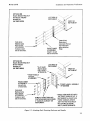
Rack Mounting (Options 908 and 913)
2-21. Instruments with Option 908 are shipped with
a Rack Flange Kit, which supplies necessary hardware, with installation instructions, for mounting the
instrument on a rack whose spacing is 482.6 mm (19
inches). Installation instructions are also given in Figure 2-2. See Table 2-2 for HP part numbers.
2-22. Instruments with Option 913 are shipped with
a Rack Flange/Front Handle Kit, which supplies
necessary hardware, with installation instructions,
for the addition of front handles and mounting the
instrument on a rack whose spacing is 482.6 mm (19
inches). Installation instructions are also given in Figure 2-2. See Table 2-2 for HP part numbers.
2·23.
Front Handles
2-24. Instruments are shipped with a Front Handle
Kit, which supplies necesary hardware, with installation instructions, for mounting front handles on the
instrument. See Figure 2-2 for installation instructions.
Table 2-2. Rack-Mounting Kits for HP 8569B
C
D
HP Part
Number
Quantity
Rack Flange
8
502008863
2
Machine Screw, Pan Head,
8·32 x 0.375 inch
7
2510.0193
8
Handle Assembly
0
5060·9900
2
Rack Flange
2
502008875
2
Machine Screw, Pan Head,
8·32 x 0.625 inch
8
2510.0194
8
Description
OPTION 908
OPTION 913
2-3
Installation and Operation Verification
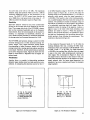
Model 8569B
RECEPTACLE FOR PRIMARY POWER CORD
PC SELECTOR BOARD SHOWN POSITIONED
FOR 115/120 VAC POWER LINE.
SELECTION OF OPERATING VOLTAGE
OPERATING VOLTAGE APPEARS IN MODULE WINOOW.
SLIDE OPEN POWER MODULE COVER DOOR
AND PUSH FUSE-PULL LEVER TO LEFT TO
REMOVE FUSE.
2. PULL OUT VOLTAGE-5ELECTOR PC BOARD.
POSITION PC BOARD SO THAT VOLTAGE
NEAREST ACTUAL LINE VOLTAGE LEVEL
WILL APPEAR IN MODULE WINDOW. PUSH
BOARD BACK INTO ITSSLOT.
3. PUSH FUSE-PULL LEVER INTO ITSNORMAL
RIGHT-HAND POSITION.
4. CHECK FUSE TO MAKE SURE IT IS OF CORRECT RATING AND TYPE FOR INPUT AC
LINE VOLTAGE. FUSE RATINGS FOR DIFFERENT LINE VOLTAGES ARE INDICATED
BELOW POWER MODULE.
5. INSERT CORRECT FUSE IN FUSEHOLDER.
1.
Figure 2-1. Line Voltage Selection with Power Module PC Board
2-4
Model 8569B
Installation and Operation Verification
OPTION 908
RACK MOUNTING KIT
WITHOUT FRONT
HANDLES
(HP 5061-0078)
///
~
/
/ / -:
~ - : -: e
PAN HEAD
~/
Machine Screw
TRIM STRIP
8-32 x 0.375" _--..-,~
HP 2510-0193
RACK FLANGE
HP 5020-8863
4 places on each
side of instrument.
Attach 1 on each
side of instrument.
OPTION 913
RACK MOUNTING KIT
WITH FRONT
HANDLES
(HP 5061-0084)
LEFTSIDEDF
INSTRUMENT
*FLAT-HEAD
Machine Screw
*FRONT HANDLE
Trim Strip
HP 5020-8897
RACK FLANGE
HP 5020-8875 ---~~
~ .>.
<; T~", ~~
Y
/-<><-1-y)
" <,
8-32 x 0.375"
HP 2510-0195
(on each side
of instrument).
(Each side of
instrument) Remove
from instrument
before attaching
flange.
/
.~
-~'"
FRONT OF
INSTRUMENT
---/~
/%f'/~Friil~ == .-: '
-: %?
"".... /' -III_
l!J« /' -
/~/ ~
.XJ
*FRONT HANDLE ASSEMBLY
HP 5060-9900
*THESE ITEMS SUPPLIED WITH
THE FRONT HANDLES KIT. IF
REMOVE TRIM STRIPS AND
INSTRUMENT ALREADY HAS
FLAT-HEAD MACHINE SCREWS
FRONT HANDLES, ORDER
IF HANDLES ALREADY ON
JUST THE PAN HEAD MACHINSTRUMENT.
INE SCREWS (2510-0194)
AND FLANGES (5020-8875).
Figure 2-2. Attaching Rack Mounting Hardware and Handles
2-5
Installation and Operation Verification
Item
0
••
•
e•
Qty
8
C
D
Model 8569B
HP Part No.
Description
7
9220-2733
FOAM PADS-TOP CORNER; BOTTOM CORNER
4
9211-2622
CARTON-INNER
4
3
4040-1738
BARS-SHIPPING, PLASTIC
8
9
2510-0103
SCREW-FOR ATTACHING SHIPPING BARS
(REMOVE HANDLES FOR SHIPMENT)
5
9211-2623
CARTON-OUTER
9
9220-2735
SIDE PADS, CORRUGATED CARDBOARD
2
9222-0069
BAG, PLASTIC
2
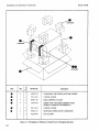
Figure 2-3. Packaging for Shipment Using Factory Packaging Materials
2-6
Installation and Operation Verification
Model 8569B
2-25.
STORAGE AND SHIPMENT
2·26.
Environment
2-27. The instrument may be stored or shipped in
environments within the following limits:
Temperature
Humidity
Altitude
- 40°C to + 75°C
5% to 95010 at O°C to 40°C
Up to 15,240 meters
(50,000 feet)
service required, return address, model number,
and full serial number. A supply of these tags is
provided at the end of this section.
2.
Use a strong shipping container. A double-wall
carton made of 350-pound test material is adequate.
3.
Use enough shock-absorbing material (3-inch to
4-inch layer) around all sides of the instrument
to provide firm cushion and prevent movement
inside the container. Protect the control panel
with cardboard.
4.
Seal the shipping container securely.
5.
Mark the shipping container FRAGILE to
assure careful handling.
The .instrument should also be protected from temperature extremes that cause internal condensation.
2·28.
Packaging
2-29. Original Packaging. Containers and
materials identical to those used in factory packaging
are available through Hewlett-Packard offices. Figure 2-3 illustrates the proper method of packaging
the instrument for shipment using factory packaging
materials. If the instrument is being returned to
Hewlett-Packard for servicing, attach a tag indicating the type of service required, return address,
model number, and full serial number. A supply of
these tags is provided at the end of this section. Also
mark the container FRAGILE to assure careful handling. In any correspondence, refer to the instrument
by model number and full serial number.
2·30. Other Packaging. The following general
instructions should be used for repackaging with
commercially available materials:
1.
Wrap the instrument in heavy paper or plastic.
If shipping to a Hewlett-Packard office or service center, attach a tag indicating the type of
2·31.
OPERATION VERIFICATION
2-32. The Operation Verification is designed to test
only the most critical specifications and operating
features of the instrument. It requires much less time
and equipment than the complete performance tests
listed in Section IV and is recommended for verification of overall instrument operation, either as part of
incoming inspection or after repair. The Operation
Verification consists of the following tests:
•
Operational Check
•
Tuning Accuracy
•
Frequency Span Width with Resolution Bandwidth Accuracy
•
Amplitude Accuracy
2-7
Installation and Operation Verification
Model 8569B
OPERATION VERIFICATION
NOTE
Allow at least 30 minutes warrn-up time.
EQUIPMENT:
Frequency Counter. . . . . . . . . . . . . . . . . . . . . . . . . . . . . . . . . . . . . . . . . . . . . . . . . . . . . .. HP 5340A
HP 8406A
Comb Generator
HP 435B
Power Meter
HP 8481A
Power Sensor
HP 355D
Step Attenuator (10 dB/Step)
NOTE
If substitution is necessary for any of the above listed equipment, the alternate models must meet or exceed the critical specifications listed in Table
1-3.
2·33.
OPERATIONAL CHECK
PROCEDURE:
1.
Perform front-panel adjustment procedure provided on pull-out card.
2.
Connect comb generator (100 MHz comb) to HP 8569B INPUT 500 connector. Set all normal (green)
settings, except set TRACE A and TRACE B to STORE BLANK. Set FREQUENCY SPAN/DIV to 1
MHz and TUNING to 0.100 GHz. Verifyindication noted in Table 2-3for each setting shown.
NOTE
In checking some functions, first press CLEAR/RESET to clear digital trace
from CRT display.
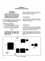
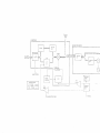
2·34. TUNING ACCURACY
SPECIFICATION:
Overall tuning accuracy of the digital frequency readout in any span mode:
Internal Mixing:
± (5 MHz or 0.2070 of center frequency, whichever is greater, plus 20% of frequency span per division)
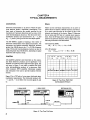
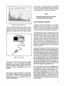
DESCRIPTION:
The tuning accuracy of the HP 8569B is verified by means of a comb generator at the first two FREQUENCY
BAND GHz settings. The CAL OUTPUT frequency is measured, and the HP 8569B is calibrated at 100 MHz.
The comb generator is then connected to the INPUT 500 connector of the HP 8569B, and the tuning accuracy
is checked.
2-8
Model 8569B
Installation and Operation Verification
OPERATION VERIFICATION
2·34.
TUNING ACCURACY (Cont'd)
PROCEDURE:
1. Connect frequency counter to spectrum analyzer CAL OUTPUT as shown in Figure 2-4. Set all normal
(green) settings, and other controls as follows:
TRACE A . . . . . . . . . . . . . . . . . . . . . . . . . . . . . . . . . . . . . . . . . . . . . . . . . . . . . . . . . . . . . . .. WRITE
TRACE B
, . . . . . . . .. STORE BLANK
FREQUENCY BAND GHz . . . . . . . . . . . . . . . . . . . . . . . . . . . . . . . . . . . . . . . . . . . . . . . .. .01 - 1.8
TUNING
O.IOOGHz
10 dB
INPUT AITEN
REF LEVEL dBm
- 10
REFERENCE LEVEL FINE . . . . . . . . . . . . . . . . . . . . . . . . . . . . . . . . . . . . . . . . . . . . . . . . . . . . .. 0
FREQUENCY SPAN/DIV . . . . . . . . . . . . . . . . . . . . . . . . . . . . . . . . . . . . . . . . . . . . . . . . . .. 1 MHz
RESOLUTION BW
30 kHz
MIXING MODE
INT
POWER
METER
SPECTRUM ANALYZER
FREOUENCYCOUNTER
INPUT
10 Hz- 250 MHz
I
,
:
,
STEP
I
AITENUATOR :
l-A-~
I
_ _P~OWER SENSOR __
1
,
.'.
"
COMB
GENERATOR
••••
• •
000
OUTPUT
Figure 2-4. Operation Verification Test Setup
2-9
Installation and Operation Verification
Model8S69B
OPERATION VERIFICATION
2·34.
TUNING ACCURACY (Cont'd)
2. Measure spectrum analyzer CAL OUTPUT frequency using frequency counter. Reading should be 100
MHz ± 0.01 MHz.
3.
Calibration of FREQUENCY GHz display is initially adjusted at 100 MHz. Connect CAL OUTPUT to
INPUT son and tune instrument to center signal on CRT display. FREQUENCY GHz readout should be
0.100. If necessary, adjust FREQ CAL screwdriver adjustment for 0.100 on FREQUENCY GHz display.
Check that CTR annotation on CRT reads 100.0 MHz.
4.
Verifycalibration of FREQUENCY GHz display in other frequency bands as follows:
2·35.
a.
Tune instrument for an indication of 1.800 GHz on FREQUENCY GHz digital readout.
b.
Connect comb generator to spectrum analyzer INPUT 500 and tune instrument to center 1.8 GHz
comb tooth on CRT display. FREQUENCY GHz readout must be 1.800 ±0.005 GHz.
c.
Select 1.7 - 4.1 FREQUENCY BAND GHz and set TUNING control for an indication of 3.000 GHz
on FREQUENCY GHz readout.
d.
Center 3.0 GHz comb tooth on CRT display. FREQUENCY GHz readout must be 3.000 ±0.006
GHz.
e.
Set TUNING control for an indication of 4.000 GHz on FREQUENCY GHz readout.
f.
Center 4.0 GHz comb tooth on CRT display. FREQUENCY GHz readout must be 4.000 ±0.008
GHz.
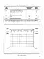
FREQUENCY SPAN WIDTH AND RESOLUTION BANDWIDTH ACCURACY
SPECIFICATION:
Span width accuracy: The frequency error for any two points on the display for spans from 500 MHz to 20
kHz/Div (unstabilized) is less than ± 5070 of the indicated separation; for stabilized spans 100 kHz/Div and less,
the error is less than ± 15%.
Resolution bandwidth accuracy: Individual resolution bandwidth 3 dB points:
< ± 15%.
DESCRIPTION:
A comb generator is used to check the span width and the CAL OUTPUT signal is used to check resolution
bandwidth accuracy at different positions of the FREQUENCY SPAN/DIV and RESOLUTION BW controls.
By verifying the calibration of these controls, proper operation of the sweep circuits is also verified.
PROCEDURE:
1. Connect comb generator to instrument INPUT 500.
2-10
Installation and Operation Verification
Model 8569B
OPERATION VERIFICATION
2·35.
2.
FREQUENCY SPAN WIDTH AND RESOLUTION BANDWIDTH ACCURACY (Cant'd)
Set all normal (green) settings, and other controls as follows:
Spectrum Analyzer:
TRACE A . . . . . . . . . . . . . . . . . . . . . . . . . . . . . . . . . . . . . . . . . . . . . . . . . . . . . . . . . . . . . . .. WRITE
TRACE B . . . . . . . . . . . . . . . . . . . . . . . . . . . . . . . . . . . . . . . . . . . . . . ..
STORE BLANK
FREQUENCY BAND GHz . . . . . . . . . . . . . . . . . . . . . . . . . . . . . . . . . . . . . . . . . . . . . . . .. .01 - 1.8
FREQUENCY SPAN/DIV . . . . . . . . . . . . . . . . . . . . . . . . . . . . . . . . . . . . . . . . . . . . . . . .. 100 MHz
RESOLUTION BW
1 MHz (coupled)
INPUT ATTEN
10 dB
REF LEVEL dBm
0
TUNING
0.500 GHz
Comb Generator:
Comb frequency
Output amplitude
100 MHz
Optimum
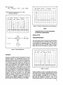
3.
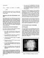
Tune spectrum analyzer to position one comb tooth at graticule reference line (far left).
4.
Note position of ninth spectral line (comb tooth). It must be on eighth graticule line ± 0.4 division. (See
Figure 2-5.)
5.
Set FREQUENCY SPAN/DIV to 10 MHz (with RESOLUTION BW coupled) and comb generator to 10
MHz. Repeat steps 3 and 4.
6.
Set FREQUENCY SPAN/DIV to 1 MHz and comb generator to 1 MHz. Repeat steps 3 and 4.
FIRST
GRATICUlE
LINE
CTR
REF
604.0 MHz
SPAN 100 MHz/
RES BW 1 MHz
o dBm
10 dB/
ATTEN 10 dB
SWP AUTO
-- ...............
GRATICUl E
E __
REFERENC
LINE
COMB
SIGNALS
---
FIRST
SPECTRAL
LINE
-
~
I
- V-
r---..
VF OFF
EIGHTH
GRATICUlE
LINE
---...
---
NINTH
SPECTRAL
LINE
'V'Y
Figure 2-5. Span Width Accuracy Measurement
2-11
Model 8569B
Installation and Operation Verification
OPERATION VERIFICATION
2-35.
FREQUENCY SPAN WIDTH AND RESOLUTION BANDWIDTH ACCURACY (Cont'd)
NOTE
The wider FREQUENCY SPAN/DIV settings are checked using a comb generator, The narrow FREQUENCY SPAN/DIV settings are checked by observing RESOLUTION BW accuracy as follows:
7.
Set FREQUENCY SPAN/DIV to .2 MHz, RESOLUTION BW to 1 MHz, and AMPLITUDE SCALE to
I dB.
8.
Connect spectrum analyzer CAL OUTPUT to INPUT 500 and tune spectrum analyzer to 0.100 GHz.
Center signal on display and use REFERENCE LEVEL controls to position peak of signal to REFERENCE LEVEL line.
9.
Note width of signal three divisions below REFERENCE LEVEL line. Specification: 5 divisions ±0.75
division. Verification of the I MHz RESOLUTION BW setting verifies proper operation of the LC bandwidth filters.
10.
Set FREQUENCY SPAN/DIV to 10 kHz and RESOLUTION BW to 30 kHz.
11.
Repeat step 8 and note width of signal three divisions below REFERENCE LEVEL line. Specification: 3
divisions ± 0.45 division. Verification of the 30 kHz RESOLUTION BW setting verifies proper operation
of the crystal bandwidth filters.
2-36_
AMPLITUDE ACCURACY
SPECIFICATIONS:
Calibrator Output: - 10 dBm ± 0.3 dB
Reference Level variation (Input Attenuator at 0 dB):
10 dB steps, + 20°C to + 30°C:
Oto -60dBm: <±0.5 dB
oto - 90 dBm: < ± 1.0 dB
Vernier (0 to - 12 dB) continuous:
Maximum error < ± 0.5 dB, when read from REFERENCE LEVEL FINE control.
Input Attenuator (at preselector input, 70 dB range in 10 dB steps):
Step size variation (for steps from 0 to 60 dB):
Oto 60 dB, 0.01-18 GHz: <± 1.0dB
oto 40 dB, 0.01 - 22 GHz: < ± 1.5 dB
Maximum cumulative error:
oto 60 dB, 0.01-18 GHz: < ±2.4 dB
oto 40 dB, 0.01- 22 GHz: <±2.5 dB
2-12
Model 8569B
Installation and Operation Verification
OPERATION VERIFICATION
2·36.
AMPLITUDE ACCURACY (Cont'd)
PROCEDURE:
1. Set all normal (green) settings, and other controls as follows:
FREQUENCY SPAN/DIV . . . . . . . . . . . . . . . . . . . . . . . . . . . . . . . . . . . . . . . . . . . . . . . . . .. 1 MHz
RESOLUTION BW
30 kHz (coupled)
FREQUENCY BAND GHz . . . . . . . . . . . . . . . . . . . . . . . . . . . . . . . . . . . . . . . . . . . . . . . .. .01 - 1.8
TUNING
O.looGHz
INPUT ATTEN
10 dB
REF LEVEL dBm
- 10
REFERENCE LEVEL FINE
. . . . . . . . . . . . . . . . . . . . . . . . . . . . . . . . . . . . . . . .. 0
AMPLITUDE SCALE. . . . . . . . . . . . . . . . . . . . . . . . . . . . . . . . . . . . . . . . . . . . . .. 1 dB LOG/DIV
2.
Measure CAL OUTPUT signal level with a power meter. Specification: - 10 dBm ± 0.3 dB.
3.
Connect 100 MHz CAL OUTPUT signal through 355D step attenuator (set to 0 dB) to INPUT 500 and
tune spectrum analyzer to center signal on CRT display. Position peak of signal at REFERENCE LEVEL
line with front-panel REF LEVEL CAL screwdriver adjustment.
4.
To verify correct operation of the REFERENCE LEVEL FINE (Vernier) control, set 355D step attenuator
to 10 dB. Set REFERENCE LEVEL FINE to - 9. The peak of the signal on the CRT display should be
one division below the REFERENCE LEVEL ± 0.5 division « ± 0.5 dB). Return 355D step attenuator to
OdB.
5.
Set INPUT ATTEN to 70 dB, REF LEVEL dBm to 0, REFERENCE LEVEL FINE to - 8, RESOLUTION BW to 3 kHz, FREQUENCY SPANIDIV to 1 kHz, and VIDEO FILTER to .03. Center signal on
CRT display with TUNING control.
6.
Adjust REF LEVEL CAL to position signal peak two divisions below REFERENCE LEVEL line.
7.
Step instrument INPUT ATTEN from 70 to 0 dB while stepping 355D step attenuator from 0 to 70 dB
(maintain a total attenuation of 70 dB). For each 10 dB step, the signal amplitude should not change more
than ± 1 dB from the previous step. The total amplitude variation (difference betwen maximum and
minimum signal levelsover entire 70 dB range) should not exceed 2.4 dB.
8.
Adjust REF LEVEL CAL to position signal peak two divisions below REFERENCE LEVEL line.
9.
Step instrument REF LEVEL dBm from -70 to -10 while stepping 355D step attenuator from 70 dB to
10 dB (maintain signal level approximately two divisions below REFERENCE LEVEL line ± 0.5 division
(±0.5dB).
2-13
Installation and Operation Verification
Model 8569B
OPERATION VERIFICATION
Table 2-3. Operational Check (1 of 3)
Function
SWEEP SOURCE
SWEEP TRIGGER
SWEEP TIME/DIV
Setting
Indication
MAN
Rotation of MANUAL SWEEP control varies position
of trace on CRT display.
EXT
No sweep. Bright dot on lower left edge of CRT display.
INT
Sweep visible on CRT display.
LINE
Sweep visible on CRT display.
VIDEO
Presence of CRT sweep is dependent on TRIGGER
LEVEL setting.
EXT
No CRT trace is visible.
SINGLE
One sweep is triggered when START/RESET pushbutton is pressed.
FREE RUN
Sweep visible on CRT display.
Slowly rotate control counterclockwise.
Sweep on CRT display becomes increasingly slower.
NOTE
Select 1.7-4.1 FREQUENCY BAND GHz and adjust TUNING
control to center signal on CRT display.
PRESELECTOR
PEAK
Rotate over full
range.
Signal amplitude varies. (Set control for maximum
signal amplitude.)
NOTE
Set FREQUENCY SPAN/DIV to 100kHz and adjust FINE tuning
control to center signal on CRT display.
AUTO STABILIZER
(Blue FREQUENCY
SPAN/DIY
settings)
2-14
OFF
(in)
Tuning of signal with coarse TUNING control is
continuous.
ON
(out)
Tuning of signal with coarse TUNING control causes
signal to jump off CRT display.
Installation and Operation Verification
Model 8569B
Table 2-3. Operational Check (2 of 3)
Function
Setting
Indication
NOTE
Set TRACE A to WRITE and FREQUENCY SPAN/DIV to 100MHz.
FREQUENCY SPAN
MODE
Signals are displayed at one-division intervals.
PERDIV
NOTE
Set FREQUENCY SPAN/DIV to .2 MHz and adjust TUNING control
to center signal on CRT display.
AMPLITUDE SCALE
(Center signal on
CRT display.)
ZERO SPAN
CRT trace is a straight line and FINE TUNING control
affects signal amplitude.
FULL BAND
Twenty-five comb teeth are visible and baseline marker
position is determined by coarse TUNING control.
1.7-22 GHz SPAN
Baseline is displayed from left to right in five steps (see
Section III). Return to PER DIV.
10 dB (LOG/DIV)
10 dB change in REF LEVEL dBm changes signal
amplitude by one division ±O.l division.
NOTE
Set REF LEVEL dBm and REFERENCE LEVEL FINE to position
signal peak 0.5 division below REFERENCE LEVEL graticule line.
Center signal on CRT display with TUNING control.
5 dB (LOG/DIV)
Signal peak one division below REFERENCE LEVEL
graticule line (±O.25 division).
2 dB (LOG/DIV)
Signal peak 2.5 divisions below REFERENCE LEVEL
graticule line (±O.6 division).
1 dB (LOG/DIV)
Signal peak 5 divisions below REFERENCE LEVEL
graticule line (±1.2 divisions).
LIN
Signal peak 3.5 divisions below REFERENCE LEVEL
graticule line (±l.O division). Return to 10 dB.
2-15
Mode18569B
Installation and Operation Verification
OPERATION VERIFICATION
Table 2-3. Operational Check (3 of 3)
Setting
Function
TRACE A
TRACEB
TRACES A and B
STORE BLANK
TRACES A and B
STORE VIEW
Indication
MAX HOLD
Increase and then decrease signal amplitude. Maximum
signal is held on CRT display.
STORE VIEW
Trace is held on CRT display and is not affected by
changes in control settings.
Set TRACE A to WRITE and repeat checks described for TRACE A.
Analog signal is displayed without CRT annotation.
Set TRACE A to WRITE, then to STORE BLANK. With TRACE B set to WRITE,
vary signal amplitude or position, then set TRACE B to STORE VIEW. Set
TRACE A to STORE VIEW. Both traces are displayed on CRT.
NOTE
Set TRACE A to WRITE and TRACE Bto STORE BLANK. Set
FREQUENCY SPAN/DIV to 1 MHz and RESOLUTION BW to
30 kHz. Center signal on CRT display with TUNING control.
SIG IDENT
2-16
Depressed
Two signals on CRT display. Signal identifier signal
is two divisions to left of comb tooth and is also
lower in amplitude.
CRT Annotation
TRACE A to WRITE
Control settings are displayed on CRT, and annotation
changes as settings are changed.
VIDEO FILTER
Step through each
switch position
Each step decreases baseline noise level and decreases
sweep speed. Sweep speed increases when switching to
NOISE AVG position, and CRT trace is virtually a
straight line.
Model 8569B
Installation and Operation Verification
Table 2-4. Operation Verification Test Record
Hewlett-Packard Company
Mode18569B
Tested by
Serial Number
Date
Results
Para.
No.
Test Description
2-34
-0.4 div
-0.4 div
-0.4 div
+0.4 div
+0.4 div
+0.4 div
4.25 div
2.55 div
5.75 div
3.45 div
-10.3 dBm
-9.7 dBm
0.5 div
1.5 div
Input Attenuator Accuracy
7. Error Between Adjacent Settings
8. Error Over 60 dB Range
2-36.
1.805
3.006
4.008
Vernier (0-12 dB)
4. Vernier Accuracy
2-36.
1.795
2.994
3.992
Calibrator Output Power
2. CAL OUTPUT Signal
2-36.
ioo.or
Resolution Bandwidth Accuracy
9. 1 MHz RESOLUTION BW
11. 30 kHz RESOLUTION BW
2-36.
99.99
Span Width Accuracy
4. 100 MHz FREQUENCY SPAN/DIV
5. 10 MHz FREQUENCY SPAN/DIV
6. 1 MHz FREQUENCY SPAN/DIY
2-35.
Max.
Tuning Accuracy
4b. 1.8 GHz
4d. 3.0 GHz
4f. 4.0 GHz
2-35.
Actual
Calibrator Output Accuracy
2. 100 MHz
2-34.
Min.
±1.0 div
±2.4 div
Reference Level Variation
9. Reference Level Variation in
LOG,O to -60 dB
±0.5 div
2-17/2-18
Operation
Mode18569B
SECTION III
OPERATION
3·1.
INTRODUCTION
3-2. This section is published separately as "8569B
Spectrum Analyzer Operation," HP Part Number
08569-90034. It describes typical applications of signal analysis and provides detailed instructions for
both local (front-panel) and remote (HP-IB) operation.
3-3. A table of contents is provided at the beginning of this section.
3·4.
ROUTINE MAINTENANCE
3·5.
Fuses
3-6. The HP 8569B has nine fuses, eight of which
are internal. Only the ac line fuse, located at the back
of the instrument, may be replaced by the operator.
The ac line cord should be disconnected from the
power source, then the other end disconnected from
the instrument. With the power cord removed, access
the fuse compartment by sliding open the clear plastic cover on the power module. Remove the fuse by
pulling the lever inside the fuse compartment.
Replace the blown fuse with a fuse of the correct
rating and type for the ac line voltage selected. Fuse
ratings for different voltages are indicated below the
power module. Access to the other eight fuses
requires removal of the covers of the instrument. The
internal fuses should be replaced by a qualified service technician.
3·7.
Air Filter
3-8. Inspect the air filter frequently and, if necessary, remove and clean it. To clean the filter, wash it
in warm water and detergent. Thoroughly dry the
filter before reinstalling it.
3-9. Unrestricted air flow within the instrument
lengthens component life. Keep the air filter clean.
3·10.
Calibration
3-11. Performance tests (Section IV) should be performed every six months to ensure that the instrument meets the specifications listed in Section I.
3-1/3-2
Fli;'
HEWLETT
~~ PACKARD
8569B
SPECTRUM ANALYZER
OPERATION
Copyright ©1982, HEWLETT·PACKARD COMPANY
1424 FOUNTAIN GROVE PARKWAY,SANTA ROSA, CALIFORNIA, 95404, U.S.A.
HP Part No. 08589-90034
Printed: December 1982
CONTENTS
Chapter
2
3
4
ii
Page
INTRODUCTION
Signal Analysis . . . . . . . . . . . . . . .
.
.
BASIC DESCRIPTION
, 2
Page
Chapter
Electromagnetic Interference (EMI) . . . . . .. 31
Swept-Frequency Response
, 33
5
HP-IB REMOTE OPERATION. . . . . . . . . . . .. 35
OPERATING THE HP 8569B
3
tine Power On . . . . . . . . . . . . . . . . . . . . .. 3
Front Panel Adjustment Procedure. . . . . . . .. 3
Getting Started. . . . . . . . . . . . . . . . . . . . .. 4
APPENDIX A
OPERATING PRECAUTIONS
Low Impedance AC
DC Precautions .. :
FRONT PANEL OPERATION
Tuning
Frequency Span Mode . . . .
Resolution Bandwidth . . . .
Reference Level . . . . . . . .
Digital Storage Display. . . .
Traces. . . . . . . . . . . . . . .
Trace Memory . . . . . . . . .
Direct Plotter Output. . . . .
APPENDIX B. . . . . . . . . . . . . . . . . . .
THEORY OF OPERATION . . . . .
System Description . . . .
RF Section. . . . . . . . . . . . . . .
Automatic Stabilization Section
IF Section . . . . . . . . . . . . . . .
Digital Storage Display. . . . . . .
Tuning Control Section
.
.
.
.
.
.
.
.
.
.
.
.
.
.
.
.
.
.
.
.
.
.
.
.
.
.
.
.
.
.
.
.
.
.
.
.
.
.
.
.
.
.
.
.
.
.
.
.
.
.
.
.
.
.
.
.
.
.
.
.
.
.
.
.
.
.
.
.
.
.
8
8
. .. 8
.. 10
.. 10
.. 13
.. 13
.. 14
.. 17
.. 18
" 18
SPECIAL TOPICS. . . . . . . . . . . . . . . . . . .
Maximum Dynamic Range
Improving Amplitude Measurement
Accuracy. . . . . . . . . . . . . . . . . . . . .
CRT Photography and X·Y Recording
External Mixer Operation . . . . . . . . . . . .
.. 22
22
.. 23
TYPICAL MEASUREMENTS
Distortion . . . . . . . . . . .
Modulation . . . . . . . . . .
Noise . . . . . . . . . . . . . .
..
..
..
..
.
.
.
.
.
.
.
.
.
.
.
.
.
.
.
.
.
.
.
.
.
.
.
.
.
.
.
.
.
.
.
.
.
.
.
.
.
.
.
.
.
.
.
.
26
26
27
31
"
38
38
, 38
, 38
. . . . . . . .. 39
. . . . . . . .. 39
, 39
. . . . . . . .. 39
, 39
. . . . . . . .. 40
. . . . . . . .. 40
, 40
APPENDIX C. . . . . . . . . . . . . . . . . . . . . . . . . . .. 43
AMPUTUDE CONVERSIONS
, 43
Conversion Equations. . . . . . . . . . . . . . . .. 43
APPENDIX D
, 44
OPTION STATUS INTERFACE . . . . . . . . . .. 44
APPENDIX E. . . . . . . . . . . . . . . . . . . . . . . . . . .. 45
SYNTAX REFERENCE GUIDE
, 45
APPENDIX F. . . . . . . . . . . . . . . . . . . . . . . . . . .. 50
CONTROL GLOSSARY. . . . . . . . . . . . . . . .. 50
INTRODUCTION
SIGNAL ANALYSIS
The spectrum analyzer is a receiver that displays signals
in the frequency domain. The CRT on the analyzer displays signal amplitude (A) on the vertical axis and frequency (f) on the horizontal axis. A method of visualizing how a spectrum analyzer views the frequency domain
is to picture a tunable bandpass filter that scans the frequency axis (see Figure 1). At any instant in time, the
analyzer views only the signal it is tuned to receive, rejecting all others. In this way. all the individual components
of a signal are viewed separately. In comparison, an oscilloscope displays the signals in the time domain, and the
amplitude displayed represents the vector sum of all signal components.
The purpose of this section is to acquaint the reader with
the operation of the HP Model 8569B Spectrum Analyzer. Rather than discussing specific topics in detail, the
reader is referred to existing application notes, which
may be obtained by contacting your local HewlettPackard Sales Office.
A
-:
<,
AMPLITUDE-'-TIME
PLANE
AMPLITUDE-FREQUENCY
t
'~')
o
A
I
i
lJ~f
THE FREQUENCY-TIME DOMAINS
a. Three-dimensional coordinltes showing time,frequency, andImplitude. The
Iddition of I fundlmentll Ind its second hlrmonic isshown ISIn eXlmple.
b. View seen inthe teA pllne.OnIn oscilloscope, only the composite f l + 2fl
would beseen.
c. View seen in the f·A pllne. Note how the components of the composite signll
Ire clelrly seen here.
Figure 1. Frequency and Time Domain
BASIC DESCRIPTION
The HP 8569B (Figure 2) is a high-performance spectrum
analyzer designed for ease of use. Most measurements
can be made with just three controls once the normal
(green) settings are preset. The HP 8569B has absolute
amplitude and frequency calibration from 0.01 to 22
GHz. The frequency span, bandwidth, and video filter
are all coupled with automatic sweep to maintain a calibrated display and simplify use of the analyzer. Internal
preselection eliminates most spurious responses to simplify signal identification. The preselector also extends
the dynamic range of the analyzer and provides some
protection for the input mixer.
both Trace A and Trace B resides in a digital storage buffer which is updated at the sweep rate of the analyzer.
The information in this buffer is then displayed on the
CRT and automatically refreshed at a flicker-free rate.
Certain arithmetic and logical functions, such as digital
averaging and normalization, can be performed on the
trace values. The graticule, character, and trace information can be output directly to a digital plotter set for the
listen only mode without the need for a controller. A controller connected via HP-IB may control the output or
input of display information (e.g., trace values, text, control information).
The HP 8569B has a digital storage display system. All
the information necessary to analyze a signal is displayed
on the top portion of the CRT. The trace information for
The frequency range of the HP 8569B is 10 MHz to 22
GHz in direct coaxial input and 14.5 to 115 GHz when
used with external mixers.
i
!
I-
i
1,
.I•
I
L~
2
Figure 2. HP 8569B Spectrum Analyzer
CHAPTER 1
OPERATING THE HP 8569B
LINE POWERON
Display Adjustments
1. Adjust FOCUS
characters.
Before connecting the line power cord,
make sure the proper line voltage and line
fuse have been selected for the instrument. For complete information on power
cords, voltage and fuse selection, refer to
the HP 8569B Operation and Service Manual, Section II.
2.
0
for clearest control readout
Press and hold in the IQ] GRAT while pressing
the g CLEAR/RESET to activate the Display Adjust line
at top of screen as shown in Figure 3.
When LINE is switched ON, the instrument performs an
automatic internal instrument check. This routine checks
the operation of the system memory (RAM), system program memory (ROM), and the stroke memory (RAM),
located in the analyzer's display section. If the test routine fails partially or if the routine will not run at all,
refer to the HP 8569B Operation and Service Manual,
Sections V and VIII.
Contained in the HP 8569B program memory (firmware)
is a series of test patterns which aid in troubleshooting
and in the adjustment of the analyzer. (Refer to HP
8569B Operation and Service. Manual, Sections V and
VIII.)
Figure 3. Display Line Adjustment
3.
Adjust TRACE ALIGN 0 so that the displayed line is parallel to top graticule line.
4.
Adjust VERT POSN 0 to place display line on
top graticule line (REFERENCE LEVEL).
5.
Adjust HORIZ POSN 0 to place center cross
tick of displayed line at center of top graticule line.
6.
Press
FRONT PANEL ADJUSTMENT PROCEDURE
The front panel adjustment optimizes the performance
of the HP 8569B Spectrum Analyzer to obtain its specified accuracy. The following step-by-step procedure is
recommended for adjusting the HP 8569B. A condensed
procedure is also located on a pull-out INFORMATION
CARD attached to the analyzer.
Pre-adjustment settings
1.
Set normal (green) settings on analyzer (Table 1).
2.
Set FREQUENCY BAND GHz to 0.01 - 1.8.
3.
Set FREQUENCY SPAN/DIV to 1 MHz.
4.
Set INPUT ATIEN to 10 dB.
5.
Set REF LEVEL dBm to -10 and REFERENCE
LEVEL FINE to 0 dB.
g
CLEAR/RESET
to return normal display.
Frequency Adjustment
1.
Connect 100 MHz CAL OUTPUT signal to
INPUT.
2.
Center signal on CRT with TUNING control.
3.
Uncouple the RESOLUTION BW and set it to 10
kHz.
4.
Adjust FREQ CAL 0 to indicate 0.100 GHz
on FREQUENCY GHz readout.
3
I
Amplitude Adjustment
1.
Center signal on CRT with TUNING control.
2.
While keeping signal centered on the CRT, reduce
FREQUENCY SPAN/DIV to 50 kHz.
3.
Set AMPLITUDE SCALE to
4.
Adjust REF LEVEL CAL 0 to position the
peak of the signal on the REFERENCE LEVEL
(top graticule line) of the CRT. Once the Front
Panel Adjustment Procedure is completed, the
CRT display should be similar to that shown in Figure4.
5.
[Q]
1 dB
Reset the AMPLITUDE SCALE to •
•
10 dB
•
WARNING
I
This instrument and any device connected to It must be connected to power
line ground. Failure to ensure proper
grounding could cause a shock hazard to
personnel or damage to the instrument.
Normal settings
The normal settings listed in Table 1 are used for the
majority of measurements. For instance, 10 dB/division,
INT sweep, and AUTO sweep time positions are most
often used and so are classified as normal settings. AU
normal settings on the HP 8569B are colored green so the
user can easily identify and set them initially.
The HP 8569B is now calibrated for absolute frequency
and amplitude measurement.
Table 1. Normal Settings
Setting
Function
-,
eTR 111'1. 8 MHz
SPAN 50 kHz/
RES BW 18 kHz
REF -18 dB.
1 dB/
ATTEN 8 dB
SVP AUTo
YFIFF
I
TRACEA,B
CD
FREQUENCY SPAN/ON
RESOLUTION BW
OPTIMUM (Push in
to couple)
MIXING MODE
AMPLITUDE SCALE
Figure 4. CAL OUTPUTSignIll
VIDEO FILTER
GETTING STARTED
SWEEP SOURCE
SWEEP TRIGGER
SWEEP TIME/DN
Absolute Maximum Inputs:'
PRESELECTOR PEAK
Total RF Power: + 30 dBm (1 watt)
de or ac «<50 (}source impedance):
OV with 0 dB RF input attenuation «l amp)
± 7V with ~ 10 dB RF input attenuation
«0.14 amp).
Peak Pulse Power:
+ 50 dBm «10 /lSec pulse width, 0.01010 duty
cycle) with ~20 dB INPUT ATTEN.
IFor more detailed information regarding Operating Precautions refer to Appendix A.
4
WRITE
SAMPLE, DGTL AVG,
INP-B-+A
FREQUENCY SPAN MODE
The HP 8569B Spectrum Analyzer is a sensitive measuring instrument. To avoid damage to the instrument, do
not exceed the following:
•
OUT
-•
PERON
•
•
•
•
•
•
•
INT
10 dB
OFF
INT
FREE RUN
AUTO
Center in
green area
With normal settings, most measurements can be made
using only the TUNING, FREQUENCY SPAN/DIV and
REFERENCE LEVEL controls. The analyzer is calibrated for any combination of control settings as long as
the UNCAL indicator is not displayed (refer to Chapter
2).
Three-Knob Operation
___
T
"
"
'
H
G
~
llit+'U»'
r- ......
0.1
:
":,':~
FREQUENCY SPAN/DIV sets
the horizontal frequency calibration on the CRT. An optimum resolution bandwidth is automatically selected for a given
frequency span when two arrows
are aligned.
The REFERENCE LEVEL control sets the vertical amplitude calibration on the CRT. The REFERENCE LEVEL (top graticule line)
on the CRT represents an absolute
power level (in dBm or dBIJV).
Changes in RF INPUT ATTEN
will also change the indicated REFERENCE LEVEL.
HC.l£~;..,
Use the TUNING control to tune the 100 MHz signal to the center of the display. The FREQUENCY
SPAN/DIV control may be increased to facilitate
tuning.
3.
Adjust the FREQUENCY SPAN/DIV control to
achieve the desired resolution. Since there is no
modulation on the CAL OUTPUT signal, a 1
MHz/Div span is sufficient. Retune the signal to
the center of the display if necessary.
4.
Position the peak of the signal on the REFERENCE LEVEL (top graticule line) of the CRT
using the REFERENCE LEVEL control.
~
TUNING adjusts the center frequency of the analyzer. It also
positions the marker in the full
band and 1.7 to 22 GHz span
modes.
" , . . fR(QUE:NCY SPAN:JON 0
RtW~Ul'IOt>l 8W 0
2.
Since the CAL OUTPUT signal is the calibration reference for the analyzer, FREQUENCY GHz should read
0.100 GHz and the REFERENCE LEVEL should read
-10 dBm (Figure 5). If not, adjust the FREQ CAL and
the REF LEVEL CAL to obtain the correct reading.'
For this next example, let us suppose that the microwave
source in the test setup (Figure 6) operates in C-band (4 to
'A complete front panel adjustment procedure is included in
this chapter.
Simplified Signal Analysis
eAtOO1'Hl'
WO_h:
to 118,.,
eTR laa.a MHz
SPAN I MHzl
RES BW iee kHz
REF -ie dB.
la dBI
ATTEN a dB
SWP AUTO
The internal CAL OUTPUT signal is a
convenient source to demonstrate how fast
and easily the HP 8569B can measure frequency and amplitude.
I
,. 'I! dO",\(
I \
I \
Start by presetting the green normal settings listed in
Table I. This sets the analyzer in its normal, three-knob
operation mode. Now connect the CAL OUTPUT signal
to the INPUT connector of the analyzer and begin the
measurement procedure:
I
/
1. Select the FREQUENCY BAND that includes the
100 MHz CAL OUTPUT signal (.01 - 1.8).
P.E: .0. '0 8gggg
00009
EJBEI 00000
.".,.,.e.,.,.•.",.,.+-,
• '00
e
co
BOD
GOeDe
000
~G
\
\
Figure 5. CAL OUTPUTSignal
MICROWAVE SOURCE
.01 TO 8 GHz
.0:
- - DDD!I\\I-
VF OFF
SPECTRUM ANALYZER
EjEl[;l
RF OUTPUT
~.
c
~o~
000
000
00
,
@@
o • C a::D D
OO~(i) ~~.C(i)
e
=0
0
INPUT
Figure 6. Microwave Source Test Setup
5
8 GHz). However, we do not know its exact output frequency. What, then, is the best way to locate a signal?
By using the full band feature of the HP 8569B, we can
sweep an entire frequency band to search for a signal.
To view the microwave source in Figure 6 that operates in
C-band, select the 3.8 to 8.5 GHz Frequency Band. Posi-
MKR 5. ~2~~ GHz
REF -9 dB.
I
!I
I
:
1~
SPAN FULL
dB/
ATTEN
I
i
i
I
,
RES BW 3 MHz
SWP AUTO
VF OFF
OR 5. ~2~~ GHz
REF -9 dB.
1~
I
I
i
I
!
,
I
i
I
i
I
.A .....
I J. l..
.,.<1.1. !A.
/
7 \
\
\!.....
7
..ill
\
.. ~..
I
Figure 7. TuningMarker in FULL BAND
6
RES BW 1~ kHz
kHz/
SWP AUTO
ATTEN 2~ dB
1~~
SPAN
dB/
I
II
I
I
dB
I
I
I
2~
tion the tuning marker (which appears in the full band
modes) under the signal to identify its frequency (Figure
7). Then by pushing the green PER DIV button, the signal at the marker will become the center frequency of the
analyzer (Figure 8). In PER DIV mode, the desired frequency span can be adjusted with the FREQUENCY
SPAN/DIV control. Figure 9 illustrates the procedure for
locating a signal.
Figure 8. PER DIV Mode
'" LlI...1
VF OFF
1
Set desired FREQUENCY BAND while
in FULL BAND Frequency Span Mode
T U N l N G : - l , . . . FREQUENCY St>AN/DIV 0 " . - . REfERENCE LEV£L
RESOLUTION BW e
.,L PUSH 0
I " ' "'.
puu
RA~jD
i»P~ic.
I
HprHJlbM
'-"'/'
I ;I
I
• ..
.. eo
,un.•
J
II
t
II
.
j
i I
I J
IiI
i
II
. 1 r--,
I
G
AMPUTUOE I AlE----,
·-.-'O-L~ 1<lll/~1V'
I
;. ,. .-,. ._ _--' . . . . . ,....-,-__\-_ll ••• ~
2
TUNING Control sets
marker which will be
centerfntquencyin
PER DIVMODE
3
R_t to PER DIV and
adjust FREQUENCY
SPAN/DIV
4
Position signal on
top REFERENCE
LEVEL line
Figure 9. Locating a Signal
7
CHAPTER 2
FRONT PANEL OPERATION
This chapter provides detailed descriptions of all frontpanel controls. Following each description, the relevant
HP-IB code is given. For additional HP-IB information,
refer to Chapter 5 and Appendix E.
TUNING
----~ The TUNING control adjusts the
I
center frequency of the analyzer.
In the full-band modes, the TUNING control is used to locate an
inverted marker on a particular
signal. The FREQUENCY GHz
readout on the front panel and the
CTR readout on the display indicate the center frequency of the
analyzer or the frequency at the
tuning marker. By pulling out the outer control, rapid
tuning is enabled. Rapid tuning is especially useful when
moving the tuning marker in full band modes. Normal
tuning resumes when the knob is pushed in. When the
analyzer is stabilized (frequency spans ::$100 kHz/Div),
only FINE TUNING should be used to tune the analyzer.
If coarse tuning is desired, the AUTO STABILIZER can
be disabled with the push button switch.
Zero Span
ZERO SPAN is used to recover the modulation on a carrier. In this mode, no sweep voltage is applied to the LO
in the analyzer, so it operates as a manually tuned narrowband receiver. Carrier modulation is displayed in the
time domain, and the calibrated SWEEP TIME/DIV
control can be set manually to read the time variation of
the signal. Selection of VIDEO trigger allows the sweep
to be synchronized on the demodulated waveform. Figure 10 illustrates a demodulated AM carrier that was
obtained with the analyzer in ZERO SPAN.
CT" l07.1iti,
S'1lIl ZERO
l1£S IlW liti,
REF -20 dllm
lIHEAR
~mH 10 dB
!III' s ....cl
\If eH
(\ /\/·~ /\ 1\
\ 1\
jl
\\/\/\ 1
'I \1 \
\1 \1 \1
V V V
\Vl
0
\1
\1
J
HP·IB Code:
CF (output center frequency)
FREQUENCY SPAN MODE
Four push button span modes are
available on the HP 8569B:
ZERO SPAN, PER DIY, FULL
BAND, and 1.7-22 GHz SPAN. An additional F (fullband) setting is available on the FREQUENCY SPAN/
DIV control knob. The full-band modes (FULL BAND,
F, and 1.7- 22 GHz) enable the analyzer to monitor the
various frequency bands or to provide multiband coverage from 1.7 to 22 GHz. PER DIV mode is generally
used for detailed signal analysis, and ZERO SPAN is
used for time domain analysis. The following text
explains the various FREQUENCY SPAN MOD~ settings in more detail.
HP·IB Code:
SP (output FREQUENCY SPAN/DIY)
8
Figure 10. AM CarrierDemodulated in ZERO SPAN
Since the analyzer remains calibrated in ZERO SPAN, it
is also possible to measure the amplitude and frequency
of a CW signal. In this case, the CW signal appears as a
horizontal line on the CRT. (See Figure 11.) Use a wide
RESOLUTION BW setting and disable the AUTO
STABLIZER for ease of tuning the signal.
The PER DIV mode enables the FREQUENCY SPAN/
DIV control to set the horizontal frequency calibration of
the CRT. The calibrated FREQUENCY SPAN/DIV control is adjustable from 1 kHz/Div to 500 MHz/Div in a
1, 2, 5 sequence of steps. An F (full-band) position allows
the entire frequency band selected to be scanned. Normally, the RESOLUTION BW is coupled _
to the
FREQUENCY SPAN/DIV so that the optimum RESOLUTION BW setting is automatically selected as the
FREQUENCY SPAN/DIV is adjusted.
CTR 2.3500 GHz
REF ~ dB.
1~
SPAN ZERO
mEN
dB!
2~
dB
RES BW 3 MHz
SWP AUTO
VF OFF
The five frequency span modes available on the HP
8569B provide the user with maximum flexibility in making measurements. Table 2 summarizes the characteristics
of each FREQUENCY SPAN MODE setting.
RES BW 3 MHz
MKR 3. 1467 GHz
SPAN FULL
SWP AUTO
REF -30 dB.
10 dB! mEN 0 dB
VF .003
Figure 11. CW Measurement in ZERO SPAN
Full Band
The FULL BAND mode scans in one sweep the entire
selected frequency band. A tuning marker, 3 MHz RESOLUTION BW and 0.003 VIDEO FILTER are automatically set in FULL BAND mode. Different frequency
bands can be selected to look for unknown signals. Once
a signal is located in a particular frequency band, the tuning marker can be positioned under the signal to identify
its frequency (Figure 12). Then, by pushing PER DIY, the
signal that was at the marker will be displayed at the center frequency on the CRT (Figure 13). The F position on
the FREQUENCY SPAN/DIV control differs from the
FULL BAND push button in that it allows independent
adjustment of the RESOLUTION BW and VIDEO
FILTER controls.
Figure 12. Identifying a Signal in FULL BAND
CTR 3. 1468 GHz
REF -30 dB.
1~
SPAN 2 MHz!
RES BW 10~ kHz
dB!
mEN 0 dB
SWP ~UTO
I
I
VF OFF
-I
,",
1.7 -22 GHz Span
A multiband sweep, available when the 1.7 - 22 GHz
SPAN push button is depressed, is useful for observing
signal activity within a broad frequency range. A tuning
marker can be used with rapid tuning to quickly identify
the frequency of any signal in the 1.7 - 22 GHz range.
Figure 14 illustrates a typical display with the 1.7 - 22
GHz SPAN selected.
The stair-step baseline display in Figure 14 is the result of
gain compensation applied to the higher frequency bands
to maintain a calibrated amplitude display. Gain compensation is required because the higher frequency bands utilize higher LO harmonics of lower amplitude, yielding
reduced sensitivity. To obtain the highest sensitivity from
the analyzer, use the lowest FREQUENCY BAND GHz
setting available when there is a frequency overlap. For
instance, a 7 GHz signal can be measured in the 3.8 to 8.5
GHz band or the 5.8 to 12.9 GHz band. The sensitivity,
however, is better in the 3.8 to 8.5 GHz band.
Figure 13. Analysis in PER DIV
SPAN I. 7-22 GHz RES BW 3 MHz
MKR 11. 6338 GHz
REF -6 dB.
SWP AUTO
10 dB! mEN l~ dB
I
'-~
I
I
VF .003
----
Figure 14.1.7-22 GHz SPAN Mode
9
RESOLUTION BANDWIDTH
""FR£:~~~~:-':~O~
REFERENCE LEVEL
In OPTIMUM setting, the RESO-
,....
M~~~~~,t.(V~~c
The main purpose of the REFER-
LUTION BW is coupled to the
FREQUENCY SPAN/DIV by
aligning the green markers _
and pushing the controls in. Once
the controls are coupled at OPTIMUM, the best RESOLUTION
BW setting will be automatically chosen for any frequency span selected. The RESOLUTION BW control
can also be coupled at a position other than OPTIMUM
without loss of calibration of the spectrum analyzer. Calibration is always ensured when the UNCAL indication
on the CRT annotation is not present.
ENCE LEVEL control is to set
the absolute power at the REFERENCE LEVEL (top graticule line)
on the CRT. When the peak of a
signal is at the REFERENCE
LEVEL, its absolute level (in dBm
or dB~ V) is indicated on the CRT
annotation as well as on the REFERENCE LEVEL control knob.
This characteristic of the analyzer is used to improve the
amplitude measurement accuracy using IF substitution
(refer to Chapter 3).
For certain applications, independent control of the
RESOLUTION BW control may be desirable. When
either control knob is pulled out, the RESOLUTION BW
control is decoupled, allowing different RESOLUTION
BW settings to be selected. Figure 15 illustrates how an
AM signal with 200 kHz sidebands is displayed at various
RESOLUTION BW control settings. Note that the narrower resolution BW will yield increased sensitivity, since
random noise decreases 10 dB for every reduction of Resolution BW by a factor of 10.
The REFERENCE LEVEL control, combined with the
INPUT ATTEN control, has a range of 172 dB; from
- 112 dBm to + 60 dBm, as shown in Figure 16a.
Although the REFERENCE LEVEL control is calibrated
from + 30 dBm to + 60 dBm, signal levels should never
exceed + 30 dBm since that is the maximum power the
analyzer can withstand without damage. In Figure 16b,
the REFERENCE LEVEL control was adjusted to position the peak of f, on the REFERENCE LEVEL line of
the CRT. The absolute power of f" then, is + 30 dBm.
The level at f2 can be read from the calibrated CRT displayas - 20 dBm; that is, 50 dB below + 30 dBm, assuming a 10 dB/Div Amplitude Scale factor. The Amplitude
Scale factor can be set for 10 dB,S dB, 2 dB or 1 dB per
division with respect to the REFERENCE LEVEL (top
graticule line). The LIN scale factor sets the vertical calibration to volts with the bottom graticule line representing Ov. If desired, a low-level signal can be positioned at
llfllolov'"
The SWEEP TIME/DIV control, when in AUTO position, will automatically select the proper sweep speed,
whether the RESOLUTION BW control is coupled or
uncoupled.
HP·IB Code:
RB (output RESOLUTION BW)
,,:'-:
Table 2. Frequency Span Modes
Full Band Modes
•
0
1.7-22
ZERO
[g]
SPAN
(Time Domain)
PER
DIV
(Close Analysis)
On Freq Span/Diy
Control
TUNING
MARKER
NO
NO
YES
YES
YES
FREQUENCY
SPAN
ZERO
(Manual Tune)
Selectable
from 1 kHz/DIY
to 500 MHz/DIV
Depends on
FREQUENCY
BAND selected
Depends on
FREQUENCY
BAND selected
1.7 to 22 GHz
RESOLUTION
BANDWIDTH
Selectable
OPTIMUM
Selectable
Fixed at
3 MHz
Fixed at
3 MHz
Selectable
Fixed at
0.003 x3 MHz
=9 kHz
Fixed at
0.003 x3 MHz
=9 kHz
FULL
BAND
[g]
GHz
SPAN
[g]
or Selectable
VIDEO
FILTER
10
Selectable
Selectable
the REFERENCE LEVEL line to read its power level
directly on the CRT annotation. The signal f J in Figure
16c is positioned on the REFERENCE LEVEL line to
read - 80 dBm directly.
The REFERENCE LEVEL line on the CRT is determined by a combination of IF gain (REFERENCE
LEVEL control) and RF attenuation (INPUT ATTEN).
The outer control knob adjusts the IF gain in 10 dB steps.
A fine vernier knob provides continuous control from 0
to -12 dB.
VF OFF
I
I
,
i
i
1
I
I/i\
~
Y
/i
\
I
,
I
r
!
-I
I
I
/
i
/
\
<,
Lf~~\,~
Pushing in the outer knob allows
selection of RF input attenuation
(blue numbers) from 0 to 70 dB. A
reminder light is lit whenever 0 dB
INPUT ATTEN is selected.
Except for noise measurements or
when maximum sensitivity is
required, a minimum INPUT ATTEN setting of 10 dB
should always be used to ensure a good SWR and to minimize uncertainties due to mismatches.
-
CTR 105.6 MHz
SPAN 200 kHz/
RES BW 100 kHz
REF -10 dBm
10 dB/
ATTEN 0 dB
SWP AUTO
'EFERENCE
•
i
HP·IBCode:
k-.
RL (output REFERENCE LEVEL)
LG (output AMPLITUDE SCALE)
AT (output RF INPUT ATTENuation)
(a) 100 kHz RBW
CTR 105.6 MHz
SPAN 200 kHz/
RES BW 30 kHz
RE' -10 dBm
10 dB/
ATTEN 0 dB
SWP AUTO
VF OFF
Video Filter
I
i
I
I
1
I
I
I
I
I
I
1\
i
I '\
i
I
i
J \ 1\
II \ J I \ I \
V \
J'V
/f\-J
i
!
i
!
,
1\)1\
!
,,
i
I
!
CTR 105.8 MHz
SPAN 200 kHz/
RES BW 10 kHz
REF -10 dBm
10 dB/
ATTEN 0 dB,
SWP AUTO
VF OFF
I
I
I
I
I
I
I
I
1
The VIDEO FILTER control is useful for
observation of a low-level signal that is
close to the noise level. Figure 17 illustrates
how use of the VIDEO FILTER control
allows measurement of low-level signals,
that are close to the noise level.
~.
(b) 30 kHz RBW
I
,
~=~.:;;~=,..~
i
i
I
I
A NOISE AVG position on the VIDEO FILTER control
allows the analyzer to perform noise level measurements
or to measure its own sensitivity (for a given RESOLUTION BW setting). The NOISE AVG position engages a
1 Hz low-pass filter to average the noise displayed on the
CRT. The sweep time of the analyzer increases to facilitate noise level measurements.' Another method of making noise and low-level signal measurements easily and
accurately is to use IQ] ~~~ (Digital Averaging) mode.
HP·IBCode:
VF (output VIDEO FILTER)
.-J
"--'
(e) 10 kHz RBW
Figure 15. Resolving Modulation Sidebands
'Because of detector and log amplifier characteristics, 2.5 dB
should be added to obtain the correct noise power reading.
Refer to Hewlett-Packard Application Notes 150-4 and 150-9
for details.
11
INPUT
ATTEN
fdBI
REF
LEVEL
(dBm)
+60
-80
+50
-50
+40
-40
GMaximum }-+3O
-30
Input Level
+20
-20
+10
-10
0
IIiIPUTATTEN
REFERENCE LEVEL
AMPLITUDE
SCALE
10dBIDIV
0
-10
12
11
-20
REFERENCE
LEVEL RANGE
1172dBI
-30
(b)
INPUTATTEN
REFERENCE LEVEL
-40
-50
-60
-70
-80
-90
-100
AMPLITUDE
SCALE
10dBIDIV
-110
(SENSITIVITY)
-120
13
(a)
( C)
Figure 16. Reference Level
CTR 2.4Bll7 GHz
RES BW 3llil kHz
SPAN III MHz/
REF -411 dB.
SWP AUTO
111 dB/
ATTEN II dB
VF OFF
RES BW 31!0 kHz
eTR 2.41lil7 GHz
SPAN III MHz/
SWP AUTO
REF -411 dB.
III dIl/ ATTEN II ell
......
VF •ilil3
I
I
I
(I) Vidlo Filter OFF
(b) Video Filter BW =.003 x 300 kHz =900 Hz
Figure 17. Video Filtering
12
TRACES
Sweep Time
__ ~
~_'_h_"_""
When SWEEP TIME/DIV is set to
AUTO, the sweep time is automatically
adjusted for all FREQUENCY SPAN/
DIY, RESOLUTION BW, and VIDEO
FILTER settings to maintain a calibrated amplitude display. The effect of
the AUTO SWEEP TIME/DIV setting
may be observed by decreasing the VIDEO FILTER
bandwidth setting. The sweep rate slows automatically to
allow the narrow video filter bandwidths more time to
respond. Calibrated sweep times from 2 jAsec/Div to 10
sec/Div are available when the SWEEP TIME/DIV control is not in AUTO. The faster sweep times (2 jAsec/Div
to 1 msec/Div) are used only to display fast signal variations in the time domain (ZERO SPAN selected). At
sweep speeds of 2 msec/Div and faster, a mixed mode is
enabled in which the display characters and the illumination for the graticule remain digitally controlled while the
displayed trace information is analog. At a sweep speed
of 5 msec/Div, a mixed mode is enabled if
the g ~~6L , g I':"~B, or g :OAL~ push button is
pressed. When the mixed mode is enabled, the trace
information cannot be transferred digitally.
When the SWEEP TIME/DIV control is operated manually (not in AUTO) or in any full-band mode, care must
be taken to ensure that amplitude calibration is maintained. An uncalibrated display can easily be verified by
the presence of the UNCAL readout in the CRT annotation. The SWEEP TIME/DIV control (AUTO or manual operation) will operate with any SWEEP TRIGGER
setting as long as INT SWEEP SOURCE is selected.
Hp·IBCode:
ST (output SWEEP TIME/DIV or AUTO flag)
TS (take sweep)
SF (start sweep and set sweep flag)
MS (output value of sweep flag)
DIGITAL STORAGE DISPLAY
The spectrum analyzer CRT displays the signal response
trace and all pertinent measurement data. The display
information, provided at a flicker-free rate, can be stored
for later reference. Certain arithmetic and signal processing functions such as MAX HOLD and digital averaging
can be performed on the trace values.
The analyzer can output character information (Figure
18), or messages can be sent to the display via HP-IB.
Two independent traces (A and B) may be stored and
then displayed either separately or simultaneously.
Error Detection
UNCAL: Uncalibrated display. Gives indication of
incompatible FREQUENCY SPAN, RESOLUTION
BW, VIDEO FILTER or SWEEP TIME/DIV settings
when SWEEP TIME/DIV is not set to AUTO.
*: Invalid trace asterisk indicates that the displayed trace
data has not been updated to reflect changes in control
settings.
Display Error Messages: Provide feedback of incorrect
control settings for the current measurement. (Display
Error Messages are discussed later in this chapter.)
Clear/Reset
CLEAR/RESET clears trace data from the CRT and
resets sweep when the instrument is in a write mode.
MAX
f[j1 DGTL
•
f[j1 HOLD
I n U::::!J
an d U::::!J
AVG modes, the processed trace IS
cleared and the sequence restarted. If a plot is in progress, it is aborted. During HP-IB operation, CLEAR/
RESET halts HP-IB communication and returns the display to front-panel control.
Trace Modes
Four mutually exclusive modes for Trace A and Trace B
determine the manner in which the traces of the input
signal are displayed.
Write Modes. There are two write modes, in which the
trace is updated, for Trace A and Trace B:
•
WRITE displays the input signal response.
•
MAX HOLD displays and holds the maximum
responses of the input signal.
Store Modes. There are two store modes, in which the
trace remains unchanged, for Trace A and Trace B:
•
STORE VIEW stores the current trace and displays
it on the CRT.
•
STORE BLANK stores the current trace and blanks
it from the CRT display.
When both Trace A and Trace B are in STORE BLANK,
a single analog trace is displayed.
HP·IBCode:
Hp·IB Code:
LU,LL (input lower, upper line messages)
AU,AL (display lower, upper line control settings)
CS (output annotation)
TA,TB (output Trace A, Trace B integer values)
BA,BB (output Trace A, Trace B byte values)
AP,BP (output Trace A, Trace B peak signal coordinates)
IA,IB (input Trace A, Trace B integer values)
13
~
, ,
• ••
MKR 9.3449 GHz
~
~
CTR 9.3451 GHz SPAN ZERO
REF -10 dBm
,"
,
10 dB/
0
RES BW 100 kHz
ATTEN 10 dB SWP AUTO
UNCAL
"-
VF OFF
SMPL *
ANLG
).
o AVG
MID 0 dB
'e
NOTE: ITEMS 11 THROUGH 15 ARE ALTERNATE ANNOTATIONS
Item
••
••
••
••
Description
Item
Center Frequency
FREQUENCY SPAN/DIV setting
RESOLUTION Bandwidth setting
Video Filter setting
Reference Level setting
Amplitude Scale factor setting
Input Attenuator setting
Sweep Source· Sweep Time/DIV setting
Sample mode indication
Trace invalid indication
Uncalibrated display indication
ANALOG DISPLAYmode indication
Marker Frequency in Full and
1.7-22 GHz Span modes
Reference Level (dB) at center graticule line
Digital Averaging indication
Figure 18. CRT Annotation
TRACE MEMORY
An understanding of the trace modes requires a description of trace memory and trace data transfer within the
analyzer.
Display traces are not written directly to the CRT using
the IF section video output (Figure 19). Instead, the video
response is converted to digital information and stored in
a trace memory which can then be transferred to the CRT
display. The way in which the information is displayed
depends upon the trace mode selected.
NOTE
It is important to understand the differ·
ence between "sweep" and "refresh."
14
••
••
•
••
Description
In "sweep," the spectrum analyzer
sweeps across a frequency span and
stores measured amplitude data In a trace
memory.
In "refresh," display memory data Is fransferred to the CRT.
The video response is transferred into the trace memory
at the sweep rate of the analyzer (selected sweep time).
The trace memory is written to the CRT display at a
refresh rate of about 55 Hz. This is rapid enough to prevent flickering of the trace on the CRT. Thus, trace intensities remain constant as analyzer sweep times are
changed.
For write modes, the analyzer signal response is written
into trace memory during the sweep, and the memory
TRACE
MEMORIES
RF
INPUT
ANALOG
TO
DIGITAL
RF/IF
SECTIONS
DATA
B
CRT
DISPLAY
D:J
DIGITAL
TO
ANALOG
DATA DISPLAYED AT
UPDATED AT
RATE
RATE
Figure 19. Data A cquisition and Transfer
contents are displayed on the CRT. In store modes, the
trace memory is not updated. The current memory data
is saved and is either displayed [Q] SJ~~E or
blanked [Q] ~r~~~
.
value of the final analog-to-digital conversion for the
time period is placed in memory (Figure 20).
In Figures 21 and 22, the same signal response is displayed with each trace detection mode.
Signal Processing
HP-IBCode:
One of two detection techniques can be selected for displaying trace information: Normal or Sample (Table' 3).
Table 3. Detection Techniques
Mode
Normal
Sample
Access
Use
Default Mode
Most measurements when
Always selected peak amplitude of response
if not in sample is desired
mode or in
analog display
[Q]
SAMPLE
pushed in
Random Noise Level
measurements
Digital Averaging (automatically selected)
Zero Frequency Spans
for sweeptimes ;;;;'2 msec/
DIV for most time domain
analysis
During a sweep, only a specified amount of time is available for writing data into each of the 481 trace memory
addresses. In each one of these time periods, the positive
Peak detector obtains the maximum video signal excursions and stores this value into the trace memory address.
In the sample mode ([Q] SAMPLE), the instantaneous signal
DM (output SAMPLE state)
Digital Averaging
[Q] ~~.;riL is a trace display routine that averages trace
responses from sweep to sweep, thus averaging random
noise without requiring a narrow video bandwidth. Maximum averaging is achieved after 64 sweeps. Both digital
averaging and reduced video bandwidth are primarily
used to improve the ability of the analyzer to measure
low level signals by smoothing the noise response.
The advantage of digital averaging over narrowing the
video filter is the ability for the user to view changes
made to the amplitude or frequency scaling of the display
while smoothing the noise response. For example, to display very low level signal responses, very narrow resolution and video bandwidths are required. The accompanying increase in sweep time can make measurements
cumbersome. Digital averaging allows the display of low
level signals without long sweep times. (Any change to
control settings will cause the digital averaging process to
be restarted.)
Display
Error
Message
If either Trace A or Trace B is in the[Q]
mode, an error message is displayed on the upper portion of the CRT.
:tto
15
POSITIVE
PEAK
DETECTOR
TRACK
AND
HOLD
VIDEO
A TO D
f---- \"ONVERTER ~
MEMORY
D TO A
I----. CONVERTER
CRT
DISPLAY
SAMPLE
Figure 20. Detection SignalFlow
Digital Averaging Algorithm
The average of each amplitude point depends on the
number of samples already taken and the last amplitude
average. The exponentially weighted algorithm is
expressed
Y
N
= Y
N- 1
+ SN - Y N- 1
F
where
In other words, the difference between the previous average and the current measurement is divided by F. The
result is then added to the previous average to obtain the
new average.
the latest measurement average
YN
Y N- 1
=
the previous measurement average
SN
=
the current measurement
For each sweep when n>64, F (now 64) remains constant,
and all new data is weighted by 1/64 and added to the
average amplitude after the most recent measurement.
Therefore, the average follows only a slowly changing
signal response.
N
sweep number
HP·IBCode:
F
2INT(l+LOG 2(N»
DO (output DOTL AVOstate)
SPAN 100 MHz/
eTR 2.3799 GHz
RES BW 1 MHz
REF -Ie dBt.
Ie dB/ ATTEN Ie dB
SWP AUTO
VF OFF
CTR 2.3799 GHz
SPAN 100 MHz/
RES BW 1 MHz
REF -Ie c&
Ie dB/
ATTEN Ie dB
SWP .1 .ee!
---
Figure 21. NormalDetection Mode
16
Figure 22. SampleDetection Mode
VF OFF
SMPL
TraceArithmetic
NOTE
If an Hp·IB controller is connected to the
Hp·IB output of the HP 8569B, place controller in reset state (terminate any running program) before the direct plot routine is executed.
Trace arithmetic can be used either for comparison of
two traces or for normalization in swept frequency measurements.
Trace B amplitude (measured in divisions
from the bottom graticule) is subtracted
from the input trace (Trace A), and the
result is written into Trace A from sweep to
sweep. Trace B must be in one of the
STORE modes.
Display
Error
Message
If Trace B
. not .III U
STORE
U
l!:::!J VIEW or l!:::!J
IS
STORE
BLANK,
an error message is displayed in the upper
portion of the CRT.
Trace arithmetic can be used to correct for the frequency
response characteristics (flatness) of a swept measurement system. (Refer to Chapter 3 for more detail.)
Digital plotters can provide full-size copies - up to 11 by
16 inches (approximately 279 by 406 mm) with the HP
9872B- that are ideal for lab reports and that can be
reproduced more easily than photographs.
The HP 7225A and HP 9872B are among the plotters
that are directly compatible with the HP 8569B. (Most of
the CRT illustrations in this manual were directly plotted
with the HP 7225A.)
To generate a plot:
1.
Attach HP-IB cable from the HP-IB connector on
the rear panel of the HP 8569B to the plotter rear
panel HP-IB connector as shown in Figure 25.
2.
Establish the lower-left and upper-right limits on
the plotter.
3.
Press and release IQI GRAT to plot graticule, [Q] CHAR to plot characters, and [Q] TRACE to plot
trace data. (The plots may be run individually, or all
three push buttons may be pressed immediately to
run a complete plot of the total CRT display.)
Hp·IBCode:
NS (output INP - B....A state)
DIRECT PLOTTER OUTPUT
Graticule [Q] GRAT,
character [Q] CHAR,
and
trace [Q] TRACE information can be output directly to a
digital plotter through an HP-IB cable, without the need
for a controller.
To stop the direct plot routine, depress
[Q] CLEAR/RESET •
SPECTRUM ANALYZER
DIGITAL PLOTTER
:.f~F
.
.
ggg(!)(!)<i>
liiiii~oO
I:J
00D@
RFSign.1
0 •C
a::D
0 a:::c::c
aa'~.o.
~
>-__...
Figure 23. Digital Plotter Setup
17
CHAPTER 3
SPECIAL TOPICS
MAXIMUM DYNAMIC RANGE
Dynamic range is defined as the ratio of the largest to the
smallest signal that can be measured without any interference from analyzer distortion products or internal noise.
The maximum dynamic range occurs when the internally
generated distortion of the analyzer is equal to its noise
level (thus, the dynamic range is limited equally by both).
Mixer distortion, caused by a large signal at the mixer,
changes non-linearly as the fundamental signal amplitude
is changed. That is, for example, a 10 dB change in
amplitude causes a 20 dB change in second-order distortion level and a 30 dB change in third-order distortion.
Therefore, the objective of the following discussion is to
show that maximum dynamic range can be achieved by
the judicious use of RF attenuation.
The maximum dynamic range of the HP 8569B can be
determined by referring to Figure 26. Three types of
curves are presented on the chart: sensitivity (solid line),
second-order distortion (large dashed line), and thirdorder distortion (small dashed line). The sensitivity
curves for the six internal frequency bands (0.01 - 22
GHz) are given for a 100 Hz bandwidth. To use the sensitivity curves for other resolution bandwidths, simply subtract 10 dB from the signal to noise reading for an
increase in resolution bandwidth by a factor of 10. For
example, a signal to noise ratio of 70 dB for a 100 Hz
bandwidth would be 60 dB for a 1 kHz bandwidth. The
second- and third-order distortion curves are dependent
on whether the 0.01 to 1.8 GHz band or one of the preselected internal mixing bands is used. When more than
one signal is at the RF input to the mixer, the distortion
curves are also dependent on signal separation. 1\\'0 vertical axes are used in Figure 26: Signal to Noise Ratio
(right side) and Spurious-Free Dynamic Range (left side).
The maximum dynamic range occurs at the intersection
of the particular sensitivity curve and distortion curve
under consideration. This point is obtained on the spectrum analyzer by adjusting the RF input attenuauon to
achieve the appropriate signal amplitude at the mixer.
1\vo major factors determine the maximum achievable
dynamic range ofthe HP 8569B. They are:
1.
18
Signal level at the Input Mixer.
2.
Sensitivity of the analyzer (dependent on frequency
band and resolution bandwidth).
These two factors are examined separately in the following paragraphs.
Mixer Level
The Mixer Level is simply the signal at the input minus
the analyzer INPUT ATTEN setting. In equation form:
Mixer Level = Input Signal - INPUT ATTEN
The horizontal axis on the dynamic range chart represents the Mixer Level.
Dynamic range varies as a function of Mixer Level. In the
0.01 to 1.8 GHz range, the Mixer Level (for maximum
dynamic range) should be approximately - 47 dBm when
second-order distortion products are measured. Beyond
this level, second-order distortion will increase 20 dB for
every 10 dB increase in Input Signal. For third-order distortion measurements, the Mixer Level should be
approximately - 37 dBm. In the preselected 1.7 to 22
GHz frequency range, dynamic range variation as a function of Mixer Level is not as critical. The maximum
dynamic range in the preselected bands is achieved at a
Mixer Level of approximately - 7 dBm, which is the 1 dB
gain compression level of the spectrum analyzer. This
applies for both second- and third-order distortion products.
Example (see Figure 26).
Measure the third-order intermodulation distortion
products of a device. The spectrum analyzer input signals
are 1146 MHz and 1156 MHz and have an amplitude of
-10 dBm. Find the Mixer Level to obtain the maximum
dynamic range, insuring that the distortion of the spectrum analyzer does not interfere with measuring the distortion products of the device.
Solution:
The Mixer Level to achieve the maximum dynamic range
is approximately - 37 dBm (about - 40 dBm for each
signal). Since this is a third-order measurement, use the
small dashed third-order distortion curve applicable to
the frequency range. Intersect this curve with the sensitiv-
ity curve that cover 0.01 to 1.8 GHz. The maximum
dynamic range and optimum Mixer Level for a 100 Hz
resolution bandwidth occurs at the intersection of the
curves. The INPUT ATTEN control must therefore be
set at 30dB (for a total power level at the mixer of - 37
dBm) to achieve this dynamic range (see Figure 26a).
Sensitivity
Spectrum analyzer sensitivity has been traditionally
defined as the average noise level displayed on the analyzer. The average noise level of the HP 8569B is dependent on the resolution bandwidth and on the frequency
band selected. Since the noise displayed on the analyzer is
random, it is dependent on bandwidth; therefore, for
every decade increase (decrease) in resolution bandwidth
the average noise level increases (decreases) by 10 dB.
The HP 8569B uses harmonic mixing to achieve 22 GHz
(internal mixing) and 115 GHz (external mixing) frequency ranges. Thus, higher harmonic mixing modes
(corresponding to higher frequency bands) have higher
average noise levels, causing spectrum analyzer sensitivity
to decrease). Therefore, the best sensitivities are achieved
on the lower frequency bands. Figure 26c shows how the
Signal to Noise Ratio is degraded with the higher frequency bands.
Preselection
Another factor to consider in determining maximum
dynamic range, besides mixer level and sensitivity, is preselection. In comparing the distortion curves for the 1.7
Power . . . . - - - - - - - . ,
YIG Preselector
\'1'
-------+,I \\
I
to 22 GHz frequency range to the 0.01 to 1.8 GHz frequency range in Figure 26c, it can be seen that the
dynamic range for the preselected band (1.7 to 22 GHz) is
generally much greater when the signal separation is
~ 100 MHz. This benefit is due to the tracking preselector, a tunable bandpass filter that tracks the tuning of the
analyzer. The preselector extends the dynamic range of
the analyzer to measure a low level signal in the presence
of a potentially interfering high level signal. Since the
preselector tracks the tuning of the analyzer, it allows a
signal to pass to the mixer when both preselector and
analyzer are tuned to receive it. When the analyzer is
tuned to the low-level harmonic, the preselector rejects
the high-level fundamental, thus preventing internal distortion products from affecting the measurement. This
condition is illustrated in Figure 24.
In the preselected frequency bands (1.7 to 22 GHz) the
tracking bandpass filter has a nominal 50 MHz bandwidth and a worst case rejection of >60 dB (60 dB - 18 to
22 GHz, 70 dB-I.7 to 18 GHz). For signal separation
~ 100 MHz, the tracking filter will allow only one signal
to pass to the mixer while simultaneously rejecting the
other signal. This is illustrated in Figure 25. Since only
one signal is seen at the mixer at any instant of time, the
third-order distortion products of the analyzer are significantly reduced. Also, for larger signal separation, the
preselector has more rejection and hence the dynamic
range is greater.
I,,/
Power.--------...,
YIG Preselector
-,t,,
\
,
\
\
\
\
--,....----~-.~.
At time t2, the analyzer
is tuned to receive 2fl.
The preselector also rejects
fl. thereby eliminating this
source of distortion.
Figure 24. YIG Preselector Tuning
Time
At time tj , the YIG
preselector will allow fl
to pass while rejecting f2
since f2-fl > 100 MHz.
Figure 25. YIG Preselector Passband
19
LU
LULU
LU
o
0:",
'7z
Z
<!
0:
z<!
00:
....-u
-
':!
::;;
0:::;;
o<!
<!
Z
B5dB
>-
.... z
!!1>-
110dB
c
00
- 37 dBm
-7dBm
MIXER LEVEL
MIXER LEVEL
(a)
(b)
30
40
50 - -....."
co
~
8, 601---+-'
c::
III
a::
.~
70 1----+---+-.,
E
III
~
C
80 1---+--+---+-
Q)
e
LL
90
t---+--+---+--+--,
en
~
.g
~
100 tr:=±:::=±:::==i==:t::==t;--~
Sensitivity
Q.
m
(in 100 Hz BW)
110
2nd Order Products - - 3rd Order Products ••••••••••
120
I
........................................ --- .......--- .......
130
I
1.7 to 22 GHz (2nd and 3rd order)
Signal Separation a 100 MHz
-80
-70
-60
-50 -40
-30
-20
-10
0* +10
+20
Effective Input Level in dBm (Signal Level-Input Attenuation)
"Mixer levels above -7 dBm cause gain compression.
(e)
Figure 26. DynamicRange
20
+30
The distortion curves for the 1.7 - 22 GHz frequency
range are represented by a horizontal line. The line represents both the second- and third-order distortion curves,
which theoretically have the same slope as the distortion
curves in the non-preselected modes. However, the curves
are represented as a horizontal line because the absolute
levels of the internally generated distortion are generally
well below the internally generated noise of the analyzer.
The third-order intercept (TOI) is theoretically defined as
the mixer level at which third-order distortion equals the
fundamental signal level (a condition which never occurs
because compression in the mixer occurs first). The second-order intercept (SOl) is theoretically defined as the
mixer level at which second-order distortion equals the
fundamental signal level. The intercept is calculated from
the following equation:
Intercept = mixer level - (distortion (dBc»/N - 1
Example:
where N = order or distortion
Measure the third-order inter modulation products of a
microwave amplifier. The two output signals are - 10
dBm at 5.9 and 6.1 GHz. What is the maximum dynamic
range of the analyzer?
Solution:
The maximum dynamic range is approximately 110 dB.
Note that the signal separation is 200 MHz; therefore, the
second- and third-order distortion of the analyzer is represented by the distortion curve for the preselected band
(1.7 to 22 GHz with signal separation ~ 100 MHz). For a
mixer input level of - 7 dBm ( - 10 dBm for each signal)
the distortion curve is below the sensitivity curve of the
analyzer; therefore, the dynamic range is determined by
the intersection of the 3.8 - 8.5 GHz sensitivity curve
with the - 7 dBm mixer level. The dynamic range of the
analyzer is approximately 110dB (see Figure 26b).
These equations are used to compute the best dynamic
range for either third- or second-order distortion products and noise. The noise level is the displayed noise level
for the resolution bandwidth and center frequency to be
used, assuming 0 dB input attenuation.
Example: In measuring a 10.50 GHz signal and a 10.55
GHz signal in a 1 kHz resolution bandwidth, the typical
sensitivity of the analyzer is - 100 dBm, assuming 0 dB
input attenuation. The HP 8569B has a TOI of + 5 dBm
and SOl of + 30 dBm for signal separations of <100
MHz. What is the maximum dynamic range?
Solution:
70 dB for third-order and 65 dB for second-order.
Third-order = 1213 (-100 dBm - + 5 dBm) I
= 70 dB
Second-order =
Other constraints: When measuring distortion products associated with low-level input signals, the noise
floor of the analyzer is the limitation. In this case, find
the input signal level on the Mixer Level (horizontal) axis
(assuming INPUT AITEN is set to 0 dB) and go vertically to the appropriate sensitivity curve. The maximum
obtainable dynamic range is read from the Signal to
Noise ratio (vertical) axis.
11/2 (-100 dBm - + 30 dBm)\
= 65 dB
It is also possible to determine the value of total RF
attenuation (internal or external) needed to obtain the
maximum dynamic range for a given input power level
from the following equations.
For third-order:
Atten = Input - 2/3 TOI - 1/3 Noise Level
For second-order:
Dynamic Range Equations
Atten = Input - 1/2 SOl - 1/2 Noise Level
The dynamic range chart shown in Figure 26 is based on
the following equations for third- and second-order maximum dynamic range.
For third-order
dB
=
12/3 (average noise level - TOI)
I in
For the same conditions as in the previous example, with
total Input Signal Level of - 20 dBm, the RF attenuation
should be set to:
Third-order:
Atten = - 20 dBm - 2/3( + 5 dBm) - 1/3( -100 dBm)
For second-order
SOl) indB
I
11/2 (average noise level = lOdB
21
Second-order:
Atten = - 20 dBm - 1/2( + 30 dBm) - 1I2( - 100dBm)
7.
Now, using only the REFERENCE LEVEL dBm
control and vernier, position the peak of the signal
on the REFERENCE LEVEL line of the CRT. The
signal amplitude is indicated by the REF on the
CRT annotation.
= 15 dB
Therefore, RF attenuation must be set to 10 dB to maximize third-order and 15 dB to maximize second-order
dynamic range.
IMPROVING AMPLITUDE MEASUREMENT ACCU·
RACY
When the IF substitution technique is used for amplitude
measurements, the only remaining measurement uncertainties are due to the CAL OUTPUT signal, flatness,
and REFERENCE LEVEL control accuracy of the analyzer. Uncertainties caused by log amplifier fidelity, CRT
non-linearities, and RESOLUTION BW and INPUT
ATTEN switching errors have been eliminated because
they were left unchanged throughout the measurement.
The technique known as IF substitution can be used to
improve measurement accuracy on the HP 8569B. The IF
substitution method uses only the accurate IF gain of the
analyzer to position the signal on the calibrated REFERENCE LEVEL line. In this way, errors caused by CRT
non-linearity, log amplifier, input attenuator, and bandwidth filter will be eliminated. The IF gain of the analyzer is controlled with the calibrated REFERENCE
LEVEL dBm control.
Further improvement in accuracy can be achieved by calibrating the analyzer at the same frequency to which the
measurement will be made. This would eliminate any
flatness uncertainties, and the measurement accuracy
would be dependent only upon the accuracy of the calibration signal and the REFERENCE LEVEL control.
Amplitude Measurement with IF Substitution
CRT Photography
The steps for achieving accurate amplitude measurements with IF substitution are as follows:
The CRT annotation on the HP 8569B display provides
an excellent means of information retention with the use
of any compatible scope camera. Since the display has
readouts for all major spectrum analyzer settings, the
need for additional writing on the photograph is largely
eliminated. Also, interference between trace and characters is not a problem because the character annotation is
located on the upper portion of the display, outside the
graticule (refer to Figure 27).
1. Set the INPUT ATTEN control to 10 dB or greater.
This ensures a good input SWR to minimize mismatch errors.
2.
Set the FREQUENCY SPAN/DIV and RESOLUTION BW controls to the desired settings.
3.
Connect the CAL OUTPUT signal to the analyzer
to verify calibration.
4.
Disconnect the CAL OUTPUT signal and connect
the signal to be measured.
5.
Press the desired FREQUENCY BAND push button and use only the TUNING control to center the
signal on the CRT.
6.
In the 1.7 to 22 GHz frequency range, adjust the
PRESELECTOR PEAK control to maximize the
signal level."
The best broadband tracking performance of the preselector is
normally obtained with the PRESELEcroR PEAK control
centered in the green area. However, for accurate power measurement, the PRESELECTOR PEAK control should be
adjusted to maximize signal level every time an amplitude measurement is made.
22
CRT PHOTOGRAPHY AND X·Y RECORDING
Figure 27. CRT Display with Character Annotation
The photo in Figure 27 was taken with a camera that has
variable shutter speed and f-stop. A step-by-step procedure for photography is given below. These steps are
applicable with the HP 197B Option 006 or other compatible scope cameras.
plotters, X-Y recorders can provide full-size, high-resolution copies - up to 11 by 14 inches (approximately 279 to
356 mm) - that are more convenient than photographs
for laboratory report folders. Figure 28 iilustrates a typical setup used for X-Y recording.
Photography Procedure
The bandwidth of most X-Y recorders is very narrow,
typically 1 to 2 Hz. This narrow bandwidth requires a
sweep rate that is slow enough for the recorder to fully
respond to a signal. In general, a sweep rate of 2 sec div is
sufficient for most X-Y recorders. The SINGLE or the
MANUAL sweep mode on the HP 8569B can be used to
control the sweep.
1. Set the HP 8569B SCALE INTEN and INTEN to
the calibrated blue markings.
2.
Set the camera shutter to 2 seconds and the f-stop
to 8.
3.
Push the [b] SJ~~E button on the analyzer to store
the trace. This ensures the trace and the CRT frequency readout on the display will not change while
the camera shutter is opened. Press shutter on camera to take picture.
In the mixed display mode (refer to Appendix B), a double exposure is needed to provide the best contrast
between signal trace, graticule lines, and CRT annotation.
x·y RECORDER
BLANK OUTPUT (PEN LIFT)
VERTICALOUTPUT
DoubleExposure Photography
HORIZONTAL SWEEP OUTPUT
1. Set INTEN fully counter-clockwise.
2.
Set SCALE INTEN to calibrated blue markings.
3.
Set SWEEP TIME/DIV to AUTO.
4.
Set shutter speed to 2:2 sec and f-stop to 8.
5.
Press shutter on camera to take first exposure.
6.
Return SWEEP TIME/DIV to original setting.
7.
Set INTEN to the calibrated blue markings.
8.
Press [b] SJ~~E
9.
Press shutter on camera to take second exposure.
SIGNALINPUT ----~----...."
Figure 28. X-Y Recorder
.
EXTERNAL MIXEROPERATION
To set up the initial focusing of the camera the user is
referred to the Operation Section of the 197B Operation
and Service Manual (HP Part Number 00197-90915).
Analog X-Y Recording
The HP 8569B is directly compatible with the HP line of
X-Y recorders as well as strip-chart and magnetic tape
recorders. The VERTICAL OUTPUT, BLANK OUTPUT, and HORIZONTAL SWEEP OUTPUT are available from the rear panel of the analyzer. As with digital
Calibrated frequency coverage from 12.4 to 40 GHz can
be achieved by using the HP 11517A Option E03 External Mixer. Coverage above 40 GHz can be accomplished
with a variety of commercially available mixers. The HP
11517A must be used with the appropriate waveguide
adapter listed in Table 4. The external mixer connects to
the IF INPUT port on the front panel of the HP 8569B
by means of a coaxial cable that has male SMA connectors. Selection of the EXT MIXING MODE and the corresponding FREQUENCY BAND allows frequency coverage in four ranges: 12.4 to 26.5 GHz, 21 to 44 GHz, 33
to 71 GHz, and 53 to 115GHz.
23
Table 4. External Mixer Components
HP Model
Number
115l7A
11518A
11519A
11520A
Description
HP Band
Designation
12.4-40 GHz Mixer
12.4-18 GHz Adapter
18-26.5 GHz Adapter
26.5-40 GHz Adapter
P
K
R
External mixers are used whenever the signal of interest is
higher in frequency than the design limits of the coaxial
input and internal mixer of the spectrum analyzer. Consider these four signals when using external mixers: the
RF input, the spectrum analyzer first LO, the bias current for the mixer diode, and the IF output of the mixer.
Some mixers have separate ports for each signal. One
port is for the RF input. The other port is shared by the
LO power and DC bias current inputs, and IF output.
The HP 11517A is a two-port device. A diplexer (HP
Part Number 5086-7721) must be used to separate the DC
current from the LO power. A test setup of the HP 8569B
with the HP 11517A External Mixer and adapter, and the
diplexer, is illustrated in Figure 29.
In operation, the HP 11517A External Mixer bypasses
the input attenuator, preselector, and the internal mixer
of the analyzer. Three things must be remembered when
using the external mixer:
1. The INPUT ATTEN has no effect on the input signals.
2.
Harmonic mixing responses must be properly identified, since there is no preselection in the EXT
MIXER bands. With a FREQUENCY SPAN/DIV
of 100 MHz, the HP 8569B displays mixing product pairs. The correct pair is 642.8 MHz apart. The
lower frequency product of the pair is the correct
one. To check this, center this signal on the display.
Select FREQUENCY SPAN/DIV of 1 MHz and
press the SIO IDENT button. The display should
show two signals with 2 MHz separation.
3.
Amplitude measurements are uncalibrated unless
steps are taken to calibrate the analyzer. Refer to
Section V, paragraph 5-31, in the HP 8569B Operation and Service Manual.
Signal Identification
To properly identify a signal on the CRT, the SIO IDENT
push button on the HP 8569B is used. To use the SIO
IDENT, center the unknown response on the CRT. Then
press the SIO IDENT push button and note whether the
response resembles that shown in Figure 30. If the
TEST SOURCE
000
•••
.,_D_
,, .
• •••
CTR 29. 279 GHz
REF -35 dBm
~J
rIf .
Figure 29. External Mixer Test Setup
A DC bias is necessary to optimize single diode mixers
for minimum conversion loss at the frequency of the RF
input signal. The HP 8569B can supply negative or positive DC bias. For positive polarity mixers such as the HP
11517A, the bias can vary from 0 to + 5 rnA. For negative polarity mixers, the bias can vary from - 5 to 0 rnA.
24
,
~,
1~
SPAN 1 MHz/
dB/
ATTEN
2~
dB
RES BW 3~ kHz
SWP AUTO
.•...
T .,
,,,.
'I""
..."
'WI
II
-.LlHiltz
Figure 30. Signal Identifier
VF OFF
response moves to the left 2 MHz and drops in amplitude, it is the correct signal and its frequency is indicated
on the display. When a signal cannot be identified in any
of the EXT MIXER frequency bands, one of two conditions applies:
1.
The signal is not in the 12.4 to 115 GHz frequency
range.
2.
The displayed response is a product generated by a
harmonic of the Local Oscillator not utilized by the
analyzer in displaying amplitude calibrated signals.
However, there is a displayed response on one or
more of the frequency bands which will identify the
signal correctly.
In either case the signal frequency can be approximated
from the following equation:
F, = NF LO ±F1F
where F, = input signal
N = mixing mode
FLO = first local oscillator frequency
F 1F = first intermediate frequency
(I)
From equation (1)
r, = NF LO ± F'F
34.5 GHz = (10) x FLO + 321.4 MHz
FLO = 3.42 GHz
The final step is to calculate F, (the actual input signal)
using equation (I), and the value of FLO, N A , and F IF. The
" + " or "- " sign in this final calculation is determined
by the direction of the signal shift. A shift to the left
requires the" +" sign, while a shift to the right requires
the" -" sign.
Example:
A signal displayed on the HP 8569B has a center FREQUENCY GHz readout of 38.00 GHz. When theg '~~~T button is pressed, a second signal appears offset
to the left by 4 MHz. What is the actual frequency of the
signal?
Solution:
1.
The first step in calculating the input frequency is to calculate the actual mixing mode (NA) using the following
equation.
=
N
A
Calculate N A using equation (2) while noting that
38.00 GHz is within the 21 - 44 GHz band, which
hasN = 10+.
NA
2 MHz
x N of frequency
Signal Shift (MHz) band selected
where N = harmonic mixing mode
N A = actual mixing mode
Signal Shift = signal shift on CRT in MHz
with ON
The next step in the determination of Fs , the actual input
signal, is to calculate the local oscillator fundamental frequency. Referring to equation (l), the LO fundamental
frequency can be calculated from the value of F,
(obtained from CRT or LED center FREQUENCY GHz
display), N (determined from the FREQUENCY BAND
selected), and F1F(first Intermediate frequency of the HP
8569B which equals 321.4 MHz). The" + " or " - " sign
is determined by the polarity of the mixing mode of the
frequency band selected.
For example,
If
r, = 34.5 GHz
N = 10+
F1F = 321.4 MHz
=
(2 MHz/4 MHz) x 10
(2)
2.
Calculate FLO using equation (1) using
Fs = 38.00 GHz (center FREQUENCY
GHz readout)
N = 10 (corresponding to 21 - 44 GHz band)
F 'F = 321.4 MHz (EXT MIXER 1st
Intermediate frequency)
Therefore,
38. 0 GHz
=
10 x fLO + 321.4 MHz
FLO = 3.77 GHz
NOTE
FLO can also be obtained from Tuning
Curves on Figure B·2.
25
CHAPTER 4
TYPICAL MEASUREMENTS
DISTORTION
Mixers
Distortion measurement is an area in which the spectrum analyzer makes a significant contribution. Two
basic types of distortion are usually specified by the
manufacturer: harmonic distortion and two-tone, thirdorder intermodulation distortion. The third-order intermodulation products are represented by: 2f 1 - f2 and
2f2 - f 1 where f 1 and f2 are the two-tone input signals.
Mixers use the non-linear characteristics of an active or
passive device to achieve a desired frequency conversion.
As a result some distortion at the output is due to the
inherent non-linearity of the device. Figure 33 illustrates
the test setup and CRT plot of a typical mixer measurement. Once the RF input and LO input signals were measured on the spectrum analyzer, from a single display, the
following information was determined:
The HP 8569B is capable of making a wide variety of
distortion measurements with speed and precision. The
instrument can measure harmonic distortion products
greater than 100 dB down in the 1.7 to 22 GHz frequency
range. Third-order intermodulation products can also be
measured greater than 100 dB down, depending on signal
separation and frequency range.
Conversion loss (SSB):
RF in - IF = (-25) - (-34)
LO to IF isolation:
LOin - LOOU'(lF) = (+ 5) - (- 38) = 43 dB
Amplifiers
CTR 1.~472 GHz
REF ~ dBm
All amplifiers generate some distortion at the output,
and these distortion products can be significant if the
amplifier is overdriven with a high-level input signal. The
test setup in Figure 31 was used to measure the thirdorder intermodulation products of a microwave fieldeffect transistor (FET) amplifier. Directional couplers
and attenuators were used to provide isolation between
sources.
1~
SPAN 5 MHz!
dB!
ATTEN
,
.,
I
Son
VF OFF
u
I,
10dBPAD
10dBPAD
-20 dB
-20 dB
AMPLIFIER
Figure 31. Two-Tone Test Setup
I
'f
I'
SPECTRUM ANALYZER
I, • I,
26
RES BW 1~~ kHz
SWP AUTO
Figure 32. Two-Tone, Third Order
Intermodulation Products
e •.•.•.•.•.•.•.•.•.•.•. 1.)
TERMINATION
dB
i
" SIGNAL SOURCE
I,
4~
I
Figure 32 is a CRT plot of a two-tone, third-order intermodulation measurement. The third-order products (2f 1
- f2 and 2f 2 - f.) are below the two-tone signals (f, and
f 2) .
" SIGNAL SOURCE
= 9dB
RF to IF isolation:
RFin - RFout(IF)
= (- 25) -
(- 54) = 29 dB
MKR 2.B81B GHz
REF 1~ dBm
l~
SPAN FULL
dB/
ATTEN
2~
dB
Third-order distortion product (2 LO - RF):
-74 dBm at 360 MHz.
CTR 262.0 MHz
SPAN
REF -20 dBm
10 dB/
5~
MHz/
RES BW 300 kHz
ATTEN 0 dB
SWP AUTO
T
-IF
VF OFF
RES BW 3 MHz
SWP AUTO
I
VF OFF
.~
+IF
LO
RF
Figure 34. Oscillator Fundamentaland Second Harmonic
2LO - RF
NOTE
Consult AN 150-11 for more information
on distortion measurements.
MODULATION
Mixer
±IF
RF Input
>-----.1
To
HP8569B
Amplitude Modulation
The wide dynamic range of the spectrum analyzer allows
accurate measurement of modulation levels. A 0.06 percent modulation is a logarithmic ratio of 70 dB, which is
easily measured with the HP 8569B. Figure 35 shows a
signal with 2 percent AM displayed, a log ratio of 40 dB.
RF=LO±IF
Figure 33. Mixer Measurement
CTR
sa 3 MHz SPAN
REF -15 dBm
10 d8/
1~~
kHz!
RES 8W 3 kHz
ATTEN 10 d8
SWP AUTO
VF OFF
1Oscillators
Distortion in oscillators may be harmonically or non-harmonically related to the fundamental frequency. Nonharmonic oscillator outputs are usually termed spurious.
Both harmonic and spurious outputs of an oscillator can
be minimized with proper biasing and filtering techniques. The HP 8569B can monitor changes in distortion
levels while modifications to the oscillator are made. In
the full-band modes, a tuning marker can be located
under any signal response to determine its frequency and,
hence, its relationship to the fundamental frequency of
the oscillator. Figure 34 is a CRT plot of the fundamental
and second harmonic of an S-band (2 to 4 GHz) YIG
oscillator. The internal preselect or of the HP 8569B
enables the analyzer to measure a low-level harmonic in
the presence of a high-level fundamental. The plot was
obtained using the lQ] :o~~ capability of the analyzer to
allow storage of the maximum deviations of the signals.
I
I
I
I
I
I
i
!
i
III
i
I
i
~
\-,..
-+
I
-f-
i __J_
--
~
--
Figure 35. 2% AM
When the analyzer is used as a manually tuned receiver
(Zero Span), the AM signal is demodulated and viewed
in the time domain. To demodulate an AM signal, uncouple the RESOLUTION BW and set it to a value at
least twice the modulation frequency. Then set the
AMPLITUDE SCALE to LIN and center the signal,
27
horizontally and vertically, on the CRT. (Refer to
Figure 38.) By pressing ZERO SPAN and VIDEO triggering, and adjusting the TRIGGER LEVEL for a
stable trace, the modulation will be displayed in the time
domain. (Refer to Figure 37.) The time variation of the
modulation signal can then be measured with the
calibrated SWEEP TIME/DIV control.
The example shown in Figure 37 demonstrates sinusoidal
amplitude modulation, which can be used for narrowband sine wave testing of components and systems.
When the modulation is not a pure sine wave use the HP
8569B to obtain signatures (reference responses) of random modulation for comparison or listen to the VERTICAL OUTPUT with headphones (see Control Glossary).
The display can be output to a controller for statistical
analysis of random amplitude modulation.
Frequency Modulation
For frequency modulated signals, parameters such as
modulation frequency (f m ) , modulation index (m), peak
frequency deviation of carrier (.£lfpeak ) are all easily
measured with the HP 8569B. The FM signal in Figure
38 was adjusted for the carrier null which corresponds
to m = 2.4 on the Bessel function. The modulation frequency fm , is 100 kHz, the frequency separation of the
sidebands. The peak frequency deviation of the carrier
(.£lfpeak ) can be calculated using the following equation:
=
m
.£Ifpeak
fm
or .£lfpeak
= 2.4 x 100 kHz = 240 kHz
CTR
90.0 MHz
SPAN 200 kHz/
RES BW 3 kHz
REF -10 dBm
10 dB/
mEN 10 dB
SWP AUTO
VF OFF
!
I
I
I
I
i
I I~l
I
:
I
II
w w IJ \;J
I.,.J
vv
I,.JI.- W
~
Figure 38. FM Signal
Figure 36. Linear Amplitude Display
Figure 37. Demodulated AM Signal in ZERO SPAN
28
If the FM signal displayed does not correspond to a specific carrier or sideband null, then determination of the
modulation index m, and final calculation of the peak
frequency deviation Af"..u becomes much more complex
and tedious. As with amplitude modulation, the display
output can pass to a controller, then, by storing in the
controller memory the values of certain analyzer characteristics (such as slope non-linearities of bandwidth filters) and by prompting the user to set certain controls,
.£If,,... can be measured directly, or calculated.
Although the HP 8569B does not have a built-in discriminator, FM signals can be demodulated by slope detection.
Rather than tuning the signal to the center of the CRT as
in AM, the slope of the IF filter is tuned to the center of
the CRT. At the slope of the IF filter, the frequency variation is converted to amplitude variation. In FM, the resolution bandwidth must be increased to yield a display
similar to that shown in Figure 39 before switching to
ZERO SPAN. When ZERO SPAN is selected, the amplitude variation is detected by the analyzer and displayed in
the time domain as shown in Figure 40.
less than the PRF. In the pulse mode, there is more than
one spectral line in the passband; i.e., the resolution
bandwidth of the analyzer is greater than about twice
the PRF.
Since a spectrum analyzer does not display the actual
peak pulse power of the signal (a pulsed signal has its
power distributed over a number of spectral components and each component represents a fraction of
the peak pulse power), a correction or a desensitization
factor must be added to the displayed main lobe power
of the pulsed RF signal to obtain the peak pulse power.
The calculation of the desensitization factor depends on
whether the analyzer is displaying the signal in the line
or pulse mode.
Figure 39. Slope Detection ofFM Signal
(lR 6. ~4~~ GHz
REF -l~ dB.
I
-
l~
SPAN
dB/
2~~
kHz/
RES BW l~ kHz
ATTEN l~ dB
SWP AUTO
i
VF OFF
I,
I
A
AI
All
111~
, V!
I~
:
IV
Figure 41. Line Spectrum
Line Mode
Figure 40. Demodulated FM Signal in ZERO SPAN
Pulsed RF
A pulsed RF signal is basically an RF signal which is
turned on periodically for brief intervals of time. Some
parameters to be determined in measuring pulsed RF
signals are pulse repetition frequency (PRF), pulse
width, duty cycle, on-off ratio of the modulator, and
pulse power. Pulse power can refer to either the average
power or to the peak power of the pulse.
The spectrum analyzer can display a pulsed RF signal in
either of two modes, the line mode or the pulse mode.
The factor that determines the display mode is the
number of spectral components or lines that are in the
passband of the spectrum analyzer at anyone time. In
the line mode, there is only one spectral component or
line in the passband; i.e., the resolution bandwidth is
To obtain a line spectrum on the analyzer, the resolution
bandwidth must be less than the PRE This ensures that
individual spectral lines will be resolved. From the line
spectrum shown in Figure 41, it is possible to measure the
following parameters:
PRF
= 50 kHz (spacing
between spectral lines)
Main lobe width = 800 kHz
Main lobe power
= - 38 dBm
Then, from the above measurement, the following data
can be calculated:
Pulse width
Duty cycle
=
2
Main Lobe width
=
_2_
800 kHz
= 2.5JLSec
= Main 2PRF
Lobe width
= 2(50 kHz) = 0.125
800 kHz
29
To determine the peak pulse power in a line spectrum, a
pulse desensitization factor (ad must be added to the
measured main lobe power. The desensitization factor is
a function of the duty cycle and is represented by the
following equation:
= 20 log x (duty cycle)
duty cycle of 0.125, aL = - 18 dB. Hence the peak
«t,
For
pulse power in Figure 43 is - 20 dBm.
Pulse Mode
To obtain a pulse spectrum on the analyzer, the resolution bandwidth of the analyzer must be set to greater
than about twice the PRF, to ensure that more than one
spectral line is within the passband of the analyzer. To
find the peak pulse power in the pulse mode, add the
pulse desensitization a p , which is a function of pulse
width and spectrum analyzer impulse bandwidth, to the
main lobe power.
away for future reference. This reference or spectral signature can then be used to determine changes that would
indicate potential problems. The HP 8569B has the capability of storing display information onto magnetic tape
via HP-IB, or by directly plotting the information (hard
copy) for use later (refer to Chapter 2).
In digital communications, one major concern is the limits placed on transmissions by regulatory agencies. When
the HP 8569B is used with a controller, specification limits can be written directly on the CRT, making conformance testing less tedious.
An additional factor to consider when measuring pulsed
RF signals is the VIDEO FILTER control and the
digital averaging capability of the spectrum analyzer. In
[Q] ~~Ti should
general, the VIDEO FILTER and
Figure 44 illustrates a signal in the pulse spectrum mode.
As with the line spectrum, the pulse width can be determined from the main lobe width, while the impulse
bandwidth is a characteristic of the analyzer.
ap
=20 log (pulse width x Impulse BW)
For a pulse width of 2.5/Lsec and an impulse bandwidth
of 150 kHz, a p = - 8 dB. The peak pulse power of the
signal shown in Figure 44 then, is - 20 dBm.
A wider resolution bandwidth results when in pulse spectrum mode. The wider resolution bandwidth provides
two advantages. First, the signal to noise ratio is
increased because the pulse amplitude increases linearly
with the resolution bandwidth (BW). The random noise
increases proportionally to the square root of the bandwidth (yBW ). The only limitation is that the bandwidth should be no greater than about 5 percent of the
main lobe width. Secondly, faster sweep times can be
used because of the wider resolution bandwidths. The
HP 8569B has a 3 MHz resolution BW which enables it
to effectively display pulsed RF signals in the pulse mode.
The 3 MHz bandwidth, along with fast sweep times, also
enables narrow pulse widths to be measured in the time
domain. The demodulated pulse signal of Figure 42 is
shown in Figure 43.
Figure 42. Pulse Spectrum
Few operating pulsed RF systems have ideal spectra.
Measurements can still be made regardless of the asymmetry of the spectrum. Examples of non-ideal spectra
are found in digital communications and radar.
Since most radar systems do not have ideal spectra, the
spectrum of a properly operating system is often stored
30
Figure 43. Demodulated Pulsed RF Signal in ZERO SPAN
be OFF when measuring pulsed RF signals. Adding
video filtering or digital averaging will desensitize a
pulsed signal and limit its displayed amplitude.
Therefore, when monitoring pulsed signals in a fullband mode, it is important to use the F mode rather
than the FULL BAND pushbutton mode. The FULL
BAND pushbutton mode automatically engages a 9 kHz
video (0.003 x 3 MHz) filter which will limit the
displayed amplitude of the pulse bandwidth.
its noise power is measured. The noise figure of the
amplifier is the theoretical noise power (KTB) minus the
total gain plus the amplifier noise power. Figure 45 is a
plot of an amplifier's noise power output.
Another technique, called the Y-Faetor Technique (refer
to Figure 46), overcomes the problems associated with
the analyzer's absolute accuracy by using a calibrated
noise power standard such as the HP 346B excess noise
source. By measuring the ratio of Powith the noise source
on, to Po with noise source off (the test amplifier input
terminated in Z; impedance), we can determine Noise
Figure to a much greater accuracy. Spectrum analyzer
instrument errors in the measurement of Po OnlP Off
are typically less than a few tenths of a dB, leading to
measurement accuracies approaching those of a noise figure meter. Figure 47 shows the results of a Y-Factor measurement.
NOTE
Consult AN 150-2 for more information
on pulsed RF measurements.
0
NOISE
Applications involving noise measurements include
oscillator noise (spectral purity), signal to noise ratio,
and noise figure. The NOISE AVG position of the
VIDEO FILTER control and the digital averaging
capability of the spectrum analyzer can be used to
measure the analyzer sensitivity or noise power from
0.01 to 22 GHz.
NOTE
Consult AN 150-4, AN 150-7 and AN
150-9 for more Information on noise
measurements.
ELECTROMAGNETIC INTERFERENCE (EMI)
The test setup in Figure 44 is used to make a swept noise
figure measurement of an amplifier. First, the total gain
of the amplifier under test and the pre-amp is determined. Then, the input of the amplifier is terminated and
The objective of EMI measurements is to ensure compatibility between devices operating in the same vicinity.
r--------------,
I
SPECTRUM ANALYZER
I
TEST AMP
I
I
I
I
I
I
I
I
Podill'
~'>-+-:I
..
PREAMP
NFpre
I
I
1-
FA"
Gpre
SYSTEM
....
2KTBGA
NFAldBI' 10 Log Po-10 Log KT-10 Log B -10 Log GA
10 Log Po' 10 LogPodill' - 10 LOll Gpre
(If 10 LogPo>Syrltm SoMitivity + 10 dB)
NFAldBI" 10 Log Podisp+ 174dBm - 10 LOll B{GA + Gprel
Figure 44. Measuring Noise Figure-Absolute Power Technique
31
MKR I. 5985 GHz
SPAN FULL
RES BW 3 MHz
REF -38 dBo.
18 dB/ ATTEN 8 dB
SWP AUTO
~
I~
.~ ~
Pt""V'
......
The HP 8569B, along with an appropriate transducer, is
capable of measuring either conducted or radiated EMI
and can also be used as a calibration tool for EMI susceptability testing. Figure 48 illustrates an equipment setup
used for measuring radiated field strength.
VF .81
SMPL
,
L-o...
The antenna in Figure 48 is used to convert the radiated
field to a voltage for the analyzer to measure. The field
strength is the analyzer reading plus the antenna correction factor. Figure 49 illustrates radiated interference as
displayed on the HP 8569B.
1--
Compatibility is also important for high-frequency circuits which are in close proximity to each other. In a
multi-stage circuit, parasitic oscillation from one stage
can couple to a nearby stage and cause unpredictable
Figure 45. NoisePowerMeasurement
r--------------,
I
SPECTRUM ANALYZER
I
I
,
Podisp
I
I
I
I
I
!
I
I
I
L
I
NFAMEAS"ENR-IOlOG
NFpII
GpII
SYSTEM
[
~
Podilp Off
~
-I ]
WhtfI Podilp is PDWIr Outin WIttS
Figure 46. Measuring Noise Figure - Y Factor Technique
SPAN 2Il lliz/
eTR 100.8 ItIz
RES BW 3llB kHz
REF -511 dBo.
SWP AUTO
5 dB/
ATTEN 8 dB
~
....
.,
VF .81
SIf'L
,I
"'"" ~"T"1 ~
, '''f f1'
Figure 47. Y-Factor Measurement
32
Figure 48. FieldStrength Test Setup
eTR 475. 4 MHz
SP~N 100 MHz/
RES BW 1 MHz
REF -1o dB.
10 dB/
ATTEN 0 dB
SWP ~UTO
VF OFF
With interface to a desktop computer, the HP 8569B
spectrum analyzer automatically reformats the display to
reflect such test limits as impulse bandwidth normalizations, antenna factor, or current probe corrections.
NOTE
-
I
~[&n
Consult AN 150·10 and AN 142 for more
information on EMI measurements.
lhlill II,
.I
Figure 49. Radiated Interference
behavior. A popular technique used to search for spurious radiation utilizes an inductive loop probe. The loop
probe is a few turns of wire that attaches to the spectrum
analyzer with a flexible coaxial cable. (Refer to Figure
50.)
SPECTRUM ANALYZER
Figure 50. Loop Probe
Various parts of the circuit can be 'probed' to identify
the location as well as the frequencies and relative
amplitudes of spurious signals. Once the spurious signal
has been identified, design techniques can be implemented to reduce or eliminate the cause of interference.
When testing to detailed specifications (i.e, MIL-STD),
it is the worst case limits or the peaks of the signals that
are of concern.
IQl :OAL~
can be used to store the
maximum amplitudes of these signals for later comparison to specified limits.
SWEPT·FREQUENCY RESPONSE
Frequency response measurements are a common
requirement for many system components such as filters,
amplifiers, and mixers. The addition of an appropriate
source to the spectrum analyzer makes a powerful system
for stimulus response (swept-frequency) measurements.
The HP 8444A Option 059 is a tracking generator whose
RF output frequency follows (tracks) the tuning of the
HP 8569B Spectrum Analyzer over the frequency range
of .0lD to 1.5 GHz. Since the first local oscillator from
the spectrum analyzer is used as a reference by the tracking generator, the low residual FM of the spectrum analyzer is transferred to the tracking generator. The frequency spans of the two instruments are matched and
synchronous, providing precise tracking between the two
instruments. The equipment setup for this measurement
is shown in Figure 51.
A significant advantage of the spectrum analyzer/tracking generator combination for swept measurements is the
large dynamic range. The noise is bandwidth limited in
the spectrum analyzer, and harmonics and spurious products are not limiting factors since the spectrum analyzer is
always tuned to the fundamental of the tracking generator. The dynamic range for the tracking generator and
spectrum analyzer extends from the output available, on
the tracking generator to the noise floor on the analyzer.
For the HP 8569B/8444A Option 059 system, the
dynamic range is generally greater than 100 dB. Figure 52
illustrates the large dynamic range that is possible using
the HP 8444A Option 059 and the HP 8569B.
The system frequency response can be eliminated from
the measurement results by using the 1Ql1~;B mode.
First, calibrate the system with a known standard (i.e., a
through-line for transmission measurements). Then,
store the displayed response in Trace B by using
. her rcJ1
rcJ1 STORE ( F'igure 53a.) N ext, Insert
.
eit
lb!J STORE
VIEW or lb!J BLANK see
device under test, press INP - B....A (see Figure 53b). The
displayed frequency response is that of device, not of system plus device (refer tq Appendix D concerning position
of reference line).
33
be counted. The system can count signals down to the
sensitivity of the analyzer with the frequency accuracy
several orders of magnitude better than the spectrum
analyzer accuracy.
NOTE
Errors due to mismatch uncertainty are
not removed from measurement by normallzatlon.
The 8444A Option 059 can be used with a counter to
make accurate, highly sensitive and very selective frequency measurements of unknown signals. Providing a
signal can be resolved on the spectrum analyzer, it can
NOTE
Consult AN 150·3 and AN 150·13 for
more Information on Swept·Frequency
Response measurements.
TRACKING
GENERATOR
Figure 51. Swept Frequency Response Setup
CTR 157.2 lib: SPAN 2ll IIb:I
RES BW I kHz
REF Bell.
III eIll mEN III ell SWP .5 eecl
VF .BI
CTR 157.2 MHz
SPAN 2ll !lttl
RES BW I kHz
REF -51! cL
IB cIll
mEN III ell SWP .1 eecl
"
VF . BI
1\
\
\
50dB
\
\
45dB
-,
......
\
---
./.r
f--
\ -,
(b)
(e)
Figure 52. Low Pass Filter Measurement with 95 dB ofRejection
CTR 75.3 lib: SPAN III IIb:I
RES BW III kHz
VF .1l1
REF 5 ell.
I 431
ATTEN 2ll ell SWP 11l...d
CTR 75.3 lib: SPAN III IIb:I
RES BW III kHz
VF .1l1
REF Bell
I 431
mEN 2ll 43 SWP III .eel
-
t--...
(e) Celibration-System Response
".,.
<,
r-,
(b) Meesurement-Normelized Response
Figure 53. Normalization ofFrequency Response
34
-
\
CHAPTERS
Hp·IB REMOTE OPERATION
This chapter discusses the requirements for remote operation of the spectrum analyzer using an HP_IB' controller.
General Description
The HP 8569B digital storage display and sweep control
can be accessed through HP-IB. The HP-IB connector is
located on the rear panel (see Figure 54). An HP-IB interconnection cable (often supplied with the HP-IB Interface) is required to connect the analyzer to the controller
HP-IB interface.
Programming codes are summarized on the pull-out
information card and in Table 5 of this section. A more
detailed syntax summary can be found in Appendix E.
Programming information dealing with specific HP-IB
controllers can be found in the Introductory Operating
Guide addressing that specific controller.
gramming capability of the instrument is further
described by the three HP-IB messages in Table 6. Foremost among these messages is the data message, which is
the primary method of communication between the analyzer and the controller. The responses of the analyzer to
other messages are shown as well.
Addressing the Spectrum Analyzer
Communication between instruments on the HP-IB
requires that a unique address be assigned to each instrument. The address switch (Figure 55) on the rear panel of
the analyzer is used to set the analyzer address.
The instrument address is the binary number represented
by the on (l) or off (0) states of the five switch segments
(AI through A5). For example, the address 18 is set when
A2 and A5 are on (1) and the other switch segments are
off (0).
Digital CRT Display Coordinates
Hp·IB Compatibility
The complete bus capability of the spectrum analyzer as
defined in IEEE STD 488 (or the identical ANSI Standard MC 1.1), is presented following Table 6. The pro'Hewlett-Packard Interface Bus, the Hewlett-Packard implementation of IEEE STD 488-1975 and ANSI STD, Me 1.1,
"Digital Interface for Programmable Instrumentation."
References to the CRT display coordinates (specifically,
commands AP/BP, BAIBB, IA/IB, and TA/TB as listed
in Table 5) will follow the layout in Figure 56.
Within the range of the graticule, there are a total of 481
X-axis values (0 to 480, with 48 points per division) and
801 Y-axis values (0 to 800, with 100 points per division).
Table 5. HP-IB Programming Codes
HP·IB Commands (Alphabetical Listing)
AL
AP
AT
AU
BA
BB
BP
CF
CS
DG
DM
IA
IB
LG
Display lower line control settings
Output trace A peak signal coordinates
Output RF Input Attenuation
Display upper line control settings
Output trace A byte values
Output trace B byte values
Output trace B peak signal coordinates
Output Center Frequency
Output annotation
Output display mode
Output detection mode
Input trace A integer values
Input trace B integer values
Output Amplitude Scale
LL
LU
MS
NS
RB
RL
SF
SP
ST
TA
TB
TS
VF
Input lower line message
Input upper line message
Output value of sweep flag
Output INP-B-+A state
Output Resolution Bandwidth
Output Reference Level
Start sweep and set sweep flag
Output Frequency Span/Div
Output Sweep Time
Output trace A integer values
Output trace B integer values
Take sweep
Output Vfdeo Filter
35
•'".
Hp·IB INTERCONNECTION CABLE
(SUPPLIED WITH THE HP CONTROLLER
HP·IB INTERFACE OPTION)
•
'.':" ..."..
HP·IB CONNECTOR
ADDRESS SWITCH
Figure 54. HP 8569B with HP-IB Interconnect Cable
The Y-axis overrange values displayed above the top of
the graticule are 801 to 820 for the trace output commands AP/BP, BA/BB, and TA/TB and 801 to 975 for
the trace input commands lA/lB. (Values above 950 may
be deflected off the top of the screen.)
Two lines of annotation near the top of the CRT display
" -e controlled by the labeling commands CS, LL/LU,
:.ldAL/AU.
ADDRESS
A1-2'-1
A2 - 2' - 2
A3-2' -4
A4-:Z-' -8
AS - 2' - 16
0,--
....
16 + 2 -18
Table 5 is a summary of the HP 8569B HP-IB Programming Codes. For more detailed information concerning
the front-panel controls of the analyzer, refer to Chapter
2. For information on syntax requirements, refer to
AppendixE.
36
Figure 55. Hp·IB Address Switch
Table 6. HP-IB Message Reference Table
HP-IB
Message
Data
Interface
Functions*
Related Commands
and Controls*
Response
n,1A
Information pertaining to the digital storage
display is available to the bus. Trace data and
display messages can be sent to the analyzer
via HP-IB. Program instructions can initiate
sweeps.
AHI,
SHI
Clear
Device clear; clear active traces and reset
sweep.
DCL
SDC
DCI
Abort
Interface clear; unaddress instrument.
IFC
n,1A
*Commands, Control lines and Interface Functions are defined in IEEE STD 488 (and the identical ANSI Standard
MCI.I). Complete HP-IB capability is: SHI, AHI, T7, TEO, L4, LEO, SRO, RLO, PPO, DCI, DTO, CO,E2.
480,975
0,975
0,820
VF OFF
CTR 2.4001 GHz SPAN 50 kHz/
RES BW 3 kHz
"<, REF -27 dBm
10 dB/ ATTEN 0 dB
SWP AUTO
SMPL
/
480,820
480,800
0,800
I
I
I
I
I
I
I
I
I
480,0
0,0
Figure 56. Display Coordinates
37
APPENDIXA
OPERATING PRECAUTIONS
I
WARNING
I
If large de components are present with ac signals, a
This instrument and any device eonnected to it must be connected to power
line ground. Failure to ensure proper
grounding may cause a shock hazard to
personnel or damage to the instrument.
The spectrum analyzer is a sensitive measuring instrument. To avoid damage to the instrument, do not exceed
the following absolute maximum input levels:
Total RF power: + 30 dBm (l watt)
de or ac «<500 source impedance):
OV with 0 dB input attenuation «1 amp); ± 7V
with ~ 10 dB input attenuation «0.14 amp).
Peak pulse power: + 50 dBm «10 IJsec pulse width,
0.01010 duty cycle) with ~ 20 dB attenuation.
blocking capacitor should be used at the INPUT of the
analyzer to eliminate the de components.
LOW IMPEDANCE AC
A source with much less than 500 nominal output impedance can produce excessivecurrent which might damage
the input circuit of the analyzer.
DC PRECAUTIONS
NOTE
The HP 8569B cannot accept dc voltages in 0 dB INPUT
ATTEN. With 10 dB or greater INPUT ATTEN, small de
voltages « ± 7V) can be accepted without damage if the
total power (ac and de) does not exceed 1 watt.
Overdriving the Input with too much
power, either peak or dc voltages, might
damage the Input circuit and require
expensive repairs.
The input is direct-eoupled and its de input resistance varies from 0 to 870, depending on the settings of INPUT
ATTEN and FREQUENCY BAND GHz controls. (See
Figure: A-I.)
OftOC
1.7 - 22 GHz
•
Step
A~uetor
Mixer
Input
50ft
•
DC 0"""
senDC
(~10
dB Input
•
A~)
•
87ft DC
.01-1.8 GHz
Figure A»], DC Block Diagram
38
APPENDIX B
THEORY OF OPERATION
SYSTEM DESCRIPTION
The HP Model 8569B Spectrum Analyzer is basically an
electronically swept superheterodyne receiver. It has high
sensitivity and selectivity, a wide, distortion-free dynamic
range, and excellent flatness from 10 MHz to 22 GHz.
With external mixing, frequency coverage can be
extended up to 115 GHz. The HP 8569B consists of an
RF and an IF section, an automatic stabilization and control section, and a digital storage display section. These
sections will be discussed separately in this appendix. Figure B-1 is a simplified block diagram of the instrument.
RFSECTION
The RF section is composed of a 0 - 70 dB step attenuator, an automatic preselector, a tunable local oscillator
(LO), and a broadband mixer. The step attenuator at the
input to the spectrum analyzer is used to control the signal level to the mixer for optimum dynamic range and
signal-to-noise ratio. The automatic preselector consists
of a low-pass filter from 0.01 to 1.8 GHz and a yttriumiron-garnet (YIG) tuned filter (YTF) from 1.7 to 22 GHz.
Coaxial RF switches are used to switch to the proper
filter, depending on the selected frequency band. The
automatic preselector greatly reduces most image, multiple, and spurious responses of the analyzer and thus
enhances its dynamic range. A transistorized YIG-tuned
oscillator (YTO) with a fundamental tuning range of 2.05
to 4.46 GHz is used as the La in this superheterodyne
system.
The basic frequency conversion equation for a heterodyne system is given in equation 1:
(1)
where:
F, = signal frequency
FLO
= local oscillator frequency
F1F
= intermediate frequency
The main IF in the HP 8569B is set at 321.4 MHz, and
the first La sweeps from 2.0 to 4.46 GHz. Therefore,
from equation 1, F, would cover approximately 1.68 to
4.14 GHz in fundamental operation. With harmonic
mixing, the frequency range is extended to 115 GHz, as
shown in equation 2:
(2)
where:
N(harmonic number) = 1- , 2 - , 3 - , 4 + , 5 + , 6 + ,
10+,16+,26+
Each harmonic number creates a tuning curve, illustrated
in Figure B-2. Signal frequencies from 0.01 to 1.8 and 1.7
to 22 GHz are converted by the broadband internal mixer
to a 2050 MHz IF and a 321.4 MHz IF, respectively. In
the 1.7 to 22 GHz frequency range, the YIG-tuned filter
tracks a particular tuning curve and thus eliminates spurious responses resulting from harmonic mixing. From
14.5 to 115 GHz, an external waveguide mixer is used to
convert the input signals to a 321.4 MHz IF, which is then
further processed by the analyzer.
AUTOMATIC STABILIZATION SECTION
Many factors can limit the resolution of the spectrum
analyzer. Among these are the stability and spectral
purity of the local oscillator and the bandwidth and
shape factor of the IF filter. Of these limitations, the
most significant for microwave analyzers is usually the
stability (residual FM or drift) of an oscillator. For this
reason, the HP 8569B utilizes an automatic stabilization
circuit that locks the ITO to a 1 MHz crystal reference
oscillator. The lock is automatically engaged when frequency spans of 100 kHz/Div or less are selected. The
AUTO STABILIZER can be disabled by a push button
switch located on the front panel. An added feature of
the automatic stabilization circuit is the use of offset
compensation to keep the signal of interest fixed on the
CRT during stabilization. The circuit is designed so that
the ITO is not moved when it is locked to the reference
oscillator. Since there is no frequency shift in the ITO,
there is no shift in the displayed signal. This eliminates
the need for the user to retune the signal on the CRT once
the instrument has been stabilized.
39
IF SECTION
The IF section consists of components in the signal path
after the first mixer. The output from the first mixer is
either 2050 MHz (for the .01 to 1.8 GHz band), or 321.4
MHz (for all other bands). Signals at 321.4 MHz bypass
the second converter, whereas a 2050 MHz signal would
mix with the second LO at 1.7286 GHz to also produce a
321.4 MHz IF. At the third converter, the 321.4 MHz IF
is amplified, filtered, and mixed with the third LO at 300
MHz to produce a final IF of 21.4 MHz. The output of
the third converter goes to a variable gain amplifier,
selectable bandpass filters, variable gain logarithmic
amplifiers, and linear amplifiers. It is then detected. The
detected video signal goes through a selectable video
filter before it is sent to the display for digital processing.
The IF bandpass filter, log and linear amplifiers, and
video filter are all controllable from the front panel of
the spectrum analyzer.
DIGITAL STORAGE DISPLAY
The Digital Storage Display section performs two major
functions. The first, which is controlled by the CPU
(Central Processing Unit), is to acquire, process, and
store display data in memory (referred to as Stroke Memory). The second, which is controlled by the counter, is to
retrieve data from stroke memory and to display it on the
CRT.
Since the CPU can process only digital information, an
Analog to Digital Converter is provided to convert analog signals to digital information. The rate at which data
is acquired varies with the instrument sweep speed, which
is set by the Sweep Generator. During normal operation,
the CPU alternately takes samples of the horizontal and
vertical signals; the horizontal (X) value determines the
memory address at which the vertical (Y) value is stored.
The counter accesses Stroke Memory and transfers the
acquired data into the Y Data Buffer. Control logic determines the time at which the Y Data Buffer will transfer its
data to the Digital Y Generator, which converts the
retrieved data to an analog voltage that is applied
through the Y Amplifier to the vertical deflection plates
of the CRT. The horizontal (X) signal is generated by the
Digital X Generator. The Digital X Generator receives
control signals, derived from the counter, and generates
an appropriate ramp voltage that is amplified and
applied to the horizontal deflection plates of the CRT.
40
The Z-Axis signal controls both the brightness and the
blanking of the trace. The Digital Y Generator outputs
stroke length information, which is then converted to a
brightness signal. The signal is used so that long strokes
will not be dimmer than short ones. All remaining blanking inputs and control logic inputs are combined to produce one blanking signal that controls the blanking of the
CRT. Generation of the display characters, seen on the
top portion of the CRT, is accomplished by the Character
Generator (addresed by the Counter and Data Bus) and
by the blanking circuitry.
The Digital Storage Display section also performs secondary functions that are integral to the operation of the
instrument but are not necessarily involved with acquisition and display of X and Y signals.
Secondary functions performed by the CPU (with the
Input/Output Interface) include response to display control push buttons, interpretation of instrument control
switches, and operation of the HP-IB Interface. The
CPU also plays a major role in the performance of an
automatic internal instrument check routine, as well as
other test routines that are used to adjust, verify correct
operation, and troubleshoot the digital storage circuitry.
(Refer to the HP 8569B Operation and Service Manual,
Section VIII.)
TUNING CONTROLSECTION
The Tuning Control Section contains the Frequency Control, YIG Driver, Frequency Display Unit, Sweep Attenuator, and Sweep Generator.
The Sweep Generator provides a sweep voltage that is
simultaneously applied to the horizontal (X) deflection
amplifier, data converter, and sweep attenuator. The
sweep attenuator, controlled by the FREQUENCY
SPAN/DIV control, reduces the sweep voltage to the Frequency Control Unit to maintain a calibrated horizontal
scale on the CRT. In addition, the tuning control voltage,
which sets the center frequency of the analyzer, is also
applied to the Frequency Control Unit, where it is
summed with the attenuated sweep. The resultant signal
is then applied to the YIG oscillator drivers. Both the
YTF and the YTO have separate YIG oscillator drivers
which are basically voltage-to-current converters. A preselector peak adjustment is used to control the offset of
the YTF YIG driver circuit. It is adjusted to eliminate any
amplitude uncertainty due to nonlinear tracking between
the YTF and the YTO. The Frequency Display Unit displays the frequency represented by the center of the CRT
display.
RF SECTION
Input 50£1
.01-22 GHz
-~-+---'V)(;y--I::'::",­
INPUT ATTEN
SIGNAL PATHS
1.7-22GHz
.01 -" 1.8 GHL
12.4-115GHz •••••••
Frequency
Control
Unit
( ) TUNING
IF SECTION , - - - - - - -
THIRD CONVERTER
·:1
Mixer
-'
llSECONO CONVERTER
.
~'·""~4
··1
-.;~
____
2.05 GHz
LPE
,
HI~"'"''
•••••
----
IL___
:\
I
~
I'
___ .A
:~.~:•.:~~:.::
REFERENCE LEVEL
E~-'
_c9
LO
300 MHz
'----r----J--ch,I:J
Amplifier
(I
RESOLUTION BW
I
I
I
I
I
I
_1
u ru nq
tabihz er
Frequency
Control
Unit
. - - - - - - - - - - - - - - - - , - - ,' - - - -
TUNING
o
SWEEP TIME/OIV
FREQUENCY SPAN!OIV
I
~""__ / / - - - - - - - - - - - - - - - - - - - - - - - - DISPLAYSECTION -----------------------~
_ _ _ _ _ _ _ IF SECTION - -
REFERENCE LEVEL
VIDEO FI LTER
I
I
I
Control
Gate
f
__
___1
I
I
~
!
I
I
m P lf i "
I
I
I
I
Z (Intensity)
to CRT
FREQUENCY SPAN!DIV
I
---
~J~.V""'"
-----
_
CRT
-'~l
')
Figure
nt HI' 8569B Block Diagram
41
120
110
100
90
V+
....
....
....
./
....
0
80
.,~.
'70
-
V
-
N
:I:
C!J
~/
50
fI'
16+
~
....... ' /
~
30
20
fI'
~
pf.O ~ V'
....
40
0''>'>~
./
60
IJl
V
I"
V
",+-1.
....... ~
....
~
l_~
2\.0
~
/'
r
V
---
to-~
~+
EXTERNAL
MIXER
RANGE
321. 4MHz IF
I
t--
L....-!+
12. 4- 26. 5 GHZ
10
f-
o
2.0
2.5
3.0
4.0
3.5
fLO
4.5
f 5 =n f
(GHz )
LO ± f IF
b. EXTERNAL MIXING
24
~
5+
22
V
~
20
....
V
./
18
"'+-~/
-
y(
16
-
,>0'
14
:I:
C!J
-
V
-
N
12
IJl
f-/
10
..../
8
6
"
V
,.".
f-
I!>'
l~
3-
V
~
1!>,,>2.';l
'iI.
V V
~
....
-
IB"'GL-
~
1.7~4.1
...."...,.
~
2.0
i"'"
.... ~
.--.......~
i""'"
321.4MHz I F t---
....
2050 MHz IF - - - -
1-
GHZ
1-
01-1.8 G~_
2.5
VIG-TUNED
FIL TER
2-
.--Io-'--f .-- o .- -2
V
/
V
V
,.".
4+
'ii,,>
./
-- ----
f-
10'
3.0
3.5
fLO
8.
LOW-I>ASS
FIL.TER
4.0
4.5
(GHz)
INTERNAL MIXING
Figure B-2. HP 8569B Tuning Curves
42
APPENDIXC
AMPLITUDE CONVERSIONS
The HP Model 8569B Spectrum Analyzer reads signal
levels in dBm. The following equations allow conversion
from dBm to dBm V or dBV in a 500 system.
To calculate a linear level, simply take the antilog of the
logarithmic level.
dBm
=
CONVERSION EQUATIONS
dBm + 107 dB
= dB/-lV
dBmV
=
dBm + 47 dB = dBmV
dBmV + 60dB = dBV
dBp,V
If it is desired to convert from logarithmic units to linear
units, then the equations given below will be useful. Keep
in mind that the logarithmic levels are all referenced to
linear units.
That is:
odBm referenced to 1 mw
odBmV referenced to 1 mV
odB/-lV referenced to I/-lV
=
dBm to P(mW)
P
dBm
10 log-w' P log-l-1m
10
=
dBmV to V(mV)
V
dBmV
20 log--, V log-l-1 mV
20
=
dBp,V to V(p,V)
V
dB V
20 log - 1
V' V log-l --p,p,
20
=
Figure C-I can be used to convert from dBm to voltage in
a 500 system.
Conversion from dBm to volts can be made whether the
AMPLITUDE SCALE is in LOG or LINear. To read
voltage on the HP 8569B, position the signal on the REFERENCE LEVEL line of the CRT. Read the REF
LEVEL in dBm and find its equivalent voltage from the
conversion chart (Figure C-I). The REF LEVEL calibration can be changed from dBm to dB/-lV by means of an
internal jumper (Appendix D).
dBm
-20
40
,,~
-30 30
-40
20
,,;
-50
-60
10
/
0
V
V
./
~
~
~
~:,..-
V
,,;
-70 -10
-80 -20
./
~
:,..-
V
-90 -30
10mV
lOIlV
l00mV
lOO1JV
1V
Voltage (rms)
10V
10mV
1mV
Figure Col. Converison Cban - Converts from dBm to Voltage in
son
43
APPENDIX D
OPTION STATUS INTERFACE
cian who is aware of the potential shock
hazard. To avoid electrical shock, the line
(mains) power cable should be dtseonnected before removing the protective
covers from the spectrum analyzer.
Certain options on the HP 8569B can be enabled by
means of a single jumper per option.
The jumper socket (12) is part of the Option Status Interface, located on the A7 Input/Output Assembly. A diagram showing the location of J2 is shown in Figure D-I.
Four (4) options are available on the OPTION STATUS
INTERFACE.
I.
Minimum Resolution Bandwidth
Pin A to Pin I (100 Hz Bandwidth)"
Pin B to Pin 2 (I kHz Bandwidth)
NOTE
The Minimum Resolution Bandwidth
option is not usable with Option 002
instruments.
Figure D-l. Option Status Jumpers
~
WARNING'
Positioning of the option jumpers
requires working on the instrument with
protective covers removed and should be
done only by a qualified service techni·
44
2.
Display Units - Reference Level
Pin C to Pin 3 (dBm)·
Pin D to Pin 4 (dB~V)
3.
Display Resolution - Center Frequency
Pin E to Pin 5 (100 kHz)·
Pin F to Pin 6 (1 MHz)
4.
Reference Position for Normalized Response
(INP-B-A)
Pin G to Pin 7·
(Center Horizontal Graticule Line)
Pin H to Pin 8
(Top Horizontal Graticule Line)
·No connection needed, default condition.
APPENDIX E
SYNTAX REFERENCE GUIDE
This Syntax Reference Guide is intended to provide, in
detail, the required forms of command to be used when
addressing the analyzer from an external HP-IB controller, and to describe precisely the resulting HP-IB
output from the analyzer. It is important to keep in
mind that this guide is written from a controller point of
view, as user-generated programs will always be executed in the controller, not in the spectrum analyzer.
A pictorial flow representation is used to delineate the
sequence of bytes or blocks of traffic across the bus.
Literal ASCII characters are bold and shown in rounded
envelopes. These are transmitted exactly as shown.
Items enclosed by rectangular boxes are blocks of bus
traffic which require further explanation. Those used
repeatedly are described immediately below; others are
dealt with on a command by command basis.
I Output I UNL TA21 LAI8: UNListen, Talk Address 21,
Listen Address 18 (analyzer factory-set select
code=18) (ASCII code: ?U2)
I Enter I
UNL LA21 TAI8: UNListen, Listen Address 21,
Talk Address 18 (ASCII code: ?5R)
I Additional Commands I Additional
analyzer commands
(two letter mnemonics) may follow within the
same "Output" statement
Note that data bytes passed across the bus originate from
the controller (controller is talker) until an "Enter" block is
transmitted at which time the analyzer generates any succeeding data (analyzer is talker).
In several cases, two commands are used in an identical
fashion and are listed together. Each pair performs the
same function either on lower or upper lines of text (e.g.,
AL and AU) or on Trace A or Trace B (e.g., AP and BP).
Only the usage of the first command listed is described;
the second command may simply in substituted in its place.
A reference in a command description to a "digit" should
be understood to be the ASCII code for the character
1,2,3,4,5,6,7,8,9,orO.
The analyzer is able to ignore extra delimiters such as "'R
(carriage return) and l.f: (linefeed) at several points in a
command sequence to the analyzer. On the other hand,
every byte indicated as output from the analyzer, i.e.,
data which immediately follows an "Enter" block, must be
read by the controller or the analyzer will not be able to
resume normal operation.
All commands which return values to the controller, except for the binary transfer commands, BA, BB, and MS,
are terminated by transmitting an LF with the interface
bus line EOI (End or Identify) pulled true. The commands
BA, BB, and MS send no terminating LF, but the EOI
line is pulled true during transmission of the fmal byte of
the returned data sequence. (The final byte is the 962nd
byte for BA and BB and is the only byte for MS.)
Pressing RESET on HP·IB controllers generates an interface
clear (IFC) command on the bus, which unaddresses the
analyzer.
In case an illegal two-character mnemonic is entered (i.e.,
one which is not part of the analyzer's command set), a
message appears on the upper annotation line:
SYNTAX ERROR
To remove the message, send a command AU, or press
CLEAR/RESET and hold it in until the annotation returns
to the control setting mode.
AL. AU
Display lower line, display upper line control
settings
~.
YAdditional Commands r-J
Returns labeling above graticule on CRT to the control
setting mode after an LL or LU command. (AU =
upper line, AL = lower line)
AP. BP
x~:
Output coordinates of trace A, trace B peak
x,y coordinates (0-480, 0-820) of
peak response on trace (AP = trace A,
BP = trace B). Format is two 3-digit
numbers separated by a comma:
ddd,ddd
L.--.J
L.--.J
x
Y
If the peak value occurs at two or more horizontal
positions, the leftmost point is returned.
45
Output RF Input Attenuation
AT
Atten:
CS
Output annotation
0 to 70 for Attenuation in dB
Ctrl settings:
AU
See AL
BA. BB
Output trace A, output trace B byte values
OG
Trace out:
Output display mode
481 trace values(962 bytes) in doublebyte format (BA =trace A, BB =trace
B):
= 0 for normal mode
Flag:
ab
1
value number
ab
2
ab
3
= I for Digital Average mode
ab ab
480481
OM
where a and b are 8-bit bytes. Ten bits are
required to specify trace values from 0 to 820
display units. 800 represents full-scale deflection. 801-820 are overrange values. The first
byte in each number (a) represents the most
significant two bits. The second byte (b) represents the least significant eight bits of this
lO-bit value. For example, to represent 820,
the pair of 8-bit bytes would be:
a
=
b
= 00110100
Output detection mode
Flag:
= 0 for Peak Detection mode
= 1 for Sample mode
lA, IB
Input trace A, input trace B integer values
00000011
Trace in:
Up to 481 values in the range 0-975.
Only the integer portion of the number is used. Values will be displayed at
the appropriate levels on the CRT
except negative values, which will be
blanked. The trace values are to be
separated by commas, the last value
followed by a serni-colon except when
a full 481 values are sent, in which case
the final serni-colon is optional. For
example, an input of 300 values would
look like this:
Therefore, when a BAor BB command initiates
a byte transfer over the interface, the resulting
pairs of bytes must be recombined in the
controller to yield meaningful data. Normally,
the first byte is either shifted or rotated 8 bits
to the left (or multiplied by 256 = 28 ) and
added to the second byte to effect the recombination.
BB
See BA
value number
BP
See AP
CF
Output Center Frequency
Frequency:
46
A 126·character string, represents
two 63-<:haracter lines of control
setting labels (or LL or LV generated
labels) as they are displayed above the
graticule on the analyzer CRT. Refer
to LL, LV for a table of the character
set.
v, v, v,...... v, v;
2 3
299 300
where v = 1 to 3 digits
-50000000 to 22600000000
Center Frequency in Hz
for
A carriage return before the terminating
linefeed is optional and is ignored. If
the trace values and commas are sent as
a string, do not attempt to send additional commands following in the same
'Outputstaternent.
IB
See IA
LG
RB
Output Resolution Bandwidth
Output Amplitude Scale
Res BW:
Ampl Scale:
LL, LU
= 10,
5, 2, or I for LOG scale (dB/
division)
= 0 for LINEAR scale
RL
Output Reference Level
Input lower line, input upper line message
BGBB~ Additional Commands p~
Text:
Up to 63 ASCII characters to appear on
upper line (LU) or lower line (LL) of
labeling above graticule on CRT.
Term:
An ASCII terminating character ETX,
4=, ~ or any byte in the range
o to 31 decimal.
Ref Level:
8569B Display Character Set
! II *$%&' ( )
32-.63
B---0 Y
Additional Commands
*+, -. /0123456789: <=>?
@ABCDEFGHIJKLMNOPQRSTUVWXYZ
H~~ 'abcdefghjjklmnopqrstuvwxyz
,]A
:)~i
See LL
MS
Output value of sweep flag
Flag:
Output INP-B-+A state
Flag:
•
= 0 for sweep completed
= 1 for sweep in progress
The MS (mid-sweep) flag should be used only
following an SF command and refers only to the
single sweep triggered by that command. If the
MS flag is tested when there has been no SF
command, the flag has no meaning and a zero
value is returned.
NS
~
Triggers sweep, sets MS flag = 1. At completion of
sweep, MS flag = O. (SF may not be used when analyzer
is in analog or mixed sweep mode.) During the sweep
triggered by SF, the MS command may be used to test
whether the sweep is in progress or complete. All other
analyzer commands sent by the controller during the
sweep for which the MS flag = 1 will be accepted and ignored by the analyzer. The MS command is the only
command that has meaning during an SF·triggered sweep.
See the example at the end of this appendix.
*Character 32 Is a blank
LU
60 to -112 for Reference Level
in dBm
= 167 to -5 for Reference Level in
dBpV*
= 172 to -172 for relative level
of center graticule in dB with
INP-B-+AON
Start sweep and set sweep flag
SF
M~5
100 to 3000000 for Resolution
Bandwidth in Hz
= 0 for INP-B-+A OFF
= 1 for INP-B-+A ON
Output Frequency Span/Div
SP
Span:
1000 to 500000000 for Span in
Hz/division
= 0 for Zero Span
= -1 for Full Span
= -2 for 1.7-22 GHz Span
*See Appendix D for conversion from dBm readout to
dBpV.
47
EXAMPLE I
Output Sweep Time/Div
ST
Sweeptime:
TA,TB
= 2 to 10000000 for Sweeptime in
ps/division
= -I for AUTO sweep
= -2 for MANual sweep
= -3 for EXTernal sweep
Two of these are SF and MS, which provide the user
with additional flexibility in sweep control over that
provided by the simpler TS command". When the
analyzer receives the ASCII mnemonic TS, a sweep is
triggered and no further commands are accepted until
the sweep is finished. This allows a programmer to instruct the analyzer to obtain trace data for the current
control settings and input signal conditions without interference from any subsequent commands.
Output trace A, output trace B integer values
481 values in the range 000 to 820
(3 digits each including leading zeros),
each value followed by a comma except
the last value (1923 total bytes or
ASCII characters).
(TA = trace A, TB = trace B.)
Trace out:
v,
value number
To permit parallel usage of the controller and other HPIB equipment while the analyzer is sweeping, followed
by end-of-sweep program branching, use SF and MS.
Additional Code
v, v,...... v, v;
2 3...... 480 481
where v = 3 digits
TB
See TA
TS
Take Sweep
B-----0
qAdditional commandsfJ
•
Triggers the analyzer to sweep and inhibits
subsequent commands to the analyzer until
that sweep is complete. Upon completion of
the sweep, the analyzer resumes accepting
commands normally. (TS may not be used when
analyzer is in analog or mixed sweep mode.)
VF
Output Video Filter
Video Filter:
= 3 to .003 for ratio of VF to Res BW
= -I for VF I Hz (noise average)
= -2 for VF OFF
An understanding of the interaction among six of the
commands will facilitate their proper utilization in a
user's program.
48
In the flow diagram, the SF instruction triggers a sweep
and sets the MS flag = I. The block Additional Code might
represent digital processing of trace data from a previous
sweep, or the execution of a separate measurement involving
the controller and other instruments on the interface bus.
If branching is desired at the end of the sweep (such as
outputting the new trace data to the controller and triggering another sweep), the analyzer may be interrogated
repeatedly to test the MS flag (the flag remains one for the
duration of the sweep and then reverts to zero). Recognition of the zero condition leads to the 'End-of-Sweep
branch' command.
It should be understood clearly that for the duration of an
SF-triggered sweep (i.e., so long as the MS flag=l) only the
specific instruction MS should be sent to the analyzer; any
other command sent to the analyzer will be read and
discarded. Therefore, resume sending other commands
only after the MS flag has returned a zero.
·For this discussion the analyzer is assumed to be in singlesweep trigger mode while executing controller generated
sweep instructions TS and SF.
EXAMPLE 2
The four remaining instructions requiring further explanation are two pairs; LL,LU and AL,AU. As LL with AL and
LU with AU perform identical functions for their respective
lines (lower and upper), only LL and AL is discussed.
Two lines of annotation are displayed above the etched
CRT graticule. These may be the turn- on state in which the
instrument control settings are displayed, or in a userenabled state where the labeling lines have been input
through the use of LL and LU. To reset the labels to the
control setting mode, AL and AU are provided. Thus, to
place the label "8569A Spectrum Analyzer" on the lower
line use:
B - - - - 0 - - ( S 5 6 9 B Spectrum
AnalYZer~
To subsequently reset the lower line to the control setting
mode:
B--®r-.--------------....
49
APPENDIX F
CONTROL GLOSSARY
Front Panel
1. LINE: AC line switch. Turns instrument primary
power ON-OFF.
2. FOCUS: Adjusts sharpness of CRT trace.
10. INP - B-A: Subtracts trace data stored in TRACE
B from input signal data and displays resulting data
in Trace A. Normalized trace is at the center horizontal graticule line when input signal is equal to
stored Trace B (see Chapter 2). Center line reference level (MID) changes to dB for relative measurements.
3.
TRACE ALIGN: Rotates trace about center of
CRT.
4.
HORIZ POSN: Adjusts horizontal position of
CRT trace.
5.
VERT POSN: Adjusts vertical position of CRT
trace.
6.
CLEAR/RESET: Momentarily pressing CLEAR/
RESET clears trace data in WRITE and MAX
HOLD operation and resets sweep. Resets digital
averaging routine to begin averaging of subsequent
sweeps. Also resets INP - B-A. Aborts plot during plot mode. Clears display from HP-IB control.
Holding CLEAR/RESET push button for 2 seconds returns control settings annotation to CRT.
12. SCALE INTEN: Adjusts background illumination
for photography. Set to blue area for CRT photographs. Does not operate in ANALOG DSPL
mode.
TRACE A, B: Provides two independent digital
traces in the following modes.
13. INTEN: Adjusts brightness of CRT trace and characters. Set to the blue region for CRT photographs.
7.
a.
WRITE: Displays current input signal with
each sweep.
b.
MAX HOLD: Displays only the highest value
of trace data over successive sweeps. Process
restarted by pressing [g] CLEAR/RESET'
11. PLOT: Provides control of HP-IB plotter set for
Listen Only mode. Display information is frozen
on screen during plot. Use CLEAR/RESET to
abort plot and return to local control.
a. GRAT plots graticule.
b.
CHAR plots CRT control readouts or HP-IB
entered message.
c. TRACE plots displayed trace(s).
14. 1ST LO OUTPUT: A 2.0 to 4.46 GHz, + 7 dBm
nominal output coupled from first local oscillator.
Terminate with 500 load when not in use. (Refer to
Appendix B for information on La for each Frequency Band.)
15. CAL OUTPUT: An internal 100 MHz, - 10 dBm
( + 97 dBIAV) calibration signal.
c.
STORE VIEW: Stores current trace and displays it on CRT.
16. SIG IDENT: Used to verify frequency of unknown
signals. Especially useful in External Mixing bands.
d.
STORE BLANK: Stores current trace without displaying it on CRT. When both STORE
BLANK buttons are pressed, analog display
appears.
8.
SAMPLE: Selects sample detection mode for random noise measurements (see Chapter 2).
17. VIDEO FILTER: Selects post-detection, low-pass
filters which smooth the trace by averaging random
noise. The Video Filter bandwidth is equal to the
Resolution BW times the factor indicated on the
control knob. The NOISE AVGposition is a fixed 1
Hz low-pass filter used for noise measurements
only.
9.
DGTL AVG: Digitally averages trace data over successive sweeps. Maximum averaging achieved after
64 sweeps. Sample detection mode automatically
selected.
18. FREQUENCY GHz: Displays the tuned center frequency of analyzer in PER DIV and ZERO SPAN.
In Full Band modes, displays frequency of the tuning marker.
50