Download Electronic Engine Management And Calibration User Manual

Electronic Engine Management
And
Calibration
User Manual
1
INTRODUCTION
7
2
ECU BASICS
7
2.1
ECU, Sensing
Crank and Cam Sensors
Manifold Absolute Pressure (MAP)
Throttle Position Sensor (TPS)
Coolant and Air temperature
Oxygen (Lambda) sensor
7
7
8
8
8
9
2.2
ECU, Electronic Control
2.2.1
Fuel Injection
2.2.2
Spark Generation
10
10
10
3
11
3.1
USING THE ECU
Usual Wiring Information and Commonalities
12
3.2
Engine Calibration
3.2.1
Getting started with a new engine
Engine Details
3.2.2
Injection Table
3.2.3
Ignition Table
3.2.4
Starting and Coolant Temperature Compensation
3.2.5
Dynamometer testing
3.2.5.1 Compensations
14
14
14
15
19
19
20
22
4
23
4.1
GUI
File
Open Configuration
Save Configuration
Download Configuration from ECU
Upload Configuration to ECU
Comm Port Settings
24
24
24
24
24
25
4.2
Edit
4.2.1
General Engine Configuration
26
26
1
4.2.1.1 Mechanical Setup
Number of Cylinders
Firing Order
Number of teeth on Crank sprocket
Number of missing teeth on Crank sprocket
Last non-missing tooth on Crank sprocket
Number of teeth on Cam sprocket
Number of missing teeth on Cam sprocket
Last non-missing tooth on Cam sprocket
Crank tooth at Cam Sensor
Sprocket correction angle
Missing teeth ratio
Number of strokes for RPM average
Cylinder correction angle
Load Parameter
Missing Tooth Algorithm
Crank Triggering Edge
Crank Sensor ON Voltage
Crank Sensor OFF Voltage
Cam Triggering Edge
Cam Sensor ON Voltage
Crank Sensor OFF Voltage
4.2.1.2 Ignition Setup
Number of coils
Coil dwell time
Number of sparks
Sparks off angle
Spark delay
Spark Output Pins
4.2.1.3 Injection Setup
Number of Primary Injectors
Primary Injector Output Pins
Primary Injector delay
Number of Secondary Injectors
Secondary Injector Output Pins
Secondary Injector delay
Injection angle
Injection angle at
Number of Strokes for injection
Max Percentage Duty Cycle
Primary injector flow rate
Secondary injector flow rate
Time for Fuel Pump On at boot
Fuel tank running time
Accumulated button
Fuel Pump Output Pin
4.2.1.4 Limits and Alarms
Cut Rev Limit
Tachometer Output Pin
4.2.2
Ignition Table
26
26
26
26
27
27
27
28
28
28
28
29
29
29
30
30
30
30
30
30
31
31
31
31
31
32
32
32
32
32
33
33
33
33
33
33
34
34
34
34
35
35
35
35
36
36
36
36
36
37
2
4.2.3
Injection Table
4.2.4
Sensor Conversion
Add
Delete
Edit
Sensor Name
Units
Filter
Input pin
Amplification
Thermocouple
Input
Sensor Conversion Table
4.2.4.1 Throttle Position
4.2.4.2 Manifold Absolute Pressure
4.2.4.3 Coolant Temperature
4.2.4.4 Air Temperature
4.2.4.5 Lambda
4.2.4.6 Wide Band Lambda
4.2.4.7 Mass Air Flow
4.2.4.8 Torque
4.2.5
Fuel Compensation
4.2.5.1 Starting
4.2.5.2 Throttle Pump
4.2.5.3 Coolant Temperature
4.2.5.4 Air Temperature
4.2.6
Spark Compensation
4.2.6.1 Air Temperature
4.2.7
Idle RPM Control
Motor Wait Time
Motor On Time
Maximum Step Constant
Maximum Steps Motor Can Move
Minimum Active RPM
Idle RPM when Cold
Idle RPM when Hot
Cold Temperature
Hot Temperature
Allowed Error
Step Constant
Sampling Period
Minimum TPS
4.2.8
Logs Setup
4.2.9
Launch Control
Start Line RPM
Number of Undriven Wheels
Number of Teeth on Undriven Wheels
Diameter of Undriven Wheels
Number of Driven Wheels
Number of Teeth on Driven Wheels
38
38
39
39
39
39
39
40
40
40
40
40
40
41
41
42
43
43
43
44
44
45
45
45
46
46
47
47
47
47
47
47
48
48
48
48
48
48
49
49
49
49
50
51
51
52
52
52
52
52
3
Diameter of Driven Wheels
Engine to Wheel Ratio
Allowed Slip when Dry
Allowed Slip When Wet
Switch Off Speed
Sampling Interval
4.2.10 Digital Inputs
Function name
Debounce time
Activation time
Input pin
Inverted
4.2.11 Gauge View Setup
Function name
Gauge type
Column
Row
4.2.12 Switch outputs
Function name
Switch Name
On-Value
Off-Value
Output pin
4.2.13 Closed loop Lambda
4.2.13.1 Target Table
Parameters Setup
Number of turns for averaging
Number of turns to discard
Lambda no correction region
Percentage clamping bounds
Correction step
Percentage Bounds for RPM inside cell
Percentage Bounds for Load inside cell
Fuel Compensations Setup
Percentage bounds for overall compensation
Percentage bounds for ‘ABC’ compensation
4.2.14 Tables in Dyno Mode
52
52
52
52
53
53
53
53
53
53
54
54
54
54
54
54
54
55
55
55
55
55
55
55
56
56
56
56
57
57
57
57
57
57
58
58
58
4.3
Action
Update Date and Time
Store Parameters in Flash
Restore Parameters from Flash
Kill Engine
59
59
60
60
60
4.4
View
View Closed Loop Lambda Table
60
60
4.5
Diagnostics
4.5.1
Spark
Morse Test
61
61
61
4
Operational Test
4.5.2
Fuel
Morse Test
Flow Test
4.5.3
Enter Dyno Mode
4.5.4
Exit Dyno Mode
4.5.5
Crank/Cam oscilloscope view
4.6
5
Logs
Reset Logs
Disable Logs
Enable Logs
Download Logs
APPENDIX
61
61
61
61
62
62
62
64
64
64
64
65
65
5.1
Maximum value of DOI for engine
65
5.2
Idle Speed Control without Idle Speed Control Motor
67
5.3
Air Temperature Compensation on Fuel
68
5.4
General Engine Settings, Overview
72
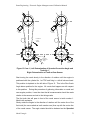
5.4.1
Static setting
72
5.4.1.1 Case 1 No missing teeth on crank and one cam tooth
72
5.4.1.2 Case 2 Missing teeth on crank and no cam sprocket
75
Condition A when crank sensor points at a sector with no missing teeth
75
Condition B when crank sensor points inside the sector containing the
missing teeth
77
5.4.1.3 Case 3 No crank sprocket and with missing teeth on cam
sprocket 79
Condition A when cam sensor points at a sector with no missing teeth
79
Condition B when cam sensor points inside the sector containing the
missing teeth
82
5.4.1.4 Case 4 No crank sprocket and with distributor
83
5.4.2
Dynamic setting
84
Case 1 Engines with no missing teeth on crank sprocket and one cam
tooth
85
Case 2 Engines with missing teeth on crank sprocket and no cam
sprocket
85
Case 3 Engines with no crank sprocket and with missing teeth on cam
sprocket
85
Case 4 Engines with no crank sprocket and number of teeth on cam
equal to “Number of Cylinders” with distributor
86
5.5
Fuel injection setup
86
5.6
Harness Wiring
86
5
6
GLOSSARY
89
6
Reata Engineering, Electronic Engine Management and Calibration Manual
1 Introduction
This manual is intended to provide a brief overview on engine tuning, a
detailed description of the Reata Engineering Graphical User Interface (GUI),
and ECU wiring information. Readers that are new to engine tuning should
find the first chapters informative and are advised to read through them.
Experienced tuners can go to the GUI and wiring chapters immediately.
2 ECU basics
The Engine Control Unit is used to control the operation of internal
combustion engines. Typically this involves the control of fuel quantity and
spark timing as well as other ancillary controls. The ECU is a microprocessor
based electronic circuit that is capable of executing its code at very high
speeds and thus able to monitor and control the engine to crank angle
resolution.
The ECU operates off look-up tables to determine the appropriate value of
fuel quantity and spark timing.
The look-up tables would usually be
determined through experiment on the same engine.
2.1 ECU, Sensing
The ECU requires knowledge on the engine status in regards to its crank
angle, engine rpm, engine load (determined through Manifold Absolute
Pressure or Throttle Position Sensor), coolant temperature, air temperature,
Exhaust Oxygen (Lambda) sensor etc. The sensors used are not unique and
vary due to make and year of production. However some general description
on the sensors can be drawn.
Crank and Cam Sensors
The function of the crank and cam sensors is to provide knowledge of angular
position and speed of the engine to the ECU. The ECU requires knowledge
of angular position of the engine crank so that spark and fuel are generated at
Mario Farrugia
7
Reata Engineering, Electronic Engine Management and Calibration Manual
the desired crank angle. (details of the different crank and cam sensor
configurations can be found in Appendix 5.4 ‘General Engine Settings,
Overview’ )
Usually these sensors are inductive type, two wire (or three wire) and operate
on the principle that a voltage is generated in a coil when iron (a tooth) goes
past the sensor at some speed. Other types of position sensing is sometimes
used such as optical triggering or hall effect (hall effect requires use of
magnets).
Manifold Absolute Pressure (MAP)
The MAP sensor is used to provide intake manifold pressure measurement
which can be used as an engine load indicator.
Sometimes this is also
referred to as Manifold Air Pressure, however the use of the word Absolute is
more descriptive as it has to be appreciated that the pressure being measured
is not gauge but absolute.
Note that gauge pressure refers to pressure
quantity above atmospheric pressure. Ambient pressure is 100kPa (14.7 psi)
in an absolute scale and not zero.
MAP sensors are typically three wire
(ground, signal and supply) and vary in their pressure measuring range
depending on application. Naturally aspirated engines typically utilise 100kPa
sensors while turbocharged (or supercharged) engines utilize 200kPa or
300kPa sensors.
Throttle Position Sensor (TPS)
Usually a potentiometer directly connected to throttle body’s butterfly shaft.
The overall electrical resistance of the potentiometer can vary from one
sensor to another. However the overall resistance has practically no effect on
the throttle position measurement. The ECU reads the voltage at the wiper
which is a function of the orientation (angular position) of the shaft.
Coolant and Air temperature
The coolant and air temperature sensors are usually thermistors. Thermistors
are resistors whose resistance changes with temperature.
Mario Farrugia
Used in
8
Reata Engineering, Electronic Engine Management and Calibration Manual
conjunction with a pull-up resistor, the thermistors and pull-up resistor make a
potential divider whose voltage output depends on temperature. The voltage
is read by the ECU to provide temperature measurement. The thermistor has
two electrical terminals and therefore two connections to the harness,
however sometimes the coolant temperature sensor has one side of the
thermistor grounded to the engine and hence the sensor will have only one
electrical terminal.
Oxygen (Lambda) sensor
This sensor has seen a lot of evolution over the years. The fundamental
principle is based on the production of a voltage by zirconium dioxide element
when exposed to fresh air and exhaust gas. The most basic sensor is the
one-wire sensor. The single wire provides a voltage that changes in relation
to exhaust oxygen. The output signal of the single wire sensor referenced to
chassis ground. The two-wire sensor provides two electrical connections one
for ground and the other for signal. Therefore the two-wire has better signal
quality compared to the one-wire (note that the single wire’s ground
connection to the chassis is through the possibly rusted exhaust system ).
Oxygen sensors require an operational temperature above 300°C to function
properly. The three-wire senor has an embedded heater that heats up the
sensor quickly on start-up thus enabling a much faster knowledge of exhaust
oxygen. In a three-wire sensor, usually two wires are for the heater (typically
two white wires) and the third is signal (referenced to chassis ground). A fourwire sensor has two wires for heater (typically two white wires) and the other
two wires are signal and signal ground. One, two, three and four wire sensors
provide a voltage ranging from zero to 1Volt. A voltage of approximately 0.45
volts indicates stoichiometric condition, voltages lower than 0.45 imply lean
combustion while voltages higher than 0.45 imply rich combustion.
The
measured voltage cannot provide knowledge on the Air to Fuel Ratio AFR but
only knowledge whether rich or lean. Five-wire sensors do provide a voltage
that provides knowledge on the AFR. Five-wire sensors are also referred to
as wide- band sensors. Wide band sensors have signal conditioning circuitry
and provide a linearized voltage output with AFR.
Mario Farrugia
9
Reata Engineering, Electronic Engine Management and Calibration Manual
2.2 ECU, Electronic Control
The ECU controls the engine through fuel injection and spark timing. For
spark ignition engines, the quantity of fuel required is in direct proportion to
the quantity of air inhaled by the engine. The mass of Air to mass of Fuel
ratio (AFR) for ideal operation is stoichiometric. When a three way catalytic
converter is used in production vehicles, the AFR is cycled (through closed
loop control) between rich and lean in order for the catalyst to be able to
perform both oxidizing and reduction reactions.
In racing applications the
AFR is typically maintained rich (that is AFR smaller than AFR stoichiometric)
because this produces more power and is safer for the engine.
2.2.1
Fuel Injection
Spark ignition engines operate at AFR close to stoichiometric. The quantity of
fuel required to obtain the required AFR is controlled by the amount of time
the injector is left open, and is referred to here as Duration Of Injection (DOI).
The DOI required at any condition depends mostly on Volumetric Efficiency
which in turn is very dependent on engine rpm. The DOI required is also
dependent on engine load which is determined through the MAP or TPS
sensors. It is noted here that the logical consumption of much more fuel at
higher rpm is due to the fact that the DOI applicable is injected every
revolution (or every other revolution). Fuel injectors are very quick-acting onoff valves capable of being cycled (that is opened and closed) in the order of a
millisecond. Injectors are available in a variety of flow rates and are also
divided into low impedance and high impedance injectors depending on their
electrical resistance. Peak-and–hold drivers can drive both low impedance
and high impedance injectors while saturation drivers can drive high
impedance injectors only.
2.2.2
Spark Generation
The timing of the spark is critical for optimal engine operation. Typically spark
timing has to be advanced with increasing engine rpm. This is due to the fact
that spark has to be generated in an earlier crank angle if the flame front is to
Mario Farrugia
10
Reata Engineering, Electronic Engine Management and Calibration Manual
travel across the combustion chamber at higher rpm while still fully
combusting all gases just several degrees after top dead centre. The optimal
spark timing is also dependent on engine load. Lighter engine loads require
more advanced spark due to a slower moving flame in lower density
combustion gases. In older mechanical systems this spark advance at low
engine loads was achieved by the vacuum advance system. Various types of
spark generation and delivery are available, namely, one coil with distributor,
a coil every two cylinders (wasted spark) and an individual coil for each
cylinder. The spark, as with the older contact breaker setup (make and break)
is generated by the switching-off of current to the coil. This is so because the
coil (inductor) cannot allow the magnetic flux to vanish immediately and
therefore a high voltage is produced which is capable of producing an
electrical discharge across the spark plug gap. The Capacitive Discharge
Ignition (CDI) delivers a quantity of electricity to the coil at a very high voltage
on the primary side of the coil (can be 300V).
This high voltage in CDI
systems charges the coil a lot faster and leaves enough time to recharge and
spark the plugs more than once per engine cycle (multi spark).
3 Using the ECU
The ECU is an electronic circuit using state of the art microprocessor,
memory, signal conditioning and power transistors.
The wiring diagram
should be well followed before connecting power to the system. Damage to
the ECU can be done if wiring is not correct or not following the wiring
suggestions. This applies most of all to making sure that ECU pins that are
supposed to be connected to power are correctly connected to the relevant
power, while pins that are not supposed to be supplied with power aren’t
connected to power. It is also worthwhile mentioning that high voltage spikes
(around 350V) are generated by the spark plug coils even on the low voltage
side (that is ECU side). These high voltage spikes are properly handled by
the coil drivers but should not be connected to any other ECU pins other than
the coil drivers.
Before using the ECU, the wiring strategy must be developed. The attached
wiring diagram should be used as the basis of the strategy, with modifications
Mario Farrugia
11
Reata Engineering, Electronic Engine Management and Calibration Manual
as necessary for the particular user application such as fuses, starting,
charging and other ancillary circuits.
3.1 Usual Wiring Information and
Commonalities
ECU’s are powered from battery voltage, nominally 12V. The battery voltage
is not actually 12V all the time as during cranking voltage will surely drop,
while during charging voltage would be around 13.8V. The spark plug coils,
injectors, oxygen sensor heater, relays, dashboard indicator lights and other
ancillaries will typically run off 12V supply. The ECU internal electronics will
typically run at lower voltage. This voltage was 5V until recently and now is
3.3V. Sensors will also typically be powered by a lower voltage, typically 5V,
however some sensors do get powered by the battery 12V. Sensor signals
are typically between 0 and 5V, one exception is the two wire inductive pickup
(used for crank and cam sensors) whose output voltage increases from less
than a volt at low rpm but can reach as high as 20V depending on application.
Due to the fact that ECU electronics and power electronics have a common
ground but a different high side voltage as described above, switching of the
power circuits by the ECU electronics is achieved by closing or opening the
connection of the power circuits to ground. That is, coils and injectors would
have a continuous 12V supply (battery voltage), the ECU would then turn on
the coils and injections by supplying a ground connection to them. Turning-off
of the power is achieved by breaking the connection to ground.
Such a
strategy was also used in the past on mechanical contact breakers systems.
At this stage it is appropriate to note that due to the fact that all current from
coils, injectors and other power circuits flows into the ECU through the low
voltage side (ECU side) of these power consumers, the ground current
flowing out of the ECU is very high when compared to the much smaller
current flowing into the ECU from the battery positive supply to power the
ECU electronics. This fact needs to be appreciated to recognize why there
are typically many more ground connections compared to the 12V positive
supply connections.
It is advised that all these ground connections are
connected so that there is ample current handling capability.
Mario Farrugia
12
Reata Engineering, Electronic Engine Management and Calibration Manual
Another word on grounds, different types of grounds are cited, namely battery
ground and analogue ground. Battery ground is the ground that is directly
connected to battery, its main feature is its huge current carrying capacity, the
current flowing from coils and injectors would be routed to this ground inside
the ECU.
The analogue ground is the ground that is used by analogue
sensors, analogue meaning voltage that can vary continuously between
ground and supply voltage. Examples of analogue sensors are TPS, MAP
and temperature sensors. The voltage output of these sensors varies in direct
proportion to the measured parameter. Therefore the ground voltage level of
these sensors has to be very stable otherwise a slight shift in the voltage level
of the ground would be erroneously translated into a change in the measured
parameter value. It should be noted that battery ground would have discrete
shifts in ground voltage level due to the turning on and off of coils and
injectors and turning on and off of other digital electronics. A filter to cancel
these shifts in ground level is typically employed to produce a clean analogue
ground. The supply voltage to the analogue sensors (typically 5V) would also
be a clean voltage, that is it would also be without any voltage shifts due to
switching. Appreciating the differences between these ground and supplies is
important so that connections are made to the appropriate terminals and not
just by whatever happens to seem the easiest physical connection on the
vehicle.
Heat dissipation: Electronic circuits do need to get cooled and cannot operate
at high temperatures. The ECU heats up in part due to the microcontroller
and associated electronics but mostly due to the power transistors associated
with switching on and off of the coils, injectors and other auxiliaries. The
reason behind the heat generated by power transistors is due to the fact that
when switched on, the power transistors would have a voltage drop across
them say of 0.8V. Therefore if a coil draws 5Amps in saturation, it would
translate in 4W (P=IV, P=5*0.8=4) of heat generated in the transistor that has
to be dissipated into the surroundings. Therefore ECU’s typically have there
case that functions as a heat sink for the internal electronics. To make sure
the heat sinking is effective, the ECU should be mounted in a relatively cool
location and if possible have air current or mounted to heat sinking (and cold)
metal parts.
Mario Farrugia
13
Reata Engineering, Electronic Engine Management and Calibration Manual
3.2 Engine Calibration
In this section on engine calibration a strategy is described to map an engine
even if no knowledge of injector DOI is known beforehand.
Simple
calculations of injection duration are suggested to provide a baseline fuel
table from which the engine could be started, and then fuel tables are fine
tuned by experiment. Similar baseline numbers for ignition timing are given.
Experimental dynamometer testing would then usually be the next logical step
to determine spark/fuel hooks, MBT timing and whether to inject onto open or
closed intake valves.
Since the fuel quantities for a new application might be significantly different
from other applications which the end user might have encountered, the lookup tables must be generated from a clean sheet.
A simple process for
generating fuel tables will be described herein.
3.2.1
Getting started with a new engine
This manual describes a process used to calibrate the settings for an engine
which is new to the end user. It is assumed that at this point an engine and
programmable ECU would have already been committed.
The calibration
process here is described by giving reference and going through the process
as used for calibrating a 600cc Honda motorcycle engine. A simple and
systematic process of establishing and building the spark and fuel tables and
testing of the engine is described. The first priority would be to establish the
baseline fuel table and ignition table with which to start and run the engine.
Engine Details
To get started, some basic engine parameters must be known.
For the
Honda F4i engine used in this study, some of the fundamental engine
parameters are summarized in Table 1 below:
Mario Farrugia
Engine Type
F4i
Bore
67.0 mm
Stroke
42.5 mm
14
Reata Engineering, Electronic Engine Management and Calibration Manual
Engine Displacement
599 cc
Compression Ratio
12:1
Firing Order
1-2-4-3
Idle speed
1300rpm
Table 1 Honda CBR600 F4i Parameters [Honda User’s Manual]
3.2.2
Injection Table
Before starting the engine, some initial calculations need to be performed to
establish a preliminary fuel look-up table. The approach is to calculate how
much fuel would be necessary for stoichiometric combustion in each cylinder,
assuming that each cylinder is filled with air at atmospheric pressure (100%
volumetric efficiency). The fuel quantity for idle conditions is then calculated
for an expected typical MAP value at idle.
For one cylinder of 150cc filled with air (only) at 100kPa and 20°C (293K),
using the Ideal Gas Law we have
Mass of air = ma =
PV 100 × 10 3 Pa ⋅ 150 × 10 −6 m 3
=
J
RT
287
⋅ 293K
kg ⋅ K
= 1.78 × 10 − 4 kg
Next, if the stoichiometric air-to-fuel ratio is 14.5, then the mass of fuel
required per cylinder per cycle would be,
ma
1.78 × 10 −4 kg
=
AFR
14.5
= 1.23 × 10 −5 kg
Mass of fuel = m f =
For gasoline of Specific Gravity of 0.75 [Heywood, Internal Combustion
Engine Fundamentals]
1.23 × 10 −5 kg
kg
0.735
l
−5
= 1.64 × 10 l
= 0.0164ml
Volume of fuel = V f =
Mario Farrugia
15
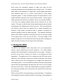
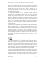
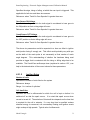
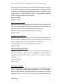
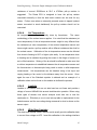
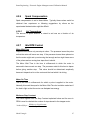
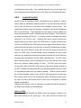
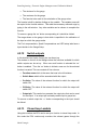
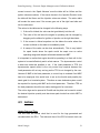
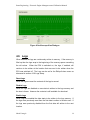
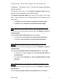
Reata Engineering, Electronic Engine Management and Calibration Manual
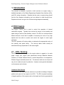
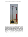
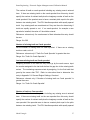
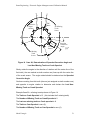
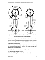
Figure 1 Injector Flow Test
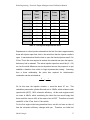
As an example the flow test from the Honda 600F4i stock injectors is detailed.
The flow rate was measured by pulsing the injectors for 8ms, while counting
the number of injection events, and measuring the total volume of fuel
collected in a graduated cylinder. Table 2 shows the fuel injector calibration
measurements. A fuel flow bench feature is implemented in the Reata ECU
specifically for this kind of test (in GUI: Diagnostics, Fuel, Flow test). The
average volume for the injectors was 0.0280 ml per 8 ms pulse.
Mario Farrugia
16
Reata Engineering, Electronic Engine Management and Calibration Manual
Fuel
Injector #
Press
[psi]
Volume
Pulse
[ml]
Count
Flow
[ml /8
ms]
1 run 1
50
77
2719
0.0283
1 run 2
50
78
2749
0.0284
2 run 1
50
78.5
2827
0.0278
2 run 2
50
78
2790
0.0280
3 run 1
50
79
2867
0.0275
3 run 2
50
79
2877
0.0275
4 run 1
50
77
2732
0.0282
4 run 2
50
78
2758
0.0283
Table 2 Fuel Injector Experimental Data
Experiments on other injectors showed that the fuel flow rate is approximately
linear with injector open time, that is, the actual time that the injector needle is
open. It was determined that the time to open the Honda injectors was 0.2 to
0.5ms. This is the time required to activate the solenoid and open the injector,
before any fuel is released. The actual injection open time would be (8 – 0.5)
ms, but the small difference was not important here as the purpose is to just
establish a baseline from which to begin dynamometer testing. Assuming
then a linear relationship, the pulse time required for stoichiometric
combustion can be calculated as:
8
x
=
0.0280 0.0164
So, for this case, the injection duration, x, would be about 4.7 ms.
This
calculation presumed a cylinder filled with air at 100kPa, which relates to wide
open throttle (WOT), 100% volumetric efficiency. At idle most engines would
run close to 40kPa, which considering the Ideal Gas Law would imply that
there would be close to 40% of the mass of air at WOT. Therefore we would
need 40% of the 4.7ms, that is 1.9ms at idle.
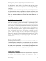
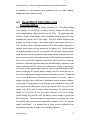
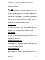
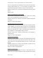
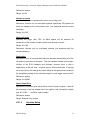
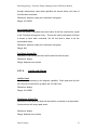
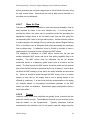
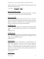
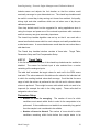
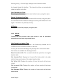
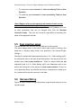
For the first engine trials being described here, we did not have an idea of
how the volumetric efficiency changes with rpm. Therefore, our initial fuel
Mario Farrugia
17
Reata Engineering, Electronic Engine Management and Calibration Manual
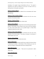
table was only a function of load. That is, our fuel injection duration was
4.7ms at WOT for all speeds, and 1.9ms at zero throttle for all speeds. The
intermediate throttle positions were linearly interpolated between these end
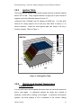
values. The initial fuel table is shown in Figure 1, which is in the form of a
wedge. It is not dependent on speed, simply 1.9ms at zero throttle and 4.7ms
at WOT.
Fuel
4.50-5.00
5.00
4.00-4.50
4.50
3.50-4.00
3.00-3.50
4.00
2.50-3.00
3.50
2.00-2.50
fuel (ms) 3.00
1.50-2.00
1.00-1.50
2.50
20
0
10000
8000
4000
tps %
2000
100 80
60 40
0
1.00
6500
1.50
13000
2.00
rpm
Figure 2 Initial Fuel Table
The load parameter shown in Figure 2 is TPS, however the calculations were
based on a load condition described by MAP in kPa. This equivalence in
description of no-load as 40kPa in a MAP based table and 0% in a TPS based
table is fine. The same applies to full load condition, where this is described
by 100kPa in a MAP based table (naturally aspirated) and 100% TPS in TPS
based table. However the linear relationship, described by the slope of Figure
2 is only really applicable to a MAP based table. The MAP value produced at
a specific TPS opening, it not constant with engine rpm and this would effect
the fuel requirement. Nonetheless Figure 2 is a valid initial table from where
the engine can be started.
Mario Farrugia
18
Reata Engineering, Electronic Engine Management and Calibration Manual
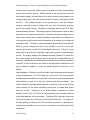
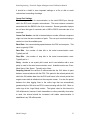
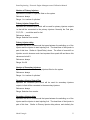
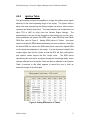
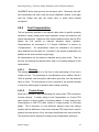
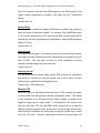
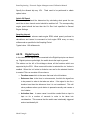
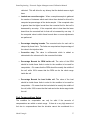
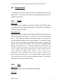
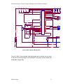
3.2.3
Ignition Table
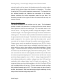
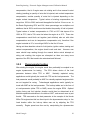
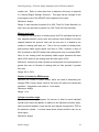
The Honda Service Manual states that the spark advance is thirteen degrees
before TDC at idle. Thirty degrees advance at high rpm is quite normal for
engines; hence the initial table was set to have 13°
advance at idle (1300rpm) and 30° advance at 6000 rpm. It is also quite
common for racing engines not to have any load offset to timing i.e. no
vacuum advance.
Hence the initial ignition table was setup to be only a
function of speed. Refer to Figure 3.
35.0-40.0
30.0-35.0
IGNITION
25.0-30.0
40.0
35.0
30.0
20.0-25.0
15.0-20.0
10.0-15.0
5.0-10.0
25.0
0.0-5.0
Ignition
20.0 Advance
15.0
(Deg)
10.0
5.0
100
80
60
40
tps %
20
13000
11000
9000
8000
7000
6000
4000
0
+
2000
0.0
rpm
Figure 3 Initial Ignition Table
3.2.4
Starting and Coolant Temperature
Compensation
It is very well known and accepted that some extra fuel would be required to
start a cold engine.
In carburettor systems the choke, be it manual or
automatic, would help in starting a cold engine. In electronic fuel injection
systems, this extra quantity of fuel is attributed to two causes: starting
Mario Farrugia
19
Reata Engineering, Electronic Engine Management and Calibration Manual
compensation, that is if engine was not rotating and is then sensed to start
rotating (cranking) a quantity of extra fuel is injected; and coolant temperature
compensation, another quantity of extra fuel is injected depending on the
engine coolant temperature.
Typical values of starting compensation can
range from 150% to 200% and would be applied for the first 10 turns or so. In
the Reata Engineering ECU and GUI, these percentages are multipliers not
additions, that is 200% would mean that double the quantity of fuel is injected.
Typical values of coolant compensation is 170% at 10°C that tapers off to
100% at 70°C, that is 70% extra fuel when the engine is at 10°C. These two
compensations would both act together (and definitely also act with other
compensations such as air temperature compensation etc), therefore if the
engine is started at 10°c, is would get 340% for the first 10 turns.
Having set these baseline values for fuel injection, ignition values, starting and
coolant compensations, the engine should crank and start. However new
users should keep reading through the manual before actual attempts at
wiring and cranking the engine are attempted as there are many more
aspects of the ECU that need to be understood and followed.
3.2.5
Dynamometer testing
After starting the engine, the engine would then preferably be coupled to an
engine dynamometer for testing.
The ECU allows choice of the load
parameter between either TPS or MAP.
Naturally aspirated racing
applications would typically be tuned with TPS as the load parameter. The
load parameter would probably be MAP for naturally-aspirated engines which
are not targeted for racing.
Turbocharged applications would typically be
tuned with MAP as the load parameter. The look-up tables are in the form of
a Load parameter (either TPS or MAP) versus the engine RPM. Optimal
ignition timing and fuel injection duration would then be determined at all
available speed discretizations in the table at WOT, and several more at part
throttle. TPS was used as the load parameter in the example of the Honda
600cc F4i engine since this is a direct input in the dynamometer setup, i.e. the
Load location within the look-up tables was set by adjusting the TPS
manually.
Engine speed was then set by manipulating the dynamometer
Mario Farrugia
20
Reata Engineering, Electronic Engine Management and Calibration Manual
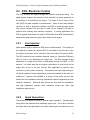
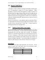
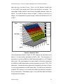
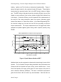
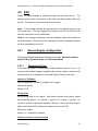
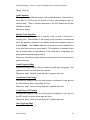
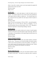
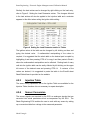
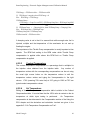
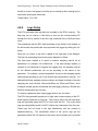
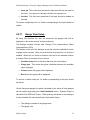
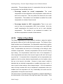
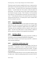
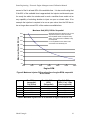
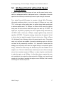
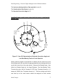
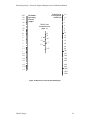
loading. Ignition and Fuel hooks as determined experimentally. Figure 4
shown the spark hooks for the restricted Honda 600 engine. These ignition
hooks show the expected trends, that is the MBT timing is higher at higher
rpm. The MBT timing is high also where the volumetric efficiency is poor (this
relates to vacuum advance, that is when cylinder is lightly filled, advance has
to be larger). Volumetric efficiency can be measured from measurements of
the mass air flow using automotive mass flow sensors, laboratory grade
laminar flow element, or critical flow orifices. In the Reata Engineering ECU,
the load-cell voltage can be read into the GUI thus providing a real–time
torque measurement. The torque measurement can be logged and further
analysed and plotted against ignition timing and/or injection quantity using
Excel®.
Effect of Spark Advance on Torque for various engine speeds
110
3000 rpm
4000 rpm
100
5000 rpm
To rqu e , lb-ft
6000 rpm
90
6500 rpm
8000 rpm
9000 rpm
80
70
60
50
15
20
25
30
35
40
45
50
55
Spark Advance, deg BTDC
Figure 4 Spark Advance Hooks at WOT
Additional tests can be conducted to determine the best timing for start of fuel
injection. For the Honda F4i engine being described, best performance was
measured with fuel injected onto open valves, versus closed valves. It was
found that injection onto open valves gave 6% more torque at the point of
worst volumetric efficiency (6500rpm). This was a worthwhile improvement
given the fact that it did not involve any extra hardware. Note that this can
Mario Farrugia
21
Reata Engineering, Electronic Engine Management and Calibration Manual
only be done if the fuel injection strategy is sequential, that is ECU is
knowledgeable of each cylinder’s strokes. Sequential operation requires a
cam signal into the ECU to reset and synchronize the four stroke cycle,
sequential operation is described in Appendix 5.4 ‘General Engine Settings,
Overview’.
3.2.5.1
Compensations
After dynamometer calibration is finalized, some additional tests would still
need to be done to determine the necessary amounts of compensations. The
compensations that need to be determined are: coolant temperature
compensation, air temperature compensation and throttle pump.
During
dynamometer testing it is important to have the engine in known and stable
operating conditions of coolant and air temperature.
These temperatures
would be the basis from where compensation is applied. That is if coolant
temperature during dynamometer tests was stable between 90 and 100oC
then the coolant compensation table would have to be 100% at the 90 and
100°C region and higher values than 100% at colder temperature. At hotter
coolant temperatures it would be logical to have less than 100% due to the
fact that the air induced into the cylinder would be hotter, hence less dense
and consequently requiring less fuel. However it is usual not to lower the
coolant compensation value below 100% above the baseline operating
temperature in order to help in cooling the engine and keep away from
possible knocking. Coolant compensation should be adjusted so that while
warming up, the engine would operate adequately with an AFR close to the
desired value.
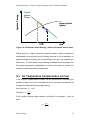
Air temperature compensation would also be applied below and above the
baseline air temperature maintained during dynamometer testing.
For
naturally aspirated engines a fairly constant air temperature during
dynamometer testing can be achieved by ducting air into the engine from
outside the test cell. For the baseline temperature maintained during testing
the air temperature compensation would be 100%. At colder air temperature
the density of the air would be bigger and hence a larger quantity of fuel can
be injected. On the other hand, at hotter air temperatures the air density is
less and hence less fuel can be injected. Due to the fact that it would not be
Mario Farrugia
22
Reata Engineering, Electronic Engine Management and Calibration Manual
quite easy to experimentally vary the inlet air temperature by fairly large
amounts, the best way to calculate the required amount of compensation is
through theory using the Ideal Gas Law.
Refer to Appendix 5.3 ‘Air
Temperature Compensation on Fuel’ for the derivation and quantification of
air temperature compensation.
In turbocharged applications the air temperature (usually measured
downstream of the turbocharger) depends heavily on the turbo operating
condition, that is boost pressure and rpm. Hence in turbo applications the
baseline air temperature is suggested to be taken in the region of preferred
operation of the engine, that is the region in which the car is intended to be
driven.
Such a temperature would typically be higher than atmospheric
conditions, say 50°C and depends on application, especially boost pressure
and intercooler size.
The throttle pump compensation injects additional fuel when the accelerator
pedal is depressed quickly. The electronic throttle pump facility in ECU’s
mimics the mechanical throttle (or accelerator) pump but gives a much higher
modification capability.
The quantity of extra fuel required will vary from
application to application and would have to be finally tweaked during driving.
The compensations, including the equations on which the throttle pump
compensation are calculated, are discussed further in section 4.2.5 ‘Fuel
Compensation’.
4 GUI
The Reata Engineering GUI is a Windows based software and has pull
down menus that are very typical to Windows based applications. The pull
down menus in the Reata Engineering GUI are detailed in this manual in the
same order of appearance in the pull down menus: staring from left to right
and then top down. This simple and structured sequence of description of the
menus is intended to make access to descriptions in this manual easier.
If an ECU is connected and communicating with the computer, then the GUI
will load the Engine Settings File from the ECU. The execution of GUI without
a communicating ECU will prompt a request for the loading of an Engine
Settings File from disk. The entries in the pull down menu can be greyed out,
Mario Farrugia
23
Reata Engineering, Electronic Engine Management and Calibration Manual
this happens if the ECU is not communicating and the particular pull down
menu entry cannot function.
4.1 File
This tab provides management of the Files associated with the ECU. These
files have an extension .esf which stands for engine settings file.
It is
important to appreciate that there are four locations where these settings can
reside namely: disk, GUI, ECU memory and ECU flash.
ECU has both
memory and flash. The ECU displays, executes and saves the settings that
are in memory not in flash. The settings that are stored in flash are only as
backup and must first be loaded to memory to be displayed, executed or
saved. Management of the flash is detailed in section 4.3 subsections Store
Parameters in Flash and Restore Parameters from Flash.
Open Configuration
The Open Configuration tab allows the opening of a saved settings file from
disk. If an ECU is connected to the PC and communicating with the GUI,
using the Open Configuration will only load the GUI with the settings from the
specified file on disk, the ECU will still have the settings it had before.
Save Configuration
The Save Configuration tab saves the current engine settings present in the
GUI to disk. Note that the save feature saves the settings in the GUI and not
the settings in the ECU (if the ECU settings are to be saved they first must be
downloaded from ECU into GUI).
Download Configuration from ECU
The Download Configuration from ECU allows downloading of the engine
settings from the ECU to the GUI on the computer. Note that this tab does
not save the settings to file it only downloads the settings from ECU so that
ECU and GUI are using the same settings.
Upload Configuration to ECU
The Upload Configuration to ECU allows uploading of the engine settings
from the GUI to the ECU. Once this is done the previous settings in the ECU
will be overwritten, however the settings in flash would remain as they were.
Mario Farrugia
24
Reata Engineering, Electronic Engine Management and Calibration Manual
It should be a habit to save important settings to a file on disk to avoid
unintentional overwriting of settings.
Comm Port Settings
The Comm port, short for communication, is the serial RS232 port through
which the ECU and computer communicate. The most common connector
associated with the RS232 is the 9 pin connector. Recent generation laptops
do not have this type of connector and a USB to RS232 converter has to be
employed.
Comm Port Number: set this to the desired port number, different computers
might not have the same numbers of ports. The com port is selected using a
combo box from the available ports.
Baud Rate: the communicating speed between the ECU and computer. This
value is typically 57600.
Data Bits:
the number of data bits in the serial communication word.
Typically set to8.
Stop Bits:
the number of stop bits in the serial communication word.
Typically set to 1.
Parity: whether or not a parity bit is used, and if used whether odd or even
parity is used in the serial communication word. Available entries are: Even;
Mark; None; Odd; Space. Typically set to None.
Sampling Interval: the amount of milliseconds that the GUI allows to pass
between communications with the ECU. This period is the refresh period with
which the GUI obtains data from the ECU and hence is the refresh period that
engine sensor data is refreshed on the computer screen. It is also the period
between the data logging lines in the online logs that are automatically
generated by the GUI when an ECU is communicating with the GUI. More on
online logs in the ‘Logs Setup’ section. The typical value for this interval is
100 milliseconds, however if radio transmitters or other potentially slow setup
is used, the interval should be increased until stable communication is
established, say 300 milliseconds.
Mario Farrugia
25
Reata Engineering, Electronic Engine Management and Calibration Manual
4.2 Edit
Editing of engine settings is effected through this pull down menu.
The
settings screens have two buttons on the right hand side namely: Done and
Cancel. The function of by these buttons is as follows.
Done: if the changes effected are good and they are desired to stay in the
GUI, press Done. This only registers the values in the GUI, the ECU will still
have the values prior to any modification.
Cancel: if the changes effected are not worth keeping, press Cancel and they
will be discarded. The values prior to opening the particular settings interface
will be re-established in the GUI.
4.2.1
General Engine Configuration
The General Engine Settings are divided into four tabs: Mechanical Setup,
Ignition Setup, Injection Setup and Limits and Alarms.
4.2.1.1
Mechanical Setup
In this tab the details of mechanically related settings need to be set. An
overview with related diagrams explaining the various cases an end user will
encounter is given in Appendix 5.4 ‘General Engine Settings, Overview’.
Number of Cylinders
Set the appropriate number of cylinders in the engine.
Relevance: always
Range: 1 to 8
Firing Order
Set the firing order of the engine. Note that the ignition and injector cables
are connected ignition 1 to cylinder 1, ignition 2 to cylinder 2, ignition 3 to
cylinder 3 and so on and same applies to injectors. That is the firing order is
taken care of by the ECU and hence needs to be set in the GUI.
Relevance: always
Range: 1 to ‘Number of Cylinders’
Number of teeth on Crank sprocket
Mario Farrugia
26
Reata Engineering, Electronic Engine Management and Calibration Manual
The number of teeth on crank sprocket including any missing ones is entered
here. If there are missing teeth on the crank sprocket then this entry should
specify the number of existent teeth plus the imaginary number of teeth on the
crank sprocket if the sprocket were to have a constant pitch equal to the pitch
between two existing teeth. The ECU handles sprockets with equally spaced
teeth. Any missing teeth are considered as if they are there for determining if
teeth are equally spaced or not. If no crank sprocket, for example a cam
sprocket is installed, the value of 0 should be entered.
Relevance: relevant only if a crank sensor is fitted otherwise this entry should
be zero.
Range: 0 to 200
Number of missing teeth on Crank sprocket
Set the number of missing teeth on crank sprocket. If there are no missing
teeth on crank, set to 0.
Relevance: relevant only if ‘Teeth On Crank Sprocket’ is greater than two.
Range: 0 to ‘Teeth On Crank Sprocket’-1
Last non-missing tooth on Crank sprocket
Assigning numbers to the teeth as they would go by the crank sensor, input
the number assigned to the last tooth before the gap due to the missing teeth
arrives. The numbering sequence starts by assigning 1 to the first tooth that
goes by the sensor after TDC. Refer to notes about how to determine this
entry in Appendix 5.4 ‘General Engine Settings, Overview’.
Relevance: relevant only if ‘Number of missing teeth on Crank sprocket’ is
greater than zero
Range: 1 to ‘Teeth On Crank Sprocket’
Number of teeth on Cam sprocket
The number of teeth on cam sprocket including any missing ones is entered
here. If there are missing teeth on the cam sprocket then this entry should
specify the number of existent teeth plus the imaginary number of teeth on the
cam sprocket if the sprocket were to have a constant pitch equal to the pitch
between two existing teeth. The ECU handles sprockets with equally spaced
Mario Farrugia
27
Reata Engineering, Electronic Engine Management and Calibration Manual
teeth. Any missing teeth are considered as if they are there for determining if
teeth are equally spaced or not. If no cam sprocket, for example a crank
sprocket with missing teeth is installed, the value of 0 should be entered.
Relevance: relevant only if a cam sensor is fitted otherwise this entry should
be zero.
Range: 0 to 200
Number of missing teeth on Cam sprocket
Set the number of missing teeth on cam sprocket. If there are no missing
teeth on cam, for example just one tooth on cam, set to 0.
Relevance: relevant only if ‘Teeth On Cam Sprocket’ is greater than Number
of Cylinders.
Range: 0 to ‘Teeth On Cam Sprocket’ -1
Last non-missing tooth on Cam sprocket
Assigning numbers to the teeth as they would go by the cam sensor, input the
number assigned to the last tooth before the gap due to the missing teeth
arrives. The numbering sequence starts by assigning 1 to the first tooth that
goes by the sensor after TDC. Refer to notes about how to determine this
entry in Appendix 5.4 ‘General Engine Settings, Overview’.
Relevance: relevant only if ‘Number of missing teeth on Cam sprocket’ is
greater than zero
Range: 0 to ‘Teeth On Cam Sprocket’
Crank tooth at Cam Sensor
Specifies the number assigned to the tooth on the crank sprocket which goes
by the crank sensor after the cam tooth lines up with the cam sensor. See
notes in Appendix 5.4 ‘General Engine Settings, Overview’. on how to assign
this entry.
Relevance: relevant only if ‘Teeth On Crank Sprocket’ is greater than zero
and ‘Teeth On Cam Sprocket’ is equal to one.
Range: 0 to ‘Teeth On Crank Sprocket’*2
Sprocket correction angle
Specifies, in crank angle degrees, the amount of offset which has to be
applied so that zero degrees correspond to exact Top Dead Centre of piston
Mario Farrugia
28
Reata Engineering, Electronic Engine Management and Calibration Manual
number one. Refer to notes about how to determine this entry in Appendix
5.4 ‘General Engine Settings, Overview’. This angle can be changed on the
fly through the use of the ADJUST button adjacent to the value.
Relevance: always
Range: if crank sprocket is present 0 to (360/ ‘Teeth On Crank Sprocket’) or
else if only cam sprocket is present 0 to (180/ ‘Teeth On Cam Sprocket’)
Missing teeth ratio
To determine the occurrence of missing teeth, the ECU calculates the ratio of
time elapsed between current tooth and previous tooth divided by the time
elapsed between the previous tooth and the one prior to it divided by the
number of missing teeth plus one. That is for any number of missing teeth,
and perfectly stable engine speed, this value is 100%. However a value of
60% is advised so that ECU detects the missing tooth even in unsteady RPM.
Note, for one missing tooth and perfectly stable engine operation the lower
value is 50% while for two missing teeth the lower value is 33%.
Relevance: relevant only when ‘Number of missing teeth on Crank sprocket’ is
greater than zero or ‘Number of missing teeth on Cam sprocket’ is greater
than zero.
Range: 0% to 100%
Number of strokes for RPM average
Specifies the number of piston strokes which are used in determining the
average RPM. Using a larger value for this entry will reduce the tachometer
oscillation. Suggested to use value of 1 as a starter.
Relevance: always
Range: 1 to 4
Cylinder correction angle
Specifies, in crank angle degrees, the amount of offset for each individual
cylinder which has to be applied, in addition to the ‘Sprocket correction angle’,
which should be applied in order that the zero degrees correspond to TDC for
the particular cylinder. In normal cases these entries would be zero for an
inline engine.
Relevance: always
Mario Farrugia
29
Reata Engineering, Electronic Engine Management and Calibration Manual
Range: -90 to 90
Load Parameter
This combo box specifies the sensor used as load parameter. Normally this is
either MAP or TPS but can be chosen to be any other analogue input, for
example MAF. Refer to relevant discussion in the ECU Basics and Engine
Calibration sections.
Relevance: always
Missing Tooth Algorithm
Specifies the algorithm, simple or complex, which is used to determine a
missing tooth. Determination of the missing tooth occurrence is determined
as by the algorithm explained in the Missing teeth ratio subsection above is
termed Simple. The Complex algorithm compares the current elapsed time
to the time that occurred a stroke earlier. This algorithm is intended to take
care of slowing down and speeding up of the crank due to compression and
power pulses especially during starting.
Relevance: relevant only when ‘Number of missing teeth on Crank sprocket’ is
greater than zero.
Crank Triggering Edge
Specifies the edge, rising or falling, at which the crank input is triggered. This
applicable for both two and three wire sensors.
Relevance: when ‘Teeth On Crank Sprocket’ is greater than zero
Crank Sensor ON Voltage
Specified the voltage at which the teeth signal is considered to have gone to
the ON position so that a rising edge will occur.
Relevance: when ‘Teeth On Crank Sprocket’ is greater than zero.
Crank Sensor OFF Voltage
Specified the voltage at which the teeth signal is considered to have gone to
the OFF position so that a falling edge will occur.
Relevance: when ‘Teeth On Crank Sprocket’ is greater than zero.
Cam Triggering Edge
Mario Farrugia
30
Reata Engineering, Electronic Engine Management and Calibration Manual
Specifies the edge, rising or falling, at which the cam input is triggered. This
applicable for both two and three wire sensors.
Relevance: when ‘Teeth On Cam Sprocket’ is greater than zero
Cam Sensor ON Voltage
Specified the voltage at which the teeth signal is considered to have gone to
the ON position so that a rising edge will occur.
Relevance: when ‘Teeth On Cam Sprocket’ is greater than zero.
Crank Sensor OFF Voltage
Specified the voltage at which the teeth signal is considered to have gone to
the OFF position so that a falling edge will occur.
Relevance: when ‘Teeth On Cam Sprocket’ is greater than zero.
The above six parameters would be expected to a have an offset in ignition
and injection timing if wrongly set. This offset would probably vary with rpm
as the width of the crank pulse is not necessarily a fixed number of crank
angle degrees.
This understanding of whether the hardware being used
provides a trigger that is consistent with the rising or falling edge has to be
available. The Crank/Cam oscilloscope view (explained in section 4.5.5 ) can
help in the determination of the correct values for these parameters.
4.2.1.2
Ignition Setup
Number of coils
Specifies the number of coils fitted on the system
Relevance: always
Range: 1 to ‘number of cylinders’
Coil dwell time
Specifies the time in milliseconds for which the coil is kept on before it is
switched off so that the spark occurs. It is noted that spark occurs when
current is turned off. The selection of this dwell time depends on the time that
is required for the coil to saturate. If a very long time is specified useless
electrical energy is consumed, coil unnecessary heating, and ignition events
might overlap at high speeds. Typical value 4 milliseconds.
Mario Farrugia
31
Reata Engineering, Electronic Engine Management and Calibration Manual
Relevance: always
Range: 0 to 60
Number of sparks
Specifies the number of sparks which occur in one firing cycle.
Relevance: relevant only on multi-spark systems, specifically CDI systems as
these can charge up the coil extremely fast. (not supported with the current
hardware)
Range: 0 to 255
Sparks off angle
Specifies the angle, after TDC, at which sparks will be switched off
irrespective of the number of sparks which have already occurred.
Range: 0 to 180
Relevance: relevant only on multi-spark systems (not supported with the
current hardware)
Spark delay
Specifies the time in microseconds that pass between the switching off of the
coil and the occurrence of the spark. This is a hardware related time mostly a
function of the ECU hardware and software, however there is also a
dependency on the coil used. A typical value is 180 microseconds. If wrongly
set, a bad value in this setting can cause drifting of the ignition event, however
the rising/falling setting of the crank/cam signal is much bigger cause for drift.
Relevance: always
Range: 0 to 60000
Spark Output Pins
Specifies the connector pins which will be used for Spark Outputs i.e that will
be connected to the low voltage side of the ignition coils. Normally the Spark
pins, S1,S2,S3….., would be used for spark.
Relevance: always
Range: Selection from combo.
4.2.1.3
Mario Farrugia
Injection Setup
32
Reata Engineering, Electronic Engine Management and Calibration Manual
Number of Primary Injectors
Specifies the number of injectors fitted on the system
Relevance: always
Range: 1 to ‘number of cylinders’
Primary Injector Output Pins
Specifies the connector pins which will be used for primary injectors outputs
i.e that will be connected to the primary injectors. Normally the Fuel pins,
F1,F2,F3….., would be used for fuel.
Relevance: always
Range: Selection from combo.
Primary Injector delay
Specifies the time in milliseconds that pass between the switching on of the
injector and the injector to start injecting fuel. The dead-time of the injector is
part of this time. Similar to ‘Spark Delay’ above. The effect of some drift on
injection event is however much less important than spark drift and hence this
values can be left 0.
Relevance: always
Range: 0 to 60
Number of Secondary Injectors
Specifies the number of secondary injectors fitted on the system
Relevance: always
Range: 1 to ‘number of cylinders’
Secondary Injector Output Pins
Specifies the connector pins which will be used for secondary injectors
outputs i.e that will be connected to the secondary injectors.
Relevance: always
Range: Selection from combo.
Secondary Injector delay
Specifies the time in milliseconds that pass between the switching on of the
injector and the injector to start injecting fuel. The dead-time of the injector is
part of this time. Similar to Primary injector delay above, and similarly the
Mario Farrugia
33
Reata Engineering, Electronic Engine Management and Calibration Manual
effect of some drift on injection event is much less important than spark drift
and hence this values can be left 0.
Relevance: always
Range: 0 to 60
Injection angle
Specifies the angle, in crank angle degrees, to which the injection event is
referred. If the ‘Injection angle at’ is set to ‘Start’ then this entry specifies the
crank angle at which the injector is switched on. If the ‘Injection angle at’ is
set to ‘End’ then this entry specifies the crank angle at which the injector is
switched off.
Relevance: always
Range: This entry can be between –360° and +360° fo r sequential operation.
Noting that zero is at TDC when the valves are overlapping.
For non
sequential operation this entry can be between -180° to +180°. Sequential is
described in Appendix 5.4 ‘General Engine Settings, Overview.
Injection angle at
Either start or end of the injection duration can be chosen to provide angular
reference of the injection event with respect to engine crank angle. Refer also
to description on the specification of the ‘Injection Angle’ that will follow in the
Injection Setup tab.
Relevance: always
Number of Strokes for injection
Specifies the number of strokes which must elapse between successive
injection events. This feature can be used with single point injection systems
in order to even out the fuel delivery to each of the cylinders. For example, on
a four cylinder engine with single point injection, injecting fuel every 3 strokes
will tend to even out delivery to all cylinders in the long term.
Relevance: always
Range: 1 to 4
Max Percentage Duty Cycle
Specifies, as a percentage of one full cycle, the maximum duration for which
the injector can stay open. The injector has a dead-time which is needed to
Mario Farrugia
34
Reata Engineering, Electronic Engine Management and Calibration Manual
open and close. If the duration of the injection starts to approach the duration
of one whole cycle, then the injector will not be opening for the duration that it
is intended to. When this limit is approached it should be considered to either
fit larger injectors of install secondary injectors. Further details in appendix
section 5.1 Maximum value of DOI for engine
Relevance: always
Range: 0 to 100
Primary injector flow rate
Specifies the flow rate in pounds per hour (lb/hr) for the primary injectors.
This value should be obtained either from the manufacturer of the injectors or
by performing the injector flow test as described in section 3.2.2.
Relevance: when number of secondary injectors is not zero
Range: 0 to 600
Secondary injector flow rate
Specifies, the flow rate in pounds per hour (lb/hr) for the secondary injectors.
This value should be obtained either from the manufacturer of the injectors or
by performing the injector flow test as described in section 3.2.2.
Relevance: when number of secondary injectors is not zero
Range: 0 to 600
Time for Fuel Pump On at boot
Specifies, in seconds, the duration for which the pump is kept on when the
ECU is switched on.
When the ECU is switched on the fuel pump is
energized so that when the engine is started the fuel pressure is already
available.
Relevance: always
Range: 0 to 60
Fuel tank running time
This is useful in cars with fuel tanks without gauges or with irregular shaped
tanks for which level gauges might not mean much.
The ECU keeps a
counter of the quantity of fuel being consumed, by summing the total time of
all injection events. The Fuel tank running time is an empirical (obtained
Mario Farrugia
35
Reata Engineering, Electronic Engine Management and Calibration Manual
through experiments) value which specifies the amount when a full tank of
fuel has been consumed.
Relevance: when an output pin is used as a fuel gauge.
Range: 0 to 65536
Accumulated button
When this button is pressed the current value of the fuel consumed is copied
to the ‘Fuel tank running time’ entry. This can be used so that when a full tank
is known to have been consumed, the full fuel tank is taken to be the
accumulated value.
Relevance: when an output pin is used as a fuel gauge.
Range: N/A
Fuel Pump Output Pin
Specifies the connector pins which will be used for the fuel pump.
Relevance: always
Range: Selection from combo.
4.2.1.4
Limits and Alarms
Cut Rev Limit
Set this value according to the engine’s capability. Both spark and fuel are
cut if the rpm are sensed to go above the ‘Cut Rev Limit’.
Relevance: always
Range: 0 to 20000
Tachometer Output Pin
Specifies the connector pin which will be used for connection to a tachometer.
A pulse occurs with every spark event.
Relevance: always
Range: Selection from combo.
Mario Farrugia
36
Reata Engineering, Electronic Engine Management and Calibration Manual
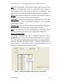
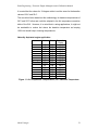
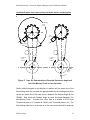
4.2.2
Ignition Table
The ignition table provides the capability to change the ignition values (spark
advance) for the whole operating range of the engine. The ignition table is
setup with rows representing the different engine rpm points, while columns
represent the different load points. The load parameter can be selected to be
either TPS or MAP (or other) from the General Engine Settings.
The
discretization of the rpm can be changed by right clicking on any rpm entry,
three possibilities will appear Edit RPM Value, Insert RPM Row and Delete
RPM Row, refer to Figure 5
Setting RPM entries in Tables.
Use these
options to modify the RPM values representing the rows as desired. Note that
the bottom RPM row value is the RPM value that is used as the highest RPM
on the tachometer displayed on the screen. It is also important to specify this
number higher than the Rev Limiter so that the ECU will have valid ignition
and injection values beyond the Rev Limiter value.
The RPM values
representing the rows will be consistent throughout the settings tables, that is
changes effected from the Ignition Table will also be effected in the Injection
Table, a reminder to this effect appears to remind the user of such an
automatic change in the other table.
Figure 5 Setting RPM entries in Tables
Mario Farrugia
37
Reata Engineering, Electronic Engine Management and Calibration Manual
Similarly the load entries can be changed by right clicking on the load entry,
refer to Figure 6 Setting the Load Parameter entries. The changes effected
in the load entries will also be applied to the injection table and a reminder
appears to this effect when exiting the ignition table editing.
Figure 6 Setting the Load Parameter entries in Tables
The ignition values in the table can be changed by left clicking on them and
typing the desired value.
If mathematical manipulating of the values is
required, it is suggested that the whole table or the desired part is copied by
highlighting it and then pressing CTRL+C to copy it and then paste in Excel
where the mathematical manipulation can be effected. Pasting back of many
cells into the ignition table can be easily effected by left clicking on the upper
left corner of the desired area and pressing CTRL+V.
If contours of the
values are desired, it is suggested to paste the table in the Excel® sheet
ReataTablesView.xls provided on the website.
4.2.3
Injection Table
The same editing capabilities as for the Ignition Table are available for the
Injection Table, therefore it is not necessary to repeat description.
4.2.4
Sensor Conversion
The sensor signals are acquired by the ECU as analogue signals that are
converted into actual parameters such as temperature by the ECU.
The
Reata Engineering ECU enables the user to work with any sensor by setting
up a conversion table from voltage to the measured parameter.
Mario Farrugia
38
Reata Engineering, Electronic Engine Management and Calibration Manual
A sensor can be connected to any analogue input pin. The analogue input
pins are pins marked A01 to A22.
A01, A02, A03 and A04 are inputs which are not amplified.
These are
normally used for TPS, MAP, coolant temp and air Temp.
A05 and A06 are single ended inputs which can be assigned with an
amplification.
A07, A08, A09, A10, A11, A12, A13, A14, A15, A16, A17, A18 are inputs
which can be used as single ended as well as differential inputs. These pins,
in both configurations, can be assigned with an amplification depending on
their setup.
These inputs, taken in pairs, can be used to connect to
thermocouples.
A19 is hard-wired as cam sensor.
A20 is hard-wired as crank sensor.
A21 and A22 are for future use and will be assigned to knock sensors.
Add
Choosing this entry in the Sensor Conversion pull-down menu will enable the
user to create a senor entry and connect it to an input pin.
When a new sensor is created the new entry will be shown in the ‘Sensor
Conversion’ pull-down menu. The user can enter and edit the desired sensor
by clicking on the appropriate entry in the menu.
Delete
A combo box is displayed from which the user can select the sensor input that
he wants to delete.
Edit
By clicking on any of the sensor conversion entries shown in the sensor
conversion pull-down menu the user can enter the edit dialogue for the
relevant sensor.
The dialogue consists of:
Sensor Name: The name to be given to this particular sensor.
Units: The units of measurement for this particular sensor.
Mario Farrugia
39
Reata Engineering, Electronic Engine Management and Calibration Manual
Filter is a number between 1 and 16 which is used to filter out noise that may
be present on the signal input. A value of 1 means that no filter is applied. A
value between 2 and 16 means that the signal will be smoothed out. The
bigger the value the smoother the signal but also the slower the response.
Input pin This combo box specifies the connector pins which will be used for
this sensor. Any pin which is already used is greyed out.
Amplification this combo box specified the amplification which will be used
with this sensor.
Only the appropriate amplifications will be available
according the pin chosen.
Thermocouple if this input is to be used as a thermocouple the type should
be chosen here, otherwise ‘Not thermocouple’ should be selected.
Input If the selected pin can be set as differential, a radio button will be
shown so that the input can either be set to single-ended or differential.
Sensor Conversion Table
The sensor conversion table can be generated using the ECU in
CALIBRATE mode. This feature facilitates the generation of the conversion
table. The right mouse button should be used on the left ‘Voltage’ column to
edit, insert and delete rows. Refer to Figure 7 Setting the Voltage entries in
Sensor Conversion These right mouse button options are identical to those
provided for editing the ignition and injection tables.
Figure 7 Setting the Voltage entries in Sensor Conversion
Mario Farrugia
40
Reata Engineering, Electronic Engine Management and Calibration Manual
An Excel sheet with an example of the test measurements and conversion
of a thermistor sensor is made available on the web site. This Excel sheet
should be of help as thermistors are logarithmic in nature and the use of the
appropriate logarithmic equation makes the conversion table a lot better.
4.2.4.1
Throttle Position
Since the throttle position sensor is usually a linear sensor the extremities of
the sensor travel are usually enough for the conversion table. It is important
to note that if the TPS is mechanically moved in relation to the throttle butterfly
shaft, the calibration may be lost and would necessitate recalibration of the
fuel and possibly ignition tables. The suggested calibration procedure is to
fully close the throttle, fully retracting any idle screw, try to make the throttle
plate rest against the throttle body, then read the voltage input into the ECU
using the CALIBRATE button. Set the value for this voltage to 2 or 3 percent.
Next open the throttle fully, set this as 95 to 97 %. Then set zero volts to 0%
and 5volts to 100%. Such a method would make sure that even if due to
noise a voltage lower than the fully closed voltage enters the ECU, the ECU
will never get confused and interpret that as a percentage lower than zero.
Same thinking applies to the 100% position.
4.2.4.2
Manifold Absolute Pressure
In order to run the calibration a method of pulling a vacuum say down to
30kPa is required. If the engine application is turbocharged the MAP sensor
would also have to be calibrated to 200kPa or 300kPa depending on the
boost level.
A manual vacuum pump with a vacuum pressure gauge is
probably the best method for the calibration below atmospheric pressure. The
atmospheric pressure needs to be measured by means of a barometer to give
a reference value to which the vacuum and gauge pressures are subtracted
and added respectively. In the case a barometer is not available, 100kPa can
be used as a ball-park value or the atmospheric pressure obtained from a
weather station report. Once again it is advised to set the zero volt and five
volt calibration points to MAP values even if these voltages are never reached
during calibration. Plotting of the calibration in Excel® is suggested as MAP
sensors are usually of a linear nature and hence plotting and passing a linear
Mario Farrugia
41
Reata Engineering, Electronic Engine Management and Calibration Manual
trend-line through the measurements should make the calibration curve
neater. If the trend-line is plotted, extend it to zero volts and five volts and use
these as the extreme values for the look-up table. If Excel® cannot be used,
the same procedure can be made manually on graph paper or perform mental
determination of adequate 0V and 5V MAP values. A calibration sheet for a
MAP sensor is available on the website to facilitate understanding of this
procedure. It is also wise to appreciate that the ignition and injection tables
should have a column for the lowest and highest possible MAP value in the
MAP conversion table. This would make sure that even if a voltage outside
usual operation is received by the ECU this still results in a quantifiable value
of ignition and injection.
4.2.4.3
Coolant Temperature
Coolant temperature sensors are typically thermistors.
The calibration
experiment can be easily done by starting with iced water and raising its
temperature up to boiling. A thermometer or thermocouple is required to be
able to determine the temperature of the water. The water ice mix has to be
quite high on ice and crushed ice is better than one big lump of ice. Stirring
throughout the calibration is advised to have a uniform temperature
throughout, calibration every 20°C or so is suggested, heating slowly to go
from one point to the next, and stop heating to read measurements and allow
stirring to reach a uniform temperature. The GUI interface can be used during
the calibration to facilitate the experiment. Temperatures below 0°Celcius and
above 100°Celcius are difficult to obtain and hence a proper extrapolation
method for the thermistor curve should be employed.
Thermistor
characteristics are modelled by the Steinhart equation and this model should
be adopted for proper interpolation and extrapolation. Since characteristic is
not linear, points every 10°C are suggested to be provided in the look-up
table. Please refer to the downloadable Excel Sheet detailing an example of
a coolant sensor calibration. It is also noted that since the thermistor is not
the only resistor in the sensing system, it is suggested to know and account
for the other resistors in the network to obtain the most accurate look-up table.
A proper choice of the pull-up resister is required to provide a full range of
measurements from below 0°C to above 100°C, for a thermistor having a
Mario Farrugia
42
Reata Engineering, Electronic Engine Management and Calibration Manual
resistance of around 2500Ohms at 20°C a 470Ohm pull-up resistor is
suggested.
The Reata ECU is designed to have the pull-up resistor
connected externally so that the best match resistor can be used for any
sensor. Further more when an externally powered sensor is tapped (coolant
sensor connected to stock dashboard) the pull-up resistor should not be
connected.
4.2.4.4
Air Temperature
Air temperature sensing is typically done by thermistors.
The same
methodology of the coolant sensor applies. It is noted that the resistance (at
room temperature) of the air temperature sensor might be very different than
the resistance (at room temperature) of the coolant temperature sensor and
hence might require a pull-up resister with a different resistance than that for
the coolant sensor. Calibration of the air temperature sensor can be effected
from close to freezing to 80°C or higher quite easily. An air temperature close
to freezing can be obtained by putting the sensor in the fridge or freezer or in
an ice filled container. Stirring of the air should be effected to make sure that
a uniform temperature is established between the air temperature sensor and
the thermometer or thermocouple being used to make a valid temperature
measurement.
Hot temperatures can be obtained using a hair dryer and
varying heating or fan control or the distance away from the sensor. Once
again the use of the Steinhart equation is advised and an example of a
calibration sheet can be found on the website to facilitate the process.
4.2.4.5
Lambda
Lambda or O2 sensors that are not wide band are not linear and provide a
voltage of around 450milliVolts around stoichiometric operation. When using
these types of sensors one cannot interpret much how rich or lean the
combustion is. Effectively a one to one look-up table is implemented for the
lambda sensor and the raw voltage being measured is what is shown as the
sensor output.
4.2.4.6
Wide Band Lambda
The wide band lambda sensor manual would usually provide calibration data
to convert from voltage to AFR. Insert this calibration in the settings interface
Mario Farrugia
43
Reata Engineering, Electronic Engine Management and Calibration Manual
by first generating the required voltage levels in the left hand column by using
the right mouse button. Alternatively the look-up table can be inserted in a
text editor such as Notepad.
4.2.4.7
Mass Air Flow
The mass air flow sensor calibration is quite involved and probably a look-up
table provided by others is the most feasible way.
If a look-up table is
provided by others, the values can be manually inputted by generating the
appropriate voltage values in the left hand corner first and then typing the
corresponding MAF value in the right hand column. Another effective method
to make changes to the settings file is by opening the desired Engine Settings
File in a text editor such as Notepad and cutting and pasting the necessary
look-up tables there. A calibration curve in Excel® is provided to have a
characteristic of a popular hot and cold wire type MAF sensor.
The complexity of calibration of a MAF sensor comes from the fact that
another calibrated MAF sensor and an air flow pulling capability has to be
available.
The MAF sensor used for calibration can be yet another
automotive sensor or a laboratory grade sensor such as a laminar air flow
sensor. The flow through the MAF sensor should be pulled and not pushed
due to fact that the turbulence generated by the fan or blower if used to push
will effect the MAF reading in a way that is not easily modelled and accounted
for. Hence air should be pulled through the MAF sensor to be in a similar
manner as that used on the engine and in such a pulling manner is not
effected by turbulence. It is also noted that flow characteristics of the piping
(for example elbows or corrugations) immediately upstream of the MAF
sensor can effect its calibration. Downstream piping configurations have a
much lower effect.
4.2.4.8
Torque
Load-cell output, even when amplified are typically linear, therefore two test
points are usually enough. The calibration would be as you would do for the
load-cell readout on the dynamometer.
Typically disconnect load-cell
mechanically to be perfectly sure it is not loaded, read this voltage using the
Mario Farrugia
44
Reata Engineering, Electronic Engine Management and Calibration Manual
CALIBRATE button and type zero as the torque value. Reconnect the loadcell mechanically and load it with the known calibration masses, once again
read the voltage and type the torque value to which these masses
correspond.
4.2.5
Fuel Compensation
The fuel quantities specified in the injection table relate to specific operating
conditions, namely steady state engine operation, known and stable air and
coolant temperatures. Departures from these conditions require that the ECU
adjusts
the
fuel
quantity
to
maintain
adequate
engine
operation.
Compensations are discussed in 3.2 ‘Engine Calibration’ in section on
‘Compensations’.
All compensation values are multiplied to the injection
value obtained from the table in a “cumulative” (but actually multiplication not
addition as the word cumulative might imply).
All compensation can be enabled or disabled during ‘dyno mode’. This can
be done by selecting the desired button when in the editing dialogue for the
compensation.
4.2.5.1
Starting
The starting compensation is in the form of extra percentage of fuel over a
number of turns. The percentage is a multiplication not an addition, that is if
150% is specified, and the injection table value gives 3ms, then the delivered
value is 4.5ms. The extra amount of fuel is injected for the specified number
of turns from when engine is sensed to start rotating (cranking).
4.2.5.2
Throttle Pump
Extra fuel is injected to aid in accelerating the engine when TPS is sensed to
increase abruptly.
A higher setting of the Compensation on Current TPS
value results in a larger quantity of fuel being added. A lower setting of the
Compensation on Past TPS value results in a larger quantity of fuel being
added.
This is because it is the difference between these two settings
together with the difference of the current and past TPS values that is used to
quantify the extra amount of fuel, the larger the difference the more extra fuel.
The equations used to quantify the throttle pump compensation quantity is :
Mario Farrugia
45
Reata Engineering, Electronic Engine Management and Calibration Manual
TPSChange = TPSPositio nNow − TPSPositionOld
If
TPSChange is negative, then TPSChange = 0
Else TPSChange = TPSChange
TPSPumpComp =
(TPSChange × CompCurrentTPS ) + (TPSPumpCompPast × TPSPumpCompOld )
100
If TPSPumpComp > ClampingValue , then TPSPumpComp = ClampingValue
Else TPSPumpComp = TPSPumpComp
TPSPumpCompOld = TPSPumpComp
TPSPositio nOld = TPSPositio nNow
A clamping value is set to that it is assured that while enough extra fuel is
injected, multiple and fast depressions of the accelerator do not end up
flooding the engine.
The importance of the Throttle Pump compensation is mostly important at low
speeds.
The RPM limit setting is the RPM under which Throttle Pump
compensation is applied while above this RPM limit no Throttle Pump
compensation is applied.
4.2.5.3
Coolant Temperature
The coolant temperature compensation is a percentage that is multiplied to
the injection value obtained from the injection table.
Any number of
temperature entries with the corresponding compensation can be set using
the usual right mouse button on the temperature column to edit the
temperature column entries and typing the %compensation in the right
column. 170% (meaning 70% extra fuel) at 10°C going to 100% at 70°C are
typical coolant compensation values.
4.2.5.4
Air Temperature
Editing of the Air Temperature compensation table is similar to the Coolant
Compensation table. It is noted here that the 100% value is centred on the air
temperature at which dyno testing is performed.
Air Temperature
compensation is also discussed in the Compensation section of the Using the
ECU chapter and the derivation and calculation involved are given in the
appendix 5.3 ‘Air Temperature Compensation on Fuel’.
Mario Farrugia
46
Reata Engineering, Electronic Engine Management and Calibration Manual
4.2.6
Spark Compensation
Spark compensation is set in these tables. Typically these values would be
obtained from experience or following suggestions by others as the
experimental determination might be difficult.
4.2.6.1
Air Temperature
The amount of spark advance or retard is set hear as a function of air
temperature
4.2.7
Idle RPM Control
Motor Wait Time
Stepper motors move only one step at a time. The processor issues the pulse
so that the motor will move one step. If the processor issues these pulses too
fast the motor might end up not moving fast enough and so might loose some
of the pulses and so moving less steps than it should.
The Motor Wait Time is the time in milliseconds in which the motor is
assumed to have moved one step. The processor waits for this time to elapse
before giving another step.
This value should be determined empirically
because it depends a lot on the motor and the load which it is driving.
Motor On Time
This is the time in milliseconds for which a pulse is applied to the motor.
Normally this would be equal to the Motor Wait Time but could be made less if
the load is light so that the motor can dissipate less energy.
Maximum Step Constant
This value together with the Step Constant explained below and the error in
RPM is used to calculate the number of steps issued to the stepper motor.
NumberOfSteps =
Mario Farrugia
RPMerror × StepConstant
MaxStepConstant
47
Reata Engineering, Electronic Engine Management and Calibration Manual
Example, if RPM is 640, desired Idle RPM is 700, Max Step constant is 1000
and the Step Constant is 50, then
NumberOfSteps =
(700 - 640) × 50 60 × 50
=
=3
1000
1000
Maximum Steps Motor Can Move
This entry set the number of steps that will open the bypass fully. Continuing
to turn the motor further will cause no effect to the control system
Minimum Active RPM
The minimum engine RPM above which the ECU will not try to control the
RPM. This ensures that the idle speed control does not open when engine is
stopped or being started. By setting this value to a value greater than the Cut
Rev Limit, the idle speed control function will be deactivated.
Idle RPM when Cold
A colder engine would usually require a slightly higher idle speed for stable
operation. The setpoint RPM for a cold engine is set in the Idle RPM when
Cold.
Typical value: 1200
Idle RPM when Hot
When engine temperature reaches normal operating condition the idle rpm
can be maintained slightly lower than when cold.
The setpoint for a hot
engine is set in the Idle RPM when Cold.
Typical value: 800
Cold Temperature
The ECU transitions from Hot RPM setpoint to Cold RPM setpoint if the
engine coolant temperature is sensed to be below the Cold Temperature
setting.
Two temperatures, and not just one, are required to define this
transition so that Idle setpoint does not oscillate between the Cold and Hot
setpoint due to coolant temperature reading oscillating slightly above and
below the setting temperature.
Typical value: 45
Hot Temperature
Mario Farrugia
48
Reata Engineering, Electronic Engine Management and Calibration Manual
The ECU transitions from the Cold RPM setpoint to Hot RPM setpoint if the
engine coolant temperature is sensed to be above the Hot Temperature
setting.
Typical value: 80
Allowed Error
The Allowed Error defines the band of RPM above and below the setpoint in
which the engine is allowed to operate. For example, if the idle RPM set point
is 700, and the Allowed Error is 50, then the Idle RPM Control scheme will be
satisfied and not issue any bypass air modifications if engine RPM is between
650 and 750 rpm.
Typical value: 50
Step Constant
The aggressiveness (gain) of the control scheme is set by the Step Constant.
The bigger the Step Constant the more the bypass will be actuated for a given
error in RPM.
Very high gain is known to cause oscillations in control
schemes, therefore adjust this value with care.
Typical value: 50
Sampling Period
The Idle RPM Control scheme reads engine RPM, performs its calculations
and issues its command to the idle speed control motor every so many
milliseconds as specified in the Sampling Period.
Typical value: 100 milliseconds
Minimum TPS
Idle RPM Control is only allowed below this level of TPS, meaning the engine
is really meant to be idling because throttle is completely closed. This setting
is very important in not allowing the Idle Control scheme to operate when
engine is being used on engine brake. If this Minimum TPS setting is too
high, say more than 15%, the Idle RPM Control scheme will try to lower the
RPM by closing the bypass valve, at this point it will not actually be doing any
effect as all the combustion air would pass through the throttle since it would
be at say 10% open. However, when engine is taken off engine brake, and
Mario Farrugia
49
Reata Engineering, Electronic Engine Management and Calibration Manual
throttle is closed, the bypass would be far too closed to allow enough air for
combustion and engine would stall.
Typical Value: 5% to 8%
4.2.8
Logs Setup
The ECU generates data logs that are recorded in the ECU’s memory. The
data logs can be read at a later date or time into the communicating PC
through the GUI by means of the Get Logs command in the LOGS pull-down
menu.
The parameters that the ECU has knowledge of are listed in the window on
the left and the user selects the ones required to be logged by clicking the ‘>>’
button.
When the ‘>>’ button a new line is added on the right part of the dialogue.
This line has a sampling interval entry which defaults to 100ms.
The most basic method is to select a common sampling interval for all
parameters, for example 100 milliseconds. If the data storage capacity is
required to be maximized to lengthen the logging time, the sampling interval
for the different parameters can be set according to the nature of the
parameter. For example, coolant temperature should not be changing rapidly
and therefore sampling at one or two second intervals should be enough. It is
advised that slower sampling rates are chosen as integral multiples of the fast
sampling rate, that is choose 100ms and 800ms not 100ms and 750ms. Such
a integral multiple system will facilitate the data logging viewing in Excel® and
does not compromise any accuracy.
To remove a parameter form being logged click on the ‘<<’ button.
The ECU also generates another set of logs when communicating to the PC,
these logs are called the on-line logs. This name is due to the fact that these
logs are generated when the ECU in on-line with the GUI. The on-line data
logs are automatically saved to the PC without any intervention from the user.
These logs can be found in the logs subdirectory and are named by
datetimeonline.log.
The parameters stored in the on-line logs are the
parameters which the GUI shows on the screen and a header row is provided
Mario Farrugia
50
Reata Engineering, Electronic Engine Management and Calibration Manual
to indicate the column data. The sampling interval for the on-line logs is set
by the sampling interval setting for the Comm Port in the File pull-down menu.
4.2.9
Launch Control
Launch Control is provided to assist in acceleration from a stand still. Launch
control works by maintaining engine operation in a good rpm range and also
tries to limit the amount of slip that occurs between tires and road.
The
underlying principle of how this strategy is adopted in the Reata Engineering
ECU is the following. From standstill and with launch control enabled the
driver will depress the clutch completely and insert first gear. Then the driver
will press accelerator all the way. If no launch control is activated the engine
would go to the Cut Rev Limit. However with launch control activated the
engine would rev up only to Start Line RPM which is a value well below the
Cut Rev Limit RPM and an RPM value were the engine would already have a
good torque and the torque from this point on should not experience and dips.
Therefore the driver would be at the start line with the engine revving at the
Start Line RPM, then he would release clutch completely, the tires would
obviously spin and slip as the engine imposed revolutions on the tires that are
far bigger than the speed the car can attain instantaneously. The ECU would
sense that the launch event has started due to the fact that the ECU would
sense the undriven wheels starting to rotate. The ECU holds the engine
revving at the Start Line RPM until the speed of the driven wheels, sensed by
the ECU, is within the desired slip ratio from the wheel speed if there is no slip
(no slip speed obtained from the undriven wheels). When the driven wheels
go into that allowable region of slip, the ECU will progressively increase the
Rev Limiting value until the car reaches the Switch Off Speed at which point
the Rev Limit value will become the Cut Rev Limit as specified in General
Engine Configuration.
Indication that Launch Control is selected is provided through the flashing of
the Shift Down Indicator on the dashboard.
Start Line RPM
The Start Line RPM specifies the RPM at which the engine is chosen to be
kept whilst waiting for the green light.
Mario Farrugia
This value should be chosen with
51
Reata Engineering, Electronic Engine Management and Calibration Manual
knowledge of the engine’s torque characteristics with rpm. The engine is
maintained at the Start Line RPM very much like a rev limiter, that is by
shutting downs of both ignition and injection.
Number of Undriven Wheels
Specify the number of undriven wheels that are instrumented with wheel
speed pickups.
Number of Teeth on Undriven Wheels
Specify the number of teeth, or other occurrences that will occur every
revolution of the undriven wheels.
Diameter of Undriven Wheels
Specify the diameter in meters of the undriven wheel.
Number of Driven Wheels
Specify the number of driven wheels that are instrumented with wheel speed
pickups. If the Number of Driven Wheels is set to zero, the ECU will calculate
the driven wheel speed based on the specified Engine to Wheel Ratio
underneath (assuming no slip in clutch).
Number of Teeth on Driven Wheels
Specify the number of teeth, or other occurrences that will occur every
revolution of the driven wheels. This setting is irrelevant if the Number of
Driven Wheels is set to zero.
Diameter of Driven Wheels
Specify the diameter in meters of the driven wheel.
Engine to Wheel Ratio
Specify the ratio of turns the engine would have to rotate for the driven wheels
to rotate by one revolution. If the Number of Driven Wheels is not zero, the
value of the Engine to Wheel Ratio would not be used by the ECU
Allowed Slip when Dry
Specify the allowed slip say 5%.
Trials need to be performed to obtain
optimal value.
Allowed Slip When Wet
Mario Farrugia
52
Reata Engineering, Electronic Engine Management and Calibration Manual
Specify the allowed slip say 10%.
Trials need to be performed to obtain
optimal value.
Switch Off Speed
This road speed should be determined by calculating what speed the car
would be at when launch control should be switched off. The corresponding
engine speed should be less than the Cut Rev Limit specified in General
Engine Settings.
Sampling Interval
The Launch Control scheme reads engine RPM, wheel speed, performs its
calculations and issues its command to limit engine RPM every so many
milliseconds as specified in the Sampling Period.
Typical value: 100 milliseconds
4.2.10
Digital Inputs
In this interface the digital inputs connected to the Digital Input pins can be set
up. Digital inputs are pulled high, the switch shorts the input to ground.
The window on the left of the dialogue shows all the functions which are
supported by the ECU. When one such function is selected the ‘>>’ button is
enabled. When the ‘>>’ button is clicked a new row for the selected function
is created. This row consists of five columns:
•
Function name which is the same that was in the left window.
•
Debounce time is the time, in microseconds, for which the signal has
to be present in order to be taken as active. If the signal is low for a
duration less than the debounce time it is not considered. This will
solve problems when a push button is pressed manually and causes a
lot of chatter.
•
Activation time. In some cases it would be needed that an input is
kept on for a number of seconds in order to be taken into
consideration. This ensures that the switch was intentionally triggered
and not accidentally hit.
Mario Farrugia
53
Reata Engineering, Electronic Engine Management and Calibration Manual
•
Input pin. This combo box presents the input pins that can be used for
the input. If an input pin is already used the pin is greyed out.
•
Inverted. This thick box determines if the input should be treated as
inverted.
To remove a digital input the ‘<<’ button corresponding to the input should be
clicked.
4.2.11
Gauge View Setup
By using this interface the user can determine the gauges that will be
displayed on the screen as well as their positioning.
This dialogue consists of three tabs: Gauges, Fuel compensations, Spark
Compensations, LED’s.
The window on the left of the dialogue shows the functions available for which
a gauge can be created. When on such function is selected the ‘>>’ button is
enabled. When the ‘>>’ button is clicked a new row for the selected function
is created. This row consists of four columns:
•
Function name which is the same that was in the left window.
•
Gauge type. This combo box gives a selection between the available
types of gauges.
•
Column where the gauge will be displayed.
•
Row where the gauge will be displayed.
To remove a switch output the ‘<<’ button corresponding to the input should
be clicked.
On the Gauge tab gauges for values calculated on the values of other gauges
can be created by pressing the ‘Add Calculated’ button. Example Power is
calculated from RPM and Torque. When pressing this button a new dialogue
is opened where the user can define the Calculated Gauge.
•
The dialogue consists of the gauge name
•
The gauge units
Mario Farrugia
54
Reata Engineering, Electronic Engine Management and Calibration Manual
•
The minimum for the gauge
•
The maximum for the gauge
•
The formula to be used for the calculation of the gauge value.
The formula is built by double clicking on the variable. The variable name will
be copied to the formula window. Then add the necessary arithmetic sign by
typing in the edit window. Any other variable can be chosen to complete the
formula.
To remove a gauge the ‘<<’ button corresponding to it should be clicked.
The range shown on the gauge is that which is specified in the calibration of
the input on which the gauge works.
The Fuel compensations, Spark Compensations and LED setup tabs have a
layout similar to the Gauge Setup
4.2.12
Switch outputs
In this interface the Switch Output pins can be set up.
The window on the left of the dialogue show the functions available for which
switch outputs can be set up. When one such function is selected the ‘>>’
button is enabled. Then the ‘>>’ button is clicked a new row for the selected
function is created. This row consists of five columns:
•
Function name which is the same that was in the left window.
•
Switch Name which will be associated with this output.
•
On-Value. The value of the relevant function for which the output will
switch ON
•
Off-Value. The value of the relevant function for which the output will
switch OFF
•
Output pin. This combo box presents the output pins that can be used
for the output. If an output pin is already used the pin is greyed out.
To remove a switch output the ‘<<’ button corresponding to the input should
be clicked.
4.2.13
Closed loop Lambda
Using this interface the ECU can be set up to function in closed loop mode. In
this mode the ECU continuously monitors the exhaust gases through the
Mario Farrugia
55
Reata Engineering, Electronic Engine Management and Calibration Manual
lambda sensor and adjusts the fuel duration so that the mixture would
eventually converge to a pre-determined one. The closed loop lambda would
be useful in normal day to day running as it learns form ambient, fuel quality,
driving style and other conditions which are not taken care of by the precalibrated parameters.
Close loop lambda would not be suggested for racing applications since in
racing the torque and power are of the outmost importance while emissions
and fuel economy are given secondary importance.
The closed loop lambda algorithm was set up so that it can work with a
narrow band lambda sensor which is much cheaper and readily available than
a wide band sensor. A narrow band sensor would also be more robust than a
wide band one.
The Closed loop Lambda interface consists of three tabs:
Target Table,
Parameters Setup and Fuel Compensation Setup.
4.2.13.1
Target Table
In this fist tab the whole function of the closed loop lambda can be enabled or
disabled.
The sensor for Lambda input is also selected from a combo
containing all the analogue inputs.
The table itself contained the target values for each cell in the RPM versus
load table. The values entered in this table are the value for the individual cell
to which the resulting lambda value shall converge. Could be that for some
range of cells the mixture is preferred to be a bit rich and in others a leaner
mixture is preferred. There might be some cells which would not need to be
improved (for example the cells in the idling region). These cells shall be
assigned a value of zero.
Parameters Setup
•
Number of turns for averaging.
The number of turns for which
conditions must remain within limits in order for the computation to be
performed. If the conditions are not stable for a reasonably long period
then the sample is not considered to be reliable.
•
Number of turns to discard. The number of turns which for which
conditions remaining within limits before the sample starts to be
Mario Farrugia
56
Reata Engineering, Electronic Engine Management and Calibration Manual
collected. This will allow for any latency that the lambda sensor might
have.
•
Lambda no correction region. When a complete sample is gathered
the number of instances which result richer than desired for this cell is
computed as percentages of the whole sample. If the computed value
is greater than the higher bound then the corrected fuel for that cell is
decreased by one step. If the computed value is less than the lower
bound then the corrected fuel for that cell is increased by one step. If
the computed value is within these bounds then no more adjustments
are performed.
•
Percentage clamping bounds. The corrected value for each cell is
clamped by these limits. The limits are computed as the percentage of
the value in the Injection table.
•
Correction step. The value in milliseconds which is added or
subtracted to the relevant cell in the corrected fuel table.
•
Percentage Bounds for RPM inside cell. The value of the RPM
should be inside these limits in order for the condition to be used for
computation. 0% means that the RPM should be exactly the middle of
the cell, while 100% means that the RPM can be the whole range
inside the cell.
•
Percentage Bounds for Load inside cell. The value of the load
should be inside these limits in order for the condition to be used for
computation. 0% means that the load should be exactly the middle of
the cell, while 100% means that the load can be the whole range inside
the cell.
Fuel Compensations Setup
The condition for computation can only be valid if the amounts of
compensations are within a certain range. If there is a very high amount of
fuel due to compensations then the situation cannot be considered for a
Mario Farrugia
57
Reata Engineering, Electronic Engine Management and Calibration Manual
computation. The percentage amount of compensation that can be allowed
for computation can be defined in this tab
•
Percentage
bounds
for
overall
compensation.
The
overall
compensation is the multiplication of all compensation values which are
active at a certain time. This entry defines the bounds for the overall
compensation. The condition is not considered as usable if the overall
compensation is outside of these bounds.
•
Percentage bounds for ‘ABC’ compensation. There is one such
entry for every fuel compensation (‘ABC’) that is defined. As for the
overall compensation the bounds can be set for each individual
compensation.
The condition is not considered as usable if the
individual compensation is outside of these bounds.
4.2.14
Tables in Dyno Mode
The Reata Engineering ECU has a powerful interface to adjust the Ignition
and Injection tables on the fly while dynoing the engine. The Tables in Dyno
Mode interface turns off interpolation. No interpolation means that the Ignition
and Injection values are determined from the closest cell in both RPM and
Load. Compensations are turned on or off according to the setting for each
individual compensation. Normally compensations will be turned off during
dyno testing.
No compensations means than none of the temperature or
other compensations are active, that is even if engine is still cold it will not get
any extra fuel. It is important that no interpolation and no compensations are
applied so that the values obtained experimentally are the baseline values
that are to be stored in the tables.
However in some cases it might be
desirable that an individual compensation is enabled during dyno mode. A
case in point is when testing a turbo charged engine. If the air temperature
cannot be kept constant then the air temperature compensation has to be
enabled since the temperature will vary considerably and would need the
compensation to keep the correct mixture.
The values shown in the table change from Ignition to Injection depending on
the last excursion of the mouse in the right hand side of the screen. If the
Mario Farrugia
58
Reata Engineering, Electronic Engine Management and Calibration Manual
mouse hovers in the ‘Spark Advance’ area the table will be Yellow and the
Ignition values are shown. If the mouse hovers in the ‘Injection Duration’ area
the table will be Green and the Injection values are shown. The active table
will remain the same even if the mouse goes out of the right hand side and
into the table area.
The values in the table can be changed in the following ways.
1. If the cell is clicked, the value can be typed directly into the cell.
2. The value of the cell were the engine is operating can be changed by
dragging on the sliders for Ignition or Injection on the right hand side.
3. If the mouse is clicked anywhere on the sliders the value where the
mouse is clicked on the slider is immediately used.
4. A sweep of the value can be done automatically. This is very helpful
for spark hooks where the spark would be swept over an entire
operating range and analysis afterwards determines MBT.
It is important to realize that engine should be operating in a fixed cell for the
system to be used effectively and in a fast manner. The dynamometer control
is what can make this possible or not. If the Load parameter is TPS, the
dynamometer speed control is the only control loop required because the
Load parameter will not vary as long as the TPS is not changed by the user.
However if MAP is the Load parameter, a control loop to maintain fixed MAP
has to be employed, this would have to act on the throttle and possibly the
waste gate for a boosted system. Therefore a more elaborate system would
be required for dynoing with MAP as the load parameter. Therefore TPS as
the load parameter should be an easier starting point for new users.
The on-line logs can be opened in Excel® and the plots can be used to reveal
the desired injection quantity and also draw spark hooks from which MBT is
determined.
4.3 Action
Update Date and Time
The ECU has an internal clock that is used for the logs generated and
recorded within the ECU. The date and time of the ECU’s internal clock can
Mario Farrugia
59
Reata Engineering, Electronic Engine Management and Calibration Manual
be changed through this interface. The internal clock does not automatically
update to daylight saving time.
Store Parameters in Flash
The settings in all the tables can be stored to flash memory using this option.
Restore Parameters from Flash
The settings are read from flash and set into ECU memory using this option.
It is noted that the ECU utilises the settings in memory and not flash to run the
engine. The flash is only a backup memory.
Kill Engine
The engine can be killed (stopped) using this option.
4.4 View
Currently this view pull-down menu gives access to view the parameters
associated with the closed loop lambda feature.
View Closed Loop Lambda Table
Using this interface the current state of the Closed loop Lambda can be
visualised and the Corrected fuel table can be reset.
On entry the first screen will display the presently active corrected fuel table.
Five buttons are available with following functions:
Reset Correction Cells: The corrected fuel table is copied from the original
Injection table
Get Corrected Fuel: Displays the Corrected Fuel table which is the table
which is being used in place of the original Injection table
Get Visited Cell: Displays the number of times that each cell has been
revised.
Get Increased Cells: Displays the number of times each cell has been
incremented.
Get Decreased Cells: Displays the number of times each cell has been
decremented.
Mario Farrugia
60
Reata Engineering, Electronic Engine Management and Calibration Manual
4.5 Diagnostics
This pull-down menu gives access to Morse and operational tests for both
spark and fuel. The fuel flow-bench feature is achieved through the use of the
operational test on fuel.
4.5.1
Spark
Morse Test
The Morse test can be applied on the engine to check if engine RPM or power
will go down when one cylinder is deactivated. Such a test can help diagnose
faults with individual; cylinders.
Operational Test
The spark plugs can be made to spark without cranking the engine to test that
all electrical hardware is functional. This feature is very useful in pre-starting
checks. The Enable Hot Outputs Override cable needs to be grounded to
have this feature operational, refer to wiring diagram. It is worthwhile noting
that the ECU has hardware and software safety disable of ignition and
injection when engine is not rotating. This is mostly to safeguard against
flooding of cylinders with fuel. It is therefore important not to forget the Hot
Output Override Enabled after the diagnostic check is performed because this
will be rendering the safety feature useless.
Coil on time is set in
milliseconds, a 4 to 10millisecond coil on time is typical. Frequency is in
Hertz, that is if frequency is set to 10, the plug will spark 10 times a second.
The counter keep record of the number of sparks performed. The maximum
frequency that can be used reliably is 50Hz.
4.5.2
Fuel
Morse Test
As with spark a Morse test can be applied for fault finding.
Flow Test
Mario Farrugia
61
Reata Engineering, Electronic Engine Management and Calibration Manual
The injectors can be flow tested to establish their flow rate. Injectors can also
be flow tested to check their proper operation and to check for variation within
a batch of injectors. The injector DOI can be varied along with the pulsating
frequency. A counter keeps track of the number of times the injector has
been opened. The counter keeps a count of the number of times the chosen
set of injectors are open as a group. That is if injectors 1 and 2 are selected
with a frequency of 10Hz and pulsed for one second, the counter will show 10
not 20. To have adequate accuracy in the measured flow rate a measuring
cylinder should be used with a 1cc accuracy and a volume of between 90cc
and 100cc collected for each test.
4.5.3
Enter Dyno Mode
When dyno mode is entered, the ECU issues ignition and injection values
directly from the tables by selecting the closest cell in terms of engine RPM
and Load. Therefore no interpolation is applied neither due to RPM nor load.
Furthermore only the compensations which are enabled for dyno mode are
applied. This Enter Dyno Mode feature is mostly intended to validate the
table as is without any tweaking of values especially during calibration.
4.5.4
Exit Dyno Mode
ECU returns to normal operation thereby applying interpolation on RPM and
load between cells and also applying the appropriate compensations.
When the ECU is switched on it will revert to dyno mode OFF, no matter the
state it was before switching off.
4.5.5
Crank/Cam oscilloscope view
This interface allows the user to verify the correct operation of the Cam and
Crank sensors. It resembles the screen of a digital oscilloscope where the
waveform produced by the crank and cam sensor can be viewed. The signal
voltage is represented in the vertical direction while the time is represented on
the horizontal axis.
It should be noted that this feature can only be used while cranking by using
the starter motor. Ideally the sparking plugs should be removed so that the
Mario Farrugia
62
Reata Engineering, Electronic Engine Management and Calibration Manual
engine will turn faster with less stress on the starter motor. In any case the
engine will not start while the ECU is in this mode.
This interface offers also a number of options to better view the signals.
1. The Crank and Cam checkboxes determine which signal will be
displayed. If both are checked then both signals are displayed.
2. Timebase as in the case of normal oscilloscopes the timebase is the
time interval between any two vertical grid lines on the display. The
time base can be selected to adjust for better viewing of the waveform.
3. Operation Trigger/ Roll In triggered operation the signal is displayed
only when it passes the triggering voltage point. In roll operation the
signal is displayed continuously as it occurred. Sometimes it is good to
operate in the roll mode in order to be sure that the signal is present.
Then for better analysis triggered operation can be selected.
4. Trace selects which signal is used for triggering if both signals are
enabled. If only one signal is enabled then the selected signal is used
for triggering.
5. Edge determines the direction of the signal which will cause the
triggering. If positive edge is selected a trigger will occur when the
signal crosses the trigger voltage while increasing. If negative edge
trigger is selected the trigger will occur when the signal while
decreasing. An edge is determined by crossing voltage level specified
in Voltage below.
6. Activity determines if the display is continuously updated or if only a
single shot is captured. Sometimes it is convenient to study a single
shot without the disturbance of subsequent changes in the waveform.
7. Voltage is the triggering voltage.
8. Position is the location on the time axis which will be visualised as the
triggering point. The value is a percentage of the full screen. 100% is
on the left most while 0% is the right most.
Mario Farrugia
63
Reata Engineering, Electronic Engine Management and Calibration Manual
Figure 8 Oscilloscope View Dialogue
4.6 Logs
When enabled the logs are continuously written to memory. If the memory is
filled up then the logs wrap to the beginning of the memory space overwriting
the old values.
When the ECU is switched on, the logs, if enabled, will
continue to be written at the location that was next to be written when the
ECU was switched off. The Logs can be set for the Edit pull-down menu as
discussed in section 4.2.8 Logs Setup.
Reset Logs
When the logs are reset the contents of the logs is zeroed.
Disable Logs
When the logs are disabled no more data is written to the logs memory and
the size is frozen. However the contents is still available for download
Enable Logs
When Logs are enabled the data starts to be written to the logs memory. If
the logs were previously reset then the first data is written to location zero. If
the logs were previously disabled then the first data will written to the next
location.
Mario Farrugia
64
Reata Engineering, Electronic Engine Management and Calibration Manual
Download Logs
All the data written to the logs memory since the logs were last reset will be
downloaded.
5 Appendix
5.1 Maximum value of DOI for engine
The quantity of fuel that needs to be delivered for one cylinder needs to be
delivered in the available time before the 4 stroke cycle repeats again. The
higher the rpm the shorter the time it takes the engine to come back and
repeat the cycle. Therefore the higher the rpm the lower is the available time
for the injector to deliver its required quantity of fuel.
For example at
6000rpm, the cam would rotate at 3000rpm and the intake stroke would
therefore repeat at 3000 times per second for each cylinder.
3000rpm
happen in one minute, therefore by simple proportion, in one second the cam
rotates 50 times. Hence the time it takes for the cam to rotate one revolution
is 1sec divided by 50 times, equals 0.020 seconds, that is 20 ms.
If the engine were rotating at 12000rpm the time it takes the camshaft to
rotate one revolution would be half of 20ms, that is 10ms.
However the time that the injector should be made to open (DOI) should not
approach this calculated time it takes the cam to rotate one revolution. The
DOI should typically be not larger than say 85% of the maximum available
time. This is so because the injector should have enough time to close and be
surely closed. If the injector is made to open for say 95% of the maximum
available time, the closed time might be so small that the injector does not
actually close but remains open the whole time. If this happens, one would
not be controlling the injector because while 95% were requested, it would be
giving 100%.
Hence to be totally sure that injector is maintained under
control, the safety value of say 85% it typically used.
This maximum time available dictates the flow rate or size of the injector.
Therefore if the injector is being selected for a particular application, it should
be selected so that at maximum rpm of the engine it can flow the anticipated
Mario Farrugia
65
Reata Engineering, Electronic Engine Management and Calibration Manual
amount of fuel in at least 85% of the available time. It is also worth noting that
if the 85% of the available time is approached, the injector would remain open
for nearly the whole four strokes and in such a condition there would not be
any capability of selecting whether to inject on open or closed valve. If for
example the injection is required to be on an open valve, then the DOI has to
be not larger than around 35% of the maximum available time.
Maximum Safe (85%) DOI for Sequential
Maximum Possible DOI ms
20.0
Sequential means one injection every 2 revs,
sequential requires to have cam sensor.
Non-sequential means one injection every
stroke, if no cam sensor is installed, surely
non-sequential.
If non-sequential the DOI values of this
curve need to be divided by two.
18.0
16.0
14.0
12.0
10.0
8.0
6.0
4.0
4000
6000
8000
10000
12000
14000
16000
Engine RPM
Figure 9 Maximum Injector DOI as a function of engine RPM, sequential
& 85% factor
rpm
6000
8000
10000
12000
14000
Max DOI ms
(sequential,
1 inj /2 Rev)
20.0
15.0
12.0
10.0
8.6
Max Safe DOI ms
(85%)
(Sequential)
17.0
12.8
10.2
8.5
7.3
Max Safe DOI ms
(85%) 1 inj / 1 Rev
(non-sequential)
8.5
6.4
5.1
4.3
3.6
Table 3 Maximum Injector DOI as a function of engine maximum RPM
Mario Farrugia
66
Reata Engineering, Electronic Engine Management and Calibration Manual
5.2 Idle Speed Control without Idle Speed
Control Motor
A typical Formula SAE engine does not have an idle speed control motor,
which is a widespread method of idle speed control. A description of how idle
speed can be effectively controlled by means of spark timing is discussed.
For a typical Formula SAE engine, for example a Honda 600cc F4i engine,
idle speed conditions relate to rpm in the range of 1500rpm and very small
TPS. In this region of the Ignition table, the ignition timing table was adjusted
to achieve speed control. At 1500rpm, our choice of idle speed, the ignition
timing was set to the value at which the engine runs well, say 15° BTDC. At
higher rpm, say 2000, a purposely low value of ignition timing was used, say
10° BTDC while at lower rpm, 1000rpm, a higher ignition timing value was
specified, 20° BTDC. This ignition strategy slowed down the engine if it tried
to idle too fast, but aided the engine if it tried to idle too low. Refer to Figure
10 Idle Speed Control Strategy, without idle speed control motor This system
works very well and was capable of properly maintaining engine to idle from
cold start to fully warmed-up conditions. It is important to realise that this
strategy can only really slow down the engine through ‘non-optimal’ ignition
timing. Sufficient air flow through the throttle body must be available for the
engine to run. That is, if throttle body is closed way too much that not enough
air can flow to maintain engine at 1500rpm, no value of ignition would be able
to make the engine run at 1500rpm. In effect this scheme requires that more
air is available to the engine than that required for 1500rpm, say it would need
enough air to be able to operated the engine even at 2000rpm, this is usually
set through the throttle stop screw.
Mario Farrugia
67
Ignition Timing
Reata Engineering, Electronic Engine Management and Calibration Manual
Control
Ignition
Timing
Engine Optimal
Ignition
rpm
1500
Figure 10 Idle Speed Control Strategy, without idle speed control motor
During warm-up, engine controllers typically employ coolant temperature
compensation that enriches the fuel strategy because of a fuel deposition on
walls and denser air charge (due to less heating of the air in the manifold and
intake port). The idle speed control strategy described above presumes that
the coolant temperature compensation is active, and does not replace the
need for coolant temperature compensation.
5.3 Air Temperature Compensation on Fuel
A fuel injection compensation scheme can be generated by calculating the
quantity of mass of air at the temperatures above and below the baseline air
temperature maintained during engine testing.
Ideal Gas Law pV = mRT
Therefore m =
pV
RT
If the condition during engine testing is referred to by subscript 1, then we
have
m1 =
Mario Farrugia
p1V1
RT1
68
Reata Engineering, Electronic Engine Management and Calibration Manual
If subscript 2 is used to denote the condition which is at a temperature T2 not
equal to T1 the baseline temperature, we have
m2 =
p 2V2
RT2
Now if we are interested in a correction table with respect to temperature, we
will only allow the temperature to be different. The correction will then be
applied to the same pressure, that is the same MAP value. The correction will
also be applied for the same volume, that is this correction will apply to the
same cylinder volume not a larger or smaller engine. Therefore
p 2 = p1 ; V2 = V1
Then diving m2 by m1 we get
m2 T1
=
m1 T2
That is the ratio of mass of air is inversely proportional to temperature, which
is anticipated, that is a hotter temperature results in a smaller mass of air for
the same pressure and volume. It is noted that the Ideal Gas Law is based on
the absolute Kelvin temperature scale not degrees Celsius. The temperature
in Kelvin is the temperature in Celsius plus 273.
As an example, if baseline temperature during testing was 20°C (293K) and
we want to generate the correction factor for 30°C (303K), we have correction
factor given by
m2 T1 293
=
=
= 0.967 , that is 96.7 %.
m1 T2 303
As an other example, if baseline temperature during testing was 20°C (293K)
and we want to generate the correction factor for 10°C (283K), we have
correction factor given by
m2 T1 293
=
=
= 1.035 , that is 103.5 %.
m1 T2 283
As yet another example, if in a turbo application the baseline is 55°C (328K)
and we want to generate the correction factor for 45°C (318K), we have the
correction factor given by
m2 T1 328
=
=
= 1.031 , that is 103.1 %.
m1 T2 318
Mario Farrugia
69
Reata Engineering, Electronic Engine Management and Calibration Manual
It is noted that the values for 10 degree colder is not the same for the baseline
values of 20°C and 55°C.
The correction factor based on this methodology for baseline temperatures of
20°C and 55°C follow and could be adopted in the Air temperature correction
table of the GUI. However, it is noted that in racing applications, it might not
be worthwhile to reduce fuel above the baseline temperature as keeping
100% fuel would help in lowering temperatures.
Naturally Aspirated engine application
Baseline
Celsius
Kelvin
-20
-15
-10
-5
0
5
10
15
20
25
30
35
40
45
50
253
258
263
268
273
278
283
288
293
298
303
308
313
318
323
Correction
Factor
115.8
113.6
111.4
109.3
107.3
105.4
103.5
101.7
100.0
98.3
96.7
95.1
93.6
92.1
90.7
Figure 11 Air Temperature Compensation, 20°C Baseline Temperature
Mario Farrugia
70
Reata Engineering, Electronic Engine Management and Calibration Manual
Turbocharged engine application
Baseline
Celsius
Kelvin
-20
-15
-10
-5
0
5
10
15
20
25
30
35
40
45
50
55
60
65
70
75
80
85
90
253
258
263
268
273
278
283
288
293
298
303
308
313
318
323
328
333
338
343
348
353
358
363
Correction
Factor
129.6
127.1
124.7
122.4
120.1
118.0
115.9
113.9
111.9
110.1
108.3
106.5
104.8
103.1
101.5
100.0
98.5
97.0
95.6
94.3
92.9
91.6
90.4
Figure 12 Air Temperature Compensation, 55°C Baseline Temperature
Mario Farrugia
71
Reata Engineering, Electronic Engine Management and Calibration Manual
5.4 General Engine Settings, Overview
The cylinders are numbered 1, 2, 3 … ‘number of cylinders’.
The firing order is determined in the ‘General Engine Settings’, ‘Mechanical
Setup’ tab.
Using the Diagnostic tools from the menu make sure that all injectors and
spark-plugs are operating correctly and that their numbering is correct.
5.4.1
Static setting
Through the settings of crank and cam sprocket details, the ECU will adopt
different operational strategies. Sequential typically means that the ECU is
knowledgeable of the 4 different strokes by each cylinder.
This would
necessitate cam sensor knowledge. In a sequential injection system, the fuel
injector would open once every 2 crank revolutions. In a sequential ignition
system, the spark would fire only once every 2 crank revolutions.
The
different situations of crank and cam sensors handled by the ECU are
described in the following four cases. Cases 1 and 3 offer the possibility of
sequential operation. The ignition and injection might be set to operate on
different strategies.
For example, the injection might be set to operate
sequential while ignition operates on wasted spark. This is set by specifying
‘number of injectors’ equal to ‘number of cylinders’ while specifying the
‘number of coils’ as half the ‘number of cylinders’.
5.4.1.1
Case 1 No missing teeth on crank and one cam
tooth
Engines with no missing teeth on crank sprocket and one cam tooth
Mario Farrugia
72
Reata Engineering, Electronic Engine Management and Calibration Manual
Cam
Sensor
Cam
Sensor
Clockwise
engine
rotation
TDC
Mark
TDC
Mark
10
11
9
8
12
7
1 13
1
18
2 14
Crank
Sensor
Sprocket
Correction
Angle
15
3
16
4
17
6
5
Crank
Sensor
Figure 13 Case 1, Left: Determination of Sprocket Correction Angle and
Tooth No 1,
Right: Determination of Tooth at Cam Sensor
Start turning the crank slowly in the direction of rotation until the engine is
positioned with the cylinder No. 1 at TDC and firing i.e. with all valves closed.
This position is depicted on the left side of Figure 13. This is the Zero Crank
Angle datum position for the engine. All events that happen are with respect
to this position. During this procedure of gathering information on crank and
cam angular position, it must be clear that all measurements should be made
relative to the sensors and not to the timing marks.
The first tooth that will pass in front of the crank sensor is tooth number 1.
Mark it with a sharpie.
Slowly rotate the engine in the direction of rotation until the centre line of the
first tooth (the one marked as tooth number one) lines up with the centre line
of the crank sensor. The angle rotated should be declared as the Sprocket
Mario Farrugia
73
Reata Engineering, Electronic Engine Management and Calibration Manual
Correction Angle.
For the setup shown in Figure 13, the Sprocket
Correction Angle is 20°.
Continue rotating the engine (while counting teeth) until the cam tooth is
aligned with the cam sensor (the sensor will trigger when it is in the middle of
the tooth metal). This position is depicted on the right side of Figure 13. The
number of the tooth that will pass in front of the crank sensor next should be
declared as the Crank Tooth at Cam Sensor. Note that it might happen that
you have to rotate more than one whole crank revolution in order to align the
cam tooth to its sensor. In such a case the Crank Tooth at Cam Sensor is
greater than the number of teeth on the crank sprocket. In the setup shown in
Figure 13, the Crank Tooth at Cam Sensor is 18.
Declare the Teeth on Cam Sprocket as 1.
Declare the Number of Missing Teeth on Crank Sprocket as zero (0).
Example Case 1: referring to setup shown in Figure 13
The Teeth on Crank Sprocket is 12.
The Number of Missing Teeth on Crank Sprocket is zero (0).
The Last non-missing tooth on Crank sprocket is zero (0).
The Teeth on Cam Sprocket is 1.
The Number of Missing Teeth on Cam Sprocket is zero (0).
The Last non-missing tooth on Cam sprocket is zero (0).
The Crank tooth at Cam Sensor is 18.
The Sprocket Correction Angle is 20.
Mario Farrugia
74
Reata Engineering, Electronic Engine Management and Calibration Manual
5.4.1.2
Case 2 Missing teeth on crank and no cam
sprocket
Engines with missing teeth on crank sprocket and no cam sprocket.
Start turning the crank slowly in the direction of rotation until the engine is
positioned with the cylinder No. 1 at TDC. This is the Zero Crank Angle
datum position for the engine. All events that happen are with respect to this
position.
During this procedure of gathering information on crank and cam
angular position, it must be clear that all measurements should be made
relative to the sensors and not to the timing marks.
It is advisable to have the ignition occur in a region with no missing teeth, that
is if the sensor is pointing to a sector of missing teeth during the ignition it is
best to change the sensor position relative to the sprocket. In fact this should
be checked for the ignition occurrences for the other cylinders as well.
Condition A when crank sensor points at a sector with no missing teeth
The first tooth that will pass in front of the crank sensor is tooth number 1.
Mark it with a sharpie.
Mario Farrugia
75
Reata Engineering, Electronic Engine Management and Calibration Manual
Clockwise
engine
rotation
TDC
Mark
5
4
6
3
7
8
No-Missing
Teeth
Sector
2
1
Crank
Sensor
Sprocket
Correction
Angle
Missing
Teeth
Sector
Figure 14 Case 2A, Determination of Sprocket Correction Angle and
Last Non-Missing Tooth on Crank Sprocket
Slowly rotate the engine in the direction of rotation until the centre line of the
first tooth ( the one marked as tooth number one) lines up with the centre line
of the crank sensor. The angle rotated should be declared as the Sprocket
Correction Angle.
Continue counting from this tooth (the one just assigned as tooth number one)
and opposite to engine rotation to determine and declare the Last NonMissing Tooth on Crank Sprocket.
Example Case 2A: referring to setup shown in Figure 14
The Teeth on Crank Sprocket is 12. (this includes the 2 missing teeth)
The Number of Missing Teeth on Crank Sprocket is 2.
The Last non-missing tooth on Crank sprocket is 8.
The Teeth on Cam Sprocket is zero (0).
The Number of Missing Teeth on Cam Sprocket is zero (0).
Mario Farrugia
76
Reata Engineering, Electronic Engine Management and Calibration Manual
The Last non-missing tooth on Cam sprocket is zero (0).
The Crank tooth at Cam Sensor is zero (0).
The Sprocket Correction Angle is 20°.
Condition B when crank sensor points inside the sector containing the
missing teeth
TDC
Mark
No-Missing
Teeth
Sector
4
5
3
6
2
7
Rotated
Angle
8
Clockwise
engine
rotation
9
10
11
Crank
Sensor
Missing
Teeth
Sector
Figure 15 Case 2B, Determination of Sprocket Correction Angle and
Last Non-Missing Tooth on Crank Sprocket
Slowly rotate the engine in the direction of rotation until the centre line of the
first existing tooth (the one after the gap generated by the missing teeth) lines
up with the centre line of the crank sensor. Measure the Rotated Angle. Now
divide the Rotated Angle by the Angle Between Two Non-Missing Teeth.
Truncate this value, that is if answer is 2.675 then Truncated Answer is 2, if
answer is 0.8456, then Truncated Answer is 0. The first existing tooth that is
now lined up to the crank sensor should be assigned as tooth number
Mario Farrugia
77
Reata Engineering, Electronic Engine Management and Calibration Manual
(Truncated Answer +1).
Continue counting from this tooth (the one just
assigned {Truncated Answer +1}) and opposite to engine rotation to
determine and declare the Last Non-Missing Tooth on Crank Sprocket.
The Sprocket Correction Angle should be declared as
(Rotated Angle – {Truncated Answer* Angle Between Two Non-Missing
Teeth}), i.e. the declared Sprocket Correction Angle is to an imaginary closest
tooth.
Declare the Number of Missing Teeth on Crank Sprocket.
Example Case 2B: referring to setup shown in Figure 15
The Teeth on Crank Sprocket is 12. (this includes the 2 missing teeth)
The Number of Missing Teeth on Crank Sprocket is 2.
The Last non-missing tooth on Crank sprocket is 11.
The Teeth on Cam Sprocket is zero (0).
The Number of Missing Teeth on Cam Sprocket is zero (0).
The Last non-missing tooth on Cam sprocket is zero (0).
The Crank tooth at Cam Sensor is zero (0).
The Sprocket Correction Angle is calculated in following manner.
Rotated Angle =55. Since there are 12 teeth on Crank Sprocket (including the
missing), the Angle Between Two Non-Missing Teeth =360/12=30. Division of
the Rotated Angle by the Angle Between Two Non-Missing Teeth
=55/30=1.833. Therefore the Truncated Answer is 1 (note this is not the
rounded value).
Hence the first existing tooth ( the one after the gap
generated by the missing teeth) is assigned number = Truncated Answer + 1=
1+1=2.
Sprocket Correction Angle is calculated by (Rotated Angle –
{Truncated Answer* Angle Between Two Non-Missing Teeth}) = (55 –{1 * 30}
=55 – 30 = 25.
Mario Farrugia
78
Reata Engineering, Electronic Engine Management and Calibration Manual
5.4.1.3
Case 3 No crank sprocket and with missing teeth
on cam sprocket
Engines with no crank sprocket and with missing teeth on cam sprocket.
Start turning the crank slowly in the direction of rotation until the engine is
positioned with the cylinder No. 1 at TDC and firing i.e. with all valves closed.
This is the Zero Crank Angle datum position for the engine. All events that
happen are with respect to this position.
During this procedure of gathering
information on cam angular position, it must be clear that all measurements
should be made relative to the sensor and not to the timing marks.
It is advisable to have the ignition occur in a region with no missing teeth, that
is if the sensor is pointing to a sector of missing teeth during the ignition it is
best to change the sensor position relative to the sprocket. In fact this should
be checked for the ignition occurrences for the other cylinders as well.
Condition A when cam sensor points at a sector with no missing teeth
The first tooth that will pass in front of the cam sensor is tooth number 1.
Mark it with a sharpie.
Mario Farrugia
79
Reata Engineering, Electronic Engine Management and Calibration Manual
Missing Teeth
Sector
7
6
5
1
1
4
2
No Missing
Teeth
Sector
3
Cam
Sensor
Sprocket
Correction
Angle
Clockwise
engine
rotation
TDC
Mark
Clockwise
engine
rotation
TDC
Mark
Figure 16 Case 3A, Determination of Sprocket Correction Angle and
Last Non-Missing Tooth on Cam Sprocket
Slowly rotate the engine in the direction of rotation until the centre line of the
first tooth (the one marked as tooth number one) lines up with the centre line
of the cam sensor. The angle rotated by the CRANK should be declared as
the Sprocket Correction Angle.
Continue counting from this tooth (the one just assigned as tooth number one)
and opposite to engine rotation to determine and declare the Last NonMissing Tooth on Cam Sprocket.
Example Case 3A: referring to setup shown in Figure 16
The Teeth on Crank Sprocket is zero (0).
The Number of Missing Teeth on Crank Sprocket is zero (0).
Mario Farrugia
80
Reata Engineering, Electronic Engine Management and Calibration Manual
The Last non-missing tooth on Crank sprocket is zero (0).
The Teeth on Cam Sprocket is 12. (this includes the 1 missing tooth)
The Number of Missing Teeth on Cam Sprocket is 1.
The Last non-missing tooth on Cam sprocket is 7.
The Crank tooth at Cam Sensor is zero (0).
The Sprocket Correction Angle is 19°.
Mario Farrugia
81
Reata Engineering, Electronic Engine Management and Calibration Manual
Condition B when cam sensor points inside the sector containing the
missing teeth
No Missing
Teeth
Sector
11
10
12
9
8
7
Cam
Sensor
3
6
4
5
Missing Teeth
Sector
TDC
Mark
Clockwise
engine
rotation
Clockwise
engine
rotation
TDC
Mark
Rotated
Angle
Figure 17 Case 3B, Determination of Sprocket Correction Angle and
Last Non-Missing Tooth on Cam Sprocket
Slowly rotate the engine in the direction of rotation until the centre line of the
first existing tooth (the one after the gap generated by the missing teeth) lines
up with the centre line of the cam sensor. Measure the Rotated Angle by the
CRANK. Now divide the Rotated Angle by twice the Angle Between Two
Non-Missing Teeth.
Truncate this value, that is if answer is 2.675 then
Truncated Answer is 2, if answer is 0.8456, then Truncated Answer is 0. The
first existing tooth that is now lined up to the cam sensor should be assigned
Mario Farrugia
82
Reata Engineering, Electronic Engine Management and Calibration Manual
as tooth number {Truncated Answer +1}. Continue counting from this tooth
(the one just assigned {Truncated Answer +1}) and opposite to engine rotation
to determine and declare the Last Non-Missing Tooth on Cam Sprocket.
The Sprocket Correction Angle should be declared as
{Rotated Angle – [Truncated Answer* 2*Angle Between Two Non-Missing
Teeth]}, i.e. the declared Sprocket Correction Angle is to an imaginary closest
tooth.
Example:
Declare the Number of Missing Teeth on Cam Sprocket.
Example Case 3B: referring to setup shown in Figure 17
The Teeth on Crank Sprocket is zero (0).
The Number of Missing Teeth on Crank Sprocket is zero (0).
The Last non-missing tooth on Crank sprocket is zero (0).
The Teeth on Cam Sprocket is 12. (this includes the 2 missing teeth)
The Number of Missing Teeth on Cam Sprocket is 2.
The Last non-missing tooth on Cam sprocket is 12.
The Crank tooth at Cam Sensor is zero (0).
The Sprocket Correction Angle is calculated in following manner.
Rotated Angle =164. Since there are 12 teeth on Cam Sprocket (including the
missing), the Angle Between Two Non-Missing Teeth =360/12=30. Division of
the Rotated Angle by twice the Angle Between Two Non-Missing Teeth
=164/(30*2)= 164/60=2.733. Therefore the Truncated Answer is 2 (note this
is not the rounded value). Hence the first existing tooth ( the one after the gap
generated by the missing teeth) is assigned number = Truncated Answer + 1=
2+1=3.
Sprocket Correction Angle is calculated by (Rotated Angle –
{Truncated Answer* 2*Angle Between Two Non-Missing Teeth}) = (164 –{2 *
2 * 30} =164 – 120 = 44.
5.4.1.4
Mario Farrugia
Case 4 No crank sprocket and with distributor
83
Reata Engineering, Electronic Engine Management and Calibration Manual
Engines with no crank sprocket and number of teeth on cam equal to
“Number of Cylinders” with distributor.
Start turning the crank slowly in the direction of rotation until the engine is
positioned with the cylinder No. 1 at TDC. This is the Zero Crank Angle
datum position for the engine. All events that happen are with respect to this
position.
During this procedure of gathering information on cam angular
position, it must be clear that all measurements should be made relative to the
sensor and not to the timing marks.
Rotate slowly the engine in the direction of rotation until the centre line of the
first tooth lines up with the centre line of the cam sensor. The angle rotated by
the CRANK should be declared as the Sprocket Correction Angle. The
Sprocket Correction Angle is ideally between 160 and 70 degrees, normally
this could be achieved by adjusting the distributor angle.
Note that during the spark event, which typically happens between 40o
to 10o before TDC, the rotor arm has to be ALIGNED AND POINTING
towards the proper high tension lead.
Declare the Teeth on Crank Sprocket as zero (0).
Declare the Number of Missing Teeth on Crank Sprocket as zero (0).
Declare the Last non-missing tooth on Crank sprocket as zero (0).
Declare the Teeth on Cam Sprocket equal to Number of Cylinders.
Declare the Number of Missing Teeth on Cam Sprocket as zero (0).
Declare the Last non-missing tooth on Cam sprocket as zero (0).
Declare the Crank tooth at Cam Sensor as zero (0).
Declare the Sprocket Correction Angle through its measurement.
5.4.2
Dynamic setting
Set the Ignition Table with zero advance for all RPM and load positions (or at
least the low RPM and load). Disconnect the power from the fuel pump or
disconnect the power to the injectors. With the plugs out of the head, crank
the engine and with the timing light determine the advance at which the spark
Mario Farrugia
84
Reata Engineering, Electronic Engine Management and Calibration Manual
is happening. This should be zero, if not than the following methodology
should be performed.
The ADJUST button next to the Sprocket Correction Angle edit box
provides real time modification of the required settings.
The Sprocket Correction Angle fine tunes the zero position of the crank
shaft. It can be thought of as a software adjustment of the position of the
crank sensor.
•
To advance the spark increase the Sprocket Correction Angle
•
To retard the spark decrease the Sprocket Correction Angle
Case 1 Engines with no missing teeth on crank sprocket and one cam
tooth
If the advance has to be corrected by more than 360/(Number of teeth on
Crank Sprocket)
then the Crank Tooth at Cam Sensor has to be changed
•
To advance the spark increase the Crank Tooth at Cam Sensor
•
To retard the spark decrease the Crank Tooth at Cam Sensor
Case 2 Engines with missing teeth on crank sprocket and no cam
sprocket
If the advance has to be corrected by more than 360/(Number of teeth on
Crank Sprocket)
then the Last non-missing Tooth on Crank Sprocket has to be changed
•
To advance the spark increase the Last non-missing Tooth on
Crank Sprocket
•
To retard the spark decrease the Last non-missing Tooth on Crank
Sprocket
Case 3 Engines with no crank sprocket and with missing teeth on cam
sprocket
If the advance has to be corrected by more than 180/(Number of teeth on
Cam Sprocket)
then the Last non-missing Tooth on Cam Sprocket has to be changed
Mario Farrugia
85
Reata Engineering, Electronic Engine Management and Calibration Manual
•
To advance the spark increase the Last non-missing Tooth on Cam
Sprocket
•
To retard the spark decrease the Last non-missing Tooth on Cam
Sprocket
Case 4 Engines with no crank sprocket and number of teeth on cam
equal to “Number of Cylinders” with distributor
In this case with Tooth on Cam Sprocket = Number of Cylinders, there are
no other parameters than can be changed other than the Sprocket
Correction Angle. The rotor arm would be responsible for delivering the
spark to the appropriate cylinder.
5.5 Fuel injection setup
The fuel injection time values in the fuel table are in milli seconds.
This value always refers to the time for which each injector is flowing. (the
dead time or injection delay needs to be specified in the General Engine
Settings .)
Note that for setups which are sequential (refer to 5.4.1 ’Static setting’ pg72),
the millisecond value in the table is the flowing time of the injector for the four
strokes, that is two crank revolutions.
While for setups which are not
sequential (refer to 5.4.1 ’Static setting’ pg72), the millisecond value in the
table is the flowing time of the injector for each crank revolution. That is, for
a non-sequential setup, the effective fuel time on a complete four stroke cycle
for a cylinder will be twice the amount in the table.
5.6 Harness Wiring
Figure 18 Basic Harness Wiring Setup shows a typical basic setup for a four
cylinder engine.
Mario Farrugia
86
Reata Engineering, Electronic Engine Management and Calibration Manual
Coil Cy l1
Coil Cy l2
Coil Cy l3
Coil Cy l4
Injector Cy l1
Spark Plug 4 Output
Battery Ground
1
11
2
3
13
4
5
15
6
43
31
44
32
45
33
46
47
12V Battery
Hot Outputs Override
Hot-Outputs Ov erride Input
Air Temperature Sensor
7
17
34
48
35
49
36
50
37
51
52
1P
11P
2P
3P
13P
4P
5P
15P
6P
43
31
44
32
45
33
46
47
7P
17P
34
48
35
49
36
50
37
51
52
21P
12P
22P
23P
14P
24P
25P
16P
26P
60
75
61
76
62
77
63
78
27P
21
12
22
23
14
24
25
16
26
60
75
61
76
62
77
63
78
Injector Cy l2
Injector Cy l3
Spark Plug 3 Output
Battery Ground
Spark Plug 2 Output
Spark Plug 1 Output
Injector 4 Output
Injector 3 Output
Injector 2 Output
Injector 1 Output
5
9
4
8
3
7
2
6
1
Serial Port (Tx Pin 2)
Serial Port (Rx Pin 3)
27
Battery Ground
RS232 connector (9 Pin Fema
64
79
65
80
66
81
67
82
68
64
79
65
80
66
81
67
82
68
Coolant Temperature Sensor
Fuel Pump Relay Output
8
18
9
Throttle Position Sensor
Lambda Sensor (-v e)
MAP Sensor
Lambda Sensor (+v e)
Coolant Temperature Sensor
MAF input (-v e)
Air Temperature Sensor
MAF input (+v e)
Wide band Lambda Sensor
Load Cell (+v e)
Load Cell (-v e)
53
38
54
39
55
40
56
41
57
42
58
59
Analog Ground
10
20
8P
18P
9P
28P
19P
29P
28
19
29
Battery Ground
To Coils and Injectors
O2 sensor 4-wire
F1
20A
Cam sensor
MAP sensor
TPS sensor
53
38
54
39
55
40
56
41
57
42
58
59
10P
20P
69
83
70
84
71
85
72
86
73
87
74
88
30P
69
83
70
84
71
85
72
86
73
87
74
88
30
Cam Sensor
Crank Sensor
Crank sensor
5V Analog Output
AMP CON C-178078-1
30
87
87
86
85
Main Relay
30
85
86
-
Fuel Pum p
Starter Motor Relay
Starter Switch
A
+
Ignition Switch
To ECU
F2
F3
20A
10A
F5
30A
Main Kill Switch
Figure 18 Basic Harness Wiring Setup
Figure 19 Wire Cross-sectional Area Namogram can be printed out and used
to calculate the least gauge of wire needed for the given current, length and
acceptable voltage drop.
Mario Farrugia
87
Reata Engineering, Electronic Engine Management and Calibration Manual
100
80
60
40
30
20
15
10
8
6
4
3
2
1.5
Voltage Drop
across 1meter
(milliVolt)
Maximum
Operating
Current
(Amps)
Wire Cross
Sectional Area
(mm 2 )
16
10
6
4.0
1.5
2
3
4
6
8
10
15
20
1.5
30
40
0.35
60
80
100
2.5
1.0
1.0
1
0.8
0.6
150
200
0.4
0.3
300
400
0.2
0.15
600
800
1000
0.1
1500
2000
Figure 19 Wire Cross-sectional Area Namogram
Mario Farrugia
88
Reata Engineering, Electronic Engine Management and Calibration Manual
6 Glossary
AFR
Air/Fuel Ratio
BBDC
Before Top Dead Centre
BDC
Bottom Dead Centre
BTDC
Before Top Dead Centre
DOI
Duration Of injection
ECU
Engine Control Unit
ESF
Engine Settings File
GUI
Graphic User Interface
MAP
Manifold Absolute Pressue
MBT
Minimum (spark advance for) Best Torque
SAE
Society of Automotive Engineers
TDC
Top Dead Centre
TPS
Throttle Position Sensor
WOT
Wide Open Throttle
Mario Farrugia
89