Download This article appeared in a journal published by Elsevier. The

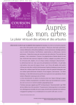
This article appeared in a journal published by Elsevier. The attached
copy is furnished to the author for internal non-commercial research
and education use, including for instruction at the authors institution
and sharing with colleagues.
Other uses, including reproduction and distribution, or selling or
licensing copies, or posting to personal, institutional or third party
websites are prohibited.
In most cases authors are permitted to post their version of the
article (e.g. in Word or Tex form) to their personal website or
institutional repository. Authors requiring further information
regarding Elsevier’s archiving and manuscript policies are
encouraged to visit:
http://www.elsevier.com/copyright
Author's personal copy
Biological Conservation 143 (2010) 2080–2091
Contents lists available at ScienceDirect
Biological Conservation
journal homepage: www.elsevier.com/locate/biocon
Woody species diversity in temperate Andean forests: The need for new
conservation strategies
Adison Altamirano a,*, Richard Field b, Luis Cayuela c, Paul Aplin b, Antonio Lara d, José María Rey-Benayas e
a
Departamento de Ciencias Forestales, Universidad de La Frontera, P.O. Box 54-D, Temuco, Chile
School of Geography, University of Nottingham, Nottingham NG7 2RD, United Kingdom
c
Departamento de Ecología, Centro Andaluz de Medio Ambiente, Universidad de Granada – Junta de Andalucía, Granada 18006, Spain
d
Instituto de Silvicultura, Universidad Austral de Chile, P.O. Box 567, Valdivia, Chile
e
Departamento de Ecología, Edificio de Ciencias, Universidad de Alcalá, 28871 Alcalá de Henares, Spain
b
a r t i c l e
i n f o
Article history:
Received 6 April 2009
Received in revised form 20 April 2010
Accepted 23 May 2010
Available online 16 June 2010
Keywords:
Biodiversity
Hotspot
Natural protected areas
Species richness
Spatial modelling
a b s t r a c t
Chile has more than half of the temperate forests in the southern hemisphere. These have been included
among the most threatened eco-regions in the world, because of the high degree of endemism and presence of monotypic genera. In this study, we develop empirical models to investigate present and future
spatial patterns of woody species richness in temperate forests in south-central Chile. Our aims are both
to increase understanding of species richness patterns in such forests and to develop recommendations
for forest conservation strategies. Our data were obtained at multiple spatial scales, including field sampling, climate, elevation and topography data, and land-cover and spectrally derived variables from satellite sensor imagery. Climatic and land-cover variables most effectively accounted for tree species richness
variability, while only weak relationships were found between explanatory variables and shrub species
richness. The best models were used to obtain prediction maps of tree species richness for 2050, using
data from the Hadley Centre’s HadCM3 model. Current protected areas are located far from the areas
of highest tree conservation value and our models suggest this trend will continue. We therefore suggest
that current conservation strategies are insufficient, a trend likely to be repeated across many other areas.
We propose the current network of protected areas should be increased, prioritizing sites of both current
and future importance to increase the effectiveness of the national protected areas system. In this way,
target sites for conservation can also be chosen to bring other benefits, such as improved water supply to
populated areas.
Ó 2010 Elsevier Ltd. All rights reserved.
1. Introduction
Loss of biodiversity is one of the most serious environmental
problems today because of the associated economic, scientific,
amenity and ecosystem service losses and the irreversible nature
of global extinction (Newton, 2007). Threats to biodiversity remain
strong, in large part because of continued increase in the rate of
human-mediated destruction and conversion of habitats (May
et al., 1995; Nagendra, 2001; Newton, 2007). The need to preserve
biodiversity is therefore urgent. One of the main actions to protect
biodiversity is to create or expand protected areas (Murphy, 1990;
Nagendra, 2001). Selection of areas for conservation should take
into consideration the representation and persistence of key attributes within sets of areas (Araújo, 1999). Species diversity is often
* Corresponding author. Tel.: +56 45 734159; fax: +56 45 325634.
E-mail addresses: [email protected] (A. Altamirano), [email protected] (R. Field), [email protected] (L. Cayuela), [email protected]
(P. Aplin), [email protected] (A. Lara), [email protected] (J.M. Rey-Benayas).
0006-3207/$ - see front matter Ó 2010 Elsevier Ltd. All rights reserved.
doi:10.1016/j.biocon.2010.05.016
used as a target attribute of biological communities to determine
areas of high conservation value (De Vries et al., 1999; Luoto
et al., 2002; Armenteras et al., 2006; Cayuela et al., 2006a);
although it is only one of the important variables, it often correlates with other key measures. In turn, species richness (by which
we mean the number of species in a given area), which is both the
simplest and most easily interpreted measure of species diversity,
tends to correlate strongly with the other measures (Whittaker
et al., 2001). Explaining patterns of species richness is, however,
a complex challenge because the diversity results from many interacting factors that operate at different spatial and temporal scales
(Diamond, 1988; Willis and Whittaker, 2002).
At fine scales, a variety of variables typically account for (or at
least correlate with) spatial diversity patterns (Whittaker et al.,
2001; Field et al., 2009). These fine-scale correlations are usually
weaker than those at broad scales (Field et al., 2009). Changes in
elevation, slope or exposure can determine the ecological response
of individual species and therefore contribute to overall changes in
species richness (Luoto et al., 2002). Human activities also influence the shape of geographical patterns of diversity in intensively
Author's personal copy
A. Altamirano et al. / Biological Conservation 143 (2010) 2080–2091
managed regions (Lawton et al., 1998; Ramírez-Marcial et al.,
2001; Cayuela et al., 2006b; Hall et al., 2009).
At broader spatial scales, patterns of species richness are correlated strongly with climatic variables (Currie, 1991; O’Brien, 1998;
O’Brien et al., 2000; González-Espinosa et al., 2004; Field et al.,
2005). If climate directly or indirectly determines patterns of richness, then when the climatic variables change, richness should
change in the manner that spatial correlations between richness
and climate would predict (Acevedo and Currie, 2003; Venevsky
and Veneskaia, 2003; Field et al., 2005). This might have important
consequences for long-term conservation, since prioritization of
highly diverse habitats today might not be effective in preserving
future hotspots of species richness in the face of climate change.
In this study, we develop empirical models to investigate present and future spatial patterns of woody species richness in temperate forests in south-central Chile. We follow the lead of
Cayuela et al. (2006a), who developed a predictive model using a
similar approach, which allowed identification of high-priority
areas for conservation of tropical forests in areas where the accessibility was limited. Our models include information obtained at
multiple spatial scales, including field sampling, climate, topography and land-cover variables. The applied goals of this research
are to inform attempts to prioritize the extant forest patches in
the region and to provide recommendations for their conservation.
This is of paramount importance as these forests are included in
the Global 200 initiative launched by the World Wildlife Fund
and the World Bank (Dinerstein et al., 1995), which focuses on
the most threatened eco-regions in the world. In addition, these
forests have been classified as one of the world’s biological hotspots, e.g. by Myers et al. (2000), because of their high degree of
endemism and presence of monotypic genera (Arroyo et al.,
1996; Smith-Ramírez, 2004). The temperate forests of Chile are
specifically considered to be vulnerable to impacts of climate
change (IPCC, 2001; Pezoa, 2003). Paradoxically, in Chile, at broad
scales the amount of land dedicated to conservation is inversely
correlated with the number of species and endemism (Armesto
et al., 1998). Thus, more than 90% of the 14 million hectares of protected land (CONAF et al., 1999) is concentrated in high latitudes
(>43°), leaving unprotected a large proportion of high-biodiversity
areas (Armesto et al., 1998). Here, we investigate whether the inverse relationship between amount of conserved land and numbers of species is true at a smaller spatial scale. For all these
reasons, establishing guidelines for prioritization of natural protected areas is a crucial step towards biodiversity conservation in
this important eco-region.
The specific objectives of this study are: (a) to assess the independent and joint contribution of different groups of variables in
describing the variation in woody species richness in the study
area, thereby increasing our knowledge and understanding of
Chile’s temperate Andean forests; (b) to develop a model to estimate present-day, fine-scale woody species richness across the
study area; (c) to develop a model to predict the effects of climate
change on woody species richness; and (d) to use the models to
evaluate the effectiveness of the currently protected areas for
maintaining biodiversity both now and in the face of climate
change. The models we develop can also be used to inform future
modification of the protected area network and to facilitate forest
restoration programmes.
2. Materials and methods
2.1. Study area
Our study was conducted in the Maule region of Chile, which
lies mainly in the Andean area between 35° and 36° latitude south
(Fig. 1). The study area covers approximately 270,000 ha and is be-
2081
tween 200 and 3900 m.a.s.l. The predominant soils are volcanic in
origin, with different degrees of development (Schlatter et al.,
1997). The predominant climate is of the Mediterranean type, with
annual precipitation averaging between 700 and 1300 mm and
concentrated mostly during the winter season, and an average annual temperature of 9 °C (Pezoa, 2003).
The area is characterized by the presence of secondary and oldgrowth forests (dominated by species like Nothofagus obliqua, Nothofagus glauca, Nothofagus dombeyi and sclerophyllous species over
2 m high and >50% coverage), shrublands (composed mainly of
low-height sclerophyllous species such as Criptocarya alba, Quillaja
saponaria and Lithraea caustica), exotic plantations (mainly of Pinus
radiata), agricultural lands, herbaceous vegetation, grasslands, and
other types of land-cover such as bare land, urban areas and water
bodies (Appendix A) (CONAF et al., 1999; Altamirano et al., 2007).
The intensification of land use, particularly firewood extraction
and selective logging, has caused much deforestation and forest
disturbance, which may have a negative impact on biodiversity
(Lara et al., 1996, 2003; Olivares, 1999; Echeverría et al., 2006).
The national protected areas system of Chile comprises 96 sites,
totalling approximately 14 million hectares and representing 19%
of the land (CONAF et al., 1999). The three main types of protected
area are National Parks, National Reserves and Natural Monuments. National Reserves are medium-sized areas that are protected with the aim of conserving species, soils and hydrological
resources; sustainable natural resource use is allowed. There are
two of these reserves in our study area: Altos de Lircay (approximately 12,000 ha) in the north, and Los Bellotos (approximately
400 ha) in the south (Fig. 1).
2.2. Field sampling and estimation of woody diversity
The study area was divided into approximately 700 cells, each
2 2 km. Of these, 82 were selected via a random sampling scheme
stratified by vegetation structure (see below), to contain field plots.
One field plot was located in each of these 82 cells so that it was as
close to the centre of the plot as possible, given the constraints that
it was within the most representative vegetation structure in terms
of percentage cover inside the cells, and was accessible. The plots
provided good coverage of the main vegetation and soil types, and
of the elevational range. In a pilot study, the numbers of species in
10 circular plots of 500 m2 and 250 m2 were compared. No significant differences were found (Student’s paired t-test, t = 2.3,
P = 0.16), so in order to allow greater replication, 250 m2 (i.e. 9 m radius) was set as the plot size. This also better matched the resolution
of the ASTER imagery used (see next section). The 82 plots were sampled in 2005 and 2006. In each, all trees and shrubs with a height
greater than 1.4 m were identified to species (see Appendix A),
counted and measured; from this, we calculated basal area. Fisher’s
alpha index, Shannon’s diversity index and species richness (number
of species observed) were calculated for each sample. Fisher’s alpha
and Shannon’s indices were, however, highly correlated with species
richness (r = 0.92, P < 0.0001; r = 0.87, P < 0.0001 respectively). Because of this strong similarity and the ease of interpretability, we
only report results for species richness.
2.3. Explanatory variables
To model species richness we focused on six climatic variables,
two topographic variables and three land-cover variables (Table 1).
We initially obtained 19 climatic variables from the WorldClim
database (www.worldclim.org). WorldClim is a set of global climate layers (climate grids) with a spatial resolution of 1 1 km
(Hijmans et al., 2005). This set includes 19 temperature, rainfall
and bioclimatic variables. The bioclimatic variables were derived
from the monthly temperature and rainfall values in order to be
Author's personal copy
2082
A. Altamirano et al. / Biological Conservation 143 (2010) 2080–2091
Fig. 1. Map of the study area in the Andean range.
more biologically meaningful, and represent annual trends in seasonality and extreme or limiting environmental factors (Hijmans
et al., 2005). We carefully examined the correlation matrix to
determine the degree of collinearity and redundancy between
these climatic variables (and the other explanatory variables), as
well as their correlations with species richness. We additionally
performed a hierarchical cluster analysis of these variables in order
to identify groupings of correlated explanatory variables. To
achieve this, we used the ‘Hmisc’ library (Harrell et al., 2009) of
the R environment (R Development Core Team, 2009), defining a
threshold of Spearman’s q = 0.6. We combined this information
with theoretical considerations to select climatic variables for further analysis that would minimise multicollinearity, while being
expected to account best for species richness, as recommended
by Carsten F. Dormann (pers. comm.). Multicollinearity tends both
to promote statistical artefacts (resulting in false model accuracy)
and to cause unstable parameter estimates, which are particular
problems when making predictions of future diversity. Thus we
chose the following climatic variables for the regression analyses
(Table 1): minimum temperature of the coldest month (Tmin), temperature seasonality (Tseas), mean annual precipitation (Pan), mean
precipitation of the driest month (Pmin) and precipitation seasonal-
Table 1
Climatic, topographic and land-cover variables used to model the spatial variation in woody species richness in the study area. Values given are for the 82 field plots.
(Code = abbreviation used, St. dev. = standard deviation, r (WSR) = Pearson’s correlation coefficient for the relationship with woody species richness, r (TSR) = correlation with tree
species richness, r (SSR) = correlation with shrub species richness, CV = coefficient of variation.)
Variable and unit of measurement
Code
Mean
St. dev.
Min.
Max.
r (WSR)
r (TSR)
r (SSR)
Response variables
Woody species richness
Tree species richness
Shrub species richness
n.a.
n.a.
n.a.
8.3
5.0
3.3
3.1
2.4
1.7
2
0
0
16
11
8
n.a.
0.83***
0.63***
0.83***
n.a.
0.10 n.s.
0.63***
0.10 n.s.
n.a.
Climatic variables
Elevation (m) – untransformed
Minimum temperature of coldest month (°C)
Temperature seasonality (st. dev.)
Annual precipitation (mm)
Precipitation of driest month (mm)
Precipitation seasonality (CV 100)
ELEV
Tmin
Tseas
Pan
Pmin
Pseas
674
0.31
4.54
1080
15.8
83.9
292
1.29
0.09
76
1.6
1.9
288
3.0
4.39
853
11
78
1603
2.2
4.74
1260
18
88
0.50***
0.50***
0.28*
0.22*
0.47***
0.33**
0.63***
0.60***
0.42***
0.40***
0.53***
0.44***
0.03 n.s.
0.05 n.s.
0.09 n.s.
0.16 n.s.
0.11 n.s.
0.02 n.s.
Topographic variables
Aspect (degrees from north)
Slope (degrees)
ASPE
SLOP
83.2
14.2
55.7
8.5
1
1
180
38
0.02 n.s.
0.18 n.s.
0.17 n.s.
0.11 n.s.
Land-cover variables
Normalised difference vegetation index
Normalised difference infrared index
Vegetation structurea
NDVI
NDII
VST
0.678
0.719
n.a
0.196
0.064
n.a.
0.056
0.455
1
1.000
0.825
4
0.13 n.s.
0.23*
n.a.
0.01 n.s.
0.11 n.s.
n.a.
n.a. = correlation is not applicable.
n.s. = not significant.
Categorical data: four categories (1 = open shrubland, 2 = dense shrubland, 3 = arborescent shrubland, 4 = forest).
*
P < 0.05.
**
P < 0.01.
***
P < 0.001.
a
0.21 n.s.
0.17 n.s.
0.26*
0.26*
n.a.
Author's personal copy
A. Altamirano et al. / Biological Conservation 143 (2010) 2080–2091
ity (Pseas). Mean annual temperature was strongly correlated with
Tmin (r = 0.98); we chose Tmin because it is very similar to minimum
monthly potential evapotranspiration calculated by the Thornthwaite method, which previous empirical and theoretical work
has shown to be a good predictor of woody species richness (e.g.
Field et al., 2005). In our dataset, Tmin correlated more strongly
with species richness than Tmean, supporting our reasoning. Pmin
is appropriate in climates where precipitation is lowest during
the summer months, as in our study area, because it represents a
strong constraint on growth.
Elevation was derived from a digital elevation model, with a
spatial resolution of 90 90 m, based on the Shuttle Radar Topography Mission (SRTM). The SRTM data are available from the Global Land Cover Facility (GLCF) website (http://www.landcover.org).
It was classed as a climate proxy for several reasons. Elevation is a
powerful and very precise determinant of small-scale climatic variation, particularly temperature; this is because of the close association between temperature and elevation that results from the
effects of the adiabatic lapse rate. The relationship between elevation and precipitation is less strong, more indirect and more complex. In this study, elevation, with its resolution of 90 90 m, is
much more precisely measured than the WorldClim variables (resolution 1 1 km), so it can be expected to model climate (particularly temperature) well for the field plots. Given the scale of the
field plots and the nature of the study area, elevation was also a
poor topographic measure, indicating nothing about topographic
heterogeneity, nor about aspect. This reasoning is backed up by
the fact that, in our dataset, elevation was not correlated with
topographic variables (r = 0.035 and 0.044 for slope and aspect
respectively), but was almost perfectly inversely correlated with
Tmin and mean annual temperature (r = 0.95 and 0.94) despite
the difference in resolution. The correlation between elevation
and precipitation was moderate (r = 0.55 for Pan; r = 0.71 between 1/elevation and Pmin).
The topographic variables used were aspect and slope (Table 1).
Aspect was measured as degrees from north. These variables were
derived from the digital elevation model.
We performed image analysis on remotely sensed imagery, acquired in March 2003 by the Advanced Spaceborne Thermal Emission and Reflection Radiometer (ASTER), to identify different forest
types in relation to their degree of disturbance and to calculate different vegetation indices. We georeferenced the image using 43
control points derived from vector maps of roads and rivers, obtained from the Native Vegetation Survey (CONAF et al., 1999),
resulting in an estimated error of less than one pixel. We atmospherically corrected the image using the dark pixel subtraction
method and features such as water bodies (Mather, 1999).
We performed a supervised land-cover classification (Aplin,
2004) of the image using the maximum likelihood algorithm (Lillesand et al., 2004). Four different types of vegetation structure (VST)
were identified in relation to human disturbance: open shrubland
(VST1), dense shrubland (VST2), arborescent shrubland (VST3) and
forest (VST4), which includes old-growth forest, secondary forest
and an intermediate condition (Altamirano and Lara, 2010). Other
land-cover types were excluded from the analyses and predictions
reported herein. Training sites were selected using different
sources of information such as vegetation maps, aerial photographs from 2003 and field visits conducted between 2004 and
2006. The overall accuracy of the supervised classification was
92%. The lowest accuracy was obtained for shrubland and secondary forests; this was because of spectral confusion between these
two classes. The pre-processing and classification of remotely
sensed data were performed using the ERDAS Imagine 8.4Ò software (ERDAS, 1999).
In addition, we calculated two spectral indices: the normalised
difference vegetation index (NDVI) and the normalised difference
2083
infrared index (NDII). The NDVI was calculated as the difference
between the near-infrared and red reflectances divided by their
sum, which represents a measure of vegetation productivity (Turner et al., 2003; Aplin, 2005). The NDII was calculated as the difference between the near-infrared and mid-infrared reflectances
divided by their sum, which is related to the hydric stress (Bannari
et al., 1995; Gao, 1996). We did not use spectral bands from the ASTER image because they were both highly correlated with, and less
interpretable than, NDVI and NDII (|r| > 0.85, P < 0.001).
2.4. Statistical analyses
To inform subsequent analysis, we used variance partitioning to
explore the independent and joint contribution of all available
explanatory variables, including all 19 WorldClim variables and
elevation (‘climatic’ category), the spectral bands from the ASTER
image and derived land-cover variables (‘land-cover’) and slope
and aspect (‘topographic’) in accounting for spatial variation in
woody species richness. The partition of the variance is derived
from partial redundancy analyses (RDA) and was used to determine the proportions that could be attributed to the single and
combined effects of explanatory variables (Legendre and Legendre,
1998), using adjusted R2 ratios (Peres-Neto et al., 2006). These
analyses were computed using the ‘vegan’ library (Oksanen et al.,
2008) of the R environment (R Development Core Team, 2009).
The results of the variance partitioning informed the selection
of variables for modelling, in which we used multiple regression
to develop models to predict woody species richness in the study
area. Most regression analysis was performed with the S-PLUS
6.0 software (Insightful Corporation, 2001); spatial analysis was
conducted using SAM (Rangel et al., 2006). Before performing multiple regression, we examined the correlation matrix and the hierarchical cluster analysis. We noted explanatory variables that were
highly correlated (|r| > 0.6) and the clusters of such correlated variables, which might therefore lead to problems associated with
multicollinearity. We used the same mix of theoretical and statistical considerations as described above for selection of WorldClim
variables, to determine which of all the explanatory variables could
be combined in any one model. We also calculated the variance
inflation factor (VIF) for all terms in all multiple-regression models,
to quantify any remaining multicollinearity, using a maximum
allowable level of VIF of 4. In addition, we examined the correlations between species richness and all selected explanatory variables (Table 1). Further, because relationships between species
richness and environmental variables are often curvilinear (Austin,
1980) and interactive (Francis and Currie, 2003), we included quadratic and cubic terms in the models, as well as some interactions
expected from previous research (e.g. between temperature and
water variables).
Our modelling procedure was step-wise and manual (Murtaugh, 2009), using a combination of model building and model
simplification. We produced the first model by building from the
null model (the mean), adding terms in order of explanatory
power, defined as the change in residual sum of squares resulting
from the addition of individual terms to the current model. Model
building finished when no more terms were both significant and
reduced AIC (Akaike Information Criterion) (Venables and Ripley,
2002; Anderson and Burnham, 1999). We then used a similar procedure, but with different starting variables (chosen according to
variable type and variance accounted for) and different orders of
addition. We also produced a series of models by simplifying from
various maximal models (Crawley, 2002). It was necessary to simplify from more than one maximal model because the sample size
of 82 did not support highly complex models. We compared all
models obtained statistically using P-values, AIC and the proportion of variation accounted for (R2). We also used ‘Model Selection
Author's personal copy
2084
A. Altamirano et al. / Biological Conservation 143 (2010) 2080–2091
and Multi-model Inference’ in SAM to rank over 16,000 possible
models by AICc and AIC-weights and to calculate the ‘importance’
of each variable across all the models. This combination of model
fitting approaches allowed confidence in the robustness of the results. Selection of the ‘best’ models was based on both theoretical
criteria (plausibility, generality, simplicity, parsimony) and statistical strength (O’Brien et al., 2000).
We used Moran’s I to evaluate the spatial autocorrelation of the
residuals of the fitted models. Finding no residual spatial autocorrelation means that we can assume the significance values to be
reliable, and that we do not need to introduce the further uncertainties (coefficient instability) associated with spatial regression
(Bini et al., 2009). We checked the model residuals for normality
using histograms and the Kolmogorov–Smirnov test. We assessed
homoscedasticity via residual plots, and we mapped model residuals to examine their spatial patterning. To validate the predictive
power of the models, we used a bootstrap approach for each model. This method generates new samples with replacement from the
original sample, allowing a quantification of the error introduced
by data uncertainty as well as model estimation procedure (Quinn
and Keough, 2003).
We used the resulting regression models to predict current species richness values for parts of the study area where there were no
field plots. This was done for every pixel in the ASTER imagery and
involved using the coefficients from the models and substituting
the applicable values for the explanatory variables, to calculate
predicted current species richness.
2.5. Climate-change scenario
We used the coefficients derived from modelling current woody
species richness to predict future species richness across the study
area, using climatic data obtained for a climate-change scenario.
Climate scenarios are guesses of future climates, based on assumptions about future emissions of greenhouse gases and other pollutants, and obtained via general circulation models, such as CCCMA,
HadCM3 and CSIRO. We used projected climate data for 2050, from
the Hadley Centre’s climate model (HadCM3 Worldclim implementation) under the low (B2a) CO2 emissions scenario (Zhang
and Nearing, 2005), obtained from WorldClim. We used scenario
B2a because it emphasizes more regionalized solutions to economic, social, and environmental sustainability (Zhang and Nearing, 2005).
2.6. Conservation value
To analyse conservation value we produced maps categorizing
the predicted current woody species richness into three levels:
high (>8 species), medium (5–8 species) and low (<5 species).
When examining tree species richness, we used >6, 4–6 and <4
species respectively. This was done for all pixels of the ASTER image (with a spatial resolution of 15 m) that had land-cover in one of
the categories VST1, VST2, VST3 and VST4. Pixels classified as other
categories were excluded from further consideration. Predicted future species richness was categorized using the same criteria and
results were compared in terms of: (1) forest area occupied by each
conservation value category now and in 2050; (2) overall forest
area that will change to a different conservation value category
by 2050; and (3) forest area in current natural protected areas assigned to different conservation value categories now and in 2050.
3. Results
We recorded 67 woody species (28 trees and 39 shrubs) in the
field plots (Appendix A), with a mean (±SD) number of species per
plot of 8.3 (±3.1), ranging from 2 to 16. We found significantly lower mean tree and overall (tree + shrub) species richness in VST1
(open shrubland) than in the other three categories (ANOVA,
P = 0.006 and 0.017 respectively), but no differences between
VST2 (dense shrubland), VST3 (arborescent shrubland) and VST4
(forest). Therefore for regression modelling we re-categorized the
forest structure variable into two categories: VST1 and closed canopy (VST2, VST3 and VST4 combined) because this is more robust
and parsimonious (Crawley, 2002). Interestingly, there was no significant difference between VST categories in either tree or shrub
abundance.
The strongest single-variable correlates of both tree and overall
species richness in the 82 field plots were Tmin, Pmin and ELEV (Table 1). None of the explanatory variables in Table 1 correlated with
shrub species richness at the 1% significance level. At the 5% level
only NDVI and NDII were significant, both correlating weakly and
negatively with shrub species richness (Table 1); this effect was
driven by the open shrubland (r = 0.50 for both NDVI and NDII)
and was not significant for the denser woody vegetation categories.
The difference in shrub diversity between the different VST categories was also not significant. Basal area of woody plants correlated
negatively with shrub species richness (r = 0.31, P = 0.005) and
band 5 of the ASTER image correlated positively (r = 0.36,
P = 0.0009). Band 5 and basal area represented the strongest statistical model, with neither NDVI nor NDII significantly improving it,
but this model only accounted for 18% of the variation, had nonnormal residuals and contained potential circularity. Overall, then,
we were unable to produce a satisfactory model of shrub species
richness, which also did not correlate significantly with tree species richness (Table 1). Models of overall woody species richness
were all qualitatively identical to, but quantitatively weaker than,
those for tree species richness; they were driven by the tree species
richness pattern, with shrub species richness effectively adding
noise. We therefore focus on reporting the results for tree species
richness.
Minimum temperature (Tmin) correlated positively and ELEV
negatively with tree species richness, both consistent with greater
energy allowing more species. The correlation between tree species richness and Pmin, however, was negative, both singly and
when included in multiple-regression models. Both log and inverse
transformations of ELEV improved the linearity of its association
with tree species richness, 1/ELEV the more so, which also improved the normality of regression residuals compared with models using ln(ELEV). Using 1/ELEV made the relationship with tree
species richness positive and increased the strength of the bivariate correlation to r = 0.66.
In variance partitioning, topographic, climatic, and land-cover
variables accounted for 2%, 52% and 7%, respectively, of the adjusted variance of woody species richness (Fig. 2). Overlap between
the categories in variance accounted for was minimal (Fig. 2), supporting our contention that elevation acts as a climatic, not topographic, variable in our dataset.
3.1. Predictive models of species richness
Tmin correlated strongly with 1/ELEV (r = 0.91), so only one of
the two variables could be used in the same regression model.
We developed models independently using both variables. In all
cases, as with simple correlation, 1/ELEV gave a closer fit with woody species richness (Model 1, Table 2a). However, for predicting
species richness for the year 2050 we preferred models featuring
Tmin instead of 1/ELEV (Models 2a and b). Temperature has a direct
physiological effect on species performance, while elevation is a
surrogate variable for a mixture of influences, but driven by temperature (Guisan and Zimmermann, 2000; Pausas and Austin,
2001), so temperature is preferred on theoretical grounds. Most
Author's personal copy
2085
A. Altamirano et al. / Biological Conservation 143 (2010) 2080–2091
Fig. 2. Venn diagram of the partition of the variation of tree species richness for
climatic, topographic and land-cover variables. Table 1 shows which of the key
variables were included in each category; other WorldClim data were included as
‘climatic’ and other variables derived from ASTER imagery were included as ‘landcover’. The rectangle represents the total variance of tree species richness while
each circle represents a given group of explanatory variables. The adjusted R2
(expressed as % of the variance in tree species richness) is presented for each part of
the Venn diagram; if missing this fraction does not differ significantly from 0.
Intersections between circles represent the fraction of the variance of tree species
richness jointly accounted for.
of the effect of elevation is related to temperature and precipitation, and with climatic changes over the next 40 years, the regression coefficients derived from current conditions for elevation are
not applicable to prediction for 2050. Therefore for prediction of
future species richness, and for comparison of the conservation value of protected areas now and in the future, we used the best
models that were based on Tmin (Models 2a and 2b; Table 2b and
c). VST was considered appropriate for 2050 because its main
determinant is human activity (disturbance); its inclusion in Models 2a and b assumes no change in the disturbance regime during
the first half of the 21st century.
The ‘best’ regression models (Models 1 and 2a,b) were selected
on the grounds of theoretical plausibility, simplicity and statistical
strength (secondary to the other two). These best models included
two alternative models based on Tmin: Models 2a and 2b (Table 2).
These were statistically indistinguishable and both were ecologically plausible. The strongest effects are the same in both models,
and in a reduced model with only VST and Tmin. The first is a strong
increase in tree species richness with increased Tmin, of approximately 1 species per 1 °C. The second is approximately 1.5 fewer
species in open shrubland than the other vegetation types. Thus
the core of the models is the same; they differ in the final variable
included, which in each case only accounts for an additional 4% of
the variance (approximately). In Model 2a, this is Tseas, with a decrease of approximately 6 tree species for every 1 °C increase in
seasonality (measured as the standard deviation; Table 1); this is
ecologically plausible (Jocqué et al., 2010). In Model 2b, the third
variable is Pmin, with a decrease of approximately 1 tree species
for every 3 mm increase in driest-month precipitation. Exploring
this negative effect further (see also Table 1), we found a negative
correlation (r = 0.40) between Pmin and overall tree abundance,
suggesting a competition or crowding effect, coupled with a more
individuals effect (positive correlation, r = 0.54, between tree abundance and tree species richness). However, using data for basal
area and average tree diameter for all plots in the dataset, we
found no correlation between either variable and Pmin. Nor did
either basal area or average tree diameter correlate with tree species richness. So, while Pmin could be measuring a competition effect, we are far from certain that it does indeed do so, or
whether it is measuring another biologically meaningful effect
such as inhibition of seed germination or seedling survival (Donoso, 1994), or whether the apparent effect is due to correlation with
other important biological influences. Because Pmin and Tseas are
positively correlated (r = 0.58) and neither is even close to significant when the other is in the model, Models 2a and 2b are straight
alternatives and we are unable satisfactorily to reject one in favour
of the other. Therefore our predictive modelling was based on average predictions from the two models, hereafter referred to collectively as Model 2. This averaging of predictions, a form of
ensemble forecasting (Araújo and New, 2007), should also increase
the robustness of the predictions.
All models presented in Table 2 are statistically significant
(P < 0.0001) and all rely on few explanatory variables, reducing
the likelihood of artefact, which is particularly important when
predicting future species richness. All the models met assumptions
of homoscedasticity and normality of residuals. For all the models,
Moran’s I values for residuals were not significant for any of the
short distance classes (Fig. 3), indicating no inflation of degrees
of freedom resulting from spatial autocorrelation, and the absence
Table 2
‘Best’ models for predicting spatial variation in tree species richness in the study area: (a) Model 1 – model for predicting current species richness (best model using all available
variables); (b) Model 2a – model for predicting future species richness and for comparison of predictions; (c) Model 2b – alternative model for predicting future species richness
and for comparison of predictions. D.f. = degrees of freedom; VIF = variance inflation factor; R2 = proportion of the variance accounted for (tested by deletion from the model);
AIC = Akaike Information Criterion; root mean square error (RMSE) = square root of the error variance. All predictions are for plots of 250 m2. See Table 1 for full variable names
and units.
Model
Coefficient
Null model
D.f.
VIF
t-value
p
R2
81
(a) Model 1 (RMSE: 3.0)
Intercept
1/ELEV(in km)
VST
Overall model
0.34
2.35
1.59
(b) Model 2a (RMSE: 3.3)
Intercept
VST
Tmin
Tseas
Overall model
30.18
1.54
0.93
5.88
(c) Model 2b (RMSE: 3.3)
Intercept
VST
Tmin
Pmin
Overall model
9.51
1.51
0.81
0.38
AIC
383.5
1
1
2
1.00
1.00
0.53
8.07
3.33
0.597
0.000
0.001
0.000
0.41
0.07
0.50
376.7
338.2
329.6
1
1
1
3
1.01
1.21
1.20
2.79
3.09
5.40
2.47
0.007
0.003
0.000
0.017
0.000
0.07
0.20
0.04
0.47
344.5
361.0
341.2
337.3
1
1
1
3
1.01
1.66
1.65
2.90
3.02
3.98
2.31
0.005
0.003
0.000
0.024
0.000
0.06
0.11
0.04
0.46
344.8
350.9
341.2
338.0
Author's personal copy
2086
A. Altamirano et al. / Biological Conservation 143 (2010) 2080–2091
of intrinsic autocorrelation that could disturb the Type I error rates
and the coefficient estimates. In other words, the regression models have accounted for the spatial autocorrelation present in the
species richness data. This also means that our predictive model
is of the type considered the best for predicting responses to climate change by Algar et al. (2009): they concluded that the most
accurate predictions of shifts in species diversity in response to climate change are obtained via the single best richness–environment regression model, after accounting for the effects of spatial
autocorrelation. Further, our model has the advantage that the spatial autocorrelation is accounted for via ordinary least-squares
regression, so that there is no chance of real effects being ‘corrected
for’ while removing spatial autocorrelation in spatial regressions.
3.2. Predicted species richness
Present-day woody species richness was predicted for the
whole study area using Model 1 (Fig. 4a) and Model 2 (Fig. 4b).
Model 2 predicted slightly higher species richness on average than
Model 1, but the spatial patterns were very similar. The areas of
higher predicted richness at this scale (250 m2) are concentrated
mainly in the western locations of the study area and in valleys,
at lower elevation and higher temperatures. These areas are dominated by shrubland and arborescent vegetation. The two protected
areas in the study area have relatively low levels of predicted current species richness (Fig. 4a and b).
Our predictions for 2050 (Fig. 5a) suggest that the higher
ground in the east of the study area will increase in tree species
richness, while the lower ground in the west will decrease. Thus
the species-richness gradient across the study area is expected to
persist but weaken (compare Fig. 5a with Fig. 4b) with climate
change. Overall, of the 1296 km2 for which we made predictions,
a net loss of species was predicted for 490 km2 (38%) and a net
gain for 698 km2 (54%), the remainder staying approximately constant. Using our categories for conservation value, 58% of the pixels (each 225 m2) were predicted by Model 2 to have present-day
woody species richness in the low category (0–3 species), with
31% having more than 6 species (Fig. 6a). Of all the pixels, 34%
were predicted to change from low to medium conservation value, while 16% were predicted to change from high to medium
(Fig. 6a).
Only 29.0 km2 of the land currently designated as protected
areas is covered by woody vegetation, as judged by our analysis
of the ASTER image. All of this area is currently in the low conservation priority (value) category, according to Model 2. Our map
predictions suggest that 8.6 km2 (30%) of the protected area will
improve to the medium category by 2050, the rest remaining
‘low’ (Fig. 6b).
4. Discussion
Fig. 3. Correlograms for tree species richness, fitted values and residuals of the
‘best’ regression models: (a) Model 1, (b) Model 2a, (c) Model 2b. Equal distance
classes; only classes with n > 100 shown. See Table 2 for model specifications
(n = 82 cells).
We found that the highest tree species richness occurs in low
and medium elevation areas, with the highest minimum temperatures, and where there is relatively dense woody vegetation cover.
The protected areas within the study area contain very low tree
species richness and our modelling suggests that the areas of highest tree conservation value are far from the currently protected
areas. Our predictions for changed climate indicate reduced tree
diversity where it is currently high and increased diversity where
it is currently low. The currently protected areas may therefore
slightly increase in tree conservation value over the next 40 years,
but will still be relatively low in diversity. Meanwhile, the areas of
greatest species richness are predicted to suffer losses, thereby
degrading in conservation value. The resulting predominance of
areas of relatively average conservation value suggests a need for
the conservation of greater areas of forest. Greater connectivity
of patches of woody vegetation may also be important. Although
the protected areas may be important for species other than woody
plants, their continued low value for tree species conservation is of
great conservation concern because Chile has more than half of the
temperate forests in the southern hemisphere (Donoso, 1994), because of the uniqueness of these forests (Smith-Ramírez, 2004),
and because of the high levels of threat to these forests (Dinerstein
et al., 1995).
These concerns about tree conservation that arise from our species richness modelling are backed up by our field observations of
threatened species within our study plots. We recorded 4 threatened species, all of which are trees: Nothofagus glauca, Austrocedrus chilensis, Beilschmiedia berteroana and Cytronella mucronata.
These species have a restricted distribution and highly specific
habitats (Hechenleitner et al., 2005). Migration capabilities for
these species under climate change may well be limited. N. glauca
(by far the most common of the four in our field plots) is restricted
largely to the Maule region and is found mainly in intermediate
elevation sites (Hechenleitner et al., 2005), so may not be much affected by climate change. However, B. berteroana may be negatively affected by climate change because its habitat is coincident
with sites where species richness is expected to decrease. To aggra-
Author's personal copy
A. Altamirano et al. / Biological Conservation 143 (2010) 2080–2091
2087
Fig. 4. Map of predicted current woody species richness in 225 m2 pixels. (A) Current tree species richness according to Model 1; (B) current tree species richness according to
Model 2 (average of predictions from Models 2a and 2b); (C) current conservation priority (value) category, as defined by tree species richness predicted by Model 2 (low = <4,
medium = 4–6, high = >6). No colour means no prediction because the pixel is not currently classed as any of the land-cover types in our analyses. See Table 2 for model
specifications.
vate the problem, only 8 sub-populations of this species have been
identified in the country (Hechenleitner et al., 2005). The other two
threatened species have wider distributions and may therefore be
less vulnerable to climate change. An additional consideration is
that many mountain plants reproduce vegetatively and grow
slowly; consequently they are likely to take a long time to disperse
into new, climatically suitable areas (Trivedi et al., 2008).
There are continuing threats to temperate Andean forests and
their biodiversity, such as hydroelectric-power projects and the rapid growth of the exotic plantations industry (Lara et al., 2003). In
recent years, exotic plantations have expanded specifically in the
south-central temperate forests of Chile (Echeverría et al., 2006)
because of the growth of the pulp and wood industry (Lara et al.,
2003). These developments may facilitate the establishment and
Author's personal copy
2088
A. Altamirano et al. / Biological Conservation 143 (2010) 2080–2091
Fig. 5. Map of predicted tree species richness in 2050, in 225 m2 pixels. (A) Tree species richness in 2050 according to Model 2 (average of predictions from Models 2a and
2b); (B) change in tree species richness from now to 2050, according to Model 2; (C) uncertainty for 2050 tree species richness predictions (absolute difference between the
predictions of Models 2a and 2b); (D) conservation priority (value) category in 2050, as defined by species richness predicted by Model 2 (low = <4, medium = 4–6, high = >6).
No colour means no prediction because the pixel is not currently classed as any of the land-cover types in our analyses. See Table 2 for model specifications.
Fig. 6. Current forest area by conservation priority (value) category (horizontal axis
labels), and how these conservation priorities will change in the year 2050
(shading), according to Model 2 (average of predictions from Models 2a and 2b). (A)
In the study area and (B) in the current protected areas. See Table 2 for model
specifications.
invasion of alien species, which may also be enhanced by predicted
rises in the frequency of natural disturbances (e.g. forest fires), and
ultimately reduce the cover of native vegetation (Pickering et al.,
2008). Studies in Chile have shown that alien species are moving
into native forests in national parks in mountain areas (Pauchard
and Alaback, 2004). Given these various forms of disturbance in
the study area, our results suggest that protected areas are
important for conservation: we found that the most disturbed
areas of woody vegetation have the lowest tree species richness,
with no accompanying increase in shrub species richness. This suggests that one way of improving conservation is to minimize
disturbance.
Our predictions, by necessity, assumed no change in protection/
disturbance regime (land-cover type). Nonetheless, our coefficients
for the disturbance variable (VST) can be used to explore future
scenarios in which disturbance regimes do change in prescribed
ways. Our assumption of no increase in disturbance may be optimistic, unless the protected area network is modified, or unless
parts of the landscape not in protected areas are managed for woody plant conservation. We consider that both strategies should be
implemented. New protected areas should be created, and because
our prediction maps indicate that current high-priority sites are
coincident with high-priority sites in 2050, we suggest that sites
that have high tree species richness now should be targeted for national protection. In the study area, these sites include river valleys,
and so this should help to ensure reliable supplies of clean water
downstream. Such targeting is important: Babcock et al. (1997)
demonstrated that enrolling land into a conservation programme
on the basis of the lowest cost of purchasing land (as has been
the case for many of Chile’s protected areas) is a far less efficient
use of taxpayers’ money than targeting land on the basis of the
cost–benefit ratio of that land. The application of newer approaches to protected area design could help stakeholders find designs that simultaneously maximize ecological, societal and
industrial goals (Gonzales et al., 2003). Planning tools such as Sites
Author's personal copy
2089
A. Altamirano et al. / Biological Conservation 143 (2010) 2080–2091
(Davis et al., 1999) and Marxan (Game and Grantham, 2008) represent good examples. Of high relevance to areas not formally protected, in 2008 Chile passed a new law that supports native
forest management and biodiversity conservation. This law gives
economic incentives to landowners to engage in biodiversity conservation. Again, the law can target high-priority conservation
sites, as indicated by our prediction maps, for improved effectiveness (Macmillan et al., 1998). Subsidies to encourage landowners
to manage their land in ways that increase the provision of nonmarket benefits may also be appropriate (Van der Horst, 2007).
Our research represents a starting-point, but more work is
needed to inform conservation in the temperate Andean forests.
First, our model should be seen as a tool, for addressing urgent conservation issues, that should be assessed, discussed and evaluated
further. Also, we have not investigated individual species’ requirements; for example, species-specific conservation measures for endemic and threatened species, including ex situ conservation, may
be required. Woody species may have differential abilities to cope
with climate change (Parolo and Rossi, 2008), and habitat connectivity may be important in enabling some to migrate. Species usually differ in their habitat requirements and habitat mosaics may
be appropriate in meeting each species’ needs (Drechsler et al.,
2007). In this context, important future challenges for biodiversity
conservation research are to investigate beta diversity and determine how much habitat heterogeneity is needed to maintain species diversity at coarser scales than in our study. Furthermore, we
used climatic and topographic data that are widely used for this
sort of analysis (WorldClim and SRTM). However, some environmental data sets may be less useful in some areas (i.e. rugged, remote and steep terrain) and scales (Peterson and Nakzawa, 2008).
Therefore, further corroboration and testing of other source information will be necessary.
Our study adds to knowledge and understanding of species
richness patterns and their correlates. Tree species richness correlated most strongly with temperature-related variables (elevation
and minimum temperature), which is common at broad scales
but less common at the finer scale of our study (Field et al.,
2009). This may be because we sampled quite a large altitudinal
range, and fits with the findings of Bhattarai and Vetaas (2003).
The closer match, in terms of scale of measurement, between elevation and species richness, compared with climatic variables,
probably explains the stronger correlation of species richness with
elevation. The relatively small amount of variation accounted for
by Pmin and Tseas is probably due, in large part, to the fact that both
vary little in the data for our study plots (Table 1). Despite their
coarse scale of measurement, climatic variables performed well
in accounting for tree species richness patterns, relative to the
fine-resolution variables such as slope, aspect and NDVI. This supports the contention (Cayuela et al., 2006a) that broad-scale patterns (e.g. Hawkins et al., 2003; Field et al., 2005) can be
replicated across altitudinal gradients at finer spatial scales. In
addition, there was a positive correlation (r = 0.54) between tree
abundance and tree species richness in our field plots; adding tree
abundance to any of the final tree species richness models led to
about a 5% increase in variation accounted for. This suggests a
‘more individuals’ effect, whereby more individuals tend to be
associated with more species (Srivastava and Lawton, 1998; Currie
et al., 2004). However, this was of little use for modelling because
our best model of tree abundance contained only Tmin and only accounted for 26% of the variation.
Our best tree species richness model accounts for approximately 50% of the variance, which is quite typical for this scale
(Field et al., 2009). Small-grain species richness is hard to predict,
as it depends on so many interacting factors and chance events
(Diamond, 1988; Whittaker et al., 2001; Willis and Whittaker,
2002), and small-grained studies typically account for less than
50% of the variation in species richness, even at geographic extents
spanning hundreds of kilometers (Field et al., 2009). Not surprisingly, therefore, even our best models left much of the variation
unaccounted for, suggesting that other, unmeasured factors also
influence woody species richness in the study area. Hydrological,
soil factors and biotic interactions might account for some of the
residual variation. This is particularly relevant to shrub species
richness, which did not correlate strongly with any of our measured variables, and which we could not model well enough to allow prediction. The strongest correlation with shrub species
richness was a negative one with basal area, suggesting that shading by trees may reduce shrub diversity. This accords with the recent findings by Oberle et al. (2009) that understorey plant species
richness in field plots of similar size to ours correlates much less
with regional productivity-related variables than does tree species
richness, and that canopy density partly controls shrub species
richness at this scale.
Overall, our research contributes to understanding of globally
important temperate Andean forests, and represents a step towards targeting conservation of the forests more effectively.
Acknowledgments
This research was made possible by funding from MECESUP
project AUS 0103; BIOCORES (Biodiversity conservation, restoration, and sustainable use in fragmented forest landscapes) project
ICA-CT-2001-10095; and the FORECOS Scientific Nucleus P04065-F (MIDEPLAN). We are grateful to Andrés Rivera from Centro
de Estudios Científicos (CECS) for the acquisition of the ASTER image needed to develop the research. Thanks to Raúl Bertín and
Renato Rivera for assistance with the field work, and Jonathan Barichivich for species identification, all from Universidad Austral of
Chile.
Appendix A
List of tree species and shrubs sampled in the study area.
Nomenclature follows the Index Kewensis, except for those cases
in which no record was found, for which the Gray Herbarium Card
Index (http://www.ipni.org) was used.
Species
Family
Trees
Acacia caven (Molina) Molina
Aextoxicon punctatum Ruiz & Pav.
Austrocedrus chilensis (D. Don) Pic.Serm. &
M.P.Bizzarri
Beilschmiedia berteroana (Gay) Kosterm.
Crinodendron patagua Molina
Cryptocarya alba (Molina) Looser
Citronella mucronata (Ruiz & Pav.) D.Don
Dasyphyllum diacanthoides (Less.) Cabrera
Drimys winteri J.R. Forst. & G. Forst.
Embothrium coccineum J.R. Forst. & G. Forst.
Gevuina avellana Molina
Kageneckia oblonga Ruiz & Pav.
Laureliopsis philippiana (Looser) Schodde
Laurelia sempervirens (Ruiz & Pav.) Tul.
Lithraea caustica Hook. & Arn.
Lomatia dentata R. Br.
Lomatia hirsuta (Lam.) Diels
Luma apiculata (DC.) Burret
Luma chequen F. Phil.
Leguminosae
Aextoxicaceae
Cupressaceae
Lauraceae
Elaeocarpaceae
Lauraceae
Icacinaceae
Asteraceae
Winteraceae
Proteaceae
Proteaceae
Rosaceae
Monimiaceae
Monimiaceae
Anacardiaceae
Proteaceae
Proteaceae
Myrtaceae
Myrtaceae
(continued on next page)
Author's personal copy
2090
A. Altamirano et al. / Biological Conservation 143 (2010) 2080–2091
Appendix A (continued)
Species
Family
Maytenus boaria Molina
Nothofagus alpina (Poepp. & Endl.) Oerst.
Nothofagus dombeyi (Mirb.) Oerst.
Nothofagus glauca (R. Phil) Krasser
Nothofagus obliqua (Mirb.) Oerst.
Nothofagus pumilio (Poepp. & Endl.) Krasser
Persea lingue (Miers ex Bertero) Nees
Peumus boldus Molina
Quillaja saponaria Molina
Celastraceae
Fagaceae
Fagaceae
Fagaceae
Fagaceae
Fagaceae
Lauraceae
Monimiaceae
Rosaceae
Shrubs
Acrisione denticulata (Hook. & Arn.) B. Nord.
Aristotelia chilensis Stuntz
Azara celastrina D. Don
Azara dentata Ruiz & Pav.
Azara petiolaris (D. Don) I.M.Johnst.
Azara serrata Ruiz & Pav.
Baccharis concava Pers.
Baccharis linearis (Ruiz & Pav.) Pers.
Baccharis salicifolia (Ruiz & Pav.) Pers.
Berberis chilensis Gill.
Berberis grevilleana Gill.
Berberis microphylla G. Forst.
Buddleja globosa C. Hope
Cestrum parqui L’Hér.
Colletia spinosissima J.F. Gmel.
Collihuaja sp 1
Discaria chacaye (G. Don) Tortosa
Ephedra chilensis C. Presl
Undetermined sp1
Fabiana imbricata Ruiz & Pav.
Gochnatia foliolosa D. Don ex Hook. & Arn.
Maytenus magellanica Hook.f.
Mutisia spinosa Hook. & Arn.
Myoschilos oblongum Ruiz & Pav.
Myrceugenia ovata O. Berg
Pernettia mucronata Gaudich. ex G. Don
Podanthus mitiqui Lindl.
Proustia cuneifolia D. Don
Undetermined sp 2
Ribes cucullatum Hook. & Arn.
Ribes magellanicum Poir.
Schinus montanus Engl.
Schinus patagonicus (Phil.) I.M. Johnst. ex
Cabrera
Senna sp 1
Schinus polygamus (Cav.) Cabrera & I.M.
Johnst.
Undetermined sp 3
Sophora macrocarpa Sm.
Undetermined sp 4
Undetermined sp 5
Asteraceae
Elaeocarpaceae
Flacourtiaceae
Flacourtiaceae
Flacourtiaceae
Flacourtiaceae
Asteraceae
Asteraceae
Asteraceae
Berberidaceae
Berberidaceae
Berberidaceae
Buddlejaceae
Solanaceae
Rhamnaceae
Euphorbiaceae
Rhamnaceae
Ephedraceae
Escalloniaceae
Solanaceae
Asteraceae
Celastraceae
Asteraceae
Santalaceae
Myrtaceae
Ericaceae
Asteraceae
Asteraceae
Rhamnaceae
Grossulariaceae
Grossulariaceae
Anacardiaceae
Anacardiaceae
Fabaceae
Anacardiaceae
Solanaceae
Leguminosae
Undetermined
Undetermined
Appendix B. Supplementary material
Supplementary data associated with this article can be found, in
the online version, at doi:10.1016/j.biocon.2010.05.016.
References
Acevedo, D.H., Currie, D., 2003. Does climate determine broad-scale patterns of
species richness? A test of the causal link by natural experiment. Global Ecology
and Biogeography 12, 461–473.
Algar, A.C., Kharouba, H.M., Young, E.R., Kerr, J.T., 2009. Predicting the future of
species diversity: macroecological theory, climate change, and direct tests of
alternative forecasting methods. Ecography 32, 22–33.
Altamirano, A., Lara, A., 2010. Deforestación en ecosistemas templados de la
precordillera andina del centro-sur de Chile. Bosque 31, 53–64.
Altamirano, A., Echeverría, C., Lara, A., 2007. Efecto de la fragmentación forestal
sobre la estructura vegetacional de las poblaciones amenazadas de Legrandia
concinna (Myrtaceae) del centro-sur de Chile. Revista Chilena de Historia
Natural 80, 27–42.
Anderson, D.R., Burnham, K.P., 1999. Understanding information criteria for
selection among capture–recapture or ring recovery models. Bird Study 46,
14–21.
Aplin, P., 2004. Remote sensing: land cover. Progress in Physical Geography 28,
283–293.
Aplin, P., 2005. Remote sensing: ecology. Progress in Physical Geography 29, 104–
113.
Araújo, M.B., 1999. Distribution patterns of biodiversity and the design of a
representative reserve network in Portugal. Diversity and Distributions 5, 151–
163.
Araújo, M.B., New, M., 2007. Ensemble forecasting of species distributions. Trends in
Ecology and Evolution 22, 42–47.
Armenteras, D., Rudas, G., Rodriguez, N., Sua, S., Romero, M., 2006. Patterns and
causes of deforestation in the Colombian Amazon. Ecological Indicators 6, 353–
368.
Armesto, J.J., Rozzi, R., Smith-Ramírez, C., Arroyo, M.T.K., 1998. Conservation targets
in South American temperate forests. Science 282, 1271–1272.
Arroyo, M.T.K., Cavieres, L., Peñazola, A., Riveros, M., Faggi, A.M., 1996. Relaciones
fitogeográficas y patrones regionales de riqueza de especies en la flora del
bosque lluvioso templado de Sudamérica. In: Armesto, J., Villagrán, C., Arroyo,
M.T.K. (Eds.), Ecología de los Bosques Nativos de Chile. Editorial Universitaria,
Santiago, pp. 71–99.
Austin, M.P., 1980. Searching for a model for use in vegetation analysis. Vegetation
42, 11–21.
Babcock, B.A., Lakshminarayan, P.G., Wu, J.J., Zilberman, D., 1997. Targeting tools for
the purchase of environmental amenities. Land Economics 73, 325–339.
Bannari, A., Morin, D., Bonn, F., Huete, A.R., 1995. A review of vegetation indices.
Remote Sensing Reviews 13, 95–120.
Bhattarai, K.R., Vetaas, O.R., 2003. Variation in plant species richness of different life
forms along a subtropical elevation gradient in the Himalayas, east Nepal.
Global Ecology and Biogeography 12, 327–340.
Bini, M., Diniz-Filho, J., Rangel, T., Akre, T., Albaladejo, R., Albuquerque, F., Aparicio,
A., Araújo, M., Baselga, A., Beck, J., Bellocq, M., Böhning-Gaese, K., Borges, P.,
Castro-Parga, I., Chey, V., Chown, S., de Marco, P., Dobkin, D., Ferrer-Castán, D.,
Field, R., Filloy, J., Fleishman, E., Gómez, J., Hortal, J., Iverson, J., Kerr, J.,
Kissling, W., Kitching, I., León-Cortés, J., Lobo, J., Montoya, D., Morales-Castilla,
I., Moreno, J., Oberdorff, T., Olalla-Tárraga, M., Pausas, J., Qian, H., Rahbek, C.,
Rodríguez, M., Rueda, M., Ruggiero, A., Sackmann, P., Sanders, N., Terribile, L.,
Vetaas, O., Hawkins, B., 2009. Coefficient shifts in geographical ecology: an
empirical evaluation of spatial and non-spatial regression. Ecography 32, 193–
204.
Cayuela, L., Rey Benayas, J.M., Justel, A., Salas, J., 2006a. Modelling tree diversity in a
highly fragmented tropical montane landscape. Global Ecology and
Biogeography 15, 602–613.
Cayuela, L., Golicher, D.J., Rey Benayas, J.M., González-Espinosa, M., RamírezMarcial, N., 2006b. Fragmentation, disturbance and tree diversity conservation
in tropical montane forests. Journal of Applied Ecology 43, 1172–1181.
Conaf, Conama, Birf, Universidad Austral de Chile, Pontificia Universidad Católica de
Chile, Universidad Católica de Temuco, 1999. Catastro y Evaluación de los
Recursos Vegetacionales Nativos de Chile. Informe Nacional con Variables
Ambientales. Santiago, Chile.
Insightful Corporation, 2001. S-PLUS 6 for Windows User’s Guide. Insightful
Corporation, Seattle.
Crawley, M.J., 2002. Statistical Computing. An introduction to data analysis using SPlus. John Wiley & Sons, Chichester.
Currie, D., 1991. Energy and large-scale patterns of animal and plant species
richness. The American Naturalist 137, 27–49.
Currie, D.J., Mittelbach, G.G., Cornell, H.V., Field, R., Guégan, J.-F., Hawkins, B.A.,
Kaufman, D.M., Kerr, J.T., Ooberdorff, T., O’Brien, E.M., Turner, J.R.G., 2004.
Predictions and tests of climate-based hypotheses of broad-scale variation in
taxonomic richness. Ecology Letters 7, 1121–1134.
Davis, F., Andelman, S., Stoms, D., 1999. Sites: An Analytical Toolbox for Ecoregional
Conservation Planning. The Nature Conservancy. <http://www.biogeog.ucsb.
edu/projects/tnc/toolbox.html> (accessed 29.12.09).
De Vries, P.J., Walla, T., Greney, H., 1999. Species diversity in spatial and temporal
dimensions of fruit-feeding butterflies from two Ecuadorian rainforests.
Biological Journal of the Linnean Society 68, 333–353.
Diamond, J., 1988. Factors controlling species diversity: overview and synthesis.
Annals of the Missouri Botanical Garden 75, 117–129.
Dinerstein, E., Olson, D.M., Graham, D.J., Webster, A.L., Primm, S.A., Bookbinder,
M.P., 1995. Una evaluación del estado de conservación de las ecoregiones
terrestres de América Latina y el Caribe. Banco Mundial/WWF, Washington, DC.
Donoso, C., 1994. Bosques templados de Chile y Argentina. Variación estructura y
dinámica. Segunda Edición. Editorial Universitaria, Santiago.
Drechsler, M., Johst, K., Ohl, C., Watzold, F., 2007. Designing cost-effective payments
for conservation measures to generate spatiotemporal habitat heterogeneity.
Conservation Biology 21, 1475–1486.
Author's personal copy
A. Altamirano et al. / Biological Conservation 143 (2010) 2080–2091
Echeverría, C., Coomes, D., Salas, J., Rey-Benayas, J.M., Lara, A., Newton, A., 2006.
Rapid deforestation and fragmentation of chilean temperate forests. Biological
Conservation 130, 481–494.
ERDAS, 1999. Erdas Field Guide, fifth ed. Erdas Inc., Atlanta (revised and expanded).
Field, R., O’Brien, E.M., Whittaker, R.J., 2005. Global models for predicting woody
plant richness from climate: development and evaluation. Ecology 86, 2263–
2277.
Field, R., Hawkins, B.A., Cornell, H.V., Currie, D.J., Diniz-Filho, J.A.F., Guégan, J.-F.,
Kaufman, D.M., Kerr, J.T., Mittelbach, G.G., Ooberdorff, T., O’Brien, E.M., Turner,
J.R.G., 2009. Spatial species-richness gradients across scales: a meta-analysis.
Journal of Biogeography 36, 132–147.
Francis, A.P., Currie, D.J., 2003. A globally consistent richness–climate relationship
for angiosperms. The American Naturalist 161, 523–536.
Game, E.T., Grantham, H.S., 2008. Manual del Usuario de Marxan: Para la versión
Marxan 1.8.10. Universidad de Queensland, St. Lucia, Queensland, Australia, y la
Asociación para la Investigación y Análisis Marino del Pacífico, Vancouver,
British Columbia, Canadá. <http://www.uq.edu.au/marxan/> (accessed
29.12.09).
Gao, B.C., 1996. NDWI-A normalized difference water index for remote sensing of
vegetation liquid water from space. Remote Sensing of Environment 58, 257–
266.
Gonzales, E., Arcese, P., Schulz, R., Bunnell, F., 2003. Strategic reserve design in the
central coast of British Columbia: integrating ecological and industrial goals.
Canadian Journal of Forest Research 33, 2129–2140.
González-Espinosa, M., Rey-Benayas, J.M., Ramírez-Marcial, N., Huston, M.A.,
Golicher, D., 2004. Tree diversity in the northern Neotropics: regional
patterns in highly diverse Chiapas, Mexico. Ecography 27, 741–756.
Guisan, A., Zimmermann, N.E., 2000. Predictive habitat distribution models in
ecology. Ecological Modeling 135, 147–186.
Hall, J., Burgess, N.D., Lovett, J., Mbilinyi, B., Gereau, R.E., 2009. Conservation
implications of deforestation across an elevational gradient in the Eastern Arc
Mountains, Tanzania. Biological Conservation 142, 2510–2521.
Harrell, Jr. F.E., and with contributions from many other users, 2009. Hmisc: Harrell
Miscellaneous. R package version 3.7-0. <http://CRAN.R-project.org/
package=Hmisc>.
Hawkins, B.A., Field, R., Cornell, H.V., Currie, D.J., Guégan, J.-F., Kaufman, D.M., Kerr,
J.T., Mittelbach, G.G., Ooberdorff, T., O’Brien, E.M., Porter, E.E., Turner, J.R.G.,
2003. Energy, water, and broad-scale geographic patterns of species richness.
Ecology 84, 3105–3117.
Hechenleitner, P., Gardner, M., Thomas, P., Echeverría, C., Escobar, B., Brownless, P.,
Martínez, C., 2005. Plantas amenazadas del centro-sur de Chile. Distribución,
conservación y propagación. Trama Impresores, Valdivia.
Hijmans, R.J., Cameron, S.E., Parra, J.L., Jones, P.G., Jarvis, A., 2005. Very high
resolution interpolated climate surfaces for global land areas. International
Journal of Climatology 25, 1965–1978.
IPCC, 2001. Climate Change 2001: Synthesis Report (eds. R. Watson, and IPCC core
writing team). <http://www.grida.no/climate/ipcc_tar/vol4/english/027.htm>.
Jocqué, M., Field, R., Brendonck, L., de Meester, L., 2010. Climatic control of
dispersal–ecological specialization trade-offs: a metacommunity process at the
heart of the latitudinal diversity gradient? Global Ecology and Biogeography 19,
244–252.
Lara, A., Donoso, C., Aravena, J.C., 1996. La conservación de los bosques nativos en
Chile: problemas y desafíos. In: Armesto, J.J., Villagrán, C., Arroyo, M.K. (Eds.),
Ecología de los bosques nativos de Chile. Editorial Universitaria, Santiago, pp.
335–362.
Lara, A., Soto, D., Armesto, J., Donoso, P., Wernli, C., Nahuelhual, L., Squeo, F. (Eds.),
2003. Componentes científicos clave para una política nacional sobre usos,
servicios y conservación de los bosques nativos chilenos. Libro resultante de la
reunión científica sobre bosques nativos realizada en Valdivia, los días 17–18
julio de 2003. Universidad Austral de Chile. Iniciativa Científica Milenio de
Mideplan.
Lawton, J.H., Bignell, D.E., Bolton, B., Bloemers, G.F., Eggleton, P., Hammond, P.M.,
Hodda, M., Holt, R.D., Larsen, T.B., Mawdsley, N.A., Stork, N.E., Srivastava, D.S.,
Watt, A.D., 1998. Biodiversity inventories, indicator taxa and effects of habitat
modification in tropical forest. Nature 391, 72–76.
Legendre, P., Legendre, L., 1998. Numerical Ecology. Elsevier Science, Amsterdam.
Lillesand, T., Kiefer, R., Chipman, J., 2004. Remote Sensing and Image Interpretation,
fifth ed. John Wiley & Sons, New York.
Luoto, M., Toivonen, T., Heikkinen, R., 2002. Prediction of total and rare plant species
richness in agricultural landscapes from satellite images and topographic data.
Landscape Ecology 17, 195–217.
MacMillan, D.C., Harley, D., Morrison, R.A., 1998. Cost-effectiveness analysis of
woodland ecosystem restoration. Ecological Economics 27, 313–324.
Mather, P., 1999. Computer Processing of Remotely-Sensed images. An
Introduction, second ed. John Wiley & Sons, Chichester.
May, R.M., Lawton, J.H., Stork, N.E., 1995. Assessing extinction rates. In: Lawton, J.H.,
May, R.M. (Eds.), Extinction Rates. Oxford University Press, Oxford, pp. 1–24.
Murphy, D.D., 1990. Conservation Biology and scientific method. Conservation
Biology 4, 203–204.
Murtaugh, P.A., 2009. Performance of several variable-selection methods applied to
real ecological data. Ecology Letters 12, 1061–1068.
Myers, N., Mittermeler, R.A., Mittermeler, C.G., Da Fonseca, G.A., Kent, J., 2000.
Biodiversity hotspots for conservation priorities. Nature 403, 853–858.
2091
Nagendra, H., 2001. Using remote sensing to assess biodiversity. International
Journal of Remote Sensing 22, 2377–2400.
Newton, A.C., 2007. Biodiversity Loss and Conservation in Fragmented Forest
Landscapes. CABI Publishing, Wallingford, Oxford.
Oberle, B., Grace, J.B., Chase, J.M., 2009. Beneath the veil: plant growth form
influences the strength of species richness-productivity relationships in forests.
Global Ecology and Biogeography 18, 416–425.
O’Brien, E.M., 1998. Water-energy dynamics, climate and prediction of woody plant
species richness: an interim general model. Journal of Biogeography 25, 379–
398.
O’Brien, E.M., Field, R., Whittaker, R.J., 2000. Climatic gradients in woody plant (tree
and shrub) diversity: water energy dynamics, residual variation, and
topography. Oikos 89, 588–600.
Oksanen, J., Kindt, R., Legendre, P., O’Hara, B., Simpson, G.L., Stevens, M.H.H., 2008.
Vegan: community ecology package version 1.11-0. <http://cran.r-project.org/>
(accessed 17.03.09).
Olivares, P., 1999. Sustitución de bosque nativo por otros usos del suelo en dos
sectores de la precordillera andina de la VII región, entre los años 1987 y 1996.
Tesis de grado Ingeniería Forestal, Facultad de Ciencias Forestales, Universidad
Austral de Chile, Valdivia.
Parolo, G., Rossi, G., 2008. Upward migration of vascular plants following a climate
warming trend in the Alps. Basic and Applied Ecology 9, 100–107.
Pauchard, A., Alaback, P., 2004. Influence of elevation, land use and landscape
context on patterns of alien plant invasions along roadsides in protected areas
of south-central Chile. Conservation Biology 18, 238–248.
Pausas, J.G., Austin, M.P., 2001. Patterns of plant species richness in relation to
different environments: an appraisal. Journal of Vegetation Science 12, 153–
166.
Peres-Neto, P.R., Legendre, P., Dray, S., Borcard, D., 2006. Variation partitioning of
species data matrices: estimation and comparison of fractions. Ecology 87,
2614–2625.
Peterson, A.T., Naksawa, Y., 2008. Environmental data sets matter in ecological
niche modelling: an example with Solenopsis invicta and Solenopsis richteri.
Global Ecology and Biogeography 17, 135–144.
Pezoa, L.S., 2003. Recopilación y análisis de la variación de las temperaturas
(período 1965–2001) y las precipitaciones (período 1931–2001) a partir de la
información de estaciones meteorológicas de Chile entre los 33° y 53° de latitud
sur. Tesis de grado Ingeniería Forestal, Facultad de Ciencias Forestales,
Universidad Austral de Chile, Valdivia.
Pickering, C., Hill, W., Green, K., 2008. Vascular plant diversity and climate change in
the alpine zone of the Snowy Mountains, Australia. Biodiversity Conservation
17, 1627–1644.
Quinn, G., Keough, M., 2003. Experimental Design and Data Analysis for Biologists.
Cambridge University Press, Cambridge.
R Development Core Team, 2009. R: A Language and Environment for Statistical
Computing. R Foundation for Statistical Computing, Vienna, Austria. ISBN: 3900051-07-0. <http://www.R-project.org>.
Ramírez-Marcial, N., González-Espinosa, M., Williams-Linera, G., 2001.
Anthropogenic disturbance and tree diversity in montane rain forests in
Chiapas, Mexico. Forest Ecology and Management 154, 311–326.
Rangel, T.F.L.V.B., Diniz-Filho, J.A.F., Bini, L.M., 2006. Towards an integrated
computational tool for spatial analysis in macroecology and biogeography.
Global Ecology and Biogeography 15, 321–327.
Schlatter, J.E., Gerding, V., Adriazola, J., 1997. Sistema de Ordenamiento de la Tierra:
Herramienta para la planificación forestal aplicada a las regiones VII, VIII y IX,
second ed. Universidad Austral de Chile, Facultad de Ciencias Forestales,
Valdivia.
Smith-Ramírez, C., 2004. The Chilean coastal range: a vanishing center of
biodiversity and endemism in South American temperate rainforests.
Biodiversity and Conservation 13, 373–393.
Srivastava, D.S., Lawton, J.H., 1998. Why more productive sites have more species:
an experimental test of theory using treehole communities. The American
Naturalist 152, 510–529.
Trivedi, M., Morecroft, M.D., Berrya, P.M., Dawson, T.P., 2008. Potential effects of
climate change on plant communities in three montane nature reserves in
Scotland, UK. Biological Conservation 141, 1665–1675.
Turner, W., Spector, S., Gardiner, N., Fladeland, M., Sterling, E., Steininger, M., 2003.
Remote sensing for biodiversity science and conservation. Trends in Ecology
and Evolution 18, 306–314.
Van der Horst, D., 2007. Assessing the efficiency gains of improved spatial targeting
of policy interventions: the example of an agri-environmental scheme. Journal
of Environmental Management 85, 1076–1087.
Venables, W.N., Ripley, B.D., 2002. Modern Applied Statistics with S. SpringerVerlag, New York.
Venevsky, S., Veneskaia, I., 2003. Large-scale energetic and landscape factors of
vegetation diversity. Ecology Letters 6, 1004–1016.
Whittaker, R.J., Willis, K.J., Field, R., 2001. Scale and species richness: towards a
general, hierarchical theory of species diversity. Journal of Biogeography 28,
453–470.
Willis, K.J., Whittaker, R.J., 2002. Species diversity – scale matters. Science 295,
1245–1248.
Zhang, X.C., Nearing, M.A., 2005. Impact of climate change on soil erosion, runoff,
and wheat productivity in central Oklahoma. Catena 61, 185–195.