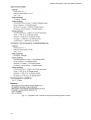
1
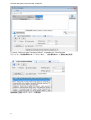
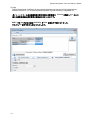
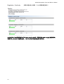
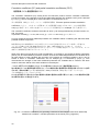
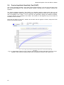
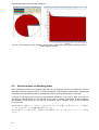
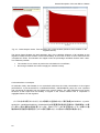
SML 5 - Software
General Description
SML5 和文取扱説明書
CONTACT
Swiss
Federal Office of Public Health
Food Safety Division
Schwarzenburgstrasse 165
3003 Bern
Switzerland
Tel.: +41 (0) 31 322 9568
Fax: +41 (0) 31 322 9574
http://www.bag.admin.ch
MDCTec Systems GmbH
Gutenbergstrasse 5
D-82205 Gilching
Germany
Tel.: +49 (0) 173 6662097
Fax: +49 (0) 3212 1029321
http://www.mdctec.com
email: [email protected]
AKTS AG
TECHNOArk 1
3960 Siders
Switzerland
Tel.: +41 (0) 848 800 221
Fax: +41 (0) 848 800 222
http://www.akts.com
[email protected]
General description of the new SML 5 software
Tableofcontents
この和文取扱説明書は ソフトウエアの操作説明を目的として作成されています。
原文の段落ごとに和文を挿入しています。和訳で分かりにくい場合は英文を参照してください。
英文マニュアルの
Introduction は別途
資料にまとめました。
株式会社パルメトリクス
2012-5-16
2
General description of the new SML software 5
1. SML5 ソフトウエアの操作の流れ
(別途詳細な説明が後半にあります。)
以下の 3~13 ページの解析例から解析フローを理解します。
1) Step 包装材の形状・寸法の決定
Software starts with definition of the packaging geometry - in this example the EU-cube:
包装材の形状・寸法を設定します。 この例はEU-cube
包装材のsurface(表面積):この例では600平方cmを入力します。
2) Step レイヤー数の定義
Define the number of layers - minimum two(2) for a monolayer plastic and the food/simulant
Add・Layerコマンドをクリックしてレイヤーの数を定義します。
レイヤー数の最小値は2となります。1個が単層プラスチックと1個が食品/擬似食品です。
もし包装材が4レイヤーならレイヤーの設定値は4+1=5とします。(重要1)
①
3
General description of the new SML 5 software
a) Layer 1 will be of type"Polymer" - POLYETHYLENE, LOW DENSITY from Database
a)レイヤー1のtypeとしてPolymerを選択します。
例ではDatabaseからPOLYETHYLENE, LOW DENSITYを選択しています。
データベースのpolymer選択画面
(b) Layer 1 / LDPE thickness e.g. 100 µm
(b)レイヤー1はLDPE厚みを100μmとします。厚みはカラムに数値を入力します。
4
General description of the new SML software 5
(c) Layer 2 will be of type "Contact medium" - vegetable oil - food simulant
(c) レイヤー2は接触媒体のタイプとなります。 食品擬似物として植物性油を選択
接触媒体を選択するデータベース画面例
5
General description of the new SML 5 software
(d) Layer 2 / Contact medium thickness calculated from volume over area of packaging
(d)レイヤー2/接触媒体の(平均)厚みは包装材面積を覆う体積から計算されます。
1000cm3 /600cm2 =1.6667cm
3) Step
Define the number of migrants - minimum one (1)
移行成分の数を定義します。最小値は1
この事例では移行成分の数を2としています。
6
General description of the new SML software 5
Substances are selected from the Database - e.g. Irganox 1076
データベースから物質を選択し、Assign to Layerをクリックします。例としてIrganox1076
(a) Substances 1 will be Irganox 1076
(a) 物質1はIrganox1076とします。
7
General description of the new SML 5 software
(b) Substances 2 will be Irgafos 168
(b) 物質2はIrgafos168とします。
4) Step
Define initial concentration of migrants in the polymer layer
- 100 ppm for Irganox 1076 - 500 ppm for Irgafos 168
ポリマーレイヤーの移行物質の初期濃度を定義します。
Irganox1076 100ppm
Irgafos168 500ppm
8
General description of the new SML software 5
4) Step
Define the estimation procedure for the diffusion coefficient of the migrants in the polymer layer
- e.g. selected Piringer approach
ポリマーレイヤーにおける移行物質の拡散係数を推定手順を選択定義します。
例えばPiringerアプローチを選択します。
9
General description of the new SML 5 software
5) Step
Define the partition coefficient of the migrants between polymer layer and food/simulant selected "known" K = 1 for both migrants because of good solubility in vegetable oil.
ポリマーレイヤーと食品疑似物間の移行物質の分配係数は
理由は植物性油脂は移行物質の溶解度が大きいためです。
Known を選択して 1 を入力
SML5 では Kp が未知の場合 Solubility や Pow を選択が可能になりました。
それでも Kp 値が不明ならば1を入力します。
10
General description of the new SML software 5
6) Step
Run prediction - e.g. at 40°C for 10 days
予測を実行します。 例40℃で10日間
Results
結果
グラフ縦軸の単位は mg/kg
11
General description of the new SML 5 software
Regislation Confirmity
法規の適合性の判断 (3つの規制値を表示)
EU およびスイスの規制値がいずれも SML:6mg/kg であり、予測結果の 0.5517mg/kg は規制値に
準拠する。Compliant は緑色表示、 non-Compliant は赤色表示となります。
12
General description of the new SML software 5
コンプライアンス証明書の生成 以下は証明書1ページ目の例
13
General description of the new SML 5 software
2. AKTS-SML5
SML5 の詳細な操作手順
以下の内容は SML5 ソフトウエアの Help コマンドに記載される内容とほぼ同じです。
2.1.
Basics
The use of AKTS-SML software can be described in four steps:
AKTS/SML ソフトウエアは以下の 4 つのステップで記述することができます。
1:パッケージの定義
2:温度条件の設定
3:計算結果の出力
4:予測結果の異なる規制に対する適合性
Fig. 0.1 - Applications of SML-Software from packaging definition to legislation conformity
1.
2.
3.
4.
Define the package by creating the different articles of the package and filling their properties.
Predict the migration using different temperature profiles (iso, non-iso, worldwide climate, etc.).
Analyze the calculated outputs.
Check the conformity of the results with different legislations.
1.
パッケージの異なる包装材を定義し、それらの各性質を入力してパッケージを定義します。
パッケージの定義とは
①食品包装材の形状を決定し、
②ソフトウエアに含まれるポリマーや化学物質のデータベースから包装材に使用されるポリマーを選択
実験的に求められた拡散係数と妥当性が評価されている値などが自動的に定義されます。
経験則により決定されたパラメータおよび対象物質の Tg 点温度や分子量理論を使って拡散係数を
求めます。
2.
異なる温度プロファイル条件を使って移行の予測(等温、非等温、世界気候条件など)
食品パッケージの加速試験や実際に使用されるなどの実験環境温度を設定します。
3.
計算結果出力の分析
4.
予測結果について異なる法規での適合性の点検
14
General description of the new SML software 5
2.2.
Package Structure パッケージ構造
A package is a group of different articles, each article having different layers properties. For instance a
bottle can be divided into two articles: the bottle cap and the bottle itself.
1つのパッケージは異なる包装材のグループでそれぞれの包装材は異なる層の性質を持っています。
例えばボトルは2つの包装材;ボトル・キャップとボトルそれ自身に分けられます。
Fig. 0.2 - A package can be composed of multiple articles
An article is composed of one or more layers of different sizes and properties.
1つの包装材は1つあるいは異なるサイズと性質をもつ複数の層で構成されます。
Fig. 0.3 - An article is composed of multiple
layers
包装材はマルチレイヤーで構成されています。
Fig. 0.4 - Chemicals can be found in all layers
化学物質はすべてのレイヤーに見受けられます。
Chemicals can be found in one or more layers.
化学物質は 1 個もしくはさらに多くのレイヤーに見受けられます。
注:ariticles の訳として物品・品目ですが、ここでは包装材と和訳します。
15
General description of the new SML 5 software
2.3.
Creating packages and articles
Fig. 0.5 - The package panel for packaging and article creation
以下は Fig.4-5 の赤枠内文章の和訳。
1 Package パッケージ
パッケージの形状を選択し、すべての包装材の数を入力します。
2 Layers レイヤー
すべての包装材に対するすべてのレイヤーを定義します。
3 物質
すべての包装材についてすべての移行物質を定義します。
4 データ
マス目のセルの中にすべてのレイヤーのすべての物質濃度、拡散係数、分配係数を入力します。
16
General description of the new SML software 5
The package panel allows changing the geometry and
the size of the package. The surface of each article can
be defined in the grid.
パッケージ・パネルは対象とするパッケージの寸法と構造を
変更することができます。
それぞれの包装材表面はマス目の中で定義されます。
Fig. 0.6 - The package panel
17
General description of the new SML 5 software
2.4.
The Wizard
When creating an article, many information and properties have to be filled. The role of the Article
Creation Wizard is to help filling all this information step by step.
包装材を設定するには、多くの情報と性質を設定する必要があります。それらの包装材を設定する“Article
Creation Wizard”はすべての情報をステップバイステップで設定することができます。
また Wizard を Close して Wizard なして設定することも可能です。
Fig. 0.7 - The wizard interface
1. Surface:
The surface of the article has to be entered first.
包装材表面積は最初に入力されなければなりません。
2. Layers
Then enter the number of layers and fill the information for each of them.
それからレイヤーの数を入力して、レイヤーそれぞれの情報を設定します。
3. Chemicals
Enter the number of chemicals and fill the information for each of them.
化学物質の数を入力し、それらの各情報を満たします
4. Data
First fill the concentration of each substance in each layer, then the diffusion
coefficients and finally the partition coefficient.
最初に各レイヤーのそれぞれの化学物質濃度、次に拡散係数、最後に分配係数を入力しま
す。
The package being fully created, it is possible to start calculating predictions by clicking on the 'Run
Prediction' button.
パッケージがすべて設定されたら、“Run Prediction”ボタンをクリックして予測計算をスタートさせます。
Note: the Wizard is optional.
18
Wizard 機能は選択可能です。
General description of the new SML software 5
2.5.
Article Properties 包装材の性質
The article grid
包装材グリッド(表入力欄)
Fig. 0.8 - The article grid
The article grid displays the layers (which can include the contact medium) and the substances. In the
grid it is possible to customize the concentration, the diffusion coefficient and the partition coefficient for
all chemicals and layers.
包装材のマス目はレイヤー(レイヤーと接触する媒体を含み)とそれらに含まれる物質を表示しています。
マス目の入力欄ですべての化学物質とレイヤーに対して濃度、拡散係数、分配係数をカストマイズすること
ができます。
The button Add Layer adds a new layer represented as a column in the grid.
The button Add Chemical adds a new chemical represented as a row in the grid.
Add Layer ボタンにより新しいレイヤーの列(column)をマス目入力欄へ加えることができます。
Add Chemical ボタンで新しい化学物質を行(row)に加えることができます。
See more about:
•
•
•
The layer properties ;
The chemical properties ;
The data (concentration and coefficients).
•
•
•
レイヤーの性質
化学物質の性質
それらのデータ(濃度と拡散係数や分配係数)
When all the properties of the article are filled, click on Run Prediction... to start a calculation process.
See the Predictions chapter for more information.
各包装材のすべての性質が入力されたとき、“Run Prediction”ボタンをクリックして計算プロセスをスタート
させます。さらに詳細な情報は Prediction の章を参照してください。
19
General description of the new SML 5 software
Layers
Fig. 0.9 - Layer properties
The layer properties panel allows defining the properties of the current selected layer.
Type (of layer) defines if the layer is a contact medium (typically food) or a polymer.
レイヤーの性質入力パネルは、現在選択されたレイヤーの性質を定義します。
(レイヤーの)タイプは、レイヤーが媒体(典型として食品など)に接触するのか、またはレイヤーがポリマー
に接触するのかを定義します。
Fig. 0.10 - Additional properties for polymer type layer
20
General description of the new SML software 5
Database allows browsing for a known polymer.
データベースは知られたポリマーをブラウジングして選択することができます。
約 240 種類
Fig. 0.11 - Polymer database
Contact medium
接触(食品)媒体
Fig. 0.12 - Contact medium database
Fig. 0.13 - Additional properties for contact medium type layer
21
General description of the new SML 5 software
Set to user defined allows customizing the properties of the polymer.
When the polymer is set to user defined, it is possible to enter the properties of the polymer. Otherwise
if the polymer is loaded from the database, its properties are filled automatically.
“ユーザ定義”をセットしてポリマーの性状をカストマイズすることができます。
ポリマーがユーザ定義にセットされるとそのポリマーの性質を入力することができます。
そうではなく、もしポリマーがデータベースからロードされると自動的にポリマーの性質が入力されます。
Reset layer allows setting the default values.
Reset layer をクリックするとデフォルト値にセットされます。
2.6.
Substances properties
Fig. 0.14 - Substance properties
The substance properties panel allows defining the properties of the current selected substance. When
the substance is set to user defined, it is possible to enter the properties of the substance. Otherwise if
the substance is loaded from the database, its properties are filled automatically.
物質性質パネル(画面)では現在、選択している物質の性質を定義することができます。
この Subustance を”set to user defined”をクリックすれば、その物質の性質を手動入力することができます。
そうではなく、もし Substance がデータベースからロードされると自動的にその物質の性質が入力されます。
22
General description of the new SML software 5
Database allows browsing for known substances (13'000 chemicals: additive, monomer, photoinitiator,
pigment, solvent, etc.).
データベースは既知の物質(13,000 の化学物質、光開始剤、顔料、溶媒、その他)をブラウジングすること
ができます。
Fig. 0.15 - Substance database
23
General description of the new SML 5 software
2.7.
Data – concentration, diffusion and partition coefficients
データ:濃度、拡散係数、および分配係数
The tab Data allows defining: データを選定することにより定義します
• the concentration ; 濃度
• the diffusion coefficient ; 拡散係数
• the partition coefficient. 分配係数
Diffusion coefficient
拡散係数
Fig. 0.16 - Determination of the diffusion coefficients. The data properties shown are based on the current
selected tab of the article grid.
The diffusion coefficient values can be entered manually when known, or it is possible to load a value
from the database, to use an Arrhenius, Piringer or Brandsch calculation and even to enter a customized
equation.
拡散係数値はもし値が既知であれば手動入力が可能です。
もしくはデータベースからアレニウス式、Piringer あるいは Brandsh による計算値を使うか、あるいはカ
ストマイズした式で入力することができます。
例ではプライマー層に含まれるメラニンに対して Brandsh を選択しています。
① Piringer と Brandsch 以外の手動入力はユーザがこれらの値を定義できる場合に使用します。
② ポリマーのデータベースは約 240 種類
(Version5.00 は解析機能が拡張され Brandsch 法による値を選択することが可能になりました。)
24
General description of the new SML software 5
補足説明
25
General description of the new SML 5 software
Partition coefficient 分配係数
Fig. 0.17 - Determination of the partition coefficients. The data properties shown are based on the current
selected tab of the article grid.
The partition coefficient value can be entered manually when known. In case of liquid contact media the
solubility can be entered, or the Pow.
分配係数値は値が既知であれば手動入力することができます。
接触媒体が液体である場合、溶解度を入力するか、あるいはその Pow を入力します。
Note
最も広く使用されている分配係数は、溶媒として n-オクタノールと 水を用いたオクタノール/水分配係数 で
あり、特に強調したい場合は Octanol / Water を意味する添字をつけ LogPow と略記される。LogPow
は物質の親水性・疎水性を判断する基礎的な数値として用いられ、医薬品の吸収率や生物学的利用能、
薬物受容体との疎水的相互作用のモデル化、土壌や地下水中での移動予測などに利用されている。
26
General description of the new SML software 5
3. Predictions and temperature profiles
予測と温度プロファイル
When all properties of an article are filled, it is possible to proceed with prediction calculations by clicking
on the prediction button.
すべて包装材の性質が入力されたとき、”Run prediction”ボタンをクリックすると予測計算を進行します
Fig. 0.1 - The prediction button
Different types of predictions are available:
以下に示すさまざまなタイプの予測が可能です。
•
•
•
•
•
•
•
•
3.1.
Isothermal
Non-Isothermal
Stepwise
Modulated
Shock
Worldwide
STANAG
Customized
Isothermal
等温条件
非等温条件
多段ステップ温度条件
周期的温度条件
熱衝撃的条件
世界気象温度条件
NATO の軍事的目的試験法の温度条件(SML では使わない)
ユーザ定義によるカストマイズ
等温条件
In the isothermal conditions mode, it is possible to set a number of isotherms and the temperature
difference (∆T) between each isotherm.
等温条件モードでは等温条件の設定数とそれぞれの等温条件の温度差を入力します。
Fig. 0.2 - Isothermal conditions
27
General description of the new SML 5 software
3.2.
Non-Isothermal 非等温条件
In the non-isothermal conditions, the starting temperature and different heating rates can be defined.
非等温条件においてはスタート温度と昇温速度を定義することができます。
Fig. 0.3 - Non-Isothermal conditions
3.3.
Stepwise
ステップワイズ
The stepwise conditions are a combination between isothermal and non-isothermal temperature modes.
A number of cycles can be also fixed.
ステップワイズとは等温条件と非等温条件の組合せモードです。
繰り返しサイクルの数も定義することができます。
Fig. 0.4 - Stepwise conditions
28
General description of the new SML software 5
3.4.
Modulated
モジュレート
In the modulated conditions, it is possible to set an oscillatory temperature mode, i.e. a day/night cycle.
モジュレートとはたとえば昼/夜サイクルの周期的な温度変動を設定することが可能です。
Fig. 0.5 - Modulated conditions
3.5.
Shock
The shock temperature conditions simulate a rapid temperature raise. The frequence of the temperature
shocks can be also defined.
温度ショック条件は高速な温度上昇をシミュレーションします。
温度ショックの周波数も定義することが可能です。
Fig. 0.6 - Shock conditions
29
General description of the new SML 5 software
3.6.
Worldwide
The worldwide temperature mode allows calculating predictions with real atmospheric temperatures. The
temperatures can be chosen for different climates (yearly temperature profiles with daily minimal and
maximal fluctuations).
Fig. 0.7 - Worldwide conditions
3.7.
STANAG
STANAG 2895 is a NATO Standardisation Agreement describing the principal climatic factors which
constitute the distinctive climatic environements found throughout the world.
Fig. 0.8 - STANAG conditions
30
General description of the new SML software 5
3.8.
Customized
The customized prediction mode allows loading a file with a custom temperature profile, i.e. when using a
datalogger.
Fig. 0.9 - Customized conditions
Prediction と温度プロファイルの機能は AKTS ソフトウエアに共通機能です。
とくに 3.1,
31
3.3,
3.4,
3.6,
3.8 の温度プロファイルの設定方法を理解する。
General description of the new SML 5 software
Outputs
出力
The output window shows the results of the prediction calculations. The window is divided in three parts:
“Output window”は予測計算の結果を表示します。
この window は3つの部分に分けられます。
•
•
•
The results grid;
The c(t) chart;
The c(x, t) chart.
結果
濃度(t)チャート
濃度(x,t)チャート
Moving the mouse pointer over the c(t) chart will update the results grid and the c(x, t) chart based on the
time pointed on the c(t) chart.
C(t)チャート上のマウス・ポインターを動かすことにより、c(t)チャートで設定された時間に基づいて結
果グリッド(マス目)、c(x,t)チャートが変更されます。
Fig. 0.1 - The result grid c(t)
The grid shows the values of the concentration, the diffusion coefficients and the partition coefficients for
all substances in all layers.
マス目はすべてのレイヤーの物質に対する濃度、拡散係数と分配係数を示します。
32
General description of the new SML software 5
3.9.
The c(t) chart
Fig. 0.2 - The c(t) chart
The c(t) chart shows the migration of the chemicals over time. The chemicals and layers to be displayed
can be selected by using the checkboxes in the results grid.
C(t)は時間に対応する化学物質の移行を示します。
表示される化学物質と層は result grid(結果マス目表示の上部)にある check box を使って選択するこ
とができます。
33
General description of the new SML 5 software
3.10. The c(x,t) chart
上の表示の濃度軸を拡大表示すると下段の表示になります。
(Zoomed)
Fig. 0.3 - The c(x, t) chart
The c(x, t) chart shows the migration of the chemicals into the different layers, the dotted line being the
average concentration of a chemical inside a layer.
c(x,t)チャートは異なる層へ化学物質が移行することを示し、破線ラインは層内の化学物質の平均濃度を
示します。
34
General description of the new SML software 5
3.11. Comparison Output
比較表示出力
The comparison output window allows comparing the calculation results of different outputs. To add an
output to the comparison, drag and drop the output from the list on the left to the dedicated zone in the
comparison output window.
比較表示出力は異なる出力の計算結果を比較することが可能になります
Fig. 0.4 - The comparison output window
35
General description of the new SML 5 software
3.12. Sum Output 合計出力
The sum output window allows adding the calculation results of outputs of same substances. To add an
output to the comparison, drag and drop the output from the list on the left to the dedicated zone in the
comparison output window.
sum output(合計出力)は同じ物質の出力の計算結果を加えることが可能になります。
1つの結果を比較に加えて、左のリストから出力を比較出力(comparison output)の中にある関係す
るゾーンをドラック&ドロップします。
Fig. 0.5 - The sum output window
36
General description of the new SML software 5
4. Legislation
and compliance
法規と整合性
In the last years migration modelling got more and more accepted and was introduced in legislation for
plastic food contact materials and articles allowing for compliance assessment with applicable specific
migration limits stipulated by legislation.
昨年 2011 年において移行モデルがさらに受け入れられるようになり、プラスチック食品接触物質と
それらの事項に対して法規に持ち込まれ、法規により適用される特定移行限界(SML)が明記されるよ
うになりました
Legislation conformity check: Compliance evaluation for substances with specific migration limit (SML)
listed in the Plastics Regulation (EU) No 10/2011 and generation of compliance certificates.
法規適合性の点検
プラスチック規制(EU NO.10/2011)にリストされた SML の物質に対するコンプライアンス評価
およびコンプライアンス証明書の生成
37
General description of the new SML 5 software
38
General description of the new SML software 5
39
General description of the new SML 5 software
Fig. 4.1 - Legislation and compliance report (calculated migration values)
40
General description of the new SML software 5
Fig. 4.2 - Legislation and compliance report (migration limits)
41
General description of the new SML 5 software
5.
Sensitivity Analysis Methods
5.1.
感度分析の手法
Introduction
Sensitivity analysis studies how the uncertainties in the model inputs (X1;X2;…;Xk) affect the model's
response Y, which (for simplicity) we assume to be a scalar:
Y = f(X1;X2; … ;Xk);
where f describes the implemented model.
A sensitivity analysis attempts to provide a ranking of the model's input assumptions with respect to their
contribution to model output variability or uncertainty. The difficulty of a sensitivity analysis increases
when the underlying model is nonlinear, nonmonotonic or when the input parameters range over several
orders of magnitude. Many measures of sensitivity have been proposed. For example, the partial rank
correlation coefficient and standardized rank regression coefficient have been found to be useful. Scatter
plots of the output against each of the model inputs can be a very effective tool for identifying sensitivities,
especially when the relationships are nonlinear. In a broader sense, sensitivity can refer to how
conclusions may change if models, data, or assessment assumptions are changed, see [1] for more
details on the subject.
感度分析はモデルの出力変動あるいは不確実性に関してそのモデルの入力した仮定についてランクをつ
けすることを試みます。
感度分析の困難さは非直線性や非単調性あるいは入力パラメータが数桁を越えるような場合です。
感度の多くの測定することが提案されてきました。
例えば部分的なランク補正係数と標準化ランク回帰係数が有望であることが分かってきました。
それぞれのモデル入力に対する分散プロットは感度を同定するには非常に効果的なツールであり、
とくにそれらの関係が非直線性であるとき有効です。
広義的には“感度分析”は、もしモデル、データあるいはアセスメントの仮定が変化すると、どのようにその
結論が変化するか?を参照することができます。
The analysis methods available in SML software are:
SML5 ソフトウエアにおいては感度分析手法が可能であり
•
•
•
42
Monte Carlo
モン手・カルロ法
Fourier Amplitude Sensitivity Test (FAST) 高速フーリエ増幅感度テスト(FAST)
Sobol
ソボル
General description of the new SML software 5
5.2.
Monte Carlo Simulation (MCS) モンテ・カルロ・シミュレーション
Monte Carlo Simulation (MCS) is a widely used method for uncertainty or sensitivity analysis.
It involves random sampling from the distribution of inputs and successive model runs until the desired
accuracy of the outputs is reached. Not only the means and variances but also the distributions of input
parameters are required to run the MCS. In the present version of SML only Gaussian (normal)
distribution have been implemented for the different input parameters.
モンテカルロ・シュミレーション(MCS)は不確実性あるいは感度分析に対して広く使用されている手法です。そ
れは入力の分布からランダム・サンプリングを必要とし、出力の精度が希望するところまで逐次モデルを実行しま
す。変動と平均のみならず、入力パラメータの分布がMCSを計算するために要求されます。
SML5現在バージョンは、異なる入力パラメータに対してガウス関数(ノーマル)分布法のみが導入されています。
Fig. 5.1 - Random sampling from the distribution of inputs (Gaussian (normal) distribution).
訳注:誤差分析をするには入力パラメータにGaussianを選択して誤差範囲を入力します。
mはmean値、sはstandard deviation値
レイヤーの厚みや移行物質の含有量mg/kg値、溶解度のばらつきに対してどの項目が最も結果に影響を及
ぼしているかを調べることができます。
The main advantage of the MCS is its general applicability. MCS suffers for its computational
requirements since thousands of repetitive runs of a model are required to reach convergence. Highspeed personal computers have minimized the computational challenges. Another limitation of MCS is
the need for user-specified rules for determining the number of simulations required, see [2-4] for more
information and recommendation on the subject.
MCSのおもな優位点はその一般的な適用性にあります。MCSは1つのモデルに対して結果が収束に達す
るには数1000回の繰り返し計算が要求されるためコンピュータ計算能力が要求されます。
MCSの別の制限はuser-specified(ユーザが定義しなければならない点)です。
この課題についてのさらなる情報と推奨は最終頁にある文献(2-4)をご覧ください。
e-words.jp より
MCS モンテカルロ法:
乱数を用いたシミュレーションを何度も行うことにより近似解を求める計算手法。
解析的に解くことができない問題でも、十分多くの回数シミュレーションを繰り返すことにより、近似的に解を求め
ることができる。適用範囲が広く、問題によっては他の数値計算手法より簡単に適用できるが、高い精度を得よう
とすれば計算回数が膨大になってしまうという弱点もある。
43
General description of the new SML 5 software
Fig. 5.2 - Quantification of the amount of variance that each input factor Xi (all variables of the articles)
contributes with on the unconditional variance of the output V (Y).
Sensitivity measures based on the MCS approach include regression-based measures (Standardized
Regression Coefficients (SRC), Partial Correlation Coefficients (PCC), Standardized Rank Regression
Coefficients (SRRC), Partial Rank Correlation Coefficients (PRCC)). Some of them have been
implemented in the present version of SML and are described below.
MCSアプローチに基づく感度分析手段は回帰に基づく手段;標準回帰係数、偏相関係数、標準順位相関係数、
偏順位相関係数を含みます。
これらのいくつかは現バージョンのSML5ソフトウエアに導入されています。
SRC
PCC
SRCC
PRCC
44
標準回帰係数
偏相関係数
標準順位相関係数
偏順位相関係数
General description of the new SML software 5
Correlation coefficient (CC) and partial correlation coefficients (PCC)
相関係数(CC)と偏相関係数(PCC)
The correlation coefficients (CC) usually known as Pearson's product moment correlation coefficients,
provide a measure of the strength of the linear relationship between two variables x and y and is denoted
by corr(x; y), see for example [5] for more information on the definition of CC.
単に相関係数(CC)といえば、ピアソンの積率相関係数(Pearson product-moment correlation
coefficient)をさし、これは2つの変数 X と Y の直線関係の強さの目安であり、x.y の相関係数
corr(x,y)に依存します。CC の定義についてのさらなる情報は巻末の example(5)を参照のこと
The correlation coefficient measures the extent to which y can be approximated by a linear function of x,
and vice versa.
In particular if exactly y = a + bx, then corr(x; y) = 1, if b = 1 and corr(x; y) = -1, if b = -1.
CC only measures the linear relationship between two variables without considering the effect that other
possible variables might have.
相関係数はyがxの直線関数および逆の場合も同じでほぼ近似値が得られるように拡張して評価する。
とくにもし正確にy = a + bx, then corr(x; y) = 1, if b = 1 and corr(x; y) = -1, if b = -1. であれば
CC(相関係数)は他の可能な変数があるかもしれないことの効果を考慮することをしなければ、2つの
変数から直線関係を評価するだけになってしまう。
When more than one input factor is under consideration, as it usually is, the partial correlation coefficients
(PCCs) can be used instead to provide a measure of the linear relationships between two variables when
all linear effects of other variables are removed. PCC between an individual variable xi and y can be
written in terms of correlation coefficients, see for example [5]. It is denoted by pcc(xi; y). PCC
characterizes the strength of the linear relationship between two variables after a correction has been
made for the linear effects of the other variables in the analyses.
1つの入力因子以上が考慮されたとき、それは通常のことなのですが、偏相関係数(PCCs)は
他の変数のすべての直線的効果が除かれて、2つの変数の間の直線関係の評価を提供する代わりに使用
されます。固有の変数xとyの間の偏相関係数(PCC)は相関係数(CC)に関して書くことができる。
それはPCC(x,y)によって表示されます。
PCCはある補正が分析のなかで他の直線的な変数の直線的な効果が寄与したあと、2つの変数間の直線
的な関係の度合いの特性を示します。
Fig. 5.3 – Correlation coefficients (CC) providing a measure of the strength of the linear relationship
between two variables x (variable parameters in the article) and y (migration).
45
General description of the new SML 5 software
Fig. 5.4 - Scatter plots illustrating relationships between the input factor Xi (variable parameters in the
article) and the output Y (migration).
入力因子 Xi(包装材条件における変数パラメータ)と出力 Y(移行)の分散プロット
訳注:右下の表示グラフは相関があることを意味する。他のグラフには相関は認められない。
A plot of the points [Xij ; Yj ] for j = 1; 2;…;N usually called a scatter plot can reveal nonlinear or other
unexpected relationships between the input factor Xi and the output Y. Scatter plots are undoubtedly the
simplest sensitivity analysis technique and is a natural starting point in the analysis of a complex model. It
facilitates the understanding of model behavior and the planning of more sophisticated sensitivity analysis.
ポイント [Xij ; Yj ] for j = 1; 2;…;N は通常分散プロットと呼ばれ、入力因子Xi と出力 Y.の間の非直線または
他の予期しない関係を浮き彫りにします。分散プロットは疑いもなく、最もシンプルな感度分析技術であり、
複雑なモデル分析で自然な出発点となります。モデルの振る舞いの理解を容易にし、さらに洗練された感
度分析の設計立案が可能になります。
46
General description of the new SML software 5
Rank correlation coefficient (RCC) and partial rank correlation coefficients (PRCC)
順位補正係数(RCC)と分配順位補正係数(PRCC)
Since the correlation coefficient and partial rank correlation coefficient methods are based on the
assumption of linear relationships between the input-output factors, they will perform poorly if the
relationships are nonlinear. With SML-Software, rank transformation of the data is possible too. This
concept can be used to transform a nonlinear but monotonic relationship to a linear relationship. When
using rank transformation the data is replaced with their corresponding ranks. The usual correlation
procedures are then performed on the ranks instead of the original data values. Spearman rank
correlation coefficient (RCC) are corresponding CC calculated on ranks and partial rank correlation
coefficients (PRCC) are PCC calculated on ranks.
相関係数と偏相関係数法は入力・出力因子間の直線関係を仮定することが基礎となっており、もしその関
係が非直線であるとすると、これらの手法からは貧しい結果しか得られません。
SML5ソフトウエアではデータ順位変化も可能となっています。この概念は単調でない非直線関係から直線
関係に変換するのに使用されます。
通常の補正手順はオリジナルデータの値の代わりにそのランク上で実行されます。
Spearman順位補正係数(RCC)は順位上で計算されたCCであり、分配順位補正係数(PRCC)は順位上で計
算されたPCCです。
Rank transformed statistics are more robust, and provide a useful solution in the presence of long tailed
input-output distributions. A rank transformed model is not only more linear, it is also more additive. Thus
the relative weight of the first-order terms is increased on the expense of higher-order terms and
interactions see for example [5].
順位変換統計はさらに粗野(あらっぼい)手法で、長い尾を有する入力・出力分布がある場合には有効な解
決法です。
1つの順位変換モデルはさらに直線的ではないばかりではなく、よりadditive(加法的)です。
このように1次項の相対的な重みは例(5)のように高次のexpense上で増加し、干渉します。
(この項は統計学の知識がないと理解不能?)
47
General description of the new SML 5 software
5.3.
Variance based methods for sensitivity analysis
感度分析に対する分散基礎方式
The main idea of the variance-based methods is to quantify the amount of variance that each input factor
Xi contributes with on the unconditional variance of the output V (Y).
分散基礎方式の主な考え方はそれぞれの入力因子;Xi は出力V(Y)の無条件的な分散に寄与しているとい
うことにあります。
We are considering the model function: Y = f(X), where Y is the output and X = (X1;X2;… ;Xk) are k
independent input factors, each one varying over its own probability density function. The values of the
input parameters are not exactly known. We assume that this uncertainty can be handled by using
random variables Xj , j = 1;…; k of known distributions. Then the model output is also a random variable Y
= f(X1; : : : ;Xk).
われわれはモデル関数Y = f(X),Y はその出力、そしてX = (X1;X2;… ;Xk)はkに独立した入力因子であり、そ
れぞれの変動を越えるのはそれ自身の確率密度関数であると考えます。
入力パラメータの値は不明です。この不確定さはランダム変数Xj , j = 1;…;(k既知の分配)を使うことにより
取り扱うことができると仮定します。またこのモデル出力はランダム変数Y = f(X1; : : : ;Xk).です。
The first order effect for the input factor j is the fraction of the variance of the output Y which can be
attributed to the input Xj and is denoted by Sj , see for example [5].
入力因子j に対する1次の影響は出力Yの変数のゆらぎであり、Yは入力Xj に起因し、Sj によって表示されま
す。例 [5] を参照
To estimate the value of Sj we require realizations of the input distributions and the associated model
evaluations. The ratio Si was named first order sensitivity index by Sobol [6]. The first order sensitivity
index measures only the main effect contribution of each input parameter on the output variance. It
doesn't take into account the interactions between input factors. Two factors are said to interact if their
total effect on the output isn't the sum of their first order effects. The effect of the interaction between two
orthogonal factors Xi and Xj on the output Y can be computed (see for more details [5]) and is known as
the second order effect. Higher-order effects can as well be computed, see for example [5].
Sj の値を推定するためには、われわれは入力値が分散するという認識とそれに対応するモデルを評価する
ことが要求されます。そのSi レシオはSobol [6].によって一次感度指標と呼称されています。
1次感度指標とは出力変動に基づいてそれぞれの入力パラメータの主となる影響の寄与だけを評価するも
のです。入力因子間の干渉を計算することはしません。もし出力に対する全体の影響が1次的影響の合計
でないとすれば、2つの因子は相互に作用していることになります。
2つの直交する因子Xi と出力Xj が計算され、2次オーダの影響として判明されます。同様に高次の影響も
計算されることが可能です。
A model without interactions is said to be additive, for example a linear one. The first order indices sums
up to one in an additive model with orthogonal inputs. For additive models, the first order indices coincide
with what can be obtained with regression methods. For non-additive models we would like to know
information from all interactions as well as the first order effect. For non-linear models the sum of all first
order indices can be very low.
相互作用なしのモデルというのは加法、例えば直線的であると言えます。
1次オーダ指標は1つの直交的な入力を伴う1つの加法モデルの中に1つとして合計するものです。
加法モデルに対して。1次オーダ指標は回帰法で得られるものと一致します。
非加法モデルに対してすべての1次オーダ指標の合計は非常に遅いものであると言えます。
The sum of all the order effects that a factor accounts for is called the 'total' effect [7]. So for an input Xi,
the total sensitivity index STi is defined as the sum of all indices relating to Xi (first and higher order).
すべてのオーダ次数の影響合計は合計影響と呼ばれる因子とみなされます。
1つの因子Xi は合計感度指標 STi は Xi(1次および高次)に関係するすべての指標の合計として定義されます.
48
General description of the new SML software 5
There are different techniques to obtain these sensitivity indices, such as Sobol's indices, Jansen's
Winding Stairs technique, (Extended) Fourier Amplitude Sensitivity Test ((E)FAST).
Sobolの指標、Jansen Winding Stairs あるいは拡張Fourier Amplitude Sensitivity Testのようにこれらの感
度指標を得るためには異なったテクニックがあります。
訳注:
計算モデルの入力変数に不確実さが存在する場合に,入力変数の不確実さがモデル中で伝播し,モデルの出力変数の
不確実さを引き起こす.FAST(Fourier Amplitude Sensitivity Test)手法は,モデルの入力変数の不確実さによる出力変
数の不確実さへの影響を評価する手法であり,グローバル感度解析としては最初に提案されたものです。
In the present software, two methods are implemented, the FAST method and the Sobol's indices based
on Jansen's Winding Stairs technique.
SML5現ソフトウエアは2つの手法、FAST(Fourier Amplitude Sensitivity Test)と Jansen's Winding Stairs
技法を基礎とするSobol指標を採用しています。
49
General description of the new SML 5 software
5.4.
Fourier Amplitude Sensitivity Test (FAST)
The Fourier Amplitude Sensitivity Test (FAST) was proposed already in the 70's [8-10] and was at the
time successfully applied to two chemical reaction systems involving sets of coupled, nonlinear rate
equations.
The Fourier Amplitude Sensitivity Test (FAST) is a sensitivity analysis method which does not use
a Gaussian distribution. Rotating vectors are assigned to each variable, and each has a unique frequency
and an amplitude of the "mean". A lot of input sets are generated, making the variables oscillating.
A Fourier analysis is then applied on the results. The number of runs depends only on the number of
variables, but it is not linear.
Note that the graphs of the FAST method are the same than the graphs of Sobol, except that FAST
shows only the local sensitivity.
Fig. 5.5 - Quantification based on FAST analysis of the amount of variance that each input factor Xi (all
variables of the articles) contributes with on the unconditional variance of the output V (Y).
50
General description of the new SML software 5
Fig. 5.6 - FAST analysis results. Sensitivity S(v) of each variable (influence of each examined variable
on the migration results)
5.5.
Sobol's indices via Winding Stairs
Chan, Saltelli and Tarantola [11] proposed the use of a new sampling scheme to compute both first and
total order sensitivity indices in only N x k model evaluations. The sampling method used to measure the
main effect was called Winding Stairs, developed by Jansen, Rossing and Deemen in 1994 [12].
A first set of variables simply comes from the Gaussian distribution. Then a lot of other set of input of
variables are generated from the first set and will be used in complex mathematics analysis afterward
(For example: if one enters 10 runs and has 1 substance with 4 variables, it will run the simulations
(4+1)*10 times).
変数を単純化する最初のセットはガウス分布に由来します。他の変数入力の他の多くのセットは最初の
セットから生成され、その後複雑な数値分析を行います。
例えば 1 個の入力で 10 回計算し、4 変数で 1 個の物質なら(4+1)×10 回のシミュレーション計算を
します。
51
General description of the new SML 5 software
Fig. 5.7 - Sobol analysis results. Total sensitivity St(v) of the variables (influence of all variables on the
migration results)
The above figures illustrate the total sensitivity St(v) of the variables (influence of all variables on the
migration results) and the evolution of the total sensitivity as a function of time. In some cases there are
"unexplained" values. This situation can happen when the percentage calculation doesn't reach 100%.
Two cases are possible:
•
•
The number of runs chosen to perform the calculations is not sufficient;
Not enough variables are chosen to apply the method correctly.
Comments about our example:
All methods clearly demonstrate for our examined article that the initial concentration of the migrant
(OCTADECYL 3-(3,5-DI-tert-BUTYL-4-HYDROXYPHENYL) PROPIONATE) plays the most important
role concerning its migration from the article to the contact medium. The other parameters such as the
thickness of both layers and the solubility of migrant in the contact medium have in comparison a
negligible influence on the migration.
すべての方式は明らかにわたくしたちが試験した包装材に対して移行物質(OCTADECYL 3-(3,5-DItert-BUTYL-4-HYDROXYPHENYL) PROPIONATE)の初期濃度は接食品包装材から触媒媒体への移
行に関して最も重要な役割を演じています。他のパラメータである両方のレイヤーの厚みや接
触媒体の移行物質の溶解度などはこの移行現象に対して比較すれば影響が無視できる。
52
General description of the new SML software 5
[1] A. Saltelli, K. Chan, M. Scott (Eds.). Sensitivity Analysis Probability and Statistics Series, John Wiley
and Sons, 2000.
[2] J. C. Helton, F. J. Davis. Sampling Based Methods. Chapter 6 in Mathematical and Statistical Methods
for Sensitivity Analysis of Model Output. Edited by A. Saltelli, K. Chan, and M. Scott, John Wiley and
Sons, 2000.
[3] Helton J. C. Uncertainty and sensitivity analysis techniques for use in performance assessment for
radioactive waste disposal. Reliability Engineering and System Safety, 42, 327 - 367, 1993.
[4] http://www.epa.gov/reg3hwmd/risk/human/info/guide1.htm
[5] P.-A. Ektr. om. Eikos, A simulation toolbox for sensitivity analysis, degree project, 2005.
[6] I. M. Sobol'. Sensitivity analysis for nonlinear mathematical models. Mathematical Modeling and
Computational Experiment, 1, 407 - 414, 1993.
[7] T. Homma and A. Saltelli. Importance measure in global sensitivity analysis of nonlinear models.
Reliability Engineering and System Safety, 52, 1 - 7, 1996.
[8] R. I. Cukier, C. M. Fortuin, Kurt E. Shuler, A. G. Petschek, and J. H. Schaibly. Study of the sensitivity
of coupled reaction systems to uncertainties in rate coefficients. I theory. The Journal of Chemical
Physics, 59, 3873 - 3878, 1973.
[9] J. H. Schaibly and Kurt E. Shuler. Study of the sensitivity of coupled reaction systems to uncertainties
in rate coefficients. II applications. The Journal of Chemical Physics, 59, 3879 - 3888, 1973.
[10] R. I. Cukier, J. H. Schaibly, and Kurt E. Shuler. Study of the sensitivity of coupled reaction systems to
uncertainties in rate coefficients. III analysis of the approximations. The Journal of Chemical Physics,
63, 1140 - 1149, 1975.
[11] Karen Chan, Andrea Saltelli, and Stefano Tarantola. Winding stairs: A sampling tool to compute
sensitivity indices. Statistics and Computing, 10, 187 - 196, 2000.
[12] M.J.W. Jansen, W.A.H. Rossing, and R.A. Daamen. Monte Carlo estimation of uncertainty
contributions from several independent multivariate sources. Predictability and Nonlinear Modelling in
Natural Sciences and Economics, 334 - 343, 1994.
53