Download MetCor User Guide - Department of Chemistry

MetCor User Guide
Developer: Ankit Rastogi
McMaster University, Department of Chemistry
1280 Main St. W, Hamilton, Ontario, Canada L8S 4M1
Table of Contents:
1.0
Copyright Notice and Disclaimer………………………………………………….
1
2.0
Overview
2.1
Models and Visualization……………………………………………………..
2
3.0
Installation
3.1
Minimum Hardware Requirements………………………………………..... 4
3.2
Supported Operating Systems and Required Libraries…………………… 4
4.0
Basic Operation
4.1
Overview and Flowchart………………………………………………………
4.2
Endpoint Files and Directories……………………………………………….
4.3
The Correlation Data File
4.3.1
Purpose and Overview……………………………………………...
4.3.2
Formatting Guidelines and Requirements………………………..
4.3.3
Time Zone Correction with Daylight Savings Offset…………….
4.4
Output Files and Directories Structure……………………………………...
4.5
Back Trajectory Time Intervals………………………………………………
4.6
Spatial Extent and Grid Resolution….………………………………………
4.6.1
Presets……………………………………………………………….
4.6.2
Customization……………………………………………………….
4.7
PSCF
4.7.1
Setting Threshold Values…………………………………………..
4.7.2
Weighting Table and Types of Weighting………………………..
4.7.3
PSCF Output Matrices……………………………………………...
4.8
Additional Tools
4.8.1
Elevation Plot Tool…………………………………………………..
4.8.2
Grid Population Histogram Data…………………………………...
4.8.3
PSCF Scatter Data…………………………………………...……..
4.8.4
GNUPlot Script for Visualization…………………………………...
4.9
Running and Stopping Jobs on MetCor…..………………………………...
5.0
6.0
7.0
8.0
Advanced Tools
5.1
Using Configuration (*.cfg) files
5.1.1
Syntax and Format……...…………………………………………..
5.1.2
Loading a *.cfg file on MetCor 1.0…………………………………
Quick GUI Reference………………………………………………………………...
Examples
7.1
Mapping Pollution Data……………………………………………………….
7.2
Plotting Multiple Trajectories…………………………………………………
Troubleshooting
8.1
Form Input Errors……………………………………………………………...
8.2
Errors During Calculations……………………………………………………
8.3
Premature Termination………………………………………………………..
5
6
7
7
8
9
9
9
10
10
11
11
12
12
13
13
14
14
16
17
18
21
22
23
24
24
Page 1
1.0 Copyright Notice and Disclaimer
COPYRIGHT NOTICE:
Copyright (c) 2010 Ankit Rastogi. All rights reserved.
McMaster University, Department of Chemistry
1280 Main St. W., Hamilton, Ontario, Canada L8S 4M1
DEFINITIONS
1. "Installation Package" shall mean all files contained in the "MetCor_setup.exe" file.
2.
"Package" shall mean all of the files contained in the Installation Package except those explicitly belonging to the Java Runtime
Environment and those under the folder entitled "lib".
3.
"Software" shall mean an installed copy of this Package.
4.
"Modification" shall mean any provisions made to the Software or this Package. Modifications include but are not limited to changes in
the Software's source code which change the output and behaviour of the Software.
5.
"Modified Package" shall mean a derivative of the Package created as a result of one or more Modification applied to the Software
and/or Package.
6.
“Distribution” shall mean allowing one or more other people to in any way download or receive a copy of this Package, Modified
Package or Installation Package.
7.
“Author” shall mean the copyright holder of the Software, Package and Installation Package.
8.
“You” shall mean an individual or Legal Entity exercising permissions granted by this Copyright Notice and Disclaimer.
AGREEMENT
1. Permission to use this Software and/or Package is hereby granted, provided that:
a) Copyright notices within source files and within this Package are retained and unchanged.
b) Use of this Software and/or Package for published work must contain at the very least the following citation:
MetCor downloaded at http://www.chemistry.mcmaster.ca/people/faculty/mccarry/MetCor.html and developed by Ankit Rastogi.
2. Permission to make Modifications to this Software or Package requires explicit permission from the Author.
3. Permission to Distribute this Software and/or Package is hereby granted, provided that:
a) Any Distribution of this Package includes this Copyright Notice and Disclaimer and is released under the terms of this Agreement.
b) This Package and Modified Packages may not be Distributed or Sold under a paid license.
DISCLAIMER
This software is provided "as is" without express or implied warranty to the extent permitted by applicable law. In no event shall the author be
liable to any party for any direct, indirect, incidental, special, exemplary, or consequential damages arising in any way out of the use or
misuse of this Package and/or Software.
1.0 – Copyright Notice and Disclaimer
Page 2
2.0 Overview
MetCor (Meteorological Correlation) contains a suite of tools used in the analysis of data
contained in geospatial coordinates. Geospatial coordinates can exist as endpoints in
meteorological backward or forward trajectories in the Canadian Meteorological Centre (CMC)
3-dimensional or Hybrid Single Particle Lagrangian Integrated Trajectory Model (HYSPLIT)
format. Data is added to these geospatial coordinates on the basis of a unique identifier given
to points belonging to the same back trajectory. The identifier in the CMC and the HYSPLIT
format is the back trajectory starting date.
In addition to histogram tools and elevations for endpoint analysis, MetCor is mainly used in
conjunction with correlated data for the calculation of Particle Source Contribution Function
(PSCF) value matrices. These matrices can be visualized by geographical information system
(GIS) software.
The following subsection describes how endpoints are organized and how PSCF values are
calculated in MetCor.
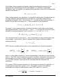
2.1 Models and Visualization
Upon extracting endpoints from trajectories, MetCor organizes these points into an array of
grids with finite area meant to represent all or part of the world. The area of the grid is
specified by a single grid’s length and width in latitude and longitude degrees, respectively.
dx
(0o, 0o)
(1o, 0o)
dy
(0o, 1o)
(1o, 1o)
Figure 1: A representation of a part of the world by an array of grids. Latitude and Longitude Degrees are used as units here.
A single grid’s geospatial coordinates are represented by the latitude and longitude of its topleft corner. Each grid in the array has a uniform size specified by dx and dy such that:
{dx ∈ R ^ dy ∈ R | dx > 0 ^ dy > 0}
2.0 – Overview
Page 3
On the basis of their geospatial coordinates, endpoints are abstractly arranged into the
appropriate grid representing the world. Each endpoint, P is defined by its geospatial
coordinates x and y, an identifier k, an optional starting elevation e and a set of correlated data
specific to the identifier, Ck:
Pk ,e = ( xk ,e , yk ,e , Ck )
When loading endpoints from trajectories, k is typically the starting date of the back trajectory
and data is added to appropriate points on the basis of k. A grid can be defined by the
geospatial coordinates xo and yo, a set of points {Pk,e}, the grid resolution and the number of
points in the grid with a non-empty set Ck, n (also known as the “grid population”).
G = ( xo , yo , dx, dy , {Pk ,e }, n). n ∈ I | n > 0
The world, W, can be represented by a 2-dimensional matrix of grids with a corner latitude
and longitude defined by i and j such that xo = i and yo = j. W can span all or part of the world,
defined by a maximum longitude X and Y such that 0 < X ≤ 360 and −90 < Y ≤ 90 .
W = [Gij ] = [ xoij , yoij , dx, dy, {Pk ,e }ij , nij ]
The concentration data for each point, Ck, can be represented as a pair containing the name
of the variable, s and its value v, where #b represents the number of different variables
existing in the set Ck.
C k = {s b , v bk }/ b#b=0
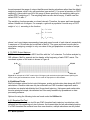
PSCF value for a variable with the name s can be calculated for W the by the expression:
 mij 
[ PSCFij ]sb = w(nij )  
 nij 
OR
 mij 
[ PSCFij ]sb = w(# k , e in G ij )  
 nij 
where mij is the number of points in Gij whose corresponding vbk falls above or at a threshold
value vbT. The PSCF value is weighted by a positive, real value w obtained as a function of the
grid population or the number of unique identifiers and starting elevations in a grid itself (#k,e
in Gij). In PSCF analyses, only the points with correlated data are considered in all
calculations.
The number of PSCF matrices is therefore #b. It is important to note that for a grid with nij = 0
a meaningless no-data value is given to PSCFij. The number of grids in the world and
consequently the number of data elements in each PSCF matrix is #G, given by:
 X  Y 
# G =    ∋ X mod dx = Y mod dy = 0
 dx  dy 
2.0 – Overview
Page 4
3.0 Installation Procedure
3.1 Minimum Hardware Requirements
According to the requirements of a calculation or “job” as outlined in section 2.0, MetCor
required different amounts of computational resources. The memory used depends most
significantly on grid resolution (section 4.6) and the number of variables in analysis (section
yet also on the number of trajectories being analyzed.
The chart below shows minimum and recommended hardware requirements for MetCor
calculations:
Minimum
Recommended
Processor
800 MHz (single core)
1.0 GHz (multi-core)
Physical Memory (RAM)
512 MB*
3.0 GB
Free Hard Drive Space
500 MB
4 GB
Monitor Resolution
1024 x 768 px.
1280 x 800 px.
*limits calculation jobs to lower grid resolutions and smaller spatial extent
3.2 Supported Operating Systems and Required Libraries
The following operating systems have been tested with MetCor:
Windows-based Operating Systems:
- Microsoft Windows (Windows 7, Windows Vista, Windows XP, Windows 2000)
Unix-based Operating Systems:
- Ubuntu Linux (versions 8.04, 8.10, 9.04, 9.10, 10.04)
- Mac OS X (versions 10.5, 10.6)
Provided that the minimum hardware requirements are met, any operating system which
supports the Java Runtime Environment (version 1.6.0) should be able to run MetCor without
issue.
Installation instructions for running MetCor each platform can be found in the README file
associated with the setup.exe file (for Windows based operating systems) or .tar.gz file (for
Unix based operating systems). The same README file is found in the installation directory.
It also contains information on setting up shortcuts and launchers for Unix-based operating
systems.
The amount of memory which MetCor uses depends on the operating system in use. In
Windows based operating systems, MetCor will use anywhere from 25% to 100% of free
available memory. The amount of memory installed for Unix-based operating systems is user
defined.
3.0 – Installation
Page 5
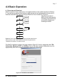
4.0 Basic Operation
4.1 Overview and Flowchart
MetCor consists of two components: the implementation of the model described in Section
2.1 as well as a graphical user interface which serves as the implementation’s front end. A
flowchart describes the typical set up and MetCor’s flow of execution (Figure 2).
User input provided to
Start
Back
MetCor must meet specific
Trajectories
formatting requirements for
successful analysis and
Load Endpoints
Correlated
meaningful results
Data File
Add Data
PSCF Calculation
PSCF
Matrices
Additional
Calculations
Stop
Figure 2: Flow of execution. Trajectories and correlated data files are
stored as files on disk. PSCF Matrices and other files generated in
“Additional Calculations” are written to disk.
The MetCor interface consists of a single window (Figure G1) with 4 categorical tabs: File
Information, Binning, PSCF and Utilities. Each of the tabs contains fields which must be
appropriately filled out to ensure successful results and calculations.
Figure G1: The MetCor user interface.
4.0 – Basic Operation
Page 6
4.2 Endpoint Files and Directories
MetCor is currently able to extract endpoints from CMC and HYSPLIT formatted trajectories.
The trajectory files can exist with any file extension yet must exist in a single directory. The
directory must only contain back trajectory files.
An example of a CMC formatted back trajectory is shown in Figure 3.
Figure 3: An example of a condensed, CMC formatted back trajectory. All important features of CMC which are
required by MetCor are shown.
The back trajectory interval in hours must also be provided by the user to MetCor. This is the
fixed amount of time which exists between separate trajectories (in hours). Typically, the
interval is 4 to 6 hours.
For version 1.0, CMC formatted trajectories must meet the following requirements:
- The starting date of the back trajectory functions as the unique identifier for all endpoints
contained in the same back trajectory file. It must be located on the file’s 9th line.
- Elevation headers do not contain a valid endpoint and exist only to denote the starting
elevation of endpoints following it. Elevation headers can be on any line yet must contain
only 4 values: the back trajectory date, receptor longitude, receptor latitude and elevation.
- Lines of text containing valid endpoints must contain more than 4 values
MetCor reads all HYSPLIT trajectories formatted into blocks of text whose formatting
guidelines are specified at http://ready.arl.noaa.gov/HYSPLIT_trajinfo.php. Although forecast
and backward trajectories can be read, MetCor cannot extract variable or elevation data from
HYSPLIT trajectories as it can with CMC trajectories.
4.0 – Basic Operation
Page 7
The endpoint directory must be provided to MetCor in the File Information tab. This can be
done by entering the full path of the folder or choosing it graphically by pressing the “…”
button next to the “Endpoint Files Directory” field (Figure G2)
(a)
(b)
Figure G2: Entering the endpoint directory in MetCor (a). Click the “…” button to open a file dialog (b) which will
allow for a graphical selection of the endpoint directory. Once the appropriate folder is selected, click “Open” in
the file dialog to return to MetCor’s main window.
The format of the endpoint path is dependent on the operating system being used. For
example, Windows specifies pathnames as beginning with a drive letter followed by
backslashes denoting each subfolder (e.g. C:\Users\EP) whereas in Linux based operating
systems, paths start with the root directory and forward slashes (e.g. /users/EP).
4.3 The Correlation Data File
4.3.1 Purpose and Overview
The correlation data file contains data to be associated or “tagged” to specific endpoints
which are already loaded from trajectories. For HYSPLIT and CMC back trajectory based
analyses, the correlation data file realizes tagging by using the starting back trajectory date as
the unique identifier of each endpoint. The correlation data file specifies the date range for a
specific set of values. Endpoints with unique identifiers falling between these date ranges are
tagged with those values.
4.3.2 Formatting Guidelines and Requirements
The formatting requirements of the correlation data file are highly specific. Proper formatting
of the data file is essential in obtaining meaningful results with MetCor. Although the file can
be named in any extension, it must be saved in a tab delimited format (Figure 4). Software as
Microsoft Excel can be used to construct the correlated data file and save it in this format.
4.0 – Basic Operation
Page 8
IDATE
20070812
20070819
20070825
20070826
20070827
20070828
ITIME
1800
1800
1800
1800
1800
1800
FDATE
20070819
20070825
20070826
20070827
20070828
20070829
FTIME
1800
1800
1800
1800
1800
1800
FAC1
5.26
5.11
16.41
22.77
27
12.09
FAC2
0
18.47
0
0.25
5.57
0.24
FAC3
76.1
48.14
56.9
160.81
80.32
44.2
FAC4
77.74
38.58
296.88
326.84
342.89
409.26
Figure 4: The contents of the correlated data file. With CMC and HYSPLIT analysis, endpoints of trajectories are
assigned data on the basis of the back trajectory date.
Each line of the correlated data file contains:
- IDATE, ITIME: the starting date and time of the back trajectory to tag (inclusive)
- FDATE, FTIME: the ending date and time of the back trajectory to tag (exclusive)
- Other columns: representing the variables to be associated with endpoints
The following requirements must be met in order for the correlation data file to be valid:
- IDATE, ITIME, FDATE, FTIME must be listed in the first line of the file
- The dates under the IDATE and FDATE columns must be formatted as: yyyymmdd
- The times under the ITIME and FTIME column must be specified and formatted as: tttt
- If a line containing user-defined thresholds is specified in the file, “THRESH” must be
written under the IDATE column and threshold values under the column of all variables
must be specified. The “THRESH” line can be defined anywhere after the first line in the
data file.
The correlation data file is provided to MetCor under the File Information tab the same way
as the endpoint directory is provided. The full path including the file name must be specified
either explicitly or graphically.
4.3.3 Time Zone Correction with Daylight Savings Offset
MetCor includes a time-zone correction option if the date ranges specified in the correlation
data file are not in the same time zone as the back trajectory dates. Up to 12 hours can be
added or subtracted from dates and times of the correlation data file to correspond with back
trajectory starting dates and times. Choose the correction time by clicking on the drop-down
box under the File Information Tab (Figure G3).
Figure G3: Selecting time zone correction options from a drop down box under the File Information tab. NOTE
that the subtraction/addition is relative to the dates in the correlation data file. Daylight savings times are
automatically added to the files and cannot be adjusted; manual manipulation of the correlation file is required to
remove the automatic offset of 1hr for daylight savings time corrections.
4.0 – Basic Operation
Page 9
4.4 Output Files and Output Directory Structure
MetCor dumps all PSCF matrices and additional data to a single output directory whose
structure is shown in Figure 5.
OUTPUT
HIST
-histograms
datadata
-histogramsand
andscatter
elevation
ELEV
-text files for elevation plots
PSCF_MATRICES
-PSCF matrices
Figure 5: The subfolders of the output directory. The output directory is initially user defined. See section 4.7.3
for details about the format of the PSCF matrices. See section 4.8 for details about the contents of the HIST and
ELEV subfolders.
The output directory is provided to MetCor under the File Information tab the same way as
the endpoint directory is provided. The hard-disk must have enough free space to
accommodate the contents of the output file. The output directory will be created if it does not
exist or overwritten with new files if it already exists.
4.5 Trajectory Time Intervals
In order to successfully assign data to endpoints loaded by MetCor, the interval between
trajectories should be specified in hours. The time interval is required in order for proper
tagging of endpoints. If the interval entered is not equal to the actual time interval between the
loaded trajectories, accurate assignment of concentration data may not occur and endpoints
which should have been associated with concentration data would be neglected.
If the time intervals between trajectories are not known or inconsistent, 1 hour can be entered
as the trajectory time interval to ensure that all possible dates and times are considered
during tagging.
The time interval setting is found under the File Information tab. An integer value
representing the back trajectory interval in hours must be entered.
4.6 Spatial Extent and Grid Resolution
The spatial extent represents the total area of the world which the PSCF matrices will
ultimately represent. The grid resolution dictates the area of the world which is covered by an
individual grid.
MetCor contains a variety of preset settings for spatial extent and grid resolution. It is
important to note that as these two settings are made greater, computations will take
significantly longer and using MetCor with additional allocated memory may be required (see
Section 3.3).
4.0 – Basic Operation
Page 10
4.6.1 Presets
Preset spatial extents available in MetCor are the northern hemisphere and the entire world.
Grid sizes ranging from 0.2 by 0.2 to 10 by 10 degrees are available for each of the two
spatial extents. The spatial extent
4.6.2 Customization
Grid sizes are completely customizable and are not required to be completely square. They
can be specified by any combination of floating point numbers. Spatial extent can also be
specified with integer values representing the maximum longitude and latitude to extend to
from 0o latitude and 0o longitude (Figure 6).
(0,90)
(360,90)
(0,0)
(360,-90)
(0,-90)
Extent: 180, 140
(Longitude, Latitude)
Extent: 360, 180
Extent: 270, 90
o
Figure 6: A visual representation of how spatial extents can be customized in MetCor. Note that 360 is
o
equivalent to 0 in the geographical coordinate system
If a spatial extent must extend into the southern hemisphere (where latitude degrees are
negative values), this is specified by setting the latitude extent as 90 + | x |, where x is the
minimum latitude desired. Since the extent can only start at 0o latitude and 0o longitude,
localization of the grids at a specific part of the world is not possible.
Spatial extent and grid resolution can be chosen from the drop-down box in the Binning tab.
By selecting “Custom”, the fields defining spatial extent and grid resolution can be calculated
(Figure G4).
Figure G4: Selecting preset or custom grid spatial extent and resolution in MetCor under the Binning tab. Total
longitude and total latitude constitute the spatial extent of the grid, while grid height and grid width define the grid
resolution.
4.0 – Basic Operation
Page 11
4.7 PSCF
4.7.1 Setting Threshold Values
If the threshold concentration line is not found in the correlated data file, MetCor can use one
of the following as threshold values for each variable:
1. Average
2. Average + One standard deviation
3. Percentile
The threshold concentration line in the correlated data file takes precedence over any of the
above 3 methods: i.e., if the “Average” method is chosen in MetCor and the threshold
concentration line is already defined in the file, the threshold values are used.
The average and average + one standard deviation methods use the entire column of values
in the data file order to calculate thresholds for each variable.
In an ordered set of concentration data, the percentile method uses a concentration value
corresponding to a specific, user-defined percent value. The cut-off percent can be any
floating point number in the range [0,100] and will always correspond to a value which exists
in the correlated data file. MetCor will round down to the nearest concentration in the case
that a given percentile does not correspond exactly to a value (Figure 7).
VAR 1
VAR 2
50%
50%
(a)
(b)
Figure 7: A visual representation of how the percentile method determines thresholds in an unambiguous case
(a) and an ambiguous case (b) between two values. In the ambiguous case, the percentile falls between two
values and the lower of the two is always chosen.
Threshold options are found in the PSCF tab.
4.7.2 Weighting Table and Types of Weighting
As mentioned in section 2.1, PSCF values can be weighted on the basis of the number of
unique identifiers or the population of a grid. The analysis of scatter and histogram data for
unweighted calculations (section 4.8) is useful in determining a weighting scheme for a
specific job.
The weighting table can be entered in the PSCF tab. The lower and upper bounds define the
range of grid population or unique identifiers to look for, while the weight is added under the
third column. If “Use source IDs instead of Grid Population” is checked, the lower and upper
4.0 – Basic Operation
Page 12
bound represent the range of unique identifiers and starting elevations rather than the default
weighting scheme, which is by grid population (see section 2.1 for more information on PSCF
weighting). Values which are not in the range of those specified in the weighting table get a
default PSCF weighting of 1. The weighting table can also be left empty, in which case the
default PSCF is also 1.
The weighting function operates on closed intervals. Therefore, the upper and lower bounds
define a closed set of integers. For example, a grid with a population x would carry a PSCF
weight of w (x ) according to the function:
w1 , l1 ≤ x ≤ u1
w , l ≤ x ≤ u

2
w( x) =  2 2
...
w10 , l10 ≤ x ≤ u10
where l and u are integers representing lower and upper bounds of each interval, respectively.
A maximum of 10 intervals can be defined in MetCor. The upper and lower bounds can be
equal when assigning a weight to only one value of the grid population or number of unique
identifiers
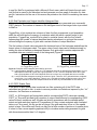
4.7.3 PSCF Output Matrices
PSCF matrices are printed as ASCII text files with the “.txt” extension. For further analysis by
GIS software, MetCor appends six-line header at the beginning of each PSCF matrix. The
coordinate system of the matrix is shown in Figure 8.
0, 90
359, 90
359, -90
0, -90
Figure 8: An example of a PSCF matrix with a 5x5 degree grid resolution and a spatial extent spanning the
world. Corner grid coordinates are shown. This is useful for reprojection in GIS software.
4.8 Additional Tools
MetCor includes optional tools to print histogram, scatter and elevation data along with PSCF
calculations. Elevation data can only be extracted from CMC formatted trajectories and is
printed as one simple tab-delimited text file per back trajectory. Histograms and scatter data
are also printed as simple, tab delimited text files easily readable by spreadsheet or data
processing software.
Options for using the following tools are found under the Utilities tab.
4.8.1 Elevation Plot Tool
If this option is selected, one text file per CMC-formatted back trajectory is printed as a tab
delimited text file containing only two columns: the forecast date and an associated elevation.
If a CMC-formatted file contains more than one elevation, multiple elevations are still plotted
4.0 – Basic Operation
Page 13
in one file. MetCor is packaged with a Microsoft Excel macro which will iterate through each
text file that is saved by the elevation tool and generate one line graph of elevation vs. date
per file. Instructions for the use of this macro are printed on the excel file containing the macro
itself.
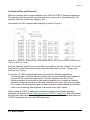
4.8.2 Grid Population and Unique Identifier Histogram Data
If this option is selected, two files containing histogram data are generated upon successful
PSCF analysis. The number of classes in the histogram must be an integer value in provided
to MetCor.
TaggedFreq_nij.txt contains two columns of data: the first corresponds to grid population
while the second lists the frequency of endpoints which fall within a certain range of grid
population. TaggedFreq_sourceID.txt is saved in a similar format, with the first column
representing the number of unique identifiers/starting elevations in a grid and the second
column listing the frequency of grids with a certain number of unique identifiers.
The first column of each value represents the horizontal axis of the histogram and defines the
lowest value of a histogram class. The upper value of each class can be obtained simply by
adding the interval between subsequent classes. Only grids which contain endpoints with
correlated data are counted in each of the histograms (Figure 9).
1
1772
1
1977
3
469
3
23
…
…
…
…
58
610
18
1
(a) TaggedFreq_nij.txt
(b) TaggedFreq_sourceID.txt
Figure 9: Examples of the histogram which MetCor prints out.
(a) A grid population histogram. There are 1772 endpoints which fall in grids with a grid population of 1 to 2,
469 endpoints which fall in grids with a grid population of 3 to 4, and 610 endpoints which fall in grids
with a grid population of 58 to 59. Endpoints which do not have any correlated data are not counted.
(b) A unique identifier histogram counting the number of grids. There are 1977 grids which have endpoints
coming from 1 to 2 unique identifiers. There is only 1 grid which contains endpoints coming from 18 to
19 unique identifiers. Grids with endpoints which do not have any correlated data are not counted.
4.8.3 PSCF Scatter Data
If the option to print scatter data is selected, two files containing all of the PSCF data
calculated are printed to disk. In order to remove possible size limitations imposed by the “.txt”
extension, the files have no extension.
PSCF_vs_NIJ lists each grid’s population and its corresponding PSCF values per variable.
PSCF_vs_SourceID lists each grid’s number of unique identifiers and its corresponding PSCF
values for each variable as well. All grids are listed in accordance with the defined spatial
extent and grid resolution (section 4.6) regardless of if they contain endpoints with correlated
data or not. As a result, the file can be very large if the grid resolution is fine or if the spatial
extent is large. Since Microsoft Excel can only plot a finite number of points on its scatter plots,
it is best to use a more capable graphical utility to visualize scatter data generated for grids
with dimensions smaller than 2 x 2 degrees.
4.0 – Basic Operation
Page 14
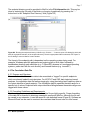
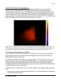
4.8.4 GNUPlot Script for Quick Visualization
For Linux based systems with GNUPlot installed and accessible from a command-line
interface, MetCor is bundled with an executable bash script for generating heat-map
representations of PSCF matrices. The bash script is executed from the command line and
must be placed in the folder containing the PSCF matrices. The header lines (section 4.7.4)
must be removed from each of the PSCF matrix files. A heat-map in the form of a portablenetwork graphics (*.png) formatted image is generated for each of the PSCF matrix files in the
folder. An example of such a heat-map is shown in Figure 10 below.
Figure 10: A visual representation of a PSCF matrix generated by MetCor’s bundled GNUPlot bash script. This
is useful for a quick analysis of the contents of a given PSCF matrix. The y-axis represents latitude while the xaxis represents longitude. The layout format and coordinate system is the same as that in section 4.7.3.
4.9 Running and Stopping Jobs on MetCor
A job on MetCor can be started by clicking the “RUN” button once all user-input has been
appropriately provided. Error message boxes will appear if any user-input is found to be
inadmissible or in the wrong format.
To interrupt a calculation, the MetCor must be terminated. This can be done by closing the
MetCor window or by the menu option File Exit. If MetCor is interrupted during any file
writing process such as printing histogram data or PSCF matrices, the output folder will
contain incomplete files. The output directory or files will not be rolled back to a previous state
or deleted. This must be done manually.
Multiple instances of MetCor can run on the same computer if the following requirements are
met:
- there can be no common output directory (section 4.2, 4.3) shared between the instances
of MetCor which are running
4.0 – Basic Operation
Page 15
-
sufficient physical memory required by all the instances of MetCor must be available
4.0 – Basic Operation
Page 16
5.0 Advanced Tools
Advanced tools available in MetCor include the use of configuration files for quick form
loading and use of the program’s backend for programming purposes. Configuration files are
useful if the same parameters are entered into MetCor multiple times, whereas the MetCor’s
backend is useful for users with programming knowledge who require more customization.
5.1 Using Configuration (*.cfg) Files
Configuration files are simple text files containing labelled parameters specific to MetCor.
5.1.1 Syntax and Format
The configuration file should be written and saved as a plain text file with the “cfg” extension.
MetCor recognizes lines of text beginning with ‘#’ as a comment. The general syntax for
setting all parameters except PSCF weights is:
<Parameter-Name>=<Value>
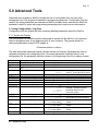
The table below lists parameter names, allowed values and formats. All parameters may be
optionally included in the configuration file. If the same parameter is defined twice in one
configuration file, the parameter definition closest to the beginning of the file is always chosen.
Name
Format
Description
Endpoint Directory
Output Directory
Full path of Correlated Data
File
Trajectory Format
Correct
Hours
totalLon
totalLat
dX
dY
ThreshType
Time Zone Correction in Hours
Trajectory Interval in Hours
Spatial extent in Longitude
Spatial extent in Latitude
Grid Resolution (longitude)
Grid Resolution (latitude)
Set thresholds
<Integer Value>
<Integer Value>
<Integer Value>
<Integer Value>
<Floating Point Value>
<Floating Point Value>
Percentile
TagType
Percentile setting (if applicable)
Domain of weighting function
<Floating Point Value>
ELEV
Elevation Plot Tool
SCAT
Print Scatter Data to Disk
HIST
Print Histograms to Disk
HistClasses
Number of Histogram Classes
EP
OP
IP
5.0 – Advanced Tools
Values
<Any File Path>
<Any File Path>
<Any File Path>
CMC
HYSPLIT
Avg
AvgSD
InFile
Percentile
NIJ
SourceID
ON
OFF or <Any Value>
ON
OFF or <Any Value>
ON
OFF or <Any Value>
<Integer Value>
-
read CMC Format
st
read 21 century HYSPLIT format
any value from -12 to 12
any value greater than 0
any value from 1 to 360
any value from 1 to 180
any value greater than 0.0
any value greater than 0.0
average
average + standard deviation
thresholds defined in file
percentile method
any value from 1.0 to 100.0
use grid population
use number of unique identifiers
enable
disable
enable
disable
enable
disable
any value greater than 0
Page 17
A PSCF weight table can also be entered into MetCor by writing “WEIGHT:” on one line and writing
values which must be separated by tabs. An example is shown below:
WEIGHT:
1
21
22
100
101 204
205 205
0.5
0.75
0.85
0.95
In the same way as the weighting table in the GUI (section 4.7.2), the first and second column
represent lower and upper bounds for either the grid population or number of unique
identifiers, respectively. The third column represents the weighting to apply.
5.1.2 Loading a *.cfg File on MetCor
To load a configuration file, select File Load Configuration to use a dialog box and select
the configuration file. Once opened, information from the configuration file is loaded onto the
form. The calculation must be started manually by the user by clicking “RUN” (section 4.9).
5.0 – Advanced Tools
Page 18
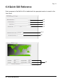
6.0 Quick GUI Reference
Each component of the MetCor GUI is labelled with the appropriate section to consult in this
User Guide.
4.2
4.3
4.4
4.2
4.3.3
4.5
4.6
6.0 – Quick GUI Reference
Page 19
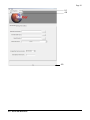
4.7.2
4.7.2
4.7.1
4.8.1
4.8.3
4.8.2
6.0 – Quick GUI Reference
Page 20
5.1
4.9
4.9
6.0 – Quick GUI Reference
Page 21
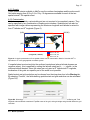
7.0 Examples
By the appropriate use of the correlated data file, PSCF matrices generated by MetCor can
represent many types of data. In one application, low resolution grids can be used to map
pollution data across the world. In another application, very high resolution grids can be used
to plot individual endpoints.
Some of the files used in the examples below are available in MetCor’s installation directory.
See the README file for more details.
7.1 Mapping Pollution Data
This is the most common application of MetCor. Meteorological data is received as HYSPLIT
or CMC formatted trajectories. On the basis of the date and time ranges specified in the
correlated data file, endpoints are appropriately tagged. PSCF matrices are then calculated
using pre-defined threshold values specific to the concentrations in the data file.
In this example, an analysis of PSCFs of “Pollutant-1” and “Pollutant-2” with CMC-formatted
back trajectories is conducted. The identifiers of the CMC-formatted back trajectories span
the dates of May 1, 2008 to June 1, 2008. The contents of the correlated data file
example_7_1.txt are shown below:
IDATE
20080501
20080507
20080514
20080531
ITIME
1305
1353
0600
1330
FDATE
20080507
20080513
20080514
20080601
FTIME
1313
1822
2359
1153
Pollutant_1
12.33
8.79
12.70
30.76
Pollutant_2
130.53
76.98
74.11
130.64
Rather than defining thresholds in the correlated data file, the “Average” method has been
chosen in the PSCF calculations. The following parameters are also used in the PSCF
calculations:
-
-
spatial extent: Northern Hemisphere
grid resolution: square grids, 1 deg. by 1 deg. Higher grid resolutions would prevent
endpoints from being pooled together effectively, whereas lower grid resolutions
overcompensate for errors in the back trajectories.
weighting scheme: none; the weighting table is left empty
threshold method: average
time-zone correction: +6 hours is chosen here because the back trajectory time zone is
offset by 6 hours from the times defined in the correlated data file.
additional plots to generate: scatter data and histogram data are plotted
7.0 – Examples
Page 22
7.2 Plotting Individual Trajectories
By using dummy variables in the correlated data file and a fine enough resolution to
discriminate between endpoints, PSCF matrices can represent plots of trajectories.
Suppose a series of CMC or HYSPLIT formatted trajectories are loaded onto MetCor
spanning May 1, 2008 to May 1, 2010. To plot only those trajectories for the months of May,
the correlated data file example_7_2.txt contains the following:
IDATE
20080501
20090501
20100501
THRESH
ITIME
0000
0000
0000
FDATE
20080531
20100531
20100531
FTIME
1800
1800
1800
X
1
1
1
0.5
The variable “X” has no meaning: it is simply used to tag endpoints of trajectories for selected
date ranges. By setting the threshold value lower than those used to tag endpoints, PSCF
values other than the no-data value (-1) represent a region of a grid containing endpoints of
interest.
The following parameters are also used in the PSCF calculations:
- spatial extent: Northern Hemisphere
- grid resolution: User-defined square grids, 0.1 deg. by 0.1 deg. The high resolution of the
grids ensures that one grid represents one endpoint.
- weighting scheme: an unweighted calculation would be required in this scenario. This
way, each grid which contains a back trajectory endpoint is flagged and gets a PSCF
value of 1
- threshold method: the thresholds are defined in the correlated data file
- time-zone correction: the times specified in the file are in the same time zone as the
trajectories. Therefore, the time-zone correction is option is set to “No Correction”
- additional data: no other plots are selected
7.0 – Examples
Page 23
8.0 Troubleshooting
8.1 Form Input Errors
Before starting any calculation, MetCor checks the data which has been entered in the
MetCor’s textboxes, tables and buttons. Commonly, some of the parameters required for a
successful calculation are not entered by the user or are provided in the wrong format. When
a calculation attempt is started by the user and such errors are encountered, an error
message will appear with details of the problem. The following table shows the error
messages which may appear and solutions:
Error Messages
Solution
--The Endpoint Files Directory has not been specified.
--The Correlated Data File has not been specified.
--The Output Directory has not been specified.
The form fields for these have been
left empty. Provide directories or
paths for the endpoints, correlated
data file and output directory
--The Output Directory could not be created.
The destination where the output
folder is stored may be read only.
Try specifying the output directory
in another destination.
--The Endpoint Files Directory does not exist.
--The Correlated Data File does not exist.
These paths and/or directories do not
exist. Specify valid directories and paths
only.
Choose CMC or HYSPLIT formatted
trajectories from the drop down box
under the File Information tab
Enter an integer-valued back trajectory
interval, in hours.
--A back trajectory format is not specified
--The Back trajectory interval is not specified.
--The Back trajectory interval specified is a zero or noninteger value.
--Grid Dimensions and Details are not specified.
--Grid Dimensions or Sizes are non-floating point or integer
values
--The Grid height and/or width are too small
Enter a valid spatial extent and nonzero floating point values for the fields
under the Binning tab.
--Threshold data values are not specified
Choose a method of determining
thresholds under the PSCF tab
--Percentile data is an inappropriate value
--Lower and/or Upper Bound Data contain non-integer
data.
If the percentile method has been
chosen as thresholds, enter a percentvalue for the percentile between 0 and
100.
Enter appropriate floating-point weights
in the weighting table under the PSCF
tab.
Enter integer values for the lower and
upper bounds only.
--The number of histogram bins specified is a noninteger value or has not been specified.
--The histogram class must be at least 1.
Enter an integer value for the number of
histogram classes of at least 1 if the
histogram option has been chosen.
--PSCF Weighting Factors Contain Non-Floating Point
Data
8.0 – Troubleshooting
Page 24
8.2 Errors During Calculations
Errors experienced while calculations are running care usually caused by inconsistencies in
the data which MetCor is analyzing. MetCor will terminate the calculation when such errors
are encountered. Changes made to the output directory will not be rolled back and must be
manually deleted by the user. The following table shows the error messages which may
appear during calculations and possible solutions:
Error Messages
Solution
Input File is not formatted Correctly
The format of the correlated data file is incorrect. Check to
make sure that the proper formatting guidelines (section
4.3.2) are followed.
Ensure that only trajectory files exist in the endpoint files
directory and that all of the trajectory files follow their
respective formatting guidelines (section 4.2)
MetCor could not load endpoints from disk.
Check to make sure that the directory is
valid and that back trajectories are
formatted correctly.
Runtime Error in Reading Input File.
Ensure that it is formatted correctly.
PSCF Matrix File IO Error.
This usually occurs because the times specified in the
input file are in the wrong format. Ensure that they are 4
digits in length
Check to make sure that the files in the output directory is
not in use. This may also occur if the output directory is
made read only.
8.3 Premature Termination
MetCor will unexpectedly terminate a calculation when computer hardware experiences
failures or if it resources are too limited. These insufficiencies include but are not limited to
low hard disk space or low available memory. MetCor does not explicitly notify users of such
errors, yet they often occur if the progress bar reads “Finished” without showing one or any of
the steps mentioned in section 4.1. Premature termination will often result in failure to
generate any output matrices or additional data. A possible list of solutions to hardware
insufficiencies is shown below:
Cause of Premature Termination
Solution
Not enough memory to complete a given MetCor
calculation.
-
-
Not enough free disk space to generate output
8.0 – Troubleshooting
-
close any programs which might be open in order to
free more memory; restart MetCor once this is done
(for Windows-based operating systems only)
the grid resolution might be too high; use a lower grid
resolution*
lower the number of variables in the correlation data
file: or split the variables between two or more
correlation data files and run those calculations
separately
manually allocate more memory to the instance of
MetCor (Unix-based operating systems only)
Free disk space
Direct output to a directory of a different drive or
partition.