Download HYDROSIM User's Guide - Groupe GRE-EHN

HYDROSIM
User’s Guide
HYDROSIM version 1.0a06
June 2000
Copyright  1999-2000 INRS
Table of contents
Chapter 1 Overview of the software__________________________________________________ 1-1
Uses of the software _____________________________________________________________________ 1-1
Material requirements ____________________________________________________________________ 1-1
User’s licence __________________________________________________________________________ 1-2
Launching the software ___________________________________________________________________ 1-2
Language ______________________________________________________________________________ 1-3
physical measurements units _______________________________________________________________ 1-3
Stopping the software ____________________________________________________________________ 1-3
Chapter 2 Work pocedure__________________________________________________________ 2-1
Schematic description ____________________________________________________________________ 2-1
Structure of the command file ______________________________________________________________ 2-1
Definition____________________________________________________________________________ 2-1
Blocks ______________________________________________________________________________ 2-3
COND ____________________________________________________________________________ 2-4
COOR ____________________________________________________________________________ 2-4
ELEM ____________________________________________________________________________ 2-4
ERR ______________________________________________________________________________ 2-5
FCRT _____________________________________________________________________________ 2-5
FIN ______________________________________________________________________________ 2-5
FORM ____________________________________________________________________________ 2-6
INIT(real,real,...,real) ________________________________________________________________ 2-6
PRCO_____________________________________________________________________________ 2-6
PREL _____________________________________________________________________________ 2-7
PRGL(real,real,...,real) _______________________________________________________________ 2-7
PRNO ____________________________________________________________________________ 2-7
POST _____________________________________________________________________________ 2-8
RESI _____________________________________________________________________________ 2-8
SOLC_____________________________________________________________________________ 2-8
SOLR_____________________________________________________________________________ 2-9
SOLV(real,real,real) _________________________________________________________________ 2-9
STOP _____________________________________________________________________________ 2-9
Variables ___________________________________________________________________________ 2-10
Type - string of characters____________________________________________________________ 2-10
ELTYP___________________________________________________________________________ 2-11
FFFIN ___________________________________________________________________________ 2-11
FFINI ____________________________________________________________________________ 2-11
MCND ___________________________________________________________________________ 2-11
MCOR ___________________________________________________________________________ 2-11
MELE ___________________________________________________________________________ 2-11
MERR ___________________________________________________________________________ 2-11
MEXE ___________________________________________________________________________ 2-12
MFCR ___________________________________________________________________________ 2-12
MFIL ____________________________________________________________________________ 2-12
MFIN ____________________________________________________________________________ 2-12
MINI ____________________________________________________________________________ 2-12
MPRE ___________________________________________________________________________ 2-12
MPRN ___________________________________________________________________________ 2-12
MPST____________________________________________________________________________ 2-12
MRES ___________________________________________________________________________ 2-12
MSLC ___________________________________________________________________________ 2-13
MSLR ___________________________________________________________________________ 2-13
I
STEMP __________________________________________________________________________ 2-13
Type - integer _____________________________________________________________________ 2-13
ILU _____________________________________________________________________________ 2-13
IMPR ____________________________________________________________________________ 2-13
NITER ___________________________________________________________________________ 2-14
NPAS____________________________________________________________________________ 2-14
NPREC __________________________________________________________________________ 2-14
NRDEM__________________________________________________________________________ 2-14
Type - real ________________________________________________________________________ 2-14
ALFA ___________________________________________________________________________ 2-15
DELPRT _________________________________________________________________________ 2-15
DPAS____________________________________________________________________________ 2-15
EPSDL___________________________________________________________________________ 2-15
OMEGA _________________________________________________________________________ 2-15
TASCND _________________________________________________________________________ 2-15
TASINI __________________________________________________________________________ 2-15
TASPRE _________________________________________________________________________ 2-15
TASPRN _________________________________________________________________________ 2-16
TASSLC _________________________________________________________________________ 2-16
TASSLR _________________________________________________________________________ 2-16
TINI _____________________________________________________________________________ 2-16
Structure of file names___________________________________________________________________ 2-16
Progress of the simulation ________________________________________________________________ 2-17
Definition___________________________________________________________________________ 2-17
Work load __________________________________________________________________________ 2-17
End message ________________________________________________________________________ 2-17
Chapter 3 How to manage a simulation ? _____________________________________________ 3-1
Create a new simulation __________________________________________________________________ 3-1
Define the discretization of the problem ______________________________________________________ 3-1
Read the data ___________________________________________________________________________ 3-2
Read the coordinates ___________________________________________________________________ 3-2
Read the connectivities _________________________________________________________________ 3-3
Read the global properties _______________________________________________________________ 3-3
Read the nodal properties _______________________________________________________________ 3-3
Read the elementary properties ___________________________________________________________ 3-4
Read the initial solution_________________________________________________________________ 3-4
Read the boundary conditions ____________________________________________________________ 3-5
Read the concentrated solicitations ________________________________________________________ 3-6
Read the distributed solicitations__________________________________________________________ 3-6
Solve the problem _______________________________________________________________________ 3-7
Print the results _________________________________________________________________________ 3-8
Print the degrees of freedom _____________________________________________________________ 3-8
Print the estimate of the numerical errors ___________________________________________________ 3-9
Print the post-processing ________________________________________________________________ 3-9
Print the residuals ____________________________________________________________________ 3-10
Print the function current_______________________________________________________________ 3-10
Chapter 4 How to obtain a hydrodynamic solution? ____________________________________ 4-1
How to validate the input data (preliminary phase)?_____________________________________________ 4-1
How to give the model an initial run? ________________________________________________________ 4-2
Scenarios of boundary conditions _________________________________________________________ 4-2
Closed boundary ____________________________________________________________________ 4-2
Open boundary _____________________________________________________________________ 4-3
Scenarios of initial conditions ____________________________________________________________ 4-4
Static solution (static water body) _______________________________________________________ 4-4
II
Quasi linear solution _________________________________________________________________ 4-4
Improved quasi-linear solution _________________________________________________________ 4-5
Reference solution ___________________________________________________________________ 4-5
How to converge the solution? _____________________________________________________________ 4-6
Solution method ______________________________________________________________________ 4-6
GMRES solution algorithm____________________________________________________________ 4-6
Preconditioning matrix _______________________________________________________________ 4-8
Memory space ______________________________________________________________________ 4-8
Precision __________________________________________________________________________ 4-9
Solution update _______________________________________________________________________ 4-9
Relax the solution update ____________________________________________________________ 4-10
Limit the solution update_____________________________________________________________ 4-10
Behaviour of the solver ________________________________________________________________ 4-10
Has convergence been reached? _________________________________________________________ 4-12
Advanced solution strategies____________________________________________________________ 4-13
Driven by the downstream water level __________________________________________________ 4-13
Driven by the connective acceleration (inertia)____________________________________________ 4-15
Driven by the upper bound of viscosity _________________________________________________ 4-16
Driven by the time step ______________________________________________________________ 4-18
Practical advice ______________________________________________________________________ 4-19
How to validate the model?_______________________________________________________________ 4-20
Control of mass balance _______________________________________________________________ 4-21
Control of Drying/Wetting _____________________________________________________________ 4-21
How to adjust the model (calibration)? ______________________________________________________ 4-23
Calibrate by the discharge ______________________________________________________________ 4-23
Calibrate by the water level _____________________________________________________________ 4-24
Calibrate by velocities _________________________________________________________________ 4-24
Frequently asked questions _______________________________________________________________ 4-25
How to evaluate the turbulent viscosity?___________________________________________________ 4-25
How to minimize the level of error? ______________________________________________________ 4-26
Has the solution diverge? ______________________________________________________________ 4-26
What is numerical viscosity?____________________________________________________________ 4-26
What is the role of the upper bound of the viscosity? _________________________________________ 4-27
What are the effects of an excessive dissipation? ____________________________________________ 4-27
How to estimate the discharge transiting in the domain? ______________________________________ 4-27
Chapter 5 Appendix_______________________________________________________________ 5-1
Language dictionary _____________________________________________________________________ 5-1
HYDROSIM in English ________________________________________________________________ 5-1
HYDROSIM in Spanish ________________________________________________________________ 5-1
HYDROSIM in French _________________________________________________________________ 5-2
Library of finite elements _________________________________________________________________ 5-2
Finite element SVC ______________________________________________________________________ 5-2
How to reach it? ____________________________________________________________________ 5-2
Function___________________________________________________________________________ 5-2
Properties__________________________________________________________________________ 5-3
Boundary conditions _________________________________________________________________ 5-4
Solicitations ________________________________________________________________________ 5-5
Initial solution ______________________________________________________________________ 5-5
Finite element SVCRNM _________________________________________________________________ 5-6
How to reach it? ____________________________________________________________________ 5-6
Function___________________________________________________________________________ 5-6
Properties__________________________________________________________________________ 5-6
Boundary conditions _________________________________________________________________ 5-7
Solicitations ________________________________________________________________________ 5-8
III
Initial solution ______________________________________________________________________ 5-9
Library of temporal schemes ______________________________________________________________ 5-10
EULER ____________________________________________________________________________ 5-10
STATIQ____________________________________________________________________________ 5-10
Processing of transient data _______________________________________________________________ 5-10
Block dependencies_____________________________________________________________________ 5-11
Dependencies between blocks___________________________________________________________ 5-11
Dependencies blocks-variables __________________________________________________________ 5-12
Dependencies blocks-strings of characters _______________________________________________ 5-12
Dependencies blocks-integer variables __________________________________________________ 5-13
Dependencies of blocks-real variables __________________________________________________ 5-13
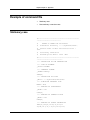
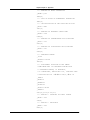
Example of command file ________________________________________________________________ 5-14
Stationary case_______________________________________________________________________ 5-14
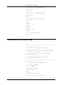
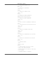
Non-stationary or transient case _________________________________________________________ 5-16
Formats of input files ___________________________________________________________________ 5-19
Boundary conditions file _______________________________________________________________ 5-19
Connectivities file ____________________________________________________________________ 5-20
Coordinates file ______________________________________________________________________ 5-21
Elementary properties file ______________________________________________________________ 5-22
Nodal properties file __________________________________________________________________ 5-22
Solicitations file______________________________________________________________________ 5-24
Initial solution file ____________________________________________________________________ 5-25
Formats of results files __________________________________________________________________ 5-26
Degrees of freedom file ________________________________________________________________ 5-27
Numerical errors file __________________________________________________________________ 5-28
Post-processing file ___________________________________________________________________ 5-28
Residuals file ________________________________________________________________________ 5-29
Function current file __________________________________________________________________ 5-30
Chapter 6 Glossary _______________________________________________________________ 6-1
IV
HYDROSIM - User’s Guide
HYDROSIM - User’s Guide
The HYDROSIM manual provides all the information needed to
use the software. HYDROSIM is essentially a numerical driver
deprived of any graphic interface. It functions only in text mode.
The main sections of the manual are :
HYDROSIM 1.0a06 - User's Guide
•
Overview of the software
•
Work procedure
•
How to manage a simulation ?
•
How to obtain a hydrodynamic solution?
•
Appendix
Chapter Chapter 1 : Overview of the software
Chapter 1 Overview of the software
•
Uses of the software ;
•
Material requirements ;
•
User’s licence ;
•
Launching the software ;
•
Language ;
•
Physical measurements units ;
•
Stopping the software.
Uses of the software
HYDROSIM is a code Finite Elements designed and developed
by { XE "éléments finis" }INRS-Eau, a research center part of
Université du Québec, to provide a tool for horizontal twodimensional simulation of the hydrodynamics of estuaries, rivers
and streams. It can be useful to researchers from various fields
of interest, but requires some notion of fluvial hydraulics.
The program is based on the solution of the { XE "éléments finis"
}Saint-Venant equations by Finite elements{ XE "Saint-Venant" },
in steady or non steady flow regime, governing the
hydrodynamics of streams. HYDROSIM also permits the
simulation of drying/wetting conditions on shores and beaches,
using a new method developed by scientists at INRS-Eau.
Material requirements
HYDROSIM runs on a personal computer (PC) on the Win32
platforms (Windows 95/98, Windows NT3.51/4.0 etc...){ XE
"plateforme :Win32" } and dynamically manages the memory it
requires.{ XE "mémoire" } For optimal performances and good
execution speed, it is recommended to run the software in
Random Access memory (RAM) rather than on disk memory
which considerably reduces execution speed.
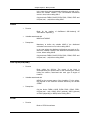
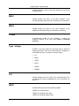
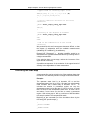
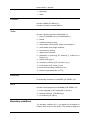
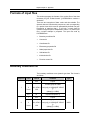
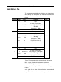
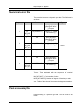
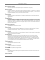
The memory needed depends directly on the size of the
application to be simulated. The index used to determine the size
of a simulation in Megabytes{ XE "mégabytes" } is the total
number of degrees of freedom (TNDF{ XE "NDLT" }). For the
solution parameters advocated, the memory allocated by
HYDROSIM is estimated at bout 6.5x10-4 times TNDF{ XE
"NDLT" } in Megabytes{ XE "mégabytes" }. As an indicative,
HYDROSIM 1.0a06 - User's Guide
1-1
Chapter Chapter 1 : Overview of the software
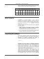
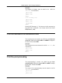
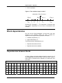
Table 1 presents the memory required for TNDF values ranging
from{ XE "mémoire" } { XE "NDLT" }10 000 to 100 000.
Table 1 : Memory required for various TNDF values.
TNDF
10
20
30
40
50
60
70
80
90
100
6.5
13
19.5
26
32.5
39
45.5
52
58.5
65
(x1000)
Memory
(Meg)
User’s licence
HYDROSIM is a protected software. To use it after the
installation, it is necessary to register the software according to
the procedure described in the file{ XE "licence :enregistrement"
} hydrosim_enregistrement.txt available in the same
directory as hydrosim.exe.
Following registration, one of two (02) types of licence is granted{
XE "licence :type" }:
1 - DEMO : granted for demonstration exercises. Access to
certain functionalities of the software is unauthorized. In fact,
calculations and printing of results are not possible.
2 - FULL : gives access to all the functionalities of the software.
Duration of the licence may be limited or unlimited.
Launching the software
On the Win32 platforms (Windows 95/98, Windows NT3.51/4.0
etc...),{ XE "plateforme :Win32" } the launching of the software is
activated in a window in MS-DOS text mode{ XE
"exécution :démarrage" } (command prompt), by typing :
hydrosim
Immediately after being launched, HYDROSIM systematically
displays the name of the software. Then, it displays the date, the
time and the memory space used. Finally, the information on the
software licence are displayed : name of the software{ XE
"licence :nom du logiciel" }, access code and type of licence{ XE
"licence :code d’accès" }{ XE "licence :type" }.
These information can be displayed either at the prompt or in an
output file{ XE "fichier:sortie" }. The software reads the
instructions of the fortran number 5 unit and prints the information
relative to the progress of the simulation in the fortran number 6.
The input/output fortran units 5 and 6 can be redirected
1-2
HYDROSIM 1.0a06 - User's Guide
Chapter Chapter 1 : Overview of the software
respectively to the command file fichier.inp and to the output
file as follows:
hydrosim < fichier.inp > fichier.out
If no input/output files are specified, execution will occur at the
prompt. In this case, all the output messages are displayed
directly on the screen. Also, immediately after launching, the
software is in a scanning mode, which can be deactivated by
typing the command{ XE "mode balayage" } STOP.
In the case when the execution is managed by a command file,
the scanning mode is automatically deactivated.
The output messages of HYDROSIM are displayed in an output
file, if it has previously been specified.
Language
HYDROSIM has a language translation module which translates
the internal messages of the software. The language of use is
defined in the configuration file{ XE "langue" } hydrosim.ini{
XE "fichier:configuration" } using the variable LANGUE. The
syntax{ XE "syntaxe :langue" } is as follows :
_LANGUE=’.xxx’
The characters xxx define the language of use (see Language
dictionary). French is the default language.
Physical measurements units
In HYDROSIM, physical measurements are expressed in the
International System (IS) units.
Stopping the software
For an execution without input files{ XE "fichier:entrée" }, a two-step procedure is
followed to stop the software. First, you must exit the scanning mode by typing the
command STOP followed by Enter. The same operation is repeated to stop the
software.
HYDROSIM 1.0a06 - User's Guide
1-3
Chapter Chapter 2 : Work procedure
Chapter 2 Work procedure
HYDROSIM is a modular software, where each module is
dedicated to a specific task. The objective of this chapter on the
work procedure is to present all the modules found in
HYDROSIM, their function, as well as the prerequisite and
dependencies related to their execution. The sections in this
chapter address the following items :
•
Schematic description
•
Structure of the command file
•
Structure of file names
•
Progress of the simulation
Schematic description
After launching HYDROSIM, the simulation consists in having the
different modules work together to reach the overall objective.
The different tasks can be achieved using a series of commands.
Schematically, the commands can be classified in three groups :
•
input data read commands
•
solution commands
•
output result printing commands
Structure of the command file
•
Definition
•
Blocks
•
Variables
Definition
The command file comprises instructions and optional
commentaries allowing to customize each simulation. The
commentaries may be preceded by either one or the other
symbol # or !.
HYDROSIM 1.0a06 - User's Guide
2-1
Chapter Chapter 2 : Work procedure
All the commentaries preceded by # are automatically printed at
the output, which is not the case for those preceded by !.
The instructions are made of a series of commands consisting of
Blocks and Variables. The instructions which are systematically
found in the command file are the choice of the type of finite
element and of the temporal scheme, the definitions of the
formulation, data and result files, and calls for blocks to execute
specific tasks. Every simulation must be punctuated by the call to
the block STOP which ends the execution of HYDROSIM. Thus
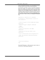
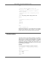
the command file reads as follows (see Example of command
file) :
# Specimen of command file for HYDROSIM
# Information or identifications relative to
# the simulation
! Choose the type of finite element(see ELTYP).
Instruction
! Choose the type of temporal scheme(see
! STEMP).
Instruction
! Define the formulation (see FORM)
Instruction
! Definition of data and results files.
Instruction
! List of instructions for the acquisition of
! data, the simulation and post-processing.
Instruction
.
.
.
! End of the simulation.
STOP
Remark{ XE "Remarque" } : Each instruction must be written on
only one line of 1024 characters maximum.
2-2
HYDROSIM 1.0a06 - User's Guide
Chapter Chapter 2 : Work procedure
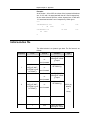
Blocks
Each command is identified by an execution block. Each block
has an optional printing unit which returns in output, in part or in
totality, the input data and/or information specific to each block.
The level of printing of the information is driven by the positive
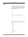
integer m which is equal to 0 by default. The syntax of blocks is{
XE "niveau :impression" } :
BLOCK
or
BLOCK[M]
Certain blocks are accompanied by a table of real values :
BLOCk(real,real,...,real)
or
BLOCK[M]( real,real,...,real)
The name of each block is a reserved word which must not
exceed 4 characters maximum. In HYDROSIM, there are 18
blocks :
HYDROSIM 1.0a06 - User's Guide
•
COND
•
COOR
•
ELEM
•
ERR
•
FCRT
•
FIN
•
FORM
•
INIT(real,real,...,real)
•
PRCO
•
PREL
2-3
Chapter Chapter 2 : Work procedure
•
PRGL(real,real,...,real)
•
PRNO
•
POST
•
RESI
•
SOLC
•
SOLR
•
SOLV(real,real,real)
•
STOP
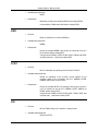
COND
•
Function
Block for reading the boundary CONDitions.
•
Variables associated with
MCND and TASCND
•
Prerequisite
Mandatory to define the variable MCND before calling COND.
Define the variable TASCND (=0 by default) if the boundary
conditions evolve in time, before calling COND.
Call the blocks COOR, ELEM, PRGL, PRNO, PREL and
INIT(real,real,...,real) before calling COND.
COOR
•
Function
Block for reading the mesh COORdinates.
•
Variable associated with
MCOR
•
Prerequisite
Mandatory to define the variable MCOR before calling COOR.
Call the block FORM before calling COOR.
ELEM
•
Function
Block for reading mesh ELEMents
2-4
HYDROSIM 1.0a06 - User's Guide
Chapter Chapter 2 : Work procedure
•
Variable associated with
MELE
•
Prerequisite
Mandatory to define the variable MELE before calling ELEM.
Call the blocks FORM and COOR before calling ELEM.
ERR
•
Function
Block of calculation of numerical ERRors.
•
Variable associated with
MERR
•
Prerequisite
Define the variable MERR if the printing of numerical errors in a
file is desired, before calling ERR.
Call the blocks FORM, COOR, ELEM, PRGL, PRNO and PREL
and INIT(real,real,...,real) before calling ERR.
FCRT
•
Function
Bloc of calculation and printing of the Function CuRrenT.
•
Variables associated with
MFCR for read/write of the function current, MEXE for the
progress status of the simulation and ILU, NRDEM, NITER,
OMEGA and EPSDL for the solution.
•
Prerequisite
Define the variable MFCR if the printing of the function current in
a file is desired as well as ILU, NRDEM, NITER, OMEGA et
EPSDL before calling FCRT.
Call the blocks FORM, COOR, ELEM, PRGL, PRNO, PREL and
INIT(real,real,...,real) before calling FCRT.
FIN
•
Function
Bloc of FINal printing of the solution in binary format.
•
Variables associated with
MFIN and FFFIN.
HYDROSIM 1.0a06 - User's Guide
2-5
Chapter Chapter 2 : Work procedure
•
Prerequisite
Define the MFIN, if printing of the solution in a file is desired
(strongly recommended), and FFFIN before calling FIN.
Call the blocks FORM, COOR, ELEM, PRGL, PRNO and PREL
and INIT(real,real,...,real) before calling FIN.
FORM
•
Function
Block of definition of the FORMulation of the problem. Must
imperatively be called at the beginning of each simulation.
•
Variables associated with
ELTYP and STEMP.
•
Prerequisite
Absolutely define the variables ELTYP and STEMP before calling
FORM.
Warning{ XE "Mise en garde" } : After calling FORM, all the data
in virtual memory are initialized.
INIT(real,real,...,real)
•
Function
Block of update of the INITial solution of the problem. The syntax
of the block is accompanied of an optional table of real containing
the initialization parameters associated with the type of finite
element (see Library of finite elements).
•
Variables associated with
MINI, FFINI and TASINI
•
Prerequisite
Define the variable MINI if the initial solution is stored on file
before calling INIT.
In the case where the initial solution must be read on a file :
define the variables FFINI and TASINI, if the initial solution
evolves in time, before calling INIT.
Call the blocks FORM, COOR, ELEM, PRGL, PRNO and PREL
before calling INIT.
PRCO
•
Function
Block of calculation of the pointers for a PReCOnditioning of the
type matrix ILU.
2-6
HYDROSIM 1.0a06 - User's Guide
Chapter Chapter 2 : Work procedure
•
Variables associated with
ILU and DELPRT.
•
Prerequisite
Call the blocks FORM, COOR and ELEM before calling PRCO.
PREL
•
Function
Block for reading the Elementary PRoperties.
•
Variables associated with
MPRE and TASPRE
•
Prerequisite
Define, depending on the type of finite element (see Library of
finite elements), the variable MPRE before calling PREL.
Define the variable TASPRE before calling PREL if the
elementary properties evolve in time.
Call the blocks FORM, COOR, ELEM, PRGL and PRNO before
calling PREL.
PRGL(real,real,...,real)
•
Function
Block for reading the Global PRoperties.
•
Variable associated with
None
•
Prerequisite
Call the block FORM before calling PRGL.
PRNO
•
Function
Block for reading the NOdal PRoperties.
•
Variables associated with
MPRN and TASPRN
•
Prerequisite
Define, depending on the type of finite element (see Library of
finite elements), the variable MPRN before calling PRNO.
HYDROSIM 1.0a06 - User's Guide
2-7
Chapter Chapter 2 : Work procedure
Define the variable TASPRN if the nodal properties evolve in
time, before calling PRNO.
Call the blocks FORM, COOR, ELEM and PRGL before calling
PRNO.
POST
•
Function
Block of POST-processing of the results.
•
Variable associated with
MPST
•
Prerequisite
Define the variable MPST before calling POST if printing of the
post-processing in a file is desired.
Call the blocks FORM, COOR, ELEM, PRGL, PRNO, PREL and
INIT(real,real,...,real) before calling POST.
RESI
•
Function
Block of calculation of the RESIduals.
•
Variable associated with
MRES
•
Prerequisite
The definition of the variable MRES before calling RESI is
mandatory if printing of the residuals in a file is desired.
Call the blocks FORM, COOR, ELEM, PRGL, PRNO, PREL,
INIT(real,real,...,real) and COND before calling RESI.
SOLC
•
Function
Block for reading the Concentrated
"sollicitations :concentrées" }.
•
SOLicitations{
XE
Variables associated with
MSLC and TASSLC
•
Prerequisite
Mandatory to define the variable MSLC if the concentrated
solicitations are stored on file, before calling SOLC.
2-8
HYDROSIM 1.0a06 - User's Guide
Chapter Chapter 2 : Work procedure
In the case where the concentrated solicitations are read on file :
define the variable TASSLC if the concentrated solicitations
evolve in time, before calling SOLC.
Call the blocks FORM, COOR, ELEM, PRGL, PRNO, PREL and
INIT(real,real,...,real) before calling SOLC.
SOLR
•
Function
Block for the reading of
"sollicitations :réparties" }.
•
distRibuted
SOLicitations{
XE
Variables associated with
MSLR and TASSLR
•
Prerequisite
Mandatory to define the variable MSLR if the distributed
solicitations are stored on file, before calling SOLR.
In the case where the distributed solicitations are read on file :
define the variable TASSLR if the distributed solicitations evolve
in time, before calling SOLR.
Call the blocks FORM, COOR, ELEM, PRGL, PRNO, PREL and
INIT(real,real,...,real) before calling SOLR.
SOLV(real,real,real)
•
Function
Block calling the SOLVer. The syntax of the block is
accompanied by an optional table of real containing the factors
limiting the solution, associated with each type of degree of
freedom.
•
Variables associated with
MEXE for the progress status of the simulation. For the others,
they depend on the resolution scheme defined by the variable
STEMP.
•
Prerequisite
Call the blocks FORM, COOR, ELEM, PRGL, PRNO, PREL,
INIT(real,real,...,real), COND, SOLC (optional), SOLR (optional)
et PRCO (depending on IMPR) before calling SOLV.
STOP
•
Function
Block to STOP the software.
HYDROSIM 1.0a06 - User's Guide
2-9
Chapter Chapter 2 : Work procedure
•
Variable associated with
None
•
Prerequisite
None.
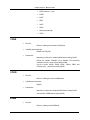
Variables
The variables are always followed by a dynamic field defining
them. The syntax of variables{ XE "syntaxe :variable" } is :
_VARIABLE=value
The dynamic field value comes in three forms :
•
Type - string of characters between single quotation marks (‘
‘).
•
Type - integer.
•
Type - real.
Type - string of characters
The variables of the type string of characters are generally used
to define the names of data and results files. Their use may be
optional or mandatory. In HYDROSIM, there are 19 variables of
the type string of characters :
2-10
•
ELTYP
•
FFFIN
•
FFINI
•
MCND
•
MCOR
•
MELE
•
MERR
•
MEXE
•
MFCR
•
MFIL
•
MFIN
HYDROSIM 1.0a06 - User's Guide
Chapter Chapter 2 : Work procedure
•
MINI
•
MPRE
•
MPRN
•
MPST
•
MRES
•
MSLC
•
MSLR
•
STEMP
ELTYP
A fundamental variable for any simulation. It defines the TYPe of
finite ELement to be used (see Library of finite elements).
FFFIN
Variable defining the format (ASCII or binary) of the degrees of
freedom file. It may have a ASCII ( default) or BIN value.
FFINI
Variable defining the format (ASCII or binary) of the initial
solution file. It may have a ASCII ( default) or BIN value.
MCND
Variable defining the name or the name extension of the
boundary CoNDitions file.
MCOR
Variable defining the name or the name extension of the mesh
nodes COoRdinates file.
MELE
Variable defining the name or the name extension of the
connectivities of the mesh ELEments file.
MERR
HYDROSIM 1.0a06 - User's Guide
2-11
Chapter Chapter 2 : Work procedure
Variable defining the name or the name extension of the results
of the numerical ERRors file.
MEXE
Variable defining the name or the name extension of the
progress monitoring of the simulation EXEcution file.
MFCR
Variable defining the name or the name extension of the
read/write of the Function CuRrent file.
MFIL
Variable defining the generic name or the directory of all the input
and output FILes.
MFIN
Variable defining the name or the name extension of the FINal
solution printing file.
MINI
Variable defining the name or the name extension of the INITial
solution file.
MPRE
Variable defining the name or the name extension of the
Elementary Properties file.
MPRN
Variable defining the name or the name extension of the Nodal
Properties file.
MPST
Variable defining the name or the name extension of the results
of PoSt-Processing file.
MRES
2-12
HYDROSIM 1.0a06 - User's Guide
Chapter Chapter 2 : Work procedure
Variable defining the name or the name extension of the results
of RESiduals file.
MSLC
Variable defining the name or the name extension of the
Concentrated SoLicitations file{ XE "sollicitations :concentrées" }.
MSLR
Variable defining the name or the name extension of the
distRibuted SoLicitations file{ XE "sollicitations :réparties" }.
STEMP
A fundamental variable for any simulation. It defines the
TEMPoral Scheme to be used. (see Library of temporal
schemes).
Type - integer
Variables of the type integer are generally used to define the
solution parameters. Their use is either optional or mandatory. In
HYDROSIM, there are 5 variables of the type integer :
•
ILU
•
IMPR
•
NITER
•
NPAS
•
NPREC
•
NRDEM
ILU
Variable defining the level of filling for a preconditioning of the
type matrix{ XE "niveau :remplissage ILU" } ILU. By default, it is
equal to 0.
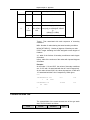
IMPR
Variable defining the type PReconditioning Matrix :
_IMPR=0 for indented matrix
_IMPR=1 for diagonal mass matrix
_IMPR=2 for diagonal tangent matrix
HYDROSIM 1.0a06 - User's Guide
2-13
Chapter Chapter 2 : Work procedure
_IMPR=3 for ILU matrix
By default, it is equal to 1.
NITER
Variable defining the Number of ITERations. By default, it is
equal to 25.
NPAS
Variable defining the Number of steps for the division of time t in
increment ∆t in the case of a transient or non stationary
simulation{ XE "transitoire" }. By default, it is equal to 1.
NPREC
Variable defining the Number of PREConditioning. By default, it
is equal to 1.
NRDEM
Variable defining the Number of Restarts. By default, it is equal to
25.
Type - real
Variables of the type « real » are used to define the parameters
of the solution method and the data in a non stationary context.
Their use is either optional or mandatory. In HYDROSIM, there re
12 variables of the type « real » :
2-14
•
ALFA
•
DELPRT
•
DPAS
•
EPSDL
•
OMEGA
•
TASCND
•
TASINI
•
TASPRE
•
TASPRN
•
TASSLC
•
TASSLR
HYDROSIM 1.0a06 - User's Guide
Chapter Chapter 2 : Work procedure
•
TINI
ALFA
Variable defining the coefficient α (ALFA) of the temporal scheme
EULER. It can take values between 0 and 1 inclusive. By default,
it is equal to 1.
DELPRT
Variable defining the coefficient ∆ (DELta) of disruption of the ILU
preconditioning matrix. By default, it is equal to 10-8.
DPAS
Variable defining the time step{ XE "pas de temps" } ∆t (Delta t)
for the discretization of the time. By default, it is equal to 10+12.
EPSDL
Variable defining the precision ε (EPSilon) of the Degrees of
freedom. By default, it is equal to 10-06.
OMEGA
Variable defining the factor ω (OMEGA) of relaxation of the
degrees of freedom. By default, it is equal to 1.
TASCND
Variable defining the Time ASsociated with the initial reading of
the non stationary boundary CoNDitions (see Processing of
transient data ).
TASINI
Variable defining the Time ASsociated with the initial reading of
the non stationary INItial solution (see Processing of transient
data ).
TASPRE
Variable defining the Time ASsociated with the initial reading of
the non stationary Elementary PRoperties (see Processing of
transient data ).
HYDROSIM 1.0a06 - User's Guide
2-15
Chapter Chapter 2 : Work procedure
TASPRN
Variable defining the Time ASsociated with the initial reading of
the non stationary Nodal PRoperties (see Processing of
transient data ).
TASSLC
Variable defining the Time ASsociated with the initial reading of
the non stationary Concentrated SoLicitations (see Processing
of transient data ).
TASSLR
Variable defining the Time ASsociated with the initial reading of
the
non
stationary
distRibuted
SoLicitations{
XE
"sollicitations :réparties" } (see Processing of transient data ).
TINI
Variable defining the INItial Time of the simulation.
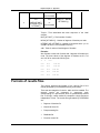
Structure of file names
The names of the HYDROSIM data and results files are
systematically defined by the concatenation of the values of two
Variables of the Type - string of characters. In the order, the first
common to all files is MFIL and the second is associated with the
appropriate block (see Blocks).
Example :
The name of the file associated with block XXX accepting MXXX
as variable of the type string of characters, is determined by one
or the other of the two following procedures :
_MFIL=’name1’
_MXXX=’name2’
or
_MFIL=’’
_MXXX=’name1name2’
In both cases, the file name resulting from the association of, in
the order, MFIL and MXXX is name1name2.
Remark{ XE "Remarque" } : The maximum length of file names
cannot exceed 217 characters.
2-16
HYDROSIM 1.0a06 - User's Guide
Chapter Chapter 2 : Work procedure
Progress of the simulation
•
Definition
•
Work load
•
End message
Definition
The progress of the simulation is accessible on the simulation
monitoring file defined by the variable MEXE (see Structure of file
names).
Typically, when a simulation is running, there is only one line of
message containing an integer comprised between 1 and 100 in
the simulation monitoring file. It expresses, in percentage (%) of
the Work load, the state of progress of the problem solving
procedure.{ XE "exécution :avancement" }
Work load
The work load is an integer equal to the maximum number of
iterations possible{ XE "exécution :volume" }. It is automatically
calculated during the scanning mode. It is then displayed at the
prompt or in the output file (see Launching the software) when
the scanning mode is exited.
End message
At the end of the HYDROSIM simulation, the following message
appears systematically in the simulation monitoring file{ XE
"fichier:suivi de la simulation" } :
100
END
In the output file or at the prompt, the date and time of the end of
the simulation are displayed, as well as the total duration. The
memory space used is also given.
Remark{ XE "Remarque" } : The duration of the same simulation
may vary if the work conditions are modified.
HYDROSIM 1.0a06 - User's Guide
2-17
Chapter Chapter 2 : Work procedure
2-18
HYDROSIM 1.0a06 - User's Guide
Chapter Chapter 3 : How to manage a simulation ?
Chapter 3 How to manage a simulation ?
The objective of this chapter is to present the procedure to build
a command file{ XE "fichier:commandes" } (see Structure of the
command file) from the Variables and Blocks, to manage a
simulation. At each step, the variable to define and the block to
call are indicated. To make sure that the rules of dependencies
between blocks and variables are respected (see Block
dependencies), it is recommended to follow the procedure
below :
•
Create a new simulation
•
Define the discretization of the problem
•
Read the data
•
Solve the problem
•
Print the results
Create a new simulation
When creating a new simulation, it is recommended (although
optional) to insert in the command file, text (a maximum of 1024
per line) to identify the physical process to be simulated. It
consists mainly in indicating the origin of the terrain data, the
choice of boundary conditions, of solicitations and of initial
conditions. The text could also indicate at which stage the
simulation corresponds : initialization, calibration{ XE "calibration"
}, prediction...
As a general rule, the more information, the better. This could be
particularly useful during the analysis phase. For the information
to appear in the output file, make sure that each line of text is
preceded by #.
Define the discretization of the problem
Define the variables ELTYP (see Library of finite elements)
and STEMP (see Library of temporal schemes). Call the block
FORM.
Example :
To discretize a horizontal 2D fluvial hydraulics problem with
prediction of the drying/wetting banks, in a stationary context, the
associated command is :
_ELTYP=’SVCRNM’
HYDROSIM 1.0a06 - User's Guide
3-1
Chapter Chapter 3 : How to manage a simulation ?
_STEMP=’STATIQ’
FORM[0]
or, ia transient context :
_ELTYP=’SVCRNM’
_STEMP=’EULER’
FORM[0]
Read the data
In general, the data are stored in ASCII files. The reading
operation of each type of data consists in defining the name of
the data file with the appropriate { XE "fichier:données" }variables
(see Structure of file names), defining the associated time and
time step in the case of a simulation in time{ XE "pas de temps"
}, and activating the appropriate block to proceed with the
reading. To integrate the data into HYDROSIM, follow this
procedure :
•
Read the coordinates
•
Read the connectivities
•
Read the global properties
•
Read the nodal properties
•
Read the elementary properties
•
Read the initial solution
•
Read the boundary conditions
•
Read the concentrated solicitations
•
Read the distributed solicitations
Read the coordinates
The coordinates are stored in an ASCII file (see Coordinates
file). Define the MFIL and MCOR. Call the block COOR.
Example :
The element coordinates are in the file test.cor ; the command
is :
_MFIL=’test’
_MCOR=’.cor’
COOR[0]
3-2
HYDROSIM 1.0a06 - User's Guide
Chapter Chapter 3 : How to manage a simulation ?
Read the connectivities
The connectivities are stored in an ASCII file (see Connectivit).
Define the variables MFIL and MELE. Call the block ELEM.
Example :
The element connectivities are in the file test.ele ; the command
is :
_MFIL=’test’
_MELE=’.ele’
ELEM[0]
Read the global properties
The global properties are integrated from the commands file. Call
the block PRGL and fill the global properties table which follows.
Example :
To integrate the global properties, 5 items in this example, the
command is :
PRGL[0](9.81,47,1.e-06,1.,1.e+03)
Read the nodal properties
The nodal properties are stored in an ASCII file (see Nodal
properties file). Define only the variables MFIL and MPRN to
assign the file name in the stationary context. In the transient
context, add TASPRN{ XE "transitoire" }. Call the block PRNO.
Example :
The stationary nodal properties are in the file test.prn ; the
command is :
_MFIL=’test’
_MPRN=’.prn’
PRNO[0]
In the transient context, the time has to be specified if the nodal
properties vary with time, for example load the properties
associated with{ XE "transitoire" } t=24h00 :
_MFIL=’test’
HYDROSIM 1.0a06 - User's Guide
3-3
Chapter Chapter 3 : How to manage a simulation ?
_MPRN=’.prn’
_TASPRN=86400.
PRNO[0]
Read the elementary properties
The elementary properties are stored in an ASCII file (see
Elementary properties file). Define only the variables MFIL and
MPRE to assign the file name in the stationary context. In the
transient context, add TASPRE{ XE "transitoire" }. Call the block
PREL.
Example :
The stationary elementary properties are in the file test.pre ;
the command is :
_MFIL=’test’
_MPRE=’.pre’
PREL[0]
In the transient context, the time has to be specified if the
elementary properties vary with time, for example load the
properties associated with{ XE "transitoire" } t=12h00 :
_MFIL=’test’
_MPRE=’.pre’
_TASPRE=43200.
PREL[0]
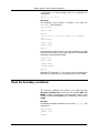
Read the initial solution
Two cases are possible :
1 - The parameters of the initial solution are introduced at the
prompt or by the commands file. Call the block
INIT(real,real,...,real) and fill, if required, the initialization
parameters table (real numbers) which follows.
2 - The initial solution is stored in a file (see Degrees of
freedom file). Define the variables MFIL, MINI, FFINI and
TASINI. Call the block INIT(real,real,...,real).
Example 1:
The initialization is done without data files and all the degrees of
freedom are set at zero ; the command is :
INIT[0]
3-4
HYDROSIM 1.0a06 - User's Guide
Chapter Chapter 3 : How to manage a simulation ?
If parameters (3 in this example) have to be specified, the
command is :
INIT[0](1.0,-2,100)
Example 2:
The stationary initial solution is stored in the ASCII file
test.deb ; the command is :
_MFIL=’test’
_MINI=’.deb’
INIT[0]
If the file is in binary format, the command
is :
_MFIL=’test’
_MINI=’.deb’
_FFINI=’BIN’
INIT[0]
In the transient context, the time has to be specified if the initial
solution stored in binary format varies with time, for example load
the solution associated with t=3h00 :
_MFIL=’test’
_MINI=’.deb’
_FFINI=’BIN’
_TASINI=10800.
INIT[0]
Remark{ XE "Remarque" } : The format of the file read by the
block INIT is identical to the format generated by the block FIN.
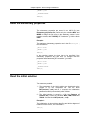
Read the boundary conditions
The boundary conditions are stored in an ASCII file (see
Boundary conditions file). Define only the variables MFIL and
MCND to assign the file name in the stationary context. In the
transient context, add TASCND { XE "transitoire" }. Call the block
COND.
Example :
the stationary boundary conditions are in the file test.prn ; the
command is :
_MFIL=’test’
_MCND=’.cnd’
COND[0]
HYDROSIM 1.0a06 - User's Guide
3-5
Chapter Chapter 3 : How to manage a simulation ?
In the transient context, the time has to be specified if the
boundary conditions vary with time, for example load the
conditions associated with t=1h00 :
_MFIL=’test’
_MCND=’.cnd’
_TASCND=3600.
COND[0]
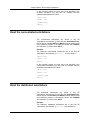
Read the concentrated solicitations
The concentrated solicitations are stored in an{ XE
"sollicitations :concentrées" } ASCII file (see Solicitations file).
Define only the variables MFIL and MSLC to assign the file name
in the stationary context. In the transient context, add TASSLC{
XE "transitoire" }. Call the block SOLC.
Example :
The stationary concentrated solicitations are in the file{ XE
"sollicitations :concentrées" } test.slc ; the command is :
_MFIL=’test’
_MSLC=’.slc’
SOLC[0]
In the transient context, the time has to be specified if the
concentrated solicitations vary with time, for example load the
solicitations associated with t=-0h30 :
_MFIL=’test’
_MSLC=’.slc’
_TASSLC=-1800.
SOLC[0]
Read the distributed solicitations
The distributed solicitations are stored in an{ XE
"sollicitations :concentrées" } ASCII file (see Solicitations file).
Define only the variables MFIL and MSLR to assign the file name
in the stationary context. In the transient context, add TASSLR{
XE "transitoire" }. Call the block SOLR.
Example :
The stationary distributed solicitations are in the file{ XE
"sollicitations :concentrées" } test.slr ; the command is :
3-6
HYDROSIM 1.0a06 - User's Guide
Chapter Chapter 3 : How to manage a simulation ?
_MFIL=’test’
_MSLR=’.slr’
SOLR[0]
In the transient context, the time has to be specified if the
distributed solicitations vary with time, for example load the
solicitations associated with t=0h00 :
_MFIL=’test’
_MSLR=’.slr’
_TASSLR=0.
SOLC[0]
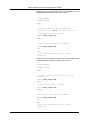
Solve the problem
The procedure to activate the solution has two steps :
1 - Mandatory step if IMPR=3. Assign a value to ILU and to
DELPRT. Activate the block PRCO.
2 - Assign a value to TINI, NPAS, IMPR, NPREC, NRDEM,
NITER,
OMEGA
and
EPSDL.
Call
the
block
SOLV(real,real,real) and fill, if wanted, the limitors table
which follows.
Example 1:
We want to run a stationary solution with a ILU matrix filled at
level{ XE "niveau :remplissage ILU" } 0, 1 preconditioning, 10
restarts, 25 iterations, a precision of 10-6 and limitors on the
variation of velocities in x and y of 0.25m/s and of 0.1m on the
water level ; the command is :
_ILU=0
_DELPRT=1.e-08
PRCO
_IMPR=3
_NPREC=1
_NRDEM=10
_NITER=25
_OMEGA=1.0
_EPSDL=1.e-06
SOLV[0](0.25,0.25,0.1)
Example 2:
We want to run a transient solution by an implicit Euler scheme{
XE "transitoire" } { XE "Euler" } (ALFA=1) to simulate a one hour
process with a one minute time step, and the simulation launch
time set at 0. We use an ILU matrix filled at level{ XE
"niveau :remplissage ILU" } 0, 1 preconditioning, 10 restarts, 25
iterations, a precision of 10-6 and limitors on the variation of
HYDROSIM 1.0a06 - User's Guide
3-7
Chapter Chapter 3 : How to manage a simulation ?
velocities in x and y of 0.25m/s and of 0.1m on the water level ;
the command is :
_ILU=0
_DELPRT=1.e-08
PRCO
_ALFA=1
_TINI=0
_DPAS=60
_NPAS=60
_IMPR=3
_NPREC=1
_NRDEM=10
_NITER=25
_OMEGA=1.0
_EPSDL=1.e-06
SOLV[0](0.25,0.25,0.1)
Remark{ XE "Remarque" } : The intermediate solutions are not
accessible in post-solution ; only the final solution can be
exploited later.
Print the results
The print operation of each type of results consists in defining the
name of the results file{ XE "fichier:résultats" } (see Structure of
file names) with the appropriate variables, and activating the
appropriate block to proceed with the printing. Here are the
various types of results that can be printed by HYDROSIM :
•
Print the degrees of freedom
•
Print the estimate of the numerical errors
•
Print the post-processing
•
Print the residuals
•
Print the function current
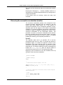
Print the degrees of freedom
The degrees of freedom are stored in a binary file (see Degrees
of freedom file). Define the variables MFIL and MFIN to assign
the file name. Call the block FCRT.
3-8
HYDROSIM 1.0a06 - User's Guide
Chapter Chapter 3 : How to manage a simulation ?
Example :
The degrees of freedom must be stored in the
test.fin ; the command is
ASCII file
_MFIL=’test’
_MFIN=’.fin’
FIN[0]
or in a binary file
_MFIL=’test’
_MFIN=’.fin’
_FFFIN=’BIN’
FIN[0]
Remark{ XE "Remarque" } : The format of the file generated by
the block FIN is identical to the format read by the block
INIT(real,real,...,real).
Print the estimate of the numerical errors
The numerical errors are stored in an ASCII file (see Numerical
errors file). Define the variables MFIL and MERR to assign the
file name. Call the block ERR.
Example :
The numerical errors must be stored in the file test.err ; the
command is :
_MFIL=’test’
_MERR=’.err’
ERR[0]
Print the post-processing
The post-processing is stored in an ASCII file (see Postprocessing file). Define the variables MFIL and MPST to assign
the file name. Call the block POST.
Example :
The results of the post-processing must be stored in the file
test.pst ; the command is :
_MFIL=’test’
_MPST=’.pst’
HYDROSIM 1.0a06 - User's Guide
3-9
Chapter Chapter 3 : How to manage a simulation ?
POST[0]
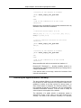
Print the residuals
The residuals are stored in an ASCII file (see Residuals file).
Define only the variables MFIL and MRES to assign the file name
in the stationary context. In the transient context, add DPAS and
ALFA{ XE "transitoire" }. Call the block RESI.
Example 1:
The residuals associated with a stationary solution must be
stored in the file test.res ; the command is :
_MFIL=’test’
_MRES=’.res’
RESI[0]
Example 2:
The residuals associated with a transient solution calculated with
an implicit EULER scheme (ALFA=1) and a one minute time
step, must be stored in the file test.res ; the command is :
_MFIL=’test’
_MRES=’.res
_ALFA=1.0
_DPAS=60.’
RESI[0]
Print the function current
The function current is stored in a read/write ASCII file (see
Function current file). Define the variables MFIL and MFCR to
assign the file name, and the solution variables ILU, NRDEM,
NITER, EPSDL and OMEGA. Call the block FCRT.
Example 1 :
The function current, after having been calculated by a direct
method, must be stored in the file test.fcr ; the command is :
_MFIL=’test’
_MFCR=’.fcr’
_ILU=-1
_NRDEM=1
_NITER=1
3-10
HYDROSIM 1.0a06 - User's Guide
Chapter Chapter 3 : How to manage a simulation ?
_OMEGA=1
_EPSDL=1.E-06
FCRT[0]
Example 2 :
The function current, after having been calculated by an iterative
method, economical in terms of memory space, must be stored in
the file test.fcr ; the command is :
_MFIL=’test’
_MFCR=’.fcr’
_ILU=0
_NRDEM=25
_NITER=100
_OMEGA=1
_EPSDL=1.E-06
FCRT[0]
! call several FCRT if the problem did not
! converge
Remark : The result file associated with FCRT is a read/write file.
If the file already exists before calling FCRT, you must make sure
that the information it contains is conform (see Function current
file). It should contain the initial solution of the function current.
HYDROSIM 1.0a06 - User's Guide
3-11
Chapter Chapter 4 : How to obtain a hydrodynamic solution?
Chapter 4 How to obtain a hydrodynamic
solution?
This chapter provides precautions that should be observed to
obtain a hydrodynamic solution in the best delays.
Past experience has shown that hydrodynamic modeling by
finite elements is not a linear process, but rather an iterative
procedure which should converge. A simulation is a complex
activity which implies the construction of a terrain numerical
model, a hydrodynamic mesh and boundary conditions. Then the
model must be given an initial run, the solution processed and
analyzed and the model validated. The following step, the most
delicate, is to calibrate the model. When all these steps have
been achieved, the model can be used as a prediction tool..
We will concentrate on certain dispositions which deserve to be
consulted to execute a hydrodynamic simulation efficiently:
•
How to validate the input data (preliminary phase)?
•
How to give the model an initial run?
•
How to converge the solution?
•
How to validate the model?
•
How to adjust the model (calibration)?
•
Frequently asked questions
How to validate the input data (preliminary
phase)?
"Input data" are the data transmitted directly to the simulator in
the command file. These are not the basic terrain data used to
build the terrain numerical model. They must be controlled
directly by the software used to prepare the input data for
HYDROSIM. In practice, you must make sure that :
1 - the finite element used for the mesh is available in the library
of elements of HYDROSIM ;
2 - the skin of the hydrodynamic mesh represents the exact
outline of the simulation domain ;
3 - the hydrodynamic mesh covers the entire flow bed ;
4 - the projection of the terrain numerical model on the
hydrodynamic mesh does not generate corrupted values ;
HYDROSIM 1.0a06 - User's Guide
4-1
Chapter Chapter 4 : How to obtain a hydrodynamic solution?
5 - you launch a simulation with HYDROSIM with the
instructions to read the data and print the post-processing ;
6 - you analyze the solution and verify if it respects the boundary
conditions and the initial conditions.
How to give the model an initial run?
The initial run must calculate the very first solution on the
simulation domain{ XE "solution" }. It is an important step
because, in certain cases, this first solution may become the
initial solution to search for other states. This is especially the
case when modeling long river reaches with a with a strong slope
(water level difference of several meters).
For a successful initial run of the model, boundary conditions and
initial conditions must be chosen with great care :
•
Scenarios of boundary conditions
•
Scenarios of initial conditions
Scenarios of boundary conditions
The boundary conditions are introduced on the outline of the
simulation domain, i. e. on the mesh skin. Physically, the domain
outline is formed by a series of open and solid boundaries. Each
type of boundary requires a special treatment :
•
Solid boundary
•
Open boundary
Solid boundary
On a solid boundary (shore), the water level is never imposed.
However, one or the other of the following conditions is
introduced :
•
qn = 0 (normal flux nil at the boundary or impermeability
condition{ XE "conditions :imperméabilité" })
•
qn = qt = 0 (the normal and tangential components of the flux
are nil or no flow conditions{ XE "conditions :adhérence" })
In practical studies of rivers, an impermeability condition is more
appropriate because it ignores the limit layer developing along
solid boundaries. A limit layer is subjected to strong gradients
and it is very thin compared to the dimensions of the study
domain. Very often, this small zone offers little interest to the
model designer.
4-2
HYDROSIM 1.0a06 - User's Guide
Chapter Chapter 4 : How to obtain a hydrodynamic solution?
However, in the case where the flow is confined to a cavity, a
groin or around a stopping point, a no flow condition is then
required.
Remember that a limit layer badly captured (use of a no flow
condition on a coarse mesh) will result in artificially slowing down
the flow and over elevating the water level. If the modeling
exercise is to reproduce the limit layer, the mesh must be refined
in the normal flow direction{ XE "couche limite" }.
Remark{ XE "Remarque" } : The condition of nil flux on a solid
boundary is implicit in HYDROSIM and does not have to be
specified explicitly.
Open boundary
On a downstream open boundary, the water level is always
imposed{ XE "niveau :aval" }. The direction of flow can be
imposed via the tangent flux, or kept free :
•
h = haval
•
qt = 0 (tangential component of nil flux) or free
In sub-critical flow regime{ XE "régime :fluvial" } (Froude
Number{ XE "Froude" } < 1), on an upstream open boundary, we
always impose either the water level or a solicitation in discharge,
and eventually, the direction of flow :
•
h = hamont , a solicitation in normal flux qn.
•
qt=0 (tangential component of nil flux)
while in rapid flow{ XE "régime :torrentiel" } (Froude{ XE "Froude"
} Number > 1), the water level and the normal flux must be
imposed :
•
h=hamont
•
qn=qn amont (normal component of the imposed flux)
The conditions on the flux were expressed in the normal-tangent
{ XE "repère" } coordinate system because it is the most
appropriate, in the sense that it reflects the most simply the flow
conditions. Only in very theoretical cases is it possible to fix
conditions on the flux in a cartesian coordinate system mixed ({
XE "repère" }to within a 90 degree rotation) with the normaltangent system{ XE "repère" }.
A solicitation applies when the degree of freedom is not imposed
explicitly, In certain cases, it can be an advantage since the
resulting system of finite element equations is less constrained
and more friendly for the solution procedure.
Remark{ XE "Remarque" } : The water level imposed has
precedence over the solicitation on discharge, if they are
imposed at the same time on a same boundary.
HYDROSIM 1.0a06 - User's Guide
4-3
Chapter Chapter 4 : How to obtain a hydrodynamic solution?
Scenarios of initial conditions
The initial conditions must be chosen with great care to ensure
the delicate{ XE "conditions :initiales" } convergence{ XE
"convergence" } of the solution process. In HYDROSIM, four (4)
strategies of initialization are proposed :
•
Static solution (static water body)
•
Quasi linear solution
•
Improved quasi-linear solution
•
Reference solution
Static solution (static water body)
In this situation, the fluid is resting ; the expression for the entire
domain is :
•
qx0=qy0=0
•
h0=constant
Example :
The HYDROSIM command file is :
! no initialization file to read
!_MINI=’’
INIT(0.0 ,0.0 , constant, 0.0, 0.0, 0.0, 0.0)
This form can be sufficient when the slope in the modelized
domain is weak (a few centimeters at most). The choice of the
value given to h is generally consistent with the water level
imposed at the open boundaries.
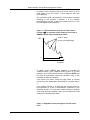
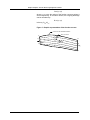
Quasi linear solution
In this situation, the water level and the slope are roughly known
a priori. At all points of the simulation domain, the water level is
given by the equation of a flat surface :
•
h(x)=h0+Sx(x-x0)+Sy(y-y0)
where h0 is the water level at the coordinate (x0,y0). Sx and Sy are
the slopes in x and y respectively.
The flux are approximated by the program using the Chézy{ XE
"Chézy" }-Manning law{ XE "Manning" } :
•
4-4
qxi=(Sxi/(Sx2+Sy2)0,25).(H5/3).(1/n), i=1,2
HYDROSIM 1.0a06 - User's Guide
Chapter Chapter 4 : How to obtain a hydrodynamic solution?
where H represents the depth and n the Manning coefficient{ XE
"Manning" }.
Example :
The command file is :
! no initialization file to read
!_MINI=’’
INIT(0.0 ,0.0 , h0, Sx, Sy, x0, y0)
This form can be very interesting in straight channel since it
accelerates the convergence process if the initial solution is near
the solution of the problem.
Warning{ XE "Mise en garde" } : in rivers, this approach is not
desirable since it does not take into account the complexity of the
stream and thalweg profile. The lack of pertinence of the
predicted initial solution may compromise the convergence
process.
Improved quasi-linear solution
It is a generalization of the approach Quasi linear solution in the
sense that the water level and the slopes are known a priori. The
approximation of flux is the same as in the quasi-linear solution.
However, the difference is that the slopes are variable in the
simulation domain. In this case, the initialization must be done
from a n initialization file. The information must contain the water
level values and the flux set at zero (see file format).
Example :
The command file is :
! initial solution stored in file ’solinitiale.deb’ in format ASCII
_FFINI=’ASCII’
_MINI=’sol-initial.deb’
INIT
This form of initialization is very interesting as it offers an
appreciable calculation time saving in the large scale modeling
projects.
Reference solution
The solution proceeds from a simulation previously conducted. It
is the case when conducting a sensitivity study (to discharge or
to regulated conditions) and wanting to switch from one state to
another.
Example :
The command file is :
! initial solution stored in file
HYDROSIM 1.0a06 - User's Guide
4-5
Chapter Chapter 4 : How to obtain a hydrodynamic solution?
! ’sol-reference.deb’ in format ASCII
_FFINI=’ASCII’
_MINI=’sol-reference.deb’
INIT
This form of initialization is practical when attempting to reach
solution convergence with several steps. It can also be useful
when moving from one event to another by slightly modifying the
hydraulic data.
How to converge the solution?
•
Solution method
•
Solution update
•
Behaviour of the solver
•
Has convergence been reached?
•
Advanced solution strategies
•
Practical advice
Solution method
In HYDROSIM, the solution method of the algebraic equation
system is done by the iterative non-linear GMRES method,
according to a "Newton-Inexact" scheme, with preconditioning.
The different aspects of the method are :
•
GMRES
•
Preconditioning matrix
•
Memory space
•
Precision
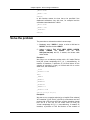
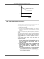
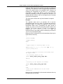
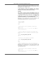
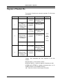
GMRES solution algorithm
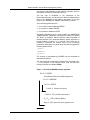
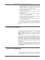
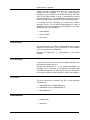
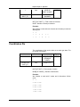
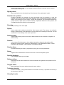
The functioning of the GMRES{ XE "GMRES :algorithme" }
solution algorithm is presented on Figure 1. There are three
loops. The first loop is driven by the variable NPREC, the second
by the variable NRDEM an the third by NITER which cannot
exceed the value of TNDF{ XE "NDLT" }, the total number of
degrees of freedom (variable). The variable NITER plays a
double role as, not only does it fix the number of iterations, but it
4-6
HYDROSIM 1.0a06 - User's Guide
Chapter Chapter 4 : How to obtain a hydrodynamic solution?
also governs the dimension of the solution sub-space equal to
the product of NITER by TNDF{ XE "NDLT" }.
The first loop is dedicated to the calculation of the
Preconditioning matrix, the second to the Solution update and the
third to the calculation of the solution sub-space of the type
Krylov by the GMRES{ XE "GMRES :paramètres" } method.
The functioning parameters are :
1 - the number of preconditioning NPREC
2 - the number of restart NRDEM
3 - the number of iterations NITER
The theory stipulates that for a linear problem, the GMRES{ XE
"GMRES :théorie" } algorithm converges at a maximum of TNDF{
XE "NDLT" } iterations, which would be totally impossible in
practice because of the exorbitant Memory space required for a
normal problem. However, in a non-liner case, there are no
methods to determine the optimal values of the functioning
parameters. Experience on a wide range of problems suggest the
following default values :
_NPREC=1
_NRDEM=25
_NITER=25
The number of preconditioning (NPREC) can be increased for
important simulations.
The stop criteria of the algorithm is based on the increment norm,
i. e. the progress of the solution which must be below the
Precision fixed by the variable EPSDL.
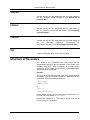
Figure 1 : Non-linear GMRES solution algorithm.
Do I1=1,NPREC
Calculation of the preconditioning matrix
Do I2=1,NRDEM
Do I3=1,NITER
Calcul. of solution sub-space
Calcul.of ∆ U (solution increment)
Ui2=Ui2-1+∆U (solution update)
Stop if || ∆U||<precision (convergence test)
HYDROSIM 1.0a06 - User's Guide
4-7
Chapter Chapter 4 : How to obtain a hydrodynamic solution?
Preconditioning matrix
The preconditioning matrix plays a very important role in the
GMRES solution algorithm{ XE "GMRES :préconditionnement" }.
A good preconditioning greatly improves the performances of the
solver. For example, two given preconditioning matrix can make
the problem either converge or diverge. There is divergence of
the solution algorithm if the increment norm tends to increase
(explosion).
In the case of the Saint-Venant equations{ XE "Saint-Venant" },
the experience shows that the ILU preconditioning matrix, with
minimum fill level (ILU=0), is efficient. The command file :
_ELTYP=’SVCRNM’
:
_ILU=0
PRCO
_IMPR=3
:
If the Memory space allows it, better results are obtained with the
maximum fill level (ILU=-1). In this case, to minimize calculation
and memory requirements (related to the matrix band width), the
commands are :
ELTYP=’SVC’
:
_ILU=-1
PRCO
_IMPR=3
:
In the case when even a ILU matrix with the minimum fill level{
XE "niveau :remplissage ILU" } (ILU=0) cannot be exploited
because of memory capacity problems, the compromise to make
is to use a diagonal preconditioning (see IMPR).
Remark{ XE "Remarque" } : The performance of the ILU
preconditioning is strongly influenced by the numbering of the
mesh nodes. To obtain better results, it is recommended to use a
numbering algorithm minimizing the band width.
Memory space
In the solution algorithm, the ILU preconditioning matrix and the
dimension of the solution sub-space via NITER determine the
memory space required for the solution procedure..
The memory space needed to store the ILU matrix with a n fill
level (ILU=n) is about :
4-8
HYDROSIM 1.0a06 - User's Guide
Chapter Chapter 4 : How to obtain a hydrodynamic solution?
σ.((3/2).NKGP{ XE "NKGP" }+(3.n+1).NDLT{ XE "NDLT" }+1/2)
in Megabytes{ XE "mégabytes" } ;
while that associated with the solution sub-space is given by :
σ.NITER.NDLT{ XE "NDLT" }
20
where σ=8/2 is the conversion coefficient from real words to
Megabytes and NKGP{ XE "NKGP" } the number of non-null
terms in the ILU matrix. This information can be found in the
output file associated with the command :
_ILU=0
PRCO[0]
Precision
The precision applicable to the iterative process of the Solution
update is defined using the variable EPSDL. The greater the
precision, the greater the volume of calculation.
For the simulation of theoretical problems, EPSDL is given a
value in the order of :
_EPSDL=1.E-10
For the efficient simulation of real cases, the value temporarily
given is the order of :
_EPSDL=1.E-03
and, nearing the solution, the value of{ XE "solution" } EPSDL is
progressively reduced to the desired precision Which may
typically be in the vicinity of :
_EPSDL=1.E-06
Solution update
In the solution algorithm (see Figure 1), the solution updte is
done after each restart, as follows ::
Ui2=Ui2-1+∆U
where Ui2 designates the vector solution at the (i2) th restart and
∆U the solution increment.
However, HYDROSIM proposes to modulate the solution update,
which may be very useful when the solution varies greatly and/or
the non-linearities are important. The calculation of the solution
increment ∆U is as follows :
∆U= signe(∆U) max(∆Umax,|ω∆U|)
where ∆Umax is the limitor. A limitor is associated with each type
of variable (degree of freedom).
HYDROSIM 1.0a06 - User's Guide
4-9
Chapter Chapter 4 : How to obtain a hydrodynamic solution?
Therefore, two possibilities are offered to intervene during the
solution update :
•
Relax the solution update
•
Limit
Relax the solution update
To relax the solution means "to tone down" the amplitude of the
increment ∆U. The procedure of the solution update is as
follows :
Ui2=Ui2-1+ω∆U
where ω is the relaxation factor.
Example :
We want to sub-relax the solution with a factor of 0.8 :
_OMEGA=0.8
In practice, the sub-relaxation (ω<1) allows the solver to better
converge when the problem is difficult. On the other hand, it
slows down the solution process, especially when nearing the
solution..
Limit the solution update
The technique consists in imposing an absolute limit to the value
of the increment ∆U.
Example :
We want to limit the solution update ∆U with values of ∆U max of
0.25 and 0.1 on the flux (qx,qy) and the water level (h)
respectively :
SOLV[0](0.25, 0.25, 0.1)
In practice, the limitor intervenes in the solution update process
only when the increment ∆U exceeds the limitor ∆Umax. Also,
nearing the solution, the solution process is not slowed down.
The limitation of the solution update can be done along with the
relaxation.
Behaviour of the solver
Figure 2 presents the typical convergence curve of{ XE
"convergence" } GMRES{ XE "GMRES :comportement" }
associated with a preconditioning of the type ILU.
4-10
HYDROSIM 1.0a06 - User's Guide
Chapter Chapter 4 : How to obtain a hydrodynamic solution?
In general, there is a peak of the norm of{ XE "norme" } ∆U at
each update of the ILU matrix, in other words at each new
preconditioning.
The convergence{ XE "convergence" } of the problem is reached
according to the precision ε retained, if at the following
preconditioning, the peak of the norm remains inferior to ε (see
Has convergence been reached?).
Figure 2 : Typical behaviour of the norm of the solution
increment ∆U as a function of the iterations in the case of
GMRES with the ILU preconditioning matrix.
||∆U||
Peak of norm
at new preconditioning
ε
iterations
In certain cases, GMRES may stagnate or oscillate{ XE
"GMRES :stagne" } { XE "GMRES :oscille" }(Figure 3). The first
possible cure is to increase the number of iterations NITER. Not
only does this parameter extend the calculation loop, it also
increases the solution sub-space.
If the result is the same, modify the upper bound of viscosity
upward first, then downward if necessary{ XE "viscosité :borne"
}.
If the problem persists, it is likely that the solution cannot be
found because of a lack of discretization somewhere in the
simulation domain. You must then visually identify the problem
zone (zone with high residuals). Next, you must refine the mesh
locally and re-launch the simulation.
Figure 3 : Stagnation of the convergence process of the
norm.
HYDROSIM 1.0a06 - User's Guide
4-11
Chapter Chapter 4 : How to obtain a hydrodynamic solution?
||∆U||
stagnation of the norm
ε
iterations
Has convergence been reached?
To confirm that the convergence of the calculated solution has
been reached numerically, you must make sure that :
1 - GMRES has converged ;
2 - The norm of the residuals associated with each degree of
freedom{ XE "norme" } (qx, qy et h) is at most in the same
order as ε.
If there is convergence, the{ XE "convergence" } simulation is
ended.
In the case of local convergence only, the simulation must be relaunched starting from the last solution, and the number of
iterations NITER must be increased. Repeat this procedure if
needed.
If the problem persists, visually analyze the results ; two
scenarios are possible :
1 - The results are generally valid. In this case, isolate the zones
with high residuals. Refine the mesh in these zones, relaunch the simulation on this new mesh. Repeat this
procedure, if needed.
2 - Locally, the results are bad (velocity vectors shooting in all
directions, parasitic oscillations of the water level). In this
case, you must re-launch the simulation with a new
initialization :
a) by increasing the upper bound of viscosity if the problem
zone is located in the flow bed{ XE "viscosité :borne" }.
b) by decreasing the upper bound of viscosity if the problem
zone is located near the shore.
4-12
HYDROSIM 1.0a06 - User's Guide
Chapter Chapter 4 : How to obtain a hydrodynamic solution?
Advanced solution strategies
In certain cases, the solution of the problem is not automatic.
You must then adopt a solution strategy using intermediate
solutions. The choice of the strategy is on a case by case basis.
Four solution strategies have been identified.
•
Driven by the downstream water level
•
Driven by the convective acceleration (inertia)
•
Driven by the upper bound of viscosity
•
Driven by the time step
Driven by the downstream water level
This strategy is generally used in the phase of the initial run of
the model, during modeling of small streams or long river
reaches (several km), where the water level difference between
the upstream and downstream boundaries is in meters as shown
on Figure 4.
Figure 4 : : Successive water lines on a profile.
Upstrem level
Initial water line
Intermediate water lines
Final water line
bed
Downs. lev.
The boundary condition on the downstream water level is the
parameter to modify.
Example :
The upstream water level is at the elevation{ XE "niveau :amont"
} 155 m and the downstream level targeted at the elevation 150
m. We begin with a downstream level of 155 m. To calculate the
solution in permanent regime, we intend to modify the
downstream level by increment of -0.50 m. The command file
reads :
HYDROSIM 1.0a06 - User's Guide
4-13
Chapter Chapter 4 : How to obtain a hydrodynamic solution?
Beginning of the command file for the first simulation driven by
the downstream water level { XE "niveau :aval" }
:
_ELTYP=’SVCRNM’
_STEMP=’STATIQ’
FORM
:
! Initial condition :Initial model run
INIT[0](0.0, 0.0, 155.0, 0.0, 0.0, 0.0, 0.0)
! Downstream condition h=154.5m
_MCND=’haval_154p5.cnd’
COND[0]
:
! Printing of the degrees of freedom
_MFIN=’haval_154p5.deb’
FIN
STOP
! End of the command file of the first
simulation
Beginning of the command file for the second simulation driven
by the downstream water level { XE "niveau :aval" }
:
_ELTYP=’SVCRNM’
_STEMP=’STATIQ’
FORM
:
! Initial condition :Solution of the first
simulation
_MINI=’haval_154p5.deb’
INIT[0]
! Downstream condition h=154,0m
_MCND=’haval_154p0.cnd’
COND[0]
:
! Printing of the degrees of freedom
_MFIN=’haval_154p0.deb’
FIN
STOP
! End of the command file of the first
simulation
4-14
HYDROSIM 1.0a06 - User's Guide
Chapter Chapter 4 : How to obtain a hydrodynamic solution?
We repeat until the downstream water level reaches the elevation
150 m.
Remark{ XE "Remarque" } : Another possibility would be to
automate all the operations described above by inserting them in
a single command file.
If the solution does not converge, reduce the water level
increment.
Driven by the convective acceleration (inertia)
The convective acceleration (inertia) is the component of the
movement equation associated with the changes in the flow
section (sills, pools, bridge section, etc...). The influence of
convective acceleration on the convergence problems is major,
especially when the flow regime is near critical or supra-critical
conditions. To by-pass the difficulty, the solution is calculated in
successive steps by gradually increasing the effects of the
convective acceleration on the intermediate solution. This
procedure is known as convective acceleration driven solution,
where the activation factor of the convection varies in the range
[0,1]. Inertia is inactive when the factor is equal to 0 (Stokes
problem{ XE "Stokes" }) and completely activated at 1.
Example :
The upstream water level is at elevation 155 m and the
downstream water level is at 150m. To calculate the solution in
permanent regime, we choose the approach « Driven by the
downstream water level » and the level of activation of the
convection in the phase of downstream water level reduction
remained at 0. The solution obtained is stored in the degrees of
freedom file haval_150p0.deb. Next, we add the effects of
convection by increments of 0.25. The command file reads :
Beginning of the command file of the first simulation driven by
activation of the convective acceleration
:
_ELTYP=’SVCRNM’
_STEMP=’STATIQ’
FORM
:
! Convection factor equal to 0.25
PRGL[0](9.8, 0., 0., 1., 0.,1.e-6 ,100, 10.,1.,
0.25,0.5,1e-05,1e-3)
:
! Initial condition :Solution with haval=150,0m
and convection
! null.
_MINI=’haval_150p0.deb’
INIT[0]
HYDROSIM 1.0a06 - User's Guide
4-15
Chapter Chapter 4 : How to obtain a hydrodynamic solution?
:
! Printing of the degrees of freedom
_MFIN=’haval_150p0_conv_0p25.deb’
FIN
STOP
! End of the command file of the first
simulation
Beginning of the command file of the second simulation driven by
activation of the convective acceleration
:
! Convection factor equal to 0.50
PRGL[0](9.8, 0., 0., 1., 0.,1.e-6 ,100, 10.,1.,
0.50,0.5,1e-05,1e-3)
:
! Initial condition :Solution of the first
simulation
_MINI=’haval_150p0_conv_0p25.deb’
INIT[0]
:
! Printing of the degrees of freedom
_MFIN=’haval_150p0_conv_0p50.deb’
FIN
STOP
! End of the command file of the second
simulation
We proceed like this until the convection level reaches 1.0.
Remark{ XE "Remarque" } : Another possibility would be to
automate all the operations described above by inserting them in
a single command file.
If the solution does not converge, reduce the increment of the
convective acceleration.
Driven by the upper bound of viscosity
The term turbulent diffusion in the equations takes into account
the constraints of shear stress and of compression related to the
gradients of velocity in the flow (vicinity of a strong current, or
zone of lentic water, for example). The turbulent viscosity is the
key parameter of this term of equilibrium, and it is automatically
calculated HYDROSIM. However, it can be useful to modify its
value to improve convergence of the solution.
The calculation of a stable solution in permanent regime is
achieved by giving a high value to the upper bound of the
viscosity. The effect of an excessive viscosity is to artificially
4-16
HYDROSIM 1.0a06 - User's Guide
Chapter Chapter 4 : How to obtain a hydrodynamic solution?
inflate the water level and to smoothen the flow by masking its
complexity. The objective is then to progressively decrease the
value of the upper bound to an acceptable value. However, by
releasing the complexities of the flow (e. g. re-circulation),
convergence is made more difficult. In fact, mesh size may
hinder the possibility of solving a complex flow structure. It is
admitted that the minimum value of the upper bound of viscosity
is the limit of convergence.
The value given to launch the very first simulation is empirical.
Example :
The upstream water level is at elevation 155 m and the
downstream water level is at 150m. To calculate the solution in
permanent regime, we choose the approach « Driven by the
downstream water level », maintaining the upper bound of
viscosity at a value of 100 m2/s during the phase of water level
reduction. The solution obtained is stored in the degrees of
freedom file haval_150p0_nusup_100p0.deb. Next, we
reduce the value of the upper bound of viscosity by increment of
10 m2/s. The command file reads :
Beginning of the command file of the first simulation driven by the
upper bound of viscosity
:
_ELTYP=’SVCRNM’
_STEMP=’STATIQ’
FORM
:
! Upper bound of viscosity equal to 90
PRGL[0](9.8, 0., 0., 1., 0.,1.e-6 ,90, 10.,1.,
1.0,0.5,1e-05,1e-3)
:
! Initial condition :Solution calculated with
the upper bound
! of viscosity equal to 100
_MINI=’haval_150p0_nusup_100p0.deb’
INIT[0]
:
! Printing of the degrees of freedom
_MFIN=’haval_150p0_nusup_90p0.deb’
FIN
STOP
! End of the command file of the first
simulation
Beginning of the command file of the second simulation driven by
the upper bound of viscosity
:
HYDROSIM 1.0a06 - User's Guide
4-17
Chapter Chapter 4 : How to obtain a hydrodynamic solution?
! Upper bound of viscosity equal to 80
PRGL[0](9.8, 0., 0., 1., 0.,1.e-6 ,80,
10.,1.,1.0,0.5,1e-05,1e-3)
:
! Initial condition :Solution of the first
simulation
_MINI=’haval_150p0_nusup_90p0.deb’
INIT[0]
:
! Printing of the degrees of freedom
_MFIN=’haval_150p0_nusup_80p0.deb’
FIN
STOP
! end of the command file of the second
simulation
We proceed like this until convergence becomes difficult, or that
the degree of adequation with the available measurements
(validation{ XE "validation" }) is satisfactory.
Remark{ XE "Remarque" } : Another possibility would be to
automate all the operations described above by inserting them in
a single command file.
If the solution does not converge, reduce the increment of the
upper bound of viscosity.
A possible consequence of the reduction of the upper bound of
viscosity is the degradation of mass conservation.
Driven by the time step
A permanent flow can be solved in time if the transient phase has
no interest. The stationary solution is sought for with this method.
Example :
The upstream water level is at elevation 155 m and the
downstream water level is at 155 m. We start from a hydrostatic
initial condition with a water body at elevation 155 m. To
calculate the solution in permanent regime, we vary the
downstream water level at the rate of 0.50 m per hour. It would
take 10 hours for the downstream water level to reach 150 m
and about 5 more hours for the flow to reach a permanent
regime. With a time step of 900 s, a minimum of 660 simulation
time step is needed. The command file reads :
Beginning of the command file of the simulation driven by the
time step { XE "pas de temps" }
:
_ELTYP=’SVCRNM’
_STEMP=’EULER’
4-18
HYDROSIM 1.0a06 - User's Guide
Chapter Chapter 4 : How to obtain a hydrodynamic solution?
FORM
:
! Initial condition :Model initial run
INIT[0](0.0, 0.0, 155.0, 0.0, 0.0, 0.0, 0.0)
! Downstream condition h=155.0m à t=0h00 et
150.0m à t=10h00.
! Downstream water level at beginning 155.0m
_TASCND=0
_MCND=’hav_155p0_t00h00-150p0_t10h00.cnd’
COND[0]
:
! parameters of solution in time
_TINI=0
_DPAS=900
_NPAS=100
:
STOP
! End of command file
Remark{ XE "Remarque" } : If the solution does not converge,
reduce the time step{ XE "pas de temps" }. If the problem
persists, reduce the rate of downstream water level reduction.
Practical advice
This advice concerns long duration simulations, for example a
night long job. To avoid any unexpected problem which might
induce the loss of several hours of calculation, it is strongly
recommended to print periodically the degrees of freedom, in
different files if disk space is available. After a power failure, it will
be possible to re-launch the simulation from the most recent
solution obtained or acceptable.
Example :
For a same volume of calculation, instead of command 1 :
!---- command 1 : single printing of dof in
test.fin
_NPREC=3
SOLV[0](0.25,0.25,0.1)
_MFIL=’test’
_MFIN=’.fin’
FIN[0]
HYDROSIM 1.0a06 - User's Guide
4-19
Chapter Chapter 4 : How to obtain a hydrodynamic solution?
use :
!---- command 2 : periodical printing of dof in
test.fin#i.
_MFIL=’test’
_NPREC=1
SOLV[0](0.25,0.25,0.1)
_MFIN=’.fin#1’
FIN[0]
SOLV[0](0.25,0.25,0.1)
_MFIN=’.fin#2’
FIN[0]
SOLV[0](0.25,0.25,0.1)
_MFIN=’.fin#3’
FIN[0]
How to validate the model?
A converged solution is not necessarily valid ; in other words, the
solution calculated may lack objectivity. The validation procedure
intends to verify the degree of similarity between the terrain
observations and the simulation results under the same
hydrodynamic conditions.
For example, in a lake where the slope is very gentle (in the
order of 10-6 to 10-5 m/m), a difference of 10 cm between the
simulated levels and the values observed may not be acceptable.
However, it would be a reasonable difference in a mountain
stream with a much steeper slope (in the order of 10-3 to 10-2
m/m).
If the solution of initialization calculated is judged acceptable as
first approximation, then we can move to the calibration step
which, by various adjustments brought either to the terrain model
or to the values of the model parameters, will refine the solution
and bring it closer to actual measurements.
If, for any reason, the solution of initialization does not seem
acceptable (unrealistic flow facies, excessively high or low water
level, parasitic oscillations or extreme values of the
hydrodynamic variables, for example), you must continue the
exercise of initialization until satisfactory.
In addition to incoherent flow directions (arrows burst in all
directions without any logic), you must make sure that :
1 - the terrain topography is properly represented on the
hydrodynamic mesh ;
4-20
HYDROSIM 1.0a06 - User's Guide
Chapter Chapter 4 : How to obtain a hydrodynamic solution?
2 - in the case of very wide rivers, the Coriolis force, which
applies perpendicular to movement to the right in the
northern hemisphere and the opposite in the southern
hemisphere, is taken into account{ XE "Coriolis" } ;
3 - the wind strength , which accelerates, slows down or diverts
the flow, is taken into account ;
4 - the presence of aquatic plants, which slow down the flow, is
taken into account ;
5 - the surface ice cover, which reduces the depth and increases
the flow velocity, is taken into account ;
6 - the transit discharge at boundary conditions level-level has
the proper value (see Control of mass ) ;
7 - the natural boundaries of the flow delineated by the isoline
H=0 are correctly positioned ;
8 - flow is absent in « drying » zones (Control of Drying/Wetting).
If, after the necessary corrections, the systematic and
unacceptable bias persists, then you should question the terrain
data.
Control of mass balance
The mass balance gives a good idea of the quality, in terms of
physics, of a solution. In the output file result.out in the block
POST, HYDROSIM returns the error on the discharge over the
entire simulation domain and gives the entering and outgoing
discharges.
There could be a very good level of convergence, and yet a
mediocre quality solution. To correct the problem, first identify the
problem zones. This is done by viewing the local and global
mass balance. Second, analyze the spatial distribution of the
errors of mass conservation. Next, refine the zones judged
deficient. Then, use the same solution strategy as on the
preceding mesh.
The block of error estimates indicates if the solution may change
by refining the mesh. The units of errors are identical to those of
the variables to which they are associated : m2/s for flux and m
for the water level.
Control of Drying/Wetting
The Drying/Wetting model is governed by the penalization
(strong increase) of the Manning coefficient in the dry zones.
HYDROSIM 1.0a06 - User's Guide
4-21
Chapter Chapter 4 : How to obtain a hydrodynamic solution?
Although non-significant, there always persists a form of flow in
the dry zones. The penalization must be sufficiently high to reach
this objective in the « drying » zones.
If after examining a solution, the discharge in the « drying »
zones is found to be too high, the penalization value must be
increased until the quality criteria desired is reached.
Example :
We consider a solution involving Drying/Wetting zones. The
analysis of the solution obtained with a penalization coefficient of
10 reveals a significant flow in the dry zone. The solution stored
in the file sol_ref_penman_10p0.deb is improved by
increasing the penalization value of the Manning{ XE "Manning" }
coefficient by increment of 5. The command file reads :
Beginning of the command file of the first simulation with
Drying/Wetting adjustment{ XE "couvrant-découvrant" }
:
_ELTYP=’SVCRNM’
_STEMP=’STATIQ’
FORM
:
! Penalization value of Manning coefficient
equal to 15
PRGL[0](9.8, 0., 0., 1., 0.,1.e-6 ,100, 15.,1.,
1.0,0.5,1e-05,1e-3)
:
! Initial condition :Solution calculated with
penalization value of Manning coefficient equal
to 10
_MINI=’sol_ref_penman_10p0.deb’
INIT[0]
:
! Printing of the degrees of freedom
_MFIN=’sol_ref_penman_15p0.deb’
FIN
STOP
! End of command file of the first simulation
Beginning of the command file of the second simulation with
Drying/Wetting adjustment{ XE "couvrant-découvrant" } { XE
"couvrant-découvrant" }
:
! Penalization value of Manning coefficient
equal to 20.
PRGL[0](9.8, 0., 0., 1., 0.,1.e-6 ,100, 20.,1.,
1.0,0.5,1e-05,1e-3)
4-22
HYDROSIM 1.0a06 - User's Guide
Chapter Chapter 4 : How to obtain a hydrodynamic solution?
:
! Initial condition :Solution of the first
simulation
_MINI=’sol_ref_penman_15p0.deb’
INIT[0]
:
! Printing of the degrees of freedom
_MFIN=’sol_ref_penman_20p0.deb’
FIN
STOP
! End of command file of the second simulation
We proceed like this until the flow reduction in dry zones is
satisfactory.
Remark{ XE "Remarque" } : Another possibility would be to
automate all the operations described above by inserting them in
a single command file.
If the solution does not converge, reduce the increment of the
penalization of the Manning coefficient{ XE "Manning" }.
How to adjust the model (calibration)?
This step finely adjusts the physical and numerical parameters to
bring the numerical solution in concordance with the terrain data
under the same hydrodynamic conditions. There are two steps to
this operation ; adjustment of the target parameters, and control
of the solution obtained versus the terrain measurements.
Depending on the objectives of the modeling, emphasis can be
put on a specific variable of the problem : water level for flood
studies ; water level and velocities for habitat studies or
contaminant transport studies.
There are three calibration{ XE "calibration" } procedures :
•
Calibrate by the discharge
•
Calibrate by the water level
•
Calibrate by velocities
Calibrate by the discharge
In the case where the boundary conditions used are of the type
level-level, we expect that the results of the model will
correspond relatively well a priori to the measured water level.
However there remains to make sure that the solution calculated
HYDROSIM 1.0a06 - User's Guide
4-23
Chapter Chapter 4 : How to obtain a hydrodynamic solution?
transits a discharge (see How to estimate the discharge
transiting in the domain?) identical to the discharge measured in
the field.
If we have good reasons to believe that the friction coefficients
are acceptable in the state considered, and that the discharge
observed and calculated are not sufficiently close (at the
minimum the precision of the measure), the viscosity must be
adjusted by moving the upper bound upward if the calculated
discharge is overestimated, or downward if the discharge is
underestimated.
Calibrate by the water level
To calibrate the water level, you must first have calibrated by the
discharge (see Calibrate by the discharge) ;
Varying the water level is made by adjusting, in an acceptable
range, the Manning coefficient{ XE "Manning" }.
The water level will tend to rise if the Manning coefficient is
increased, and conversely if it is decreased.
The variation of the water level will be more sensitive at greater
flow velocities.
Calibrate by velocities
To calibrate by the velocities, you must have calibrated by the
discharge and by the water level (see Calibrate by the
discharge and Calibrate by the water level).
If there is a difference between the velocities measured vs
calculated, the Manning coefficient must be adjusted{ XE
"Manning" }. When it is increased, the coefficient slows down the
flow, reduces the flow velocity. Conversely, when decreased, the
flow velocity increases.
Remark{ XE "Remarque" }: The discharge and the water level
may be influenced by this operation. Modifications to the friction
coefficient must be done in a way that globally maintain the
behaviour of the model toward these two variables. An increase
of the friction coefficient in a region of the flow should be
accompanied by an equivalent decrease elsewhere{ XE
"frottement" }.
Adjust the Manning coefficient upward or downward if the
velocities are overestimated or underestimated respectively.
If the problem persists, make sure that :
4-24
HYDROSIM 1.0a06 - User's Guide
Chapter Chapter 4 : How to obtain a hydrodynamic solution?
1 - the hydrodynamic mesh is sufficiently fine to properly capture
the terrain topography and its flow resistance properties ;
2 - at the point of control, the bottom elevation projected on the
hydrodynamic mesh is identical to that measured in the field ;
3 - the mean velocity measured in the field is representative of
the mean flow in the horizontal plane, and not the result of a
singularity ;
4 - the mean velocity measured in the field was obtained from at
least three points in the water column for bottoms non
uniform grain size (the velocity measured at 0.4H above the
bottom is not always equal to the mean velocity).
Frequently asked questions
•
How to evaluate the turbulent viscosity?
•
How to minimize the level of error?
•
Has the solution diverge?
•
What is numerical viscosity?
•
What is the role of the upper bound of the viscosity?
•
What are the effects of an excessive dissipation?
•
How to estimate the discharge transiting in the domain?
How to evaluate the turbulent viscosity?
Evaluating the turbulent viscosity is always a delicate exercise
since the theory on turbulence is still a very active and open field
of research.
The software HYDROSIM proposes two classical approaches to
quantify the effect of turbulence :
1 - the constant viscosity model ;
2 - the mixing length model{ XE "longueur de mélange" }.
The model of the type mixing length seems to be closer to reality
than the model of constant turbulent viscosity since it takes into
account the local variability of the flow ; however the difficulty is
transferred to the evaluation of the mixing length.
In practice, adjusting the turbulent viscosity is part of the model
calibration process. When the problem centers on the use of the
water level, the mixing length is not required{ XE "longueur de
mélange" }. However, if you wish to improve the representation of
the velocities, this solution is recommended.
HYDROSIM 1.0a06 - User's Guide
4-25
Chapter Chapter 4 : How to obtain a hydrodynamic solution?
How to minimize the level of error?
Supposing that the model is well parameterized, the errors
affecting the solution are directly related to the variability of the
terrain data and of the geometry of the domain modelized. The
mesh refinement procedure is intended to minimize the level of
error to an acceptable proportion, as long as there are sufficient
terrain data to support it.
To avoid useless mesh refinement, which would induce
prohibitive calculation times, it is recommended to intervene
locally, where the level of error is judged too important. The
problem zones can be identified by the analysis of the distribution
of residuals, of errors of numerical approximations and of mass
balances.
Has the solution diverge?
The solution process has diverged if one or all of the following
phenomena are observed :
1 - The norm of the increment of the solution tends to increase
and even to explode ;{ XE "norme" }
2 - the norm of the residuals explode ;
3 - the mass balance is not realistic ;
4 - over the entire domain, or locally, velocity vectors shoot in all
directions ;
5 - over the entire domain, or locally, there are strong parasitic
oscillations of the water level
What is numerical viscosity?
Numerical viscosity is an adjustment coefficient of pure numerical
origin which as the dimension of a viscosity. Its role is to
condition the system of equations finite elements to make sure
that a solution exists when flow is dominated by convection{ XE
"convection" }.
The value given to numerical viscosity depends on the mesh and
the flow conditions. In HYDROSIM, numerical viscosity is
managed by the Peclet{ XE "Peclet" } number set at 0.5. The
variation of the numerical viscosity is inversely proportional to
that of the Peclet number.
4-26
HYDROSIM 1.0a06 - User's Guide
Chapter Chapter 4 : How to obtain a hydrodynamic solution?
What is the role of the upper bound of the viscosity?
The upper bound of the viscosity controls the numerical and
turbulent viscosity calculated during the solution process. An
overestimation of the viscosity values could compromise the
processus of convergence. On the opposite, an upper bound too
low could also underestimate the level of dissipation and have
the problem diverge quickly.
In practice, it is always difficult to set at the beginning of the very
first simulation the value to give to the upper bound of viscosity.
Only through a trial and error procedure can it be set properly.
What are the effects of an excessive dissipation?
The phenomenon of excessive dissipation is caused by an
overestimation of the viscosity. An excessive dissipation will
artificially inflate the water level and smoothen the flow. To
improve the results, you can modify the upper bound of viscosity
by decreasing it to the limit of convergence. This will result in
reducing the water level and developing the complex structures
of the flow as observed in real life.
How to estimate the discharge transiting in the domain?
The discharge transiting in the simulation domain is estimated by
analyzing the results of the function current. For example, Figure
5 presents a tracing of isolines, known as lines of current, of the
function current. Along a line of current, the normal flow is nil.
Thus, it may be considered that a solid boundary represents a
line of current because of the impermeability condition imposed.
A constant portion ∆Q of the total discharge transiting in the
domain flows between two lines of current of values ψi+1 and ψi+2.
The portion is determined by :
∆Q=|ψi+2-ψi+1|
Example
We consider, on Figure 5, a simulation domain where the contour
is made of two solid boundaries and two open boundaries. The
two solid boundaries are delineated by the curves AD and BC.
The open boundaries are delineated by the curve AB in entrance
and by the curve CD in exit. The discharge Q simulated in
permanent regime, which transits in the domain is a priori
unknown. To find it, simply calculate :
HYDROSIM 1.0a06 - User's Guide
4-27
Chapter Chapter 4 : How to obtain a hydrodynamic solution?
QAB=|ψA-ψB|
where ψA et ψB are the values of the function current at points A
and B respectively. In the same manner, the outgoing discharge
can be calculated by :
QCD=|ψC-ψD|
In theory, QAB=QCD.
Figure 5 : Graphic representation of the function current.
contour of the simulation domain
A
lines of current
ψi
ψi+1
Q
ψi+2
B
ψi+n
D
∆Q
Q
C
4-28
HYDROSIM 1.0a06 - User's Guide
Chapter Chapter 5 : Appendix
Chapter 5 Appendix
•
Language dictionary
•
Library of finite elements
•
Library of temporal schemes
•
Processing of transient data
•
Block dependencies
•
Example of command file
•
Formats of input files
•
Formats of results files
Language dictionary
The language dictionary of HYDROSIM proposes three work
languages :
•
HYDROSIM in English
•
HYDROSIM in Spanish
•
HYDROSIM in French
HYDROSIM in English
To use the English version (ENGlish), define the variable
LANGUE at :
_LANGUE=’.eng’
HYDROSIM in Spanish
To use the Spanish version (ESPagnol) define the variable
LANGUE at :
_LANGUE=’.esp’
HYDROSIM 1.0a06 - User's Guide
5-1
Chapter Chapter 5 : Appendix
HYDROSIM in French
To use the French version (FRanÇais), define the variable
LANGUE at :
_LANGUE=’.frc’
Library of finite elements
The library of finite elements of { XE "éléments finis" }
HYDROSIM proposes two types of finite elements{ XE "éléments
finis" } :
•
Finite element SVC
•
Finite element SVCRNM
Finite element SVC
Named SVC by reference to the Saint-Venant{ XE "SaintVenant" } equations in Conservative form.
•
How to reach it?
•
Function
•
Properties
•
Boundary conditions
•
Solicitations
•
Initial solution
How to reach it?
To reach it, in the command file, the variable ELTYP must be
defined as follows :
_ELTYP=’SVC’
Function
SVC is a six node triangular finite element distributed according
to the scheme one on each vertex and one in the middle of each
edge. It is used to discretize the two-dimensional Saint-Venant{
XE "Saint-Venant" } equations in the conservative form. It is
dedicated to the study of hydrodynamics in rivers and estuaries.
It supports the concept of Drying/Wetting of shores. It admits
5-2
HYDROSIM 1.0a06 - User's Guide
Chapter Chapter 5 : Appendix
three degrees of freedom per node, the scalar - water level, and
the vector - specific discharge.
Properties
•
Geometric
•
Global
•
Elementary
•
Nodal
Geometric
Number of dimensions NDIM{ XE "NDIM" }=2 ;
Number of nodes per element NNEL=6.
Global
Number of global properties to NPRGL=13 :
1 - gravity (9.75258282 m/s2<=g<=9.6605398m/s2)
2 - latitude
3 - constant turbulent viscosity
4 - mixing length coefficient{ XE "longueur de mélange" }
5 - mesh-related mixing length coefficient
6 - lower bound of viscosity
7 - upper bound of viscosity
8 - penalization of Manning{ XE "Manning" } coefficient for
Drying (=10)
9 - porosity for Drying(=1)
10 - convection coefficient { XE "convection" } (=1)
11 - Peclet number { XE "Peclet" } (=0.5)
12 - free surface smoothing coefficient (=10-05)
13 - minimum depth admissible (=10-03m)
Elementary
No elementary properties to read NPREL{ XE "NPREL" }=0.
Nodal
Number of nodal properties to read NPRNL{ XE "NPRNL" }=3 :
1 - terrain topography { XE "topographie du terrain" }
HYDROSIM 1.0a06 - User's Guide
5-3
Chapter Chapter 5 : Appendix
2 - Manning coefficient { XE "Manning" }
3 - ice thickness{ XE "glace" }
Boundary conditions
The boundary conditions (B. C.) are applied on the degrees of
freedom at the contour of the domain. The number of degrees of
freedom per node is NDLN{ XE "NDLN" }=3 : in the order, the
following specific discharge in x (qx), the following specific
discharge in y (qy) and the level of the free surface (h). The water
level at the nodes middle of edge is systematically imposed
internally (implicit B.C.). It is evaluated after the solution by giving
it the mean value at the node vertex to the corresponding edge.
In a situation of flow simulation in a domain with complex
geometry, the B.C. on the specific discharge q(qx,qy) must be
expressed in the normal-tangent coordinate system. In this case,
q admits qn and qt as components.
•
Solid boundary
•
Open boundary
•
Convention
Solid boundary
On a solid boundary, a condition of impermeability qn=0 is always
imposed. We can leave qt free or exploit a no flow condition
qt=qn=0 in the case of a confined flow.
Remark{ XE "Remarque" } : impermeability is the default
condition.
Open boundary
On an open boundary, the water level is always imposed. If the
flow direction is known, set qt=0
Remark{ XE "Remarque" } : on an entrance boundary, the
discharge can be imposed in concentrated solicitation (see
Solicitations) instead of the water level if the flow is sub-critical.
In the case of critical or supra critical flow, h and qn are imposed.
Convention
The code convention to introduce the B.C. is (see Boundary
conditions file) :
1 - 1000000000 for qx or 5000000000 for qn
2 - 0100000000 for qy or 0500000000 for qt
3 - 0010000000 for h
5-4
HYDROSIM 1.0a06 - User's Guide
Chapter Chapter 5 : Appendix
Solicitations
•
Concentrated
•
Distributed
Concentrated
The concentrated solicitations introduce the discharge{ XE
"sollicitations :concentrées" } Q(m3/s) at an open boundary of the
simulation domain. The sign convention supposes positive (+) an
entering discharge and negative (-) an outgoing discharge The
concentrated solicitations are applied only on the vertex nodes.
In the concentrated solicitations file, they are associated with the
third nodal degree of freedom. (see Solicitations file).
Distributed
The distributed solicitations introduce the wind speed
components wx and wy, respectively following x and y, which act
on the entire simulation domain, as well as the normal
entering(sign +)/ outgoing (sign -) flux qn by the open boundaries.
HYDROSIM converts the wind speeds in equivalent distributed
solicitations on the entire domain in accordance with the Wu
discontinuous law, while the normal flux is converted in an
equivalent distributed solicitation on the contour of the domain.
In the distributed solicitations file, the wind components x and y
are associated respectively with the first and the second nodal
degree of freedom. The normal flux is associated with the third
degree of freedom (see Solicitations file).
Initial solution
Number of terms of initialization NTINI{ XE "NTINI" }=7 :
1 - initial specific discharge qx0
2 - initial specific discharge qy0
3 - water level h0 at point of reference
4 - slope Sx0 of water body
5 - slope Sy0 of water body
6 - coordinate x0 of point of reference
7 - coordinate y0 of point of reference
The variables of initialization allow to build on choice two types of
initial solution :
a) hydrostatic solution : h0=constant and all the other terms
are set at 0.
HYDROSIM 1.0a06 - User's Guide
5-5
Chapter Chapter 5 : Appendix
b) quasi-linear hydrodynamic solution : consists in defining a
water body answering the relation h(x,y)=h0+Sx0(xx0)+Sy0(y-y0), and to set qx0=qy0=0. Internally, the code
determines the resulting specific discharge q(x,y) by a
Chézy{ XE "Chézy" }-Manning law{ XE "Manning" }.
Finite element SVCRNM
Named SVCRNM by reference to the Saint-Venant{ XE "SaintVenant" } equations in Conservative form ReNuMbered.
•
How to reach it?
•
Function
•
Properties
•
Boundary conditions
•
Solicitations
•
Initial solution
How to reach it?
To reach it, in the command file the variable ELTYP must be
defined as follows :
_ ELTYP=’SVCRNM’
Function
SVCRNM is a six node triangular finite element distributed
according to the scheme one on each vertex and one in the
middle of each edge. It is used to discretize the two-dimensional
Saint-Venant{ XE "Saint-Venant" } equations in the conservative
form. It is dedicated to the study of hydrodynamics in rivers and
estuaries. It supports the concept of Drying/Wetting of shores. It
admits three degrees of freedom per node, the scalar - water
level, and the vector - specific discharge.
SVCRNM is identical to Finite element SVC ; however it is more
performing in the solution by the GMRES iterative method. On
the other end, it is recommended to use Finite element SVC
which consumes a lot less memory space than SVCRNM, when
GMRES is coupled with a ILU preconditioning with a maximum fill
level (ILU=-1).
Properties
5-6
•
Geometric
•
Global
HYDROSIM 1.0a06 - User's Guide
Chapter Chapter 5 : Appendix
•
Elementary
•
Nodal
Geometric
Number of NDIM{ XE "NDIM" }=2 ;
Number of nodes per element NNEL=6.
Global
Number of global properties to read NPRGL=13 :
1 - gravity (9.75258282 m/s2<=g<=9.6605398m/s2)
2 - latitude
3 - constant turbulent viscosity
4 - mixing length coefficient{ XE "longueur de mélange" }
5 - mesh-related mixing length coefficient
6 - lower bound of viscosity
7 - upper bound of viscosity
8 - penalization of Manning{ XE "Manning" } coefficient for
Drying (=10)
9 - porosity for Drying(=1)
10 - convection coefficient { XE "convection" } (=1)
11 - Peclet number { XE "Peclet" } (=0.5)
12 - free surface smoothing coefficient (=10-05)
13 - minimum depth admissible (=10-03m)
Elementary
No elementary properties to read NPREL{ XE "NPREL" }=0.
Nodal
Number of nodal properties to read NPRNL{ XE "NPRNL" }=3 :
1 - terrain topography { XE "topographie du terrain" }
2 - Manning coefficient { XE "Manning" }
3 - ice thickness { XE "glace" }
Boundary conditions
The boundary conditions (B. C.) are applied on the degrees of
freedom at the contour of the domain. The number of degrees of
HYDROSIM 1.0a06 - User's Guide
5-7
Chapter Chapter 5 : Appendix
freedom per node is NDLN{ XE "NDLN" }=3 : in the order, the
following specific discharge in x (qx), the following specific
discharge in y (qy) and the level of the free surface (h). The water
level at the nodes middle of edge is systematically imposed
internally (implicit B.C.). It is evaluated after the solution by giving
it the mean value at the node vertex to the corresponding edge.
In a situation of flow simulation in a domain with complex
geometry, the B.C. on the specific discharge q(qx,qy) must be
expressed in the normal-tangent coordinate system. In this case,
q admits qn and qt as components.
•
Solid boundary
•
Open boundary
•
Convention
Solid boundary
On a solid boundary, a condition of impermeability qn=0 is always
imposed. We can leave qt free or exploit a no flow condition
qt=qn=0 in the case of a confined flow.
Remark{ XE "Remarque" } : impermeability is the default
condition.
Open boundary
On an open boundary, the water level is always imposed. If the
flow direction is known, set qt=0
Remark{ XE "Remarque" } : on an entrance boundary, the
discharge can be imposed in concentrated solicitation (see
Solicitations) instead of the water level if the flow is sub-critical.
In the case of critical or supra critical flow, h and qn are imposed.
Convention
The code convention to introduce the B.C. is (see Boundary
conditions file) :
1 - 1000000000 for qx or 5000000000 for qn
2 - 0100000000 for qy or 0500000000 for qt
3 - 0010000000 for h
Solicitations
5-8
•
Concentrated
•
Distributed
HYDROSIM 1.0a06 - User's Guide
Chapter Chapter 5 : Appendix
Concentrated
The concentrated solicitations introduce the discharge{ XE
"sollicitations :concentrées" } Q(m3/s) at an open boundary of the
simulation domain. The sign convention supposes positive (+) an
entering discharge and negative (-) an outgoing discharge The
concentrated solicitations are applied only on the vertex nodes.
In the concentrated solicitations file, they are associated with the
third nodal degree of freedom. (see Solicitations file).
Distributed
The distributed solicitations introduce the wind speed
components wx and wy, respectively following x and y, which act
on the entire simulation domain, as well as the normal
entering(sign +)/ outgoing (sign -) flux qn by the open boundaries.
HYDROSIM converts the wind speeds in equivalent distributed
solicitations on the entire domain in accordance with the Wu
discontinuous law, while the normal flux is converted in an
equivalent distributed solicitation on the contour of the domain.
In the distributed solicitations file, the wind components x and y
are associated respectively with the first and the second nodal
degree of freedom. The normal flux is associated with the third
degree of freedom (see Solicitations file).
Initial solution
Number of terms of initialization NTINI{ XE "NTINI" }=7 :
1 - initial specific discharge qx0
2 - initial specific discharge qy0
3 - water level h0 at point of reference
4 - slope Sx0 of water body
5 - slope Sy0 of water body
6 - coordinate x0 of point of reference
7 - coordinate y0 of point of reference
The variables of initialization allow to build on choice two types of
initial solution :
a) hydrostatic solution : h0=constant and all the other terms
are set at 0.
b) quasi-linear hydrodynamic solution : consists in defining a
water body answering the relation h(x,y)=h0+Sx0(xx0)+Sy0(y-y0), and to set qx0=qy0=0. Internally, the code
determines the resulting specific discharge q(x,y) by a
Chézy{ XE "Chézy" }-Manning law{ XE "Manning" }.
HYDROSIM 1.0a06 - User's Guide
5-9
Chapter Chapter 5 : Appendix
Library of temporal schemes
The library of temporal schemes of HYDROSIM proposes two
methods to discretize time :
•
EULER
•
STATIQ
EULER
This a solution scheme depending on time of which the
approximation is of the type EULER{ XE "Euler" } (approximation
of the first order). Its use is required to simulate non permanent
or transient physical processes. To reach the EULER scheme,
the syntax is :{ XE "Euler" }
_STEMP=’EULER’
STATIQ
This is a solution scheme independent of time, or static. Its use is
required to simulate permanent physical processes. To reach the
STATIQ scheme, the syntax is :
_STEMP=’STATIQ’
Processing of transient data
The data of an input file are said transient as soon as we have
two or more sequences of values with which is systematically
associated a time value (see Formats of input files). The software
HYDROSIM has the capacity to process transient input data in
the course of a simulation evolving with time. More precisely, it is
possible to predict the input data at a given time through an
interpolation procedure. The principle for the determination of the
values of transient data, valid for any input data, is the following :
Figure 6 presents the variation range of a function f. The range is
comprised between the times tmin and tmax. At the various times t1,
t2, ti,..., ti+1,... is associated a value of f. Thus, at time t, the value
of f is equal to :
5-10
•
if t<tmin, f(t)=f(tmin)
•
if
ti<t<ti+1,
f(t)=at+b
b=1/2[f(ti)+f(ti+1)-a(ti+ti+1)]
with
a=[f(ti+1)-f(ti)]/(ti+1-ti)
and
HYDROSIM 1.0a06 - User's Guide
Chapter Chapter 5 : Appendix
•
if t>tmax, f(t)=f(tmax)
Figure 6 : Time variation range of a data f.
estimation of data f at time t
f(t min)
tmin
f(t i)
t1
t2
ti
t
f(t i+1)
f(t max)
ti+1
tmax
Remark{ XE "Remarque" } : The sequences of transient data
must stored sequentially so as to have a monotonous time
increase.
Block dependencies
Not only are the blocks dependent on each other, they also
depend on the variables. Tables are used to identify the
dependencies using the following notation convention :
1 - mandatory dependency : X ;
2 - optional dependency: O ;
The different types of dependencies are :
•
Dependencies between blocks
•
Dependencies blocks-variables
Dependencies between blocks
In Table 2 below, the blocks called are listed in columns 2 to 16
and the dependency blocks are listed in the first column. Only the
block STOP is not listed since it depends of no other block, and
vice versa.
Table 2 : Dependencies between blocks.
COND
COO
R
ELEM
ERR
FCRT
FIN
FORM
INIT
POST
PRCO
PREL
PRGL
PRNO
COND
COO
R
x
ELEM
x
FORM
x
RESI
SOLC
SOLR
SOLV
x
x
x
x
x
x
x
x
x
x
x
x
x
x
x
x
x
x
x
x
x
x
x
x
x
x
x
HYDROSIM 1.0a06 - User's Guide
x
5-11
Chapter Chapter 5 : Appendix
x
INIT
x
x
x
x
x
x
x
x
o
PRCO
PREL
x
x
x
x
x
PRGL
x
x
x
x
x
PRNO
x
x
x
x
x
x
x
x
x
x
x
x
x
x
x
x
x
x
x
SOLC
o
o
SOLR
o
o
Dependencies blocks-variables
•
Dependencies blocks-strings of characters
•
Dependencies blocks-integer variables
•
Dependencies of blocks-real variables
Dependencies blocks-strings of characters
In Table 3 below, the blocks called are listed in columns 2 to 15.
The blocks PRCO, PRGL and STOP are not listed since they
depend on no variables. The dependency variables of the type
string of characters are listed in the first column.
Table 3 : Dependencies of the blocks to string of characters.
COND
COOR
ELEM
ERR
FCRT
FIN
INIT
POST
PREL
PRNO
RESI
SOLC
SOLR
X
X
MCOR
X
MELE
X
MERR
O
MEXE
X
MFCR
MFIL
MFIN
MINI
O
O
O
O
O
O
O
O
O
O
O
O
O
O
O
O
MPRN
5-12
O
X
MPRE
MPST
SOLV
X
ELTYP
MCND
FORM
X
HYDROSIM 1.0a06 - User's Guide
Chapter Chapter 5 : Appendix
X
MRES
O
MSLC
O
MSLR
X
STEMP
Dependencies blocks-integer variables
In Table 4 below, only two blocks depend on integer variables.
Table 4 : Dependencies of blocks to integer variables.
ILU
FCRT
PRCO
O
O
SOLV
O
IMPR
O
NITER
O
NPAS
O
NPREC
O
O
NRDEM
O
Dependencies of blocks-real variables
In Table 5, below, a total of ten blocks, listed in columns 2 to 11,
depend on real variables, listed in the first column.
Table 5 : Dependencies of blocks to real variables.
COND
FCRT
INIT
POST
PRCO
PREL
PRNO
ALFA
RESI
SOLC
SOLR
SOLV
O
O
O
O
O
DELPRT
DPAS
EPSDL
O
O
OMEGA
O
O
O
TINI
TASCND
O
O
TASINI
TASPRE
TASPRN
TASSLC
TASSLR
HYDROSIM 1.0a06 - User's Guide
O
O
O
O
O
5-13
Chapter Chapter 5 : Appendix
Example of command file
•
Stationary case
•
Non-stationary or transient case
Stationary case
#------------------------------------------------------------------------#
#
EXAMPLE OF COMMAND FILE FOR HYDROSIM
Simulation directory : c :\hydrosim\simul\
#
Generic name of data and results files :
test
#
Stationary simulation
#
Minimum print detail level :M=0
#--------------------------------------------------------------------------!--- DEFINITION OF THE FORMULATION
!--- TYPE OF ELEMENT
_ELTYP=’SVCRNM’
!--- TEMPORAL SCHEME
_STEMP=’STATIQ’
FORM[0]
!--- DEFINITION OF FILES
_MFIL=’ c :\hydrosim\simul\test’
!--- SIMULTION PROGRESS FILE
MEXE=’.dat’
!--- READING OF COORDINATES
_MCOR=’.cor’
COOR[0]
!--- READING OF CONNECTIVITIES
_MELE=’.ele’
ELEM[0]
!--- READING OF GLOBAL PROPERTIES
PRGL[0](9.8,0,1e-6,1.0,0.0,1e6,100,10.,1.0,1.0,0.5,1e-5,1e-3)
5-14
HYDROSIM 1.0a06 - User's Guide
Chapter Chapter 5 : Appendix
!--- READING OF NODAL PROPERTIES
_MPRN=’.prn’
PRNO[0]
!--- CALL OF BLOCK OF ELEMENTARY PROPERTIES
PREL[0]
!--- INITIALIZATION OF THE SOLUTION ON FILE
_MINI=’.deb’
INIT[0]
!--- READING OF BOUNDARY CONDITIONS
_MCND=’.cnd’
COND[0]
!--- READING OF CONCENTRATED SOLICITATIONS
_MSLC=’.slc’
SOLC[0]
!--- READING OF DISTRIBUTED SOLICITATIONS
_MSLR=’.slr’
SOLR[0]
!--- PRECONDITIONING
_ILU=0
_DELPRT=1.0E-08
PRCO[0]
!--- STATIONARY SOLUTION BY PAR GMRES
! NONLINEAR AND ILU PRECONDITIONING WITH
! 2 PRECONDITIONING, 10 RESTRATS,
! 25 ITERATIONS, PRECISION 10-6, LIMITORS OFDE
! SOLUTION ACTIVE : ∆U=∆V=0.25m/s, ∆h=0.1m
_IMPR=3
_NPREC=2
_NRDEM=10
_NITER=25
_EPSDL=1.0E-06
_OMEGA=1
SOLV[0](0.25,0.25,0.1)
!--- RESULTS : PRINTING OF FINAL FINALE
_MFIN=’.fin’
FIN[0]
!--- RESULTS : RESIDUALS
_MRES=’.res’
RESI[0]
HYDROSIM 1.0a06 - User's Guide
5-15
Chapter Chapter 5 : Appendix
!--- RESULTS : POST-PROCESSING
_MPST=’.pst’
POST[0]
!--- RESULTS : NUMERICAL ERRORS
_MERR=’.err’
ERR[0]
!--- RESULTS : FUNCTION CURRENT
_MFCR=’.fcr’
_ILU=-1
_NRDEM=1
_NITER=1
_OMEGA=1
_EPSDL=1.E-06
FCRT[0]
!--- STOP THE SIMULATION
STOP
Non-stationary or transient case
#------------------------------------------------------------------------#
EXAMPLE OF COMMAND FILE FOR HYDROSIM
# Simulation directory : c :\hydrosim\simul\
#
Generic name of data and results : test
#
Non-stationary simulation (boundary
conditions and
#
initial solution vary in time)
#
Minimum print detail level :M=0
#--------------------------------------------------------------------------!--- DEFINITION OF THE FORMULATION
!--- TYPE OF ELEMENT
_ELTYP=’SVCRNM’
!--- TEMPORAL SHEME
_STEMP=’EULER’
FORM[0]
!--- DEFINITION OF FILES
_MFIL=’ c :\hydrosim\simul\test’
5-16
HYDROSIM 1.0a06 - User's Guide
Chapter Chapter 5 : Appendix
!--- SIMULATION PROGRESS FILE
MEXE=’.dat’
!--- READING OF COORDINATES
_MCOR=’.cor’
COOR[0]
!--- READING OF CONNECTIVITIES
_MELE=’.ele’
ELEM[0]
!--- READING OF GLOBAL PROPERTIES
PRGL[0](9.8,0,1e-6,1.0,0.0,1e6,100,10.,1.0,1.0,0.5,1e-5,1e-3)
!--- READING OF NODAL PROPERTIES
_MPRN=’.prn’
PRNO[0]
!--- CALL OF BLOCK OF ELEMENTARY PROPERTIES
PREL[0]
!--- INITIALIZATION OF THE SOLUTION ON FILE
_MINI=’.deb’
_TASINI=0.
INIT[0]
!--- READING OF BOUNDARY CONDITIONS
_MCND=’.cnd’
_TASCND=0.
COND[0]
!--- READING OF CONCENTRATED SOLICITATIONS
_MSLC=’.slc’
SOLC[0]
!--- READING OF DISTRIBUTED SOLICITATIONS
_MSLR=’.slr’
SOLR[0]
!--- PRECONDITIONING
_ILU=0
_DELPRT=1.0E-08
PRCO[0]
!--- NON-STATIONARY SOLUTION BY EULER! IMPLICIT AND GMRES NONLINEAR
! PRECONDITONING BY ILU WITH T10 TIME STEPS
! OF 60 SECONDS
! 2 PRECONDITIONING, 10 RESTARTS,
HYDROSIM 1.0a06 - User's Guide
5-17
Chapter Chapter 5 : Appendix
! 25 ITERATIONS, PRECISION 10-6, LIMITORS OF
! SOLUTION ACTIVE : ∆U=∆V=0.25m/s, ∆h=0.1m
_TINI=0.00
_DPAS=60.00
_ALFA=1.0
_IMPR=3
_NPAS=10
_NPREC=2
_NRDEM=10
_NITER=25
_EPSDL=1.0E-06
_OMEGA=1
SOLV[0](0.25,0.25,0.1)
!--- RESULTS : PRINTING OF FINAL SOLUTION
_MFIN=’.fin’
FIN[0]
!--- RESULTS : RESIDUALS
_MRES=’.res’
RESI[0]
!--- RESULTS : POST-PROCESSING
_MPST=’.pst’
POST[0]
!--- RESULTS : NUMERICAL ERRORS
_MERR=’.err’
ERR[0]
!--- RESULTS : FUNCTION CURRENT
_MFCR=’.fcr’
_ILU=-1
_NRDEM=1
_NITER=1
_OMEGA=1
_EPSDL=1.E-06
FCRT[0]
!--- STOP THE SIMULATION
STOP
5-18
HYDROSIM 1.0a06 - User's Guide
Chapter Chapter 5 : Appendix
Formats of input files
This section presents the formats of the various files of the data
necessary for{ XE "fichier:formats" } HYDROSIM to conduct a
simulation.
There are two categories of data : static and time-variable. The
dynamic data are introduced by sequences, each corresponding
to a precise time which must be systematically defined first (see
Processing of transient data ). In all logic, a static data file
includes a single sequence independent of time. For certain input
files, a simple example is proposed. The input files read by
HYDROSIM are :
•
Boundary conditions file
•
Connectivit
•
Coordinates file
•
Elementary properties file
•
Nodal properties file
•
Solicitations file
•
Initial solution file
•
Function current file
Boundary conditions file
The boundary conditions are a dynamic type data. The format is
as follows :
Sequence
Lines
Format
Variables
1
free
Tmp-cl
Type
for each group of nodes
1
2
3 to m
10I1,3F24.0 icod,(vcl(i),i=1,NDLN{ XE "NDLN"
})
13I6
(kdimp(i),i=1,NBN)
m+1
I6
0 (end of sequence 1)
1
free
Tmp-cl
for each group of nodes
2
2
3 to m
HYDROSIM 1.0a06 - User's Guide
10I1,3F24.0 icod,(vcl(i),i=1,NDLN{ XE "NDLN"
})
13I6
(kdimp(i),i=1,NBN)
ASCII
5-19
Chapter Chapter 5 : Appendix
m+1
I6
0 (end of sequence 2)
.
.
.
.
.
.
.
.
.
.
.
.
1
free
Tmp-cl
for each group of nodes
n
2
3 to m
m+1
10I1,3F24.0 icod,(vcl(i),i=1,NDLN{ XE "NDLN"
})
13I6
(kdimp(i),i=1,NBN)
I6
0 (end of sequence n)
Tmp-cl : Time associated with each sequence of boundary
conditions.
NBN : Number of nodes sharing the same boundary conditions.
NDLN{ XE "NDLN" } : Number of degrees of freedom per node.
ICOD : integer indicating the CODe assigned to each degree of
freedom.
vcl : table of the VaLues of boundary conditions at each degree
of freedom.
kdimp : table of the numbers of the nodes with imposed degrees
of freedom.
Example :
At the nodes 1, 92 and 3567, the values of boundary conditions
are -12.351 and 116 associated with the dof 1 and 3 respectively.
At the nodes 44 and 5225, the values imposed are 10.009 and
115 associated with dof 2 and 3 respectively. Which gives
0.0
1010000000-12.351
1
92
116.
10.009
115.
3567
0110000000 0.0
44
0.0
5255
0
Connectivities file
The connectivities of the mesh elements are of the type static
data. The file format is as follows:
Lines
5-20
Format
Variables
Type
HYDROSIM 1.0a06 - User's Guide
Chapter Chapter 5 : Appendix
1
free
NELT{ XE
"NELT" }, NNEL
2 to NELT{ XE
"NELT" }+1
free
Node1,Node2,...,
NodeNNEL
ASCII
NELT{ XE "NELT" } : Total number of elements.
NNEL : Number of nodes per element..
Example :
We consider a mesh with two elements and 6 nodes per element
Which gives
2
6
1
5
9
6
3
1
4
7
8
9
2
5
Coordinates file
The coordinates of the mesh nodes are a static type data. The
file format is as follows :
Lines
Format
Variables
Type
1
free
NNT{ XE "NNT"
}, NDIM{ XE
"NDIM" }
ASCII
2 to NNT{ XE
"NNT" }+1
free
coord. X,Y,Z
NNT{ XE "NNT" } : Total number of nodes.
NDIM{ XE "NDIM" } : Number of dimensions.
Example :
We consider a mesh with 5 nodes and 2 dimensions. Which
gives
5
2
0.000 0.000
0.000 1.000
0.000 2.000
1.000 0.000
1.000 1.000
HYDROSIM 1.0a06 - User's Guide
5-21
Chapter Chapter 5 : Appendix
Elementary properties file
The elementary properties are dynamic type data. The file format
is as follows :
Sequence
1
Lines
Format
Variables
1
free
NELT{ XE "NELT"
},NPREL{ XE "NPREL"
},Tmp-pre
2 to
free
in,(vpre(i),i=
(NNT{ XE
"NNT" }+1)
2
Type
1,...,NPREL{ XE
"NPREL" })
1
free
NELT{ XE "NELT"
},NPREL{ XE "NPREL"
},Tmp-pre
2 to
free
in,(vpre(i),i=
(NNT{ XE
"NNT" }+1)
1,...,NPREL{ XE
"NPREL" })
.
.
.
.
.
.
.
.
.
.
.
.
1
free
NELT{ XE "NELT"
},NPREL{ XE "NPREL"
},Tmp-pre
2 to
free
in,(vpre(i),i=
n
(NNT{ XE
"NNT" }+1)
ASCII
1,...,NPREL{ XE
"NPREL" })
Tmp-pre : Time associated with each sequence of elementary
properties.
NELT{ XE "NELT" } : Total number of elements.
NPREL{ XE "NPREL" } : Number of properties to read per
element.
vpre : Table of the values of the elementary properties.
Nodal properties file
The nodal properties are dynamic type data. The file format is as
follows :
5-22
HYDROSIM 1.0a06 - User's Guide
Chapter Chapter 5 : Appendix
Sequence
1
Lines
Format
Variables
1
free
NNT{ XE "NNT"
},NPRNL{ XE "NPRNL"
},Tmp-prn
2 to
free
in,(vprn(i),i=1, ,NPRNL{
XE "NPRNL" })
1
free
NNT{ XE "NNT" },
NPRNL{ XE "NPRNL"
},Tmp-prn
2 to
free
in,(vprn(i),i=1, ,NPRNL{
XE "NPRNL" })
(NNT{ XE
"NNT" }+1)
2
(NNT{ XE
"NNT" }+1)
.
.
.
.
.
.
.
.
.
.
.
.
1
free
NNT{ XE "NNT" },
NPRNL{ XE "NPRNL"
},Tmp-prn
2 to
free
in,(vprn(i),i=1, ,NPRNL{
XE "NPRNL" })
n
(NNT{ XE
"NNT" }+1)
Type
ASCII
Tmp-prn : Time associated with each sequence of nodal
properties..
NNT{ XE "NNT" } : Total number of nodes.
NPRNL{ XE "NPRNL" } : Number of properties to read per node.
vprn : Table of the values of the nodal properties.
Example :
We consider a mesh with 5 nodes and 3 nodal properties per
node. The three nodal values are 115, 0.02 and 0 for each node.
Which gives :
5
HYDROSIM 1.0a06 - User's Guide
3
0.0
115.00
0.020
0.0
115.00
0.020
0.0
115.00
0.020
0.0
115.00
0.020
0.0
115.00
0.020
0.0
5-23
Chapter Chapter 5 : Appendix
Solicitations file
The concentrated and distributed solicitations are dynamic type
data. Although the concentrated and distributed solicitations are
stored in two different files, the format is identical and is as
follows :
Sequence
Lines
Format
Variables
1
free
Tmp-sl
Type
for each group of nodes
1
2
10I1,3F24.0
3 to m
13I6
icod,(vsldl(i),i=1,...,NDLN{ XE
"NDLN" })
(ksimp(i),i=1,...,NBN)
m+1
I6
0 (end of sequence 1)
1
free
Tmp-sl
for each group of nodes
2
2
10I1,3F24.0
3 to m
13I6
icod,(vsldl(i),i=1,...,NDLN{ XE
"NDLN" })
ASCII
(ksimp(i),i=1,...,NBN)
m+1
I6
0 (end of sequence 2)
.
.
.
.
.
.
.
.
.
.
.
.
1
free
Tmp-sl
for each group of nodes
n
2
10I1,3F24.0
3 to m
13I6
icod,(vsldl(i),i=1,...,NDLN{ XE
"NDLN" })
(ksimp(i),i=1,...,NBN)
m+1
I6
0 (end of sequence n)
Tmp-sl : Time associated with each sequence of Solicitations.
NBN : Number of nodes sharing the same solicitations.
NDLN{ XE "NDLN" } : Number of degrees of freedom per node.
icod : Integer indicating the CODe assigned to each degree of
freedom.
vsldl : Table of the values of the solicitations associated with
each degree of freedom.
ksimp : Table dof the node numbers with imposed solicitation..
5-24
HYDROSIM 1.0a06 - User's Guide
Chapter Chapter 5 : Appendix
Example :
At the nodes 1, 92 et 3567 the values of the imposed solicitations
are -12.351 and 116 associated with the dof 1 and 3 respectively.
At the nodes 44 and 5225 the values imposed are 10.009 and
115 associated with dof 2 and 3 respectively. Which gives
0.0
1010000000-12.351
1
92
116.
10.009
115.
3567
0110000000 0.0
44
0.0
5255
0
Initial solution file
The initial solution is a dynamic type data. The file format is as
follows.
Sequence
Lines
Format
Variables
1
free
NNT{ XE "NNT"
},NDLN{ XE "NDLN"
},Tmp-ini
or
Type
non formatted
1
2 to
free
NNT{ XE "NNT"
}*NTTEMP+1{ XE
"NTTEMP" }
or
1
(vddl(i),i=1,..,NDLN{
XE "NDLN" })
non formatted
free
or
NNT{ XE "NNT"
},NDLN{ XE "NDLN"
},Tmp-ini
non formatted
2
2 to
free
NNT{ XE "NNT"
}*NTTEMP+1{ XE
"NTTEMP" }
or
(vddl(i),i=1,..,NDLN{
XE "NDLN" })
non formatted
ASCII (by
default)
or
binary
.
.
.
.
.
.
.
.
.
.
.
.
1
free
NNT{ XE "NNT"
},NDLN{ XE "NDLN"
HYDROSIM 1.0a06 - User's Guide
5-25
Chapter Chapter 5 : Appendix
},Tmp-ini
or
non formatted
n
2 to
free
NNT{ XE "NNT"
}*NTTEMP+1{ XE
"NTTEMP" }
or
(vddl(i),i=1,..,NDLN{
XE "NDLN" })
non formatted
Tmp-ini : Time associated with each sequence of the initial
solution.
NNT{ XE "NNT" } : Total number of nodes.
NDLN{ XE "NDLN" } : Number of degrees of freedom per node.
NTTEMP{ XE "NTTEMP" } : Number of temporal terms (=1 for
STEMP=’STATIQ’,=2 for STEMP=’EULER’).
vddl : Table of values of each degree of freedom.
Example :
We consider a mesh with 5 nodes and 3 degrees of freedom per
node. The three values of the degrees of freedom are 0.0, 0.0
and 116.30 for each node. Which gives :
5
3
0.0
0.0
0.0
116.30
0.0
0.0
116.30
0.0
0.0
116.30
0.0
0.0
116.30
0.0
0.0
116.30
Formats of results files
This section presents the formats of the various files of the
results generated by HYDROSIM following a simulation.
There are two categories of results : static and time variable. The
dynamic results are generated in sequences, each
corresponding to a precise time which is systematically defined
first. In all logic, a static results file comprises a single sequence
independent of time. The results files generated by HYDROSIM
are :
5-26
•
Degrees of freedom file
•
Numerical errors file
•
Post-processing file
•
Residuals file
•
Function current file
HYDROSIM 1.0a06 - User's Guide
Chapter Chapter 5 : Appendix
Degrees of freedom file
The degrees of freedom are a dynamic type data. The file format
is as follows :
Sequence
Lines
Format
Variables
1
free or non
formatted
NNT{ XE "NNT"
},NDLN{ XE "NDLN"
},Tmp-fin
2 to
1
2
NNT{ XE "NNT"
}*NTTEMP+1{ XE
"NTTEMP" }
Type
13(1X,1PE24. (vddl(i),i=1,..,NDLN{
17) or non
XE "NDLN" })
formatted
1
free or
NNT{ XE "NNT"
},NDLN{ XE "NDLN"
non formatted
},Tmp-fin
2 to
13(1X,1PE24. (vddl(i),i=1,..,NDLN{
17) or non
XE "NDLN" })
formatted
NNT{ XE "NNT"
}*NTTEMP+1{ XE
"NTTEMP" }
ASCII
(by
default)
or
binary
.
.
..
..
.
.
.
.
1
non formatted
NNT{ XE "NNT"
},NDLN{ XE "NDLN"
},Tmp-fin
to
13(1X,1PE24. (vddl(i),i=1,..,NDLN{
17) or non
XE "NDLN" })
formatted
n
NNT{ XE "NNT"
}*NTTEMP+1{ XE
"NTTEMP" }
Tmp-fin : Time associated with each sequence of the final
solution..
NNT{ XE "NNT" } : Total number of nodes.
NDLN{ XE "NDLN" } : Number of degrees of freedom per node.
NTTEMP{ XE "NTTEMP" } : Number of temporal terms (=1 for
STEMP=’STATIQ’,=2 for STEMP=’EULER’).
vddl : Table of the values of each degree of freedom.
HYDROSIM 1.0a06 - User's Guide
5-27
Chapter Chapter 5 : Appendix
Numerical errors file
The numerical errors ere a dynamic type data. The file format is
as follows :
Sequence
1
Lines
Format
Variables
1
free
NNT{ XE "NNT"
},NDLN{ XE "NDLN"
},Tmp-err
2 to
13(1X,1PE24.17)
(verdl(i),i= 1,...,NDLN{
XE "NDLN" })
1
free
NNT{ XE "NNT"
},NDLN{ XE "NDLN"
},Tmp-err
2 to
13(1X,1PE24.17)
(verdl(i),i= 1,...,NDLN{
XE "NDLN" })
(NNT{ XE
"NNT" }+1)
2
(NNT{ XE
"NNT" }+1)
Type
.
.
.
.
.
.
.
.
.
.
.
.
1
free
NNT{ XE "NNT"
},NDLN{ XE "NDLN"
},Tmp-err
2 to
13(1X,1PE24.17)
(verdl(i),i= 1,...,NDLN{
XE "NDLN" })
n
(NNT{ XE
"NNT" }+1)
ASCII
Tmp-err : Time associated with each sequence of numerical
errors.
NNT{ XE "NNT" } : Total number of nodes.
NDLN{ XE "NDLN" } : Number of degrees of freedom per node.
verdl : Table of the values of the error on the degrees of freedom.
Post-processing file
Post-processing is a dynamic type data. The file format is as
follows :
5-28
HYDROSIM 1.0a06 - User's Guide
Chapter Chapter 5 : Appendix
Sequence
1
Lines
Format
Variables
1
free
NNT{ XE "NNT"
},NPOST,Tmp-pst
2 to
13(1X,1PE24.17)
(vpst(i),i=
1,...,NPOST)
(NNT{ XE
"NNT" }+1)
2
1
free
NNT{ XE "NNT"
},NPOST,Tmp-pst
2 to
13(1X,1PE24.17)
(vpst(i),i=
1,...,NPOST)
(NNT{ XE
"NNT" }+1)
.
.
.
.
.
.
.
.
.
.
.
.
1
free
NNT{ XE "NNT"
},NPOST,Tmp-pst
2 to
13(1X,1PE24.17)
(vpst(i),i=
n
Type
ASCII
1,...,NPOST)
(NNT{ XE
"NNT" }+1)
Tmp-pst : Time associated with each sequence of PoSTprocessing.
NNT{ XE "NNT" } : Total number of nodes.
NPOST : Number of POST-processing values.
vpst : Table of the values of the PoST-processing.
Residuals file
The residuals are a dynamic type data. The file format is as
follows :
Sequence
1
Lines
Format
Variables
1
free
NNT{ XE "NNT"
},NDLN{ XE "NDLN"
},Tmp-res
2 to
13(1X,1PE24.17)
(vredl(i),i=
(NNT{ XE
"NNT" }+1)
HYDROSIM 1.0a06 - User's Guide
Type
1,...,NDLN{ XE "NDLN"
})
5-29
Chapter Chapter 5 : Appendix
2
1
free
NNT{ XE "NNT"
},NDLN{ XE "NDLN"
},Tmp-res
2 to
13(1X,1PE24.17)
(vredl(i),i=
(NNT{ XE
"NNT" }+1)
1,...,NDLN{ XE "NDLN"
})
.
.
.
.
.
.
.
.
.
.
.
.
1
free
NNT{ XE "NNT"
},NDLN{ XE "NDLN"
},Tmp-res
2 to
13(1X,1PE24.17)
(vredl(i),i=
n
(NNT{ XE
"NNT" }+1)
ASCII
1,...,NDLN{ XE "NDLN"
})
Tmp-res : Time associated with each sequence of RESiduals.
NNT{ XE "NNT" } : Total number of nodes.
NDLN{ XE "NDLN" } : Number of degrees of freedom per node.
vredl : Table of the values of the residuals associated with the
degrees of freedom.
Function current file
The function current is a static type data. The file format is as
follows :
Sequence
1
Lignes
Format
Variables
Type
1
free
NNT{ XE "NNT" }
2 to
free
vfcrt
ASCII
(NNT{ XE
"NNT" }+1)
NNT{ XE "NNT" } : Total number of nodes.
vfcrt : Nodal value of the Function CuRrenT.
5-30
HYDROSIM 1.0a06 - User's Guide
Chapter Chapter 6 : Glossary
Chapter 6 Glossary
Approximation by finite elements
Method of calculation by sub-domains to approach the values of a function.
Band width
Positive integer obtained from the difference between the maximum and minimum connectivities.
Bottom level
Elevation zf of the stream bottom in relation with a reference.
Boundary conditions
Conditions which must be satisfied by the degrees of freedom on the boundary of the simulation
domain.
Chézy coefficient
Strictly positive real noted C, which translates the resistance of structures (river bed, ice and
macrophytes) to the flow. Its value is generally between 30 for a strongly resistant structure and
60 for a smooth structure.
Connectivities
List of the geometric node numbers associated with each finite element of the mesh.
Continuous system
A system is continuous if it has an infinite number of degrees of freedom.
Convection
See convective acceleration.
Convective acceleration
In Eulerian representation, the convective acceleration is independent of time. It translates the
spatial unevenness of the flow. It is at the origin of the formation of complex structures in the flow
such as whirls or eddies.
Convergence of a non linear problem
A non linear solver calculates, from given initial conditions, by successive steps the solution to the
problem. The solution is built by steps, an increment or a correction being applied at each step to
update the solution. The calculation process reaches convergence when the solution stops
evolving ; in other words, when the increment is so small as to have no more influence.
Degree of freedom
Parameter defining the state of a physical system.
Depth
Known as H, it is the result of the difference between the level of the free surface h and the level
of the bottom zf.
HYDROSIM 1.0a06 - User's Guide
6-1
Chapter Chapter 6 : Glossary
Direct solution method
The solution procedure of the equation system is conducted in a single step.
Discrete system
A system is discrete if it has a finite number of degrees of freedom. In a matrix form, it reads as
follows : [K]{U}={F} where [K] is the rigidity matrix characterizing the system, {F} is the vector of
the known solicitations, and {U} is the vector unknown solution.
Discretization
Operation ensuring the transformation of a temporal or spatial system into a discrete temporal or
spatial system.
Drying/Wetting
Expression describing the capacity of the hydrodynamic model to predict the zones covered and
uncovered by water. In HYDROSIM, the water level can freely dive underground. Thus, the depth
values can be positive or negative. The sign convention adopted admits a zone covered as
positive depth, and a zone uncovered as negative depth. The line of demarcation between the
two zones is the shoreline.
Elementary properties
All the parameters related to an element
Euler scheme
First order discretization method of the derivative of a function ƒ in relation with time t. Formally,
the problem reads as follows : ∂ƒ⁄∂t≈(ƒt+∆t-ƒt)/∆t, where ∆t is the time increment.
Finite element
Full geometric entity at one, two or three dimensions, made of a finite number of nodes placed
inside or on the contour of the domain.
Froude Number
Adimensional number equal to the ratio of inertia and gravity forces. It is commonly used in
hydraulics of open channel flows to define the flow regime. There are three categories of flow
regime defined by the Froude Number : sub-critical if lower than one (<1), critical if equal to one
(=1) and rapid flow or supra-critical if greater than one (>1). Its expression is Fr=V/(gH)1/2 where
V is the average velocity, g is the gravitational acceleration and H is the depth.
Global properties
All the parameters related to the mesh.
Hydrodynamic
Condition of equilibrium of moving water.
Hydrostatic
Condition of equilibrium of stagnant water.
ILU matrix
Preconditioning matrix obtained by the incomplete factorization of the finite element matrix of the
equation system.
Initial conditions
6-2
HYDROSIM 1.0a06 - User's Guide
Chapter Chapter 6 : Glossary
To solve a non linear and/or time dependent problem, the initial state of the system must
necessarily be defined. In practice, we select an initial solution which satisfies totally or in part the
system of equations.
Iterative solution method
The solution procedure of the equation system is conducted in several successive steps called
iterations.
Linear system
The matrix of the equation system is independent of the solution.
Local convergence
Local convergence or false convergence occurs when GMRES has converged while the norm of
residuals remains high.
Manning coefficient
Strictly positive real noted n, which translates the resistance of structures (river bed, ice and
macrophytes) to the flow. Its value is generally between 0.02 for a smooth structure and 0.05 for a
strongly resistant structure.
Mathematical model
Series of equations, constituent laws, and conditions reproducing the behaviour of a given
physical process.
Mesh
Homogeneous assembly of identical or complementary finite elements to discretize the domain of
calculation.
Mesh skin
Finite element mesh forming the boundary of the mesh of the calculation domain.
NDIM
Number of DIMensions.
NDLN
Number of degrees of freedom per node.
NDLT
Total number of degrees of freedom.
NELT
Total number of elements.
NNEL
Number of nodes per element.
NNT
Total number of nodes.
Nodal properties
All the parameters related to the nodes
HYDROSIM 1.0a06 - User's Guide
6-3
Chapter Chapter 6 : Glossary
Non linear system
As opposed to a linear system, the matrix depends on the solution.
Normal-tangent coordinate system
Local orthonormed coordinate system used at the boundary of the simulation domain. Its
components are the normal outgoing direction, in relation to the calculation domain, and the
tangential direction at the boundary. In general, we use the notion of normal-tangent coordinate
system to introduce the boundary conditions
NPRNL
Number of nodal properties to read.
NTINI
Number of initialization terms.
NTTEMP
Number of temporal terms
Numerical viscosity
Positive real noted νn having the dimensions of a kinematic viscosity. It assists the solver when
the flow is strongly influenced by the convective acceleration, Its value is driven by the Peclet
number which is usually set at 0.5.
Open boundary
Permeable boundary with non nil normal flow.
Peclet Number
Adimensional number also called local Reynolds number. Its expression is Pe=VD/ν where V is
the average velocity, D is a characteristic dimension of the finite element and ν is the kinematic
viscosity of the flow.
Preconditioning
Algebraic operation to transform, using a preconditioning matrix, the initial equation system in an
equivalent equation system better adapted for the solution procedure by an iterative method.
Preconditioning matrix
Specific matrix exploited only when using an iterative method to execute the solution.
Relaxation
Strictly positive scalar which weights the increment of the solution to ensure the stability of the
convergence of a non linear problem. If the scalar exceeds 1, it is known as over-relaxation ;
below 1, it is known as under-relaxation. In general, it is lower than 1 for situations where
convergence is difficult.
Residual
The residual measures to what extent does a solution satisfy the mathematical model. The
residual is nil if a solution satisfies exactly the mathematical model. In the context of finite
elements, the notion of residual is very important. It is a vector of which each component is
associated with each degree of freedom. The validation operation of a solution consists, among
other things, in making sure that it minimizes each component of the residual. In practice, the
6-4
HYDROSIM 1.0a06 - User's Guide
Chapter Chapter 6 : Glossary
control of the discrete norm L2 of the residual should be sufficient to release us from verifying
each component one by one.
Rigidity matrix
Matrix resulting from the discretization by finite elements of the mathematical model.
Saint-Venant equations
Equations translating the principles of mass conservation and flow dynamics in rivers and
estuaries. They are the result of the vertical integration of the tri-dimensional equations of NavierStokes in the presence of a free surface. Among the hypotheses, the horizontal dimensions are
greatly superior to depth (theory of shallow waters), a hydrostatic distribution of the pressure, and
a constant profile of the velocity on the vertical axis.
Shoreline
Line presenting a zero value depth.
Skyline
Storing method with variable band width for finite element matrix. The memory cost of skyline
storing is related directly to the band width, in other words to the numbering of the mesh. The cost
is minimum if the numbering of the mesh is optimized.
Solid boundary
Impermeable boundary with nil normal flow. Without adherence, the velocities are tangent to a
solid boundary.
Solution
In the context of finite elements, it is an algebraic operation to determine the solution which
satisfies the equation system related to the discretization of the mathematical model. It can be
executed by two methods : a direct method, or an iterative method
Solution driver
Procedure assisting the solver by progressively varying one or several parameters
Solver
Algorithm which calculates the solution of the linear or non linear equation system.
Specific discharge
The discharge volume by unit of width.
Stokes problem
Expression used to indicate that the convective acceleration is neglected in the equations of fluid
movement
Tangent matrix
Matrix resulting of the vector residual versus the vector solution.
Turbulent viscosity
Positive real noted νt having the dimensions of a kinematic viscosity. It quantifies the intensity of
the turbulence of the flow.
Viscosity bounds
HYDROSIM 1.0a06 - User's Guide
6-5
Chapter Chapter 6 : Glossary
Lower and upper bounds of viscosity are introduced to control the calculation of turbulent and
numerical viscosity during the solution, to avoid a default or an excessive dissipation in the
system. In either one o the two situations, the solution convergence process may be seriously
compromised. The values given to the bounds are determined by trial and error. They depend as
much on the mesh as on the flow conditions.
Water level
Elevation h of the water body surface in relation with a reference.
6-6
HYDROSIM 1.0a06 - User's Guide