1
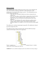
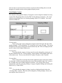
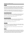
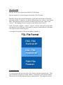
USER GUIDE for GRAPHICAL DATABASE for CATEGORY THEORY 3.0 Jeremy Bradbury, Ian Rutherford, Matthew Graves, Jesse Tweedle and Robert Rosebrugh February 2006 Table of Contents Section 1: Introduction – About GDCT – Development Team – Installation – Directory Structure Section 2: Categories and the File Menu – Introduction – Category File Types – CAT File Format – CGL File Format – Creating Categories – Opening Categories – Downloading Categories Section 3: Graphical Display of Categories – Introduction – Visual Display Controls – View GML – Saving Categories – Adding Data – Removing Data Section 4: Category Tools – Create Sum – Create Product – Coequalizer – Epimorphism – Equality of Composites – Equalizer – Initial Object – Isomorphism – Make Confluent – Make Dual Category – Monomorphism – Partial Order – Product – Pullback – Pushout – Sum – Terminal Object Section 5: Functors and the File Menu_ – Introduction _____ – – – – – – – – Functor File Types FUN File Format FGL File Format Creating Functors Opening Functors Downloading Functors Saving Functors Diagram Display Section 6: Settings – Category Graphical Settings – Server Settings – Endomorphism Limit Appendix A: Menu Item Shortcuts – List of Shortcuts Appendix B: Miscellaneous Information – Version Information – Bug Report Appendix C: File Format Examples User Guide for GDCT Section 1: Introduction________________________________ About GDCT Graphical Database for Category Theory was developed in the summers of 1999-2004 with funding from NSERC USRAs, NSERC Discovery grants and Mount Allison University. This application allows for the creation, editing, and storage of finitely presented categories. Categories can be opened and saved from local files as well as loaded from a specified server. Once a category file is in memory it can be tested for properties of objects and arrows. The tools available in this version of GDCT are listed in Section 4 of the Table of Contents. This program also allows the display of categories through the use of graph classes that were developed at Auburn University for Visualizing Graphs with Java (VGJ), a tool for graph drawing and graph layout. The original program was heavily modified for displaying categories. It can be found at http://www.eng.auburn.edu/department/cse/research/graphdrawing/. Functors between finitely presented categories can also be created and stored. Functors in memory display their domain and codomain categories, and their action is shown by an animated display. Some of the algorithms used in GDCT were originally developed in A Database of Categories, a C program written by Ryan Gunther and Michael Fleming with supervision by Robert Rosebrugh. This is available at http://mathcs.mta.ca/research/rosebrugh/dbc/. The GDCT application is developed from on Category Theory Database Tools, a Java applet written by Jeremy Bradbury with supervision by Robert Rosebrugh. This program is available at http://mathcs.mta.ca/research/rosebrugh/ctdt/. Development Team Installation The most current version of Graphical Database of Category Theory is available for download at http://mathcs.mta.ca/research/rosebrugh/gdct/downloadv30.htm. There are three installation options. The first option is available only to Windows 95/98/NT/2000/XP users. Options two and three are available to users of all platforms. Option One: Download Compiled Java Source Files and Java Runtime Environment [Windows Only] This includes source files compiled into a jar file. This setup includes a Java Runtime Environment for Windows 95/98/NT/2000/XP only. This version of the GDCT Setup is ~2 MB in size. Option Two: Download Compiled Java Source Files The option includes in the *.jar file and sample files, but does not include the JRE. This option will most likely be used by someone who wants to install GDCT under a Linux or Macintosh environment. Linux Instructions: You will need the latest JRE from http://java.sun.com. From the command prompt type “java -jar gdct.jar”. Macintosh Instructions: You will need to get the MRJ SDK from http://developer.apple.com/java/download/.html. Then run the program JBindery. Enter GDCT for the class name. Under the Class Path tab click “Add *.zip” and then select gdct.jar. This creates a double-clickable file that is equivalent to a Windows *.bat file. Option Three: Download Java Source Files and Java Developer's Kit The complete Java source files are available for download and may be modified under the terms of the GNU General Public License, Version 2. This download also includes all necessary help files as well as sample category and functor files. It is available as a *.zip file or as a *.tar.gz file. In order to compile and interpret Java source files, the Java Developers Kit must be downloaded. JDKs are used by an operating system to compile Java source files and interpret Java class files so they can be run on the local machine. Directory Structure Upon installation, the Graphical Database for Category Theory, unless changed by the user, will be installed in a directory called GDCT. Inside this directory are the subdirectories cat, cgl, fgl, fun, Help, Images, and Jre1.1. The following files are also located inside the main directory: – GDCT.bat: This is the batch file that the user selects to interpret the java archive (jar) – GDCT.jar: This is the java archive file that is interpreted by the Java Runtime Environment. This file contains all of the compiled Java source files. – GDCT.ico: This is an icon file that is used on any shortcuts to the GDCT application. – GDCT.ini: This initialization file contains information regarding internal settings, category graphical settings, functor graphical settings, functor animation settings, server settings, as well as a list of the most recently opened files. The subdirectories cat and cgl contain sample category files. The subdirectories fun and fgl contain sample functor files. The subdirectory Help contains all of the help files while the subdirectory Images contains all of the images used by the Java application. The Jre1.1 subdirectory contains the Java Runtime Environment Version 1.1 which is called by GDCT.bat to interpret the GDCT.jar. WARNING: The user should not modify any files in the subdirectories Help or Images. Section 2: Categories__________________________________ Introduction A finitely presented category can be considered a “directed graph with relations between paths of its edges.” Our notation for category data is: Objects: A, B, C, D, ... Maps/Arrows: e: AA, f:Ag:BC, h:AC... Identity Maps/Arrows: 1:AA, ... (one for each object) Composition of Maps/Arrows defined by Relations: e = 1, g*f = h, ... (path of arrows) NOTE: The identity Maps/Arrows are not explicitly stored or displayed but they are used and should not be added manually. File Types, Categories In GDCT, there are three different file types associated with categories: *.cat These files are a text only representation of a category. These files can be both opened and saved. Since a graphical representation of the category is not saved one is generated randomly upon opening the *.cat file. *.cgl These files contain both text and graphical representations of a category and can be both opened and saved. They are a concatenation of a .cat file and a .gml file. *.gml These files contain only a graphical representation of a category. These files can only be saved (and may be used by the VGJ applet), they cannot be opened. CAT File Format The text representation of categories is stored in the following format. Any line that is a comment must start with the “#” character. On the line following the word “category” is the category name. Objects are listed between the words “objects” and “arrows”. Arrows are listed between the words “arrows” and “relations.” Relations are listed after the word “relations.” NOTE: The words “category”, “objects”, “arrows”, relations”, and “gml” are key words and cannot be used as the name of the category or as the name of an object or arrow within the category. Objects and arrows can be a string of any length and can contain any ASCII characters excluding blank and “: - > * # . = ,” Relations are composed using the composition symbol “*”. An example of a typical CAT file can be found in Appendix C. CGL File Format A CGL file contains the information for both a text representation and a graphical representation. The text representation is the same as the file format for CAT files. Any line that is a comment must start with the “#” character. On the line following the word “category” is the category name. Objects are listed between the words “objects” and “arrows”. Arrows are listed between the words “arrows” and relations”. Relations are listed after the word “relations”. NOTE: The words “category”, “objects”, “arrows”, “relations”, and “gml” are key words and cannot be used as the name of the category or as the name of an object or arrow within the category. Objects and arrows can be a string of any length and can contain any ASCII characters excluding “: - > * # . = ,” Arrows are composed using the composition symbol “*”. The graphical representation uses a format known as gml which was developed at Auburn University for use with the Visualizing Graphs with Java (VGJ) project. It is incorporated into the cgl format by placing it at the end of the file after the keyword “gml”. For more information consult the VGJ Documentation. An example of a typical CGL file can be found in Appendix C. Creating Categories To create a category in memory the user selects File | New Category. The names of objects and arrows can be strings of any length except for reserved words and may contain any ASCII characters excluding “: - > * # . = ,” To add an object to the category, type the name of the object into the field labeled “Object (s):” and click “Add Object.” The object will appear in the table. To add an arrow to the category, type the name of the arrow into the field labeled “Arrow (s):”; then select a domain and codomain from the objects in the drop-down list; when finished, click “Add Arrow.” The arrow, domain and codomain will appear in the table. To add a relation, type in the equation, with composable arrows separated by the composition symbol “*” (e.g. f*g = h), then click “Add Relation”. NOTE: Only valid equations are accepted. An equation is invalid if it contains arrows that are not in the category, or an undefined composition, or if the domain and codomain of the left side do not equal the domain and codomain of the right side. Opening Categories In order to open a stored category file (.cgl or .cat) select File | Open Category. This opens a file selection window. If there is an error in the format of the selected file an error message is displayed and the open is aborted. Downloading Categories In order to download a category file (.cgl or .cat) select File | Download Category. This will display a list of categories. If the program cannot locate the files on the server an error message will be displayed. This could result from the user not being connected to the Internet or as a result of a server error. To change the settings for downloading categories, select Settings | Set Server. This displays a dialog for changing the default server and directories from which categories and functors can be downloaded. Saving Categories In order to save a category file select (in its category window) File | Save or File | Save As. The latter option opens a file selection window. Adding Data Selecting File | Add Data (in a category window) opens a dialog that allows the user to add information to the category Adding Objects: go to the “Objects” tab, type an object name into the field, then click “Add Object”. Adding Arrows: go to the “Arrows” tab, type an arrow name into the field, select a domain and codomain from the drop-down lists, and click “Add Arrow” Adding Relations: go to the “Relations” tab, type a valid relation into the field, and click add relation. Adding Comments: go to the “Comments” tab, type comments directly in the text area. If the input is correct, the added attribute will appear immediately in the appropriate text area. You may also change the category name; when finished, click “Done”. If the changes are not acceptable to you, click “Cancel”. Removing Data To remove data from a category, the user selects any and all attributes to remove, and then clicks “Cancel”. If there are any problems with the removal, the details will be listed in the text area below. When removal is complete, the user may click “Close” to implement the changes, or “Cancel” to cancel them. Section 3: Graphical Display of Categories______________ Introduction The controls for the graphical display of categories are explained under the title “Visual Display Controls”. This section deals with manipulating the graphical display of a category. There are two ways to select an object or arrow. The first is to click directly on the object or arrow so that it becomes highlighted red. The second way is to click and hold the left mouse button down before dragging a square around the desired object(s) or arrow(s). Once an object or arrow has been selected, it can be moved by holding down on it and dragging it to another position on the graphical display canvas. Visual Display Controls The controls for the graphical display of categories were developed at Auburn University as part of the 3D package that is used by GDCT in the display of categories. The visual controls can be hidden from view selecting Settings | Show VGJ Controls. The visual controls available are: Viewing Angles The viewing angle can be changed by using the control below the left side of the graphical display. Click and hold the “X” to rotate the view to any 3D angle. The current orientation of the category displayed can be determined by the XYZ axis displayed in the top left corner of the category display area. Viewing Plane The plane that the category is being viewed in can be changed by pressing one of the three buttons below the “Viewing Angles” control window in the bottom right corner of the main screen. The user can select the XY plane, XZ plane, or the YZ plane. Viewing Offset The viewing offset is located in the bottom right hand corner of the main window. It is basically a virtual screen that allows the user to click and hold on the “box” to move the viewable canvas area without using the scroll bars. The viewing offset can be automatically centred by selecting Settings | Category Graphical Settings and clicking the check box by “Center Offset”. Zoom The scale that the category is being viewed at is displayed directly below the “Viewing Offset” controls. The scale can be changed by clicking Settings | Zoom, and selecting the desired zoom level. View GML GML is the text representation of the graphical display of the current category. To view the GML code select Settings | View GML. Choosing this menu option will display a frame containing the GML code. Each object is stored as a node. The relations are stored as a single node. The arrows are stored as edges between nodes. Multiple arrows between objects are stored as one edge with commas separating the names of individual arrows. Section 4: Category Tools______________________________ Coequalizer In a category window, selecting Tools | Coequalizer? opens a dialog window allowing the specification of a first and second paths, and then a path to be tested as a coequalizer of the two paths. The "Coequalizer object" checkbox may be checked allowing either selection of a possible coequalizer object from a drop-down list or the user may choose to check all objects. All paths to the object (or objects) will then be tested as coequalizers. WARNING: The domain and codomain of the two paths must be the same. The codomain of the two paths must be the same as the domain of the coequalizer path. The test is only valid on a confluent category. (If in doubt use the Make Confluent tool). Create A Product Of Categories Selecting (in a Category window) Tools | Create Product opens a dialog which allows the user to create a product of categories; select another category from the drop-down list, and click "OK". This will open a new window containing the product category. NOTE: To save the product category, select File | Save As. Create A Sum Of Categories Selecting (in a Category window) Tools | Create Sum opens a dialog which allows the user to create a sum of categories; select another category from the drop-down list, and click "OK". This will open a new window containing the sum category. NOTE: To save the sum category, select File | Save As. Epimorphism In a category window, selecting Tools | Epimorphism? opens a dialog window allowing input of a path to check as an epimorphism. Additionally, the "Check all paths" checkbox may be selected to check all paths in the current category. WARNING: The test is only valid on a confluent category. (If in doubt use the Make Confluent tool). Equalizer In a category window, selecting Tools | Equalizer? opens a dialog window allowing the specification of a first and second paths, and then a path to be tested as an equalizer of the two paths. The "Equalizer object" checkbox may be checked allowing either selection of a possible equalizer object from a drop-down list or the user may choose to check all objects. All paths from the object (or objects) will then be tested as equalizers. WARNING: The domain and codomain of the two paths must be the same. The domain of the two paths must be the same as the codomain of the equalizer path. The test is only valid on a confluent category. (If in doubt use the Make Confluent tool). Equality of Composites To test two (composite) arrows for equality in the current category select (in a category window) Tools | Equality of Composites. A dialog allows entry of two paths. WARNING: The category must be confluent for valid results. Domains and codomains of paths must match. Initial Object In a category window, select Tools | Initial Object?. This command tests objects of the current category (chosen by a dialog) for initiality. For each selected object which is not initial a reason is given. WARNING: This command will not operate correctly unless the category has a confluent set of relations. If in doubt use Make Confluent tool first. Isomorphism In a category window, selecting Tools | Isomorphism? opens a dialog window allowing the input of up to non-identity two paths to be checked for isomorphism. Additionally, the "Check all paths" checkbox may be selected to check all paths of the current category. WARNING: The test is only valid on a confluent category. (If in doubt use the Make Confluent tool). Make Confluent In a category window, select Tools | Make Confluent. This command applies the KnuthBendix algorithm to the currently displayed category with arrows ordered in their storage order. Relations which are added to the current category are reported. To add these relations to the current category click "Ok", or click "Cancel" to keep the category in its current form. Make Dual This tool will create the opposite category of the currently displayed category. In a category window, select Tools | Make Dual. A dialog window opens prompting for the name of the dual. After the user provides the name the dual category is displayed in a new window. WARNING: The opposite category is NOT SAVED automatically when it is created; use (in the category window) File | Save if you wish to save the dual. Monomorphism In a category window, selecting Tools | Monomorphism? opens a dialog window allowing input of a path to check as a monomorphism. Additionally, the "Check all paths" checkbox may be selected to check all paths in the current category. WARNING: The test is only valid on a confluent category. (If in doubt use the Make Confluent tool). Partial Order To test if a category is a partial order, select (in a category window) Tools | Partial Order. WARNING: The category must be confluent for valid results. Product In a category window, selecting Tools | Product? opens a dialog window allowing selection of a possible product object from the current category from a drop-down and specification of (possibly composite) first and second projections, then testing the span for being a product. If `Check all objects' is selected, then enter two objects in order to check all spans to the two objects for being a product. WARNING: The domain of each projection must be the putative product object. The test is only valid on a confluent category. (If in doubt use the Make Confluent tool). Pullback In a category window, selecting Tools | Pullback? opens a dialog window allowing selection of a possible pullback object from the current category from a drop-down and specification of (possibly composite) paths alpha and beta forming a cospan (and optionally projections), then testing for pullback(s). WARNING: The test is only valid on a confluent category. (If in doubt use the Make Confluent tool). Pushout In a category window, selecting Tools | Pushout? opens a dialog window allowing selection of a possible pushout object from the current category from a drop-down and specification of (possibly composite) paths alpha and beta forming a span (and optionally co-projections), then testing for pushout(s). WARNING: The test is only valid on a confluent category. (If in doubt use the Make Confluent tool). Sum In a category window, selecting Tools | Sum? opens a dialog window allowing selection of a possible sum object from the current category from a drop-down and specification of (possibly composite) first and second injections, then testing the cospan for being a sum. If `Check all objects' is selected, then enter two objects in order to check all cospans from the two objects for being a sum. WARNING: The codomain of each injection must be the putative sum object. The test is only valid on a confluent category. (If in doubt use the Make Confluent tool). Terminal Object In a category window, select Tools | Terminal Object?. This command tests objects of the current category (chosen by a dialog) for being terminal. For each selected object which is not terminal a reason is given. WARNING: This command will not operate correctly unless the category has a confluent set of relations. If in doubt use Make Confluent Tool first. Section 5: Functors___________________________________ Introduction A functor is a “structure preserving” interpretation of one finitely presented category into another. A functor preserves the structure of a category because it sends: Objects to Objects Arrows to Arrows and it preserves the composition that is provided by relations. Functor File Types In GDCT there are two different file types that are associated with functors. *.fun These files are a text only representation of a functor. These files can be both opened and saved. Since a graphical representation of the two categories involved is not saved, the graphical representations are generated randomly upon opening the *.fun file. *.fgl These files contain both a text and graphical representation of the categories involved in a given functor as well as the functor information itself. This type of file can be both opened and saved. FUN File Format The text representation of functors is stored in the following three part format. Part one consists of a category stored in the CAT file format. Part two consists of a second category stored in the CAT file format. Part three consists of the functor information. In this part, any line that is a comment must start with the “#” character. On the line following the word “functor” is the functor name. The mapping of objects to objects is listed between the words “objects” and “arrows”. The mapping of arrows to paths is listed after the word “arrows”. NOTE: The words “category”, “functor”, “objects”, “arrows”, and “gml” are key words and cannot be used as the name of the categories, functors between them or as the name of an object or arrow within categories. An example of a typical FUN file can be found in Appendix C. FGL File Format Part one consists of a category stored in the CGL file format. Part two consists of a second category stored in the CGL file format. Part three consists of the functor information. In this part, any line that is a comment must start with the “#” character. On the line following the word “functor” is the functor name. The mapping of objects to objects is listed between the words “objects” and “arrows”. The mapping of arrows to paths is listed after the word “arrows”. NOTE: The words “category”, “functor”, “objects”, “arrows”, and “gml” are key words and cannot be used as the name of the categories, functors between them or as the name of an object or arrow within categories. An example of a typical FGL file can be found in Appendix A. Creating Functors To create a functor the user selects File | New Functor, and enter a functor name. Then select the domain category by clicking “Browse”, which opens a file selection window. Then do the same for the codomain category, and click Next. This opens the selected categories to enable the user to easily choose mappings for the functor. Select an object in the “Domain” list (i.e. an object from the domain category) and its corresponding object in the “Codomain” list. Continue until all domain objects are gone. Then you will need to choose the arrow mappings; first select an arrow from the domain category, then input a codomain path of composable arrows and click “Add Mapping”. Click “Done” when finished, and the functor will be displayed. The name of the functor can be a string of any length except for reserved words and may contain any ASCII characters excluding “: - > * # . = ,” Opening Functors In order to open a stored functor file (.fun or .fgl)) select File | Open Functor. If there is any error in the format of the selected file an error message is displayed and the open is aborted. Downloading Functors In order to download a functor file (.fun or .fgl) select File | Download Functor. The functors listed are located on the server specified in the frame's title bar. To select a functor to download simply double click on the functor's name of click once on the functor name and press the OK button. Either of these methods will display the downloaded functor. If the program cannot locate the files on the server an error message will be displayed. This could result from the user not being connected to the Internet or as a result of a server error. To change the settings for downloading functors, select Settings | Set Server. This displays a dialog for changing the default server and directories from which categories and functors can be loaded using the appropriate load command. Saving Functors In order to save a functor in memory select File | Save or File | Save As. Diagram Display Functors can also be viewed as diagrams, with the graphical display taken from the domain category and the object and arrow names taken from the codomain category. To view a functor as a diagram, click the “Diagram Display” button in the top left corner when a functor is open. To switch back to normal functor display mode, click the “Two Category Display” button. NOTE: When first opened, a functor's diagram display has a newly created graph with object positions taken from the domain category. A diagram graph is NOT saved in either functor file format. Section 6: Settings____________________________________ Category Graphical Settings Selecting Settings | Zoom in a category window allows the user to zoom in and out of the displayed graph. Selecting Settings | Show VGJ Controls allows to user to toggle the VGJ controls at the bottom of the window. Selecting Settings | View GML allows the user to view the GML for the category. Server Settings Selecting Settings | Set Server in the main window displays a dialog for changing the default server and directories from which categories and functors can be loaded using the appropriate load command. Endomorphism Limit Selecting Settings | Endomorphism Limit in the main window displays a dialog for changing the endomorphism limit. The endomorphism limit is a check built into many tools to alert the user to a possible inaccuracy of the results; if the endomorphism limit is passed (there are too many loops in the category), a warning is issued with the results of the tool. Appendix A: Menu Item Shortcuts_______________________ The following shortcuts to menu items are supported in GDCT. ALT+F: File Menu ALT+N: New Category ALT+O: Open Category ALT+D: Download Category ALT+F: Download Functor ALT+X: Exit Program ALT+S: Settings Menu ALT+S: Server Settings ALT+E: Endomorphism Limit ALT+W: Window Menu ALT+C: Close All Windows ALT+H: Help Menu ALT+H: Help Topics Index ALT+B: Bug Report ALT+G: About GDCT ALT+A: About Authors Appendix B: Miscellaneous Information_________________ Version Information The Graphical Database for Category Theory is a research project at Mount Allison University that now includes over 70 Java source files and over 30000 lines of code. Version 1.0: Released March 20, 2000 This is the preliminary version of Graphical Database for Category Theory Version 1.1: Released Summer 2000 This version of GDCT contained fixes and enhancements described in its user guide. See: http://mathcs.mta.ca/research/rosebrugh/gdct/v1release.htm Version 2.0: Released May 2002 This version of GDCT contained fixes and enhancements described in its user guide. See: http://mathcs.mta.ca/research/rosebrugh/gdct/gdct2.0/index.html Version 3.0: Released February 2006/Alpha This version of GDCT contained the following fixes and enhancements: – Moved to a desktop-style interface, where multiple categories and functors can be opened in their own respective windows – Completely removed Borland from the software. – Converted most graphic components from AWT to Swing (lightweight) – Divided each tool into two separate classes: an interface class and an algorithm class – Implemented pullback, pushout, create product, create sum, and partial order category tools. – Converted most lingering C based code to object oriented. Appendix C: File Format Examples_______________________ An example .cat file: #a commutative triangle category triangle.cat objects A, B, C. arrows ab:A->B, ac:A->C, bc:B->C. relations bc*ab = ac. An example .cgl file: # A parallel pair plus equalizing arrow. category equalizer.cgl objects A, B, C. arrows f:B->A, g:B->A, h:C->B. relations g*h = f*h. gml graph [ directed 1 node [ id 0 label "A" graphics [ Image [ Type "" Location "" ] center [ x 125.0 y -1.0 z 0.0 ] width 15.94 height 28.72 depth 20.0 ] vgj [ color "black" labelPosition "in" shape "Oval" ] ] node [ id 1 label "B" graphics [ Image [ Type "" Location "" ] center [ x 2.0 y -1.0 z 0.0 ] width 17.36 height 28.72 depth 20.0 ] vgj [ color "black" labelPosition "in" shape "Oval" ] ] ] node [ id 2 label "C" graphics [ Image [ Type "" Location "" ] center [ x -101.0 y -1.0 z 0.0 ] width 18.78 height 28.72 depth 20.0 ] vgj [ color "black" labelPosition "in" shape "Oval" ] ] node [ id 3 label "relations\nf*h = g*h" graphics [ Image [ Type "" Location "" ] center [ x 0.0 y -150.0 z 0.0 ] width 74.16 height 51.44 depth 20.0 ] vgj [ color "black" labelPosition "in" shape "Oval" ] ] edge [ linestyle "solid" label "h" source 2 target 1 ] edge [ linestyle "solid" label "g,f" source 1 target 0 ] An example .fun file: category csquare objects A, B, C, D. arrows f:A->B, g:A->C, h:B->D, k:C->D. relations k*g = h*f. category coequalize objects A, B, C. arrows f:A->B, g:A->B, h:B->C. relations h*g = h*f. functor cscoeq objects A |--> A, B |--> B, C |--> B, D |--> C. arrows f |--> f, g |--> g, h |--> h, k |--> h. An example .fgl file: #skeleton of sets with 3 or less elements category parpair objects A, B. arrows f:A->B, g:A->B. relations . gml graph [ directed 1 node [ id 0 label "A" graphics [ Image [ Type "" Location "" ] center [ x -144.0 y 11.0 z 0.0 ] width 15.94 height 27.299999999999997 depth 20.0 ] vgj [ labelPosition "in" shape "Oval" ] ] ] node [ id 1 label "B" graphics [ Image [ Type "" Location "" ] center [ x 121.0 y 13.0 z 0.0 ] width 17.36 height 27.299999999999997 depth 20.0 ] vgj [ labelPosition "in" shape "Oval" ] ] edge [ linestyle "solid" label "g,f" source 0 target 1 ] #skeleton of sets with 3 or less elements category set3 objects 0, 1, 2, 3. arrows d00:0->1, d10:1->2, d11:1->2, e00:2->1, d20:2->3, d21:2->3, d22:2->3, e10:3->2, e11:3->2, s00:2->2, s10:3->3, s11:3->3. relations e00*d10 = 1, e00*d11 = 1, d11*d00 = d10*d00, d21*d10 = d20*d10, d22*d10 = d20*d11, d22*d11 = d21*d11, e00*e11 = e00*e10, e11*d20 = d10*e00, e10*d20 = 1, e11*d21 = 1, e10*d21 = 1, e11*d22 = 1, e10*d22 = d11*e00, s00*s00 = 1, s00*d10 = d11, s10*d22 = d22*s00, s10*d20 = d21, s11*d21 = d22, s11*d20 = d20*s00, e11*s10*s11 = s00*e10, e10*s10 = e10, e11*s11 = e11, e00*s00 = e00, s11*s11 = 1, s10*s10 = 1, s10*d21 = d20, s11*d22 = d21, s00*d11 = d10, e10*s11*s10 = s00*e11, s11*s10*s11 = s10*s11*s10, e00*e10*s11 = e00*e10, s00*e10*s11 = e11*s10, s00*e11*s10 = e10*s11, d22*d10*d00 = d20*d10*d00, s11*d20*d10 = d22*d10, s10*d22*d10 = d21*d11, e11*s10*d22 = s00, s11*s10*d22 = d21*s00, e10*s11*d20 = s00, s10*s11*d20 = d21*s00, s10*d22*e10*s11 = d22*e11*s10, s11*d20*e10*s11 = d20*e11*s10, s10*d22*e11*s10 = d22*e10*s11, s11*d20*e11*s10 = d20*e10*s11. gml graph [ directed 1 node [ id 0 label "0" graphics [ Image [ Type "" Location "" ] center [ x -199.0 y 0.0 z 0.0 ] width 15.94 height 27.299999999999997 depth 20.0 ] vgj [ labelPosition "in" shape "Oval" ] ] node [ id 1 label "1" graphics [ Image [ Type "" Location "" ] center [ x -100.0 y 0.0 z 0.0 ] width 15.94 height 27.299999999999997 depth 20.0 ] vgj [ labelPosition "in" shape "Oval" ] ] node [ id 2 label "2" graphics [ Image [ Type "" Location "" ] center [ x 50.0 y 0.0 z 0.0 ] width 15.94 height 27.299999999999997 depth 20.0 ] vgj [ labelPosition "in" shape "Oval" ] ] node [ id 3 label "3" graphics [ Image [ Type "" Location "" ] center [ x 220.0 y 0.0 z 0.0 ] width 15.94 height 27.299999999999997 depth 20.0 ] vgj [ labelPosition "in" shape "Oval" ] ] node [ id 4 label "relations\ne00*d10 = 1,e00*d11 = 1,d11*d00 = d10*d00,d21*d10 = d20*d10,d22*d10 = d20*d11,\nd22*d11 = d21*d11,e00*e11 = e00*e10,e11*d20 = d10*e00,e10*d20 = 1,e11*d21 = 1,\ne10*d21 = 1,e11*d22 = 1,e10*d22 = d11*e00,s00*s00 = 1,s00*d10 = d11,\ns10*d22 = d22*s00,s10*d20 = d21,s11*d21 = d22,s11*d20 = d20*s00,e11*s10*s11 = s00*e10,\ne10*s10 = e10,e11*s11 = e11,e00*s00 = e00,s11*s11 = 1,s10*s10 = 1,\ns10*d21 = d20,s11*d22 = d21,s00*d11 = d10,e10*s11*s10 = s00*e11,s11*s10*s11 = s10*s11*s10,\ne00*e10*s11 = e00*e10,s00*e10*s11 = e11*s10,s00*e11*s10 = e10*s11,d22*d10*d00 = d20*d10*d00,s11*d20*d10 = d22*d10,\ns10*d22*d10 = d21*d11,e11*s10*d22 = s00,s11*s10*d22 = d21*s00,e10*s11*d20 = s00,s10*s11*d20 = d21*s00,\ns10*d22*e10*s11 = d22*e11*s10,s11*d20*e10*s11 = d20*e11*s10,s10*d22*e11*s10 = d22*e10*s11,s11*d20*e11*s10 = d20*e10*s11" graphics [ Image [ Type "" Location "" ] center [ x 0.0 y -133.0 z 0.0 ] width 1069.58 height 219.0 depth 20.0 ] vgj [ labelPosition "in" shape "Oval" ] ] edge [ linestyle "solid" label "d22,d20,d21" source 2 target 3 ] ] edge [ linestyle "solid" label "s11,s10" source 3 target 3 ] edge [ linestyle "solid" label "d11,d10" source 1 target 2 ] edge [ linestyle "solid" label "e11,e10" source 3 target 2 ] edge [ linestyle "solid" label "s00" source 2 target 2 ] edge [ linestyle "solid" label "d00" source 0 target 1 ] edge [ linestyle "solid" label "e00" source 2 target 1 ] functor pp2s3 objects A |--> 1, B |--> 2. arrows f |--> d11, g |--> d10.