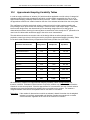
1
Microdata User Guide The Canadian Survey of Experiences with Primary Health Care 2007-2008 The Canadian Survey of Experiences with Primary Health Care, 2007-2008 – User Guide Table of Contents 1.0 Introduction ............................................................................................................................... 5 2.0 Background ............................................................................................................................... 7 3.0 Objectives ............................................................................................................................... 9 4.0 Concepts and Definitions............................................................................................................ 11 5.0 Survey Methodology.................................................................................................................... 13 5.1 Canadian Community Health Survey Population Coverage ............................................. 13 5.2 Canadian Community Health Survey Sample Design ...................................................... 13 5.3 The Canadian Survey of Experiences with Primary Health Care Population Coverage .. 13 5.4 Person Sampling Strategy and Sample Size.................................................................... 14 6.0 Data Collection ............................................................................................................................. 15 6.1 Questionnaire Design ....................................................................................................... 16 6.2 Supervision and Quality Control ....................................................................................... 16 7.0 Data Processing ........................................................................................................................... 17 7.1 Data Capture..................................................................................................................... 17 7.2 Editing ............................................................................................................................. 17 7.3 Coding of Open-ended Questions .................................................................................... 17 7.4 Imputation ......................................................................................................................... 17 7.5 Creation of Derived Variables ........................................................................................... 18 7.6 Weighting .......................................................................................................................... 18 7.7 Suppression of Confidential Information........................................................................... 18 8.0 Data Quality ............................................................................................................................. 21 8.1 Response Rates................................................................................................................ 21 8.2 Survey Errors .................................................................................................................... 21 8.2.1 The Frame............................................................................................................ 22 8.2.2 Data Collection..................................................................................................... 22 8.2.3 Non-response....................................................................................................... 22 8.2.4 Measurement of Sampling Error .......................................................................... 22 9.0 Guidelines for Tabulation, Analysis and Release..................................................................... 25 9.1 Rounding Guidelines......................................................................................................... 25 9.2 Sample Weighting Guidelines for Tabulation.................................................................... 25 9.3 Definitions of Types of Estimates: Categorical and Quantitative...................................... 26 9.3.1 Categorical Estimates .......................................................................................... 26 9.3.2 Quantitative Estimates ......................................................................................... 26 9.3.3 Tabulation of Categorical Estimates .................................................................... 27 9.3.4 Tabulation of Quantitative Estimates ................................................................... 27 9.4 Guidelines for Statistical Analysis ..................................................................................... 27 9.5 Coefficient of Variation Release Guidelines ..................................................................... 28 9.6 Release Cut-off’s for The Canadian Survey of Experiences with Primary Health Care ... 30 Special Surveys Division 3 The Canadian Survey of Experiences with Primary Health Care, 2007-2008 – User Guide 10.0 Approximate Sampling Variability Tables ................................................................................. 31 10.1 How to Use the Coefficient of Variation Tables for Categorical Estimates....................... 32 10.1.1 Examples of Using the Coefficient of Variation Tables for Categorical Estimates ............................................................................................................. 33 10.2 How to Use the Coefficient of Variation Tables to Obtain Confidence Limits................... 39 10.2.1 Example of Using the Coefficient of Variation Tables to Obtain Confidence Limits.................................................................................................................... 40 10.3 How to Use the Coefficient of Variation Tables to Do a T-test ......................................... 41 10.3.1 Example of Using the Coefficient of Variation Tables to Do a T-test................... 41 10.4 Coefficients of Variation for Quantitative Estimates.......................................................... 41 10.5 Coefficient of Variation Tables .......................................................................................... 42 10.6 Bootstrap Method for Variance Estimation ....................................................................... 42 10.7 Statistical Packages for Variance Estimation ................................................................... 43 10.7.1 Other Packages ................................................................................................... 43 11.0 Weighting ............................................................................................................................. 47 11.1 Weighting Procedures for the Canadian Community Health Survey................................ 47 11.2 Weighting Procedures for The Canadian Survey of Experiences with Primary Health Care ............................................................................................................................. 47 12.0 Questionnaires ............................................................................................................................. 51 13.0 Record Layout with Univariate Frequencies ............................................................................. 53 4 Special Surveys Division The Canadian Survey of Experiences with Primary Health Care, 2007-2008 – User Guide 1.0 Introduction The Canadian Survey of Experiences with Primary Health Care (CSE-PHC) was conducted by Statistics Canada from April to June 2008 with the cooperation and support of the Canadian Institute for Health Information and the Health Council of Canada. This manual has been produced to facilitate the manipulation of the microdata file containing the survey results. Any question about the data set or its use should be directed to: Statistics Canada Client Services Special Surveys Division Telephone: 613-951-3321 or call toll-free 1-800-461-9050 Fax: 613-951-4527 E-mail: [email protected] Special Surveys Division 5 The Canadian Survey of Experiences with Primary Health Care, 2007-2008 – User Guide 2.0 Background Special Surveys Division was originally contacted by the Health Council of Canada (HCC) during the summer of 2006 to conduct the first iteration of this survey which resulted in the Canadian Survey of Experiences with Primary Health Care (CSE-PHC), 2006-2007 survey. The HCC was created when the First Ministers' Accord on Health Care Renewal was signed in 2003. Their mandate is to report publicly on the progress of health care renewal in Canada. One of the Council’s goals is to provide a system-wide perspective on health care reform to the Canadian public with a particular focus on issues related to accountability and transparency. Once the results of the 2006-2007 survey were released, work began on the 2007-2008 questionnaire. The Canadian Institute for Health Information (CIHI) joined members of the HCC and the project team at Statistics Canada to begin shaping the 2007-2008 survey. The CIHI, which became a co-sponsor with the HCC, is an independent, national, not-for-profit organization working to improve the health of Canadians and the health care system by providing quality, reliable and timely health information. The research information they produce focuses on health care services, health spending and human resources working in the health sector, as well as issues surrounding the health of the population. The 2007-2008 survey differed from the 2006-2007 version in several ways. Along with some content changes, mostly around barriers to access and use of health care, the survey sample was expanded and a sampling strategy was developed to permit national as well as provincial level estimates of survey results. A new questionnaire was developed and tested with focus groups during the month of January 2008, in four cities across the country. The collection mode was also changed from a paper/pencil survey collected over the telephone in 2006-2007 to a computer-assisted telephone interview (CATI) application in 2007-2008. Collection began in three Statistics Canada regional offices in April and continued until the end of June 2008. Special Surveys Division 7 The Canadian Survey of Experiences with Primary Health Care, 2007-2008 – User Guide 3.0 Objectives The main objectives of the survey are to collect data on issues relating to experiences with health care that impact Canadians and to produce national and provincial estimates. More specifically, the goal was to provide a picture of access and utilization of primary care as well as information on issues specific to Canadians living with chronic conditions and their experiences with the health care system. Ultimately, the data collected will provide information for the development of effective policies and strategies, both provincially and nationally, to help improve health care for all Canadians. The data from this survey will provide a holistic perspective of Canadians’ experiences with health care while identifying and raising awareness around issues that affect people living with chronic conditions. Finally, one of the ultimate goals of the survey is to help in decision-making about resources and provide baseline data to monitor change over time. Special Surveys Division 9 The Canadian Survey of Experiences with Primary Health Care, 2007-2008 – User Guide 4.0 Concepts and Definitions Since the Canadian Survey of Experiences with Primary Health Care is conducted over the telephone, an effort was made to use simple terminology throughout the questionnaire in order to minimize long complicated explanations of survey concepts. Some standard concepts and definitions should be used in the analysis and interpretation of this data. The survey questions were designed with these definitions in mind. Primary Health Care refers to the main source of preventive as well as on-going or essential care people receive in their communities. They include regular medical doctors and family clinics. Often, this is the patient’s first contact with the health care system. Doctors are defined as medical doctors paid by provincial Medicare. All non medical doctors and those not covered under provincial Medicare systems were excluded. Special Surveys Division 11 The Canadian Survey of Experiences with Primary Health Care, 2007-2008 – User Guide 5.0 Survey Methodology The 2007-2008 Canadian Survey of Experiences with Primary Health Care (CSE-PHC) was administered from April 14 to June 30, 2008, to a sub-sample of the people who participated in the Canadian Community Health Survey (CCHS) Cycle 4.1 between July and December, 2007. Therefore its sample design is closely tied to that of the CCHS. The CCHS Cycle 4.1 design is briefly described in the Sections 5.1 to 5.2. 1 Sections 5.3 and 5.4 describe how the CSE-PHC departed from the basic CCHS Cycle 4.1 design. 5.1 Canadian Community Health Survey Population Coverage The CCHS data is collected from people aged 12 years and over living in private dwellings within the 10 provinces and three territories. Specifically excluded from the survey’s coverage are residents of Indian Reserves and Crown land, full-time members of the Canadian Armed Forces, inmates of institutions and residents of isolated areas. The CCHS represents approximately 98% of the Canadian population aged 12 years and over. 5.2 Canadian Community Health Survey Sample Design To provide reliable estimates to the 121 health regions (HR), a sample of 65,000 respondents is required on an annual basis. A multi-stage sample allocation strategy gives relatively equal importance to the HRs and the provinces. In the first step, the sample is allocated among the provinces according to the size of their respective populations and the number of HRs they contained. Each province's sample is then allocated among its HRs proportionally to the square root of the population in each HR. The CCHS uses three sampling frames to select the sample of households: 49% of the sampled households comes from an area frame, 50% comes from a list frame of telephone numbers and the remaining 1% comes from a Random Digit Dialling (RDD) telephone number frame. For most of the health regions, 50% of the sample is selected from the area frame and 50% from the list frame of telephone numbers. In two health regions (Nord-du-Québec and Prairie North), only the RDD frame is used. In Nunavut, only the area frame is used. In the Yukon and Northwest Territories, most of the sample comes from the area frame but a small RDD sample is also selected in the territorial capitals. The CCHS uses the area frame designed for the Labour Force Survey (LFS) as its area frame. Thus, the sampling plan of the LFS must be considered in selecting the CCHS dwelling sample. The LFS plan is a complex two stage stratified design in which each stratum is formed of clusters. The LFS first selects clusters using a sampling method with a probability proportional to size (PPS), and then the final sample is chosen using a systematic sampling of dwellings in the cluster. The CCHS uses the LFS clusters, which it then stratifies by HRs. Lastly, it selects a sample of clusters and dwellings in each HR. 5.3 The Canadian Survey of Experiences with Primary Health Care Population Coverage The target population for the 2007-2008 CSE-PHC is defined in the same way as for the CCHS Cycle 4.1, except that it is limited to people aged 18 and over on April 14, 2008. In addition, because the CSE-PHC is intended to represent the population of Canada at the beginning of 2008 but its sample is selected from the CCHS Cycle 4.1 respondents, who were interviewed between July and December 2007, people who joined the target population between the two surveys are excluded. This does not affect people who were not yet 18 at the time of the CCHS Cycle 4.1, since the latter included people aged 12 and over. 1 For a detailed description of the CCHS Cycle 4.1 sample design see the Public Use Microdata File guide, Catalogue no. 82M0013GPE. Special Surveys Division 13 The Canadian Survey of Experiences with Primary Health Care, 2007-2008 – User Guide 5.4 Person Sampling Strategy and Sample Size The 2007-2008 CSE-PHC was designed to produce provincial as well as national estimates of key health variables. Most of the respondents from the CCHS Cycle 4.1 sample collected between July and December 2007 (September and December for Ontario) was used. Almost the entire available sample was used in six of the 10 provinces (Newfoundland and Labrador, New Brunswick, Nova Scotia, Prince Edward Island, Manitoba and Saskatchewan) in order to maximize the minimum estimable proportion (min p ) of some very small variables of interest. Otherwise the target of a 7% min p was used in order to determine the sample size in the four provinces where extra sample was available. The sample was drawn systematically within each province of the population aged 18 and over. The sampling fraction is smaller in some of the larger provinces, specifically in Ontario and Quebec. In these provinces the design effects are larger; however the larger sample size in these areas compensates to minimize the impact. A very small sample of 100 units was created for the Territories. These units were selected systematically and proportionally across the Yukon, Northwest Territories and Nunavut in order to produce national estimates only. The sample size of the CSE-PHC is 16,482 persons. The table below shows the number of persons sampled in each province and territory. Provinces and Territories Newfoundland and Labrador 971 Prince Edward Island 671 Nova Scotia 1,258 New Brunswick 1,285 Quebec 2,300 Ontario 2,345 Manitoba 1,723 Saskatchewan 1,675 Alberta 2,300 British Columbia 1,854 Territories Canada 14 Sample Size 100 16,482 Special Surveys Division The Canadian Survey of Experiences with Primary Health Care, 2007-2008 – User Guide 6.0 Data Collection An introductory letter was mailed to respondents approximately one week before data collection began. Collection for the 2007-2008 Canadian Survey of Experiences with Primary Health Care (CSEPHC) was carried out from mid-April to the end of June, 2008 and was done using a computerassisted telephone interviewing (CATI) application. The CATI system has a number of generic modules which can be quickly adapted to most types of surveys. A front-end module contains a set of standard response codes for dealing with all possible call outcomes, as well as the associated scripts to be read by the interviewers. A standard approach set up for introducing the agency, the name and purpose of the survey, the survey sponsors, how the survey results will be used, and the duration of the interview was used. We explained to respondents how they were selected for the survey, that their participation in the survey is voluntary, and that their information will remain strictly confidential. Help screens were provided to the interviewers to assist them in answering questions that are commonly asked by respondents. The CATI application ensured that only valid question responses were entered and that all the correct flows were followed. Edits were built into the application to check the consistency of responses, identify and correct outliers, and to control who gets asked specific questions. This meant that the data was already quite “clean” at the end of the collection process. The survey manager met with senior staff responsible for collection to discuss issues and questions before the start of the training session. A description of the background and objectives as well as a detailed description of concepts and definitions particular to the 2007-2008 CSE-PHC was provided for interviewers in their Interviewer Manual. A glossary of terms and a set of questions and answers were also included. Interviewers were trained on the survey content through a classroom training session. In addition, the interviewers completed a series of mock interviews to become familiar with the survey, its concepts, definitions and the CATI application itself. Question and answer documentation was provided to the interviewers to assist them in answering questions that are commonly asked by respondents. The data collection was conducted by specialized staff at Statistics Canada offices in Edmonton, Sturgeon Falls and Sherbrooke. The workload and interviewing staff within each office was managed by a project manager. The automated scheduler used by the CATI system ensured that cases were assigned randomly to interviewers and that cases were called at different times of the day and different days of the week to maximize the probability of contact. There were a maximum of 20 call attempts per case identified as a residential phone number; once the maximum was reached, the case was reviewed by a senior interviewer who determined if additional calls would be made. There were a maximum of 5 call attempts per case identified as an unknown phone number; if during these 5 call attempts a phone number was identified as belonging to a household the maximum was raised to 20. The average interview time was estimated to be 22 minutes. However, the length of the interviews varied depending on the circumstances of the respondent. For example, the average interview time was estimated to be 30 minutes for a respondent with chronic conditions and 12 minutes for those without chronic conditions. There was no tracing of respondents, for those that moved between the time they completed the Canadian Community Health Survey (CCHS) and the time they were contacted for the 2007-2008 CSE-PHC. However, the CCHS captures alternate contact information for tracing respondents which proved to be very successful in locating people that had moved. Special Surveys Division 15 The Canadian Survey of Experiences with Primary Health Care, 2007-2008 – User Guide 6.1 Questionnaire Design The Health Council of Canada (HCC) and the Canadian Institute for Health Information (CIHI) provided input into the development of the draft questionnaire, this included mapping to 27 health indicators developed by CIHI. A new version of the questionnaire was created to reflect the research goals, objectives and indicators of the co-sponsors. The length was dramatically reduced and the flow of the interview was improved. The redesign questionnaire was translated by Official Languages and Translation Division and tested in conjunction with Environics Research Group using face to face interviews in both official languages in four Canadian cities. The testing was conducted with respondents from various age groups and ethnic backgrounds. A portion of the test group was comprised of people diagnosed with chronic conditions. Further changes to the questionnaire were implemented based on the results of the questionnaire testing process. Once a final version of the questionnaire was decided on, specifications were drawn up and a CATI application was developed and tested. Specifications for valid ranges and interquestion consistency were incorporated into the CATI application to the extent feasible. After extensive testing, the application was loaded in the three Statistics Canada regional offices where collection began on April 14, 2008. 6.2 Supervision and Quality Control The team of interviewers was under the supervision of senior interviewers responsible for ensuring that everyone was familiar with the concepts and procedures of the survey. Periodical monitoring of interviewers and the review of completed documents was done in accordance with collection protocol. 16 Special Surveys Division The Canadian Survey of Experiences with Primary Health Care, 2007-2008 – User Guide 7.0 Data Processing The main output of the 2007-2008 Canadian Survey of Experiences with Primary Health Care (CSE-PHC) is a “clean” microdata file. This chapter presents a brief summary of the processing steps involved in producing this file. 7.1 Data Capture As the data was collected using computer-assisted telephone interviewing, there was no need for a separate data capture system since the information was entered in the Regional Offices systems directly by the interviewers during the interview. 7.2 Editing The first stage of survey processing undertaken at head office was the replacement of any “outof-range” values on the data file with blanks. This process was designed to make further editing easier. The first type of error treated was errors in questionnaire flow, where questions which did not apply to the respondent (and should therefore not have been answered) were found to contain answers. In this case a computer edit automatically eliminated superfluous data by following the flow of the questionnaire implied by answers to previous, and in some cases, subsequent questions. The second type of error treated involved a lack of information in questions which should have been answered. For this type of error, a non-response or “not-stated” code was assigned to the item. 7.3 Coding of Open-ended Questions There were no open-ended questions on this survey. 7.4 Imputation Imputation is the process that supplies valid values for those variables that have been identified for a change either because of invalid information or because of missing information. The new values are supplied in such a way as to preserve the underlying structure of the data and to ensure that the resulting records will pass all required edits. In other words, the objective is not to reproduce the true microdata values, but rather to establish internally consistent data records that yield good aggregate estimates. We can distinguish between three types of non-response. Complete non-response is when the respondent does not provide the minimum set of answers. These records are dropped and accounted for in the weighting process (see Chapter 11.0). Item non-response is when the respondent does not provide an answer to one question, but goes on to the next question. These are usually handled using the “not stated” code or are imputed. Finally, partial non-response is when the respondent provides the minimum set of answers but does not finish the interview. These records can be handled like either complete non-response or multiple item non-response. Since the data collected on this survey dealt with respondents’ individual experiences with the health care system, no imputation was done. Special Surveys Division 17 The Canadian Survey of Experiences with Primary Health Care, 2007-2008 – User Guide 7.5 Creation of Derived Variables A number of data items on the microdata file have been derived by combining items on the questionnaire in order to facilitate data analysis. For example, the urban or rural character of the community (URBRURAL) and the census metropolitan area or census agglomeration (CMACA) variables were derived from the postal code. 7.6 Weighting The principle behind estimation in a probability sample such as the 2007-2008 CSE-PHC is that each person in the sample “represents”, besides himself or herself, several other persons not in the sample. For example, in a simple random 2% sample of the population, each person in the sample represents 50 persons in the population. The weighting phase is a step which calculates, for each record, what this number is. This weight appears on the microdata file, and must be used to derive meaningful estimates from the survey. For example, if the number of individuals who would definitely or probably recommend their primary care provider to a friend or relative is to be estimated, this would be done by selecting the records referring to those individuals in the sample with that characteristic and summing the weights entered on those records. Details of the method used to calculate these weights are presented in Chapter 11.0. 7.7 Suppression of Confidential Information The share file contains data for all respondents who agreed to share their data with the Health Council of Canada (HCC) and the Canadian Institute for Health Information (CIHI) as well as those who agreed to allow Statistics Canada to link their survey data to the Canadian Community Health Survey (CCHS) Cycle 4.1. It should be noted that linked data, in accordance with Statistics Canada confidentiality policies, is not included on the share file. Consequently, linked data is not shared with the HCC and the CIHI. Since the share/link rate was very high, over 94%, it was felt that the creation of a master file was not warranted. All of the personal identifier information has been removed from the share file. This includes names, telephone numbers, street addresses and postal codes. It should be noted that the “Public Use” Microdata Files (PUMF) may differ from the survey “share” files held by Statistics Canada. These differences usually are the result of actions taken to protect the anonymity of individual survey respondents. The most common actions are the suppression of file variables, grouping values into wider categories, and coding specific values into the “not stated” category. The survey master file includes certain detailed information which is included on the PUMF only in grouped form. These include: • precise age of respondent; • highest level of education; • household income; • caps have been put in place for some of the variables indicating the number of nights in hospital or the number of times has seen a physician. As well, for certain variables that are susceptible to identifying individuals, the PUMF is often treated with local suppression, that is, some of the values in the master file may have been coded as “not stated” on the PUMF. Due to the small sample size, all records for the North have been excluded from the PUMF. Users requiring access to information excluded from the microdata files may purchase custom 18 Special Surveys Division The Canadian Survey of Experiences with Primary Health Care, 2007-2008 – User Guide tabulations. Estimates generated will be released to the user, subject to meeting the guidelines for analysis and release outlined in Chapter 9.0 of this document. Special Surveys Division 19 The Canadian Survey of Experiences with Primary Health Care, 2007-2008 – User Guide 8.0 Data Quality 8.1 Response Rates A total of 16,482 people were selected to take part in the Canadian Survey of Experiences with Primary Health Care (CSE-PHC). Of the resolved cases (those that could clearly be determined to be in-scope or out-of-scope), 127 were no longer in the CSE-PHC target population (for example, due to death or moving outside of Canada). Of the 16,355 estimated eligible people, 11,582 responded to the survey and agreed to share there data with the sponsors and link back to their Canadian Community Health Survey (CCHS) Cycle 4.1 responses, for an overall response rate of 70.8%. The table below contains a summary of the CSE-PHC response rates by province. Provinces and Territories CCHS In-scope Cycle 4.1 Respondents Selected Person CSE-PHC Respondents Response Rate (%) Newfoundland and Labrador 971 961 646 67.2 Prince Edward Island 671 662 468 70.7 Nova Scotia 1,258 1,242 890 71.7 New Brunswick 1,285 1,275 846 66.4 Quebec 2,300 2,280 1,720 75.4 Ontario 2,345 2,337 1,721 73.6 Manitoba 1,723 1,712 1,059 61.9 Saskatchewan 1,675 1,660 1,200 72.3 Alberta 2,300 2,287 1,676 73.3 British Columbia 1,854 1,839 1,295 70.4 100 100 61 61.0 16,482 16,355 11,582 70.8 Territoires Canada 8.2 Survey Errors The estimates derived from this survey are based on a sample of persons. Somewhat different estimates might have been obtained if a complete census had been taken using the same questionnaire, interviewers, supervisors, processing methods, etc. as those actually used in the survey. The difference between the estimates obtained from the sample and those resulting from a complete count taken under similar conditions, is called the sampling error of the estimate. Errors which are not related to sampling may occur at almost every phase of a survey operation. Interviewers may misunderstand instructions, respondents may make errors in answering questions, the answers may be incorrectly entered on the questionnaire and errors may be introduced in the processing and tabulation of the data. These are all examples of non-sampling errors. Over a large number of observations, randomly occurring errors will have little effect on estimates derived from the survey. However, errors occurring systematically will contribute to biases in the survey estimates. Considerable time and effort were taken to reduce non-sampling errors in the survey. Quality assurance measures were implemented at each step of the data collection and processing cycle to monitor the quality of the data. These measures include the use of highly skilled interviewers, extensive training of interviewers with respect to the survey procedures and Special Surveys Division 21 The Canadian Survey of Experiences with Primary Health Care, 2007-2008 – User Guide questionnaire, observation of interviewers to detect problems of questionnaire design or misunderstanding of instructions, procedures to ensure that data capture errors were minimized, and coding and edit quality checks to verify the processing logic. 8.2.1 The Frame Because the 2007-2008 CSE-PHC was a supplement to the Canadian Community Health Survey Cycle 4.1 which was based on both the area frame, the Labour Force Survey (LFS) and the telephone frame including the random digit dialling component the CCHS uses, the quality of sample variables on the frame was very good as was the coverage. Note that the CCHS estimates exclude about 2% of all households in Canada. Therefore, the CSE-PHC frame also excludes the same proportion of households in the same geographical area. It is unlikely that this exclusion introduces any significant bias into the survey data. It is important to note that the CSE-PHC interview took place between 4 and 12 months after the CCHS Cycle 4.1 interview. For some people selected for the CSE-PHC, there was no telephone number in the sample frame, and for others, the number was out of date. 8.2.2 Data Collection Interviewer training consisted of reading the CSE-PHC Interviewer’s Manual and becoming familiar with the survey material, including the computer-assisted telephone interviewing (CATI) application. A description of the background and objectives of the survey was provided, as well as a glossary of terms and a set of questions and answers. 8.2.3 Non-response A major source of non-sampling errors in surveys is the effect of non-response on the survey results. The extent of non-response varies from partial non-response (failure to answer just one or some questions) to total non-response. In the case of the 2007-2008 CSE-PHC there was little partial non-response because respondents tended to complete the questionnaire once they started the interview. Total non-response occurred because the interviewer was either unable to contact the respondent, or the respondent refused to participate in the survey. Total non-response was handled by adjusting the weight of individuals who responded to the survey to compensate for those who did not respond. See Chapter 11.0 for more details on weighting adjustments for non-response. No imputation was done for partial non-response. 8.2.4 Measurement of Sampling Error Since it is an unavoidable fact that estimates from a sample survey are subject to sampling error, sound statistical practice calls for researchers to provide users with some indication of the magnitude of this sampling error. This section of the documentation outlines the measures of sampling error which Statistics Canada commonly uses and which it urges users producing estimates from this microdata file to use also. The basis for measuring the potential size of sampling errors is the standard error of the estimates derived from survey results. However, because of the large variety of estimates that can be produced from a survey, the standard error of an estimate is usually expressed relative to the estimate to which it pertains. This resulting measure, known as the coefficient of variation (CV) of an 22 Special Surveys Division The Canadian Survey of Experiences with Primary Health Care, 2007-2008 – User Guide estimate, is obtained by dividing the standard error of the estimate by the estimate itself and is expressed as a percentage of the estimate. For example, suppose that, based on the survey results, one estimates that 45.1% of Canadians were diagnosed or treated by a health care professional for at least one of the chronic conditions listed on the survey and this estimate is found to have a standard error of 0.009. Then the coefficient of variation of the estimate is calculated as: ⎛ 0 . 009 ⎞ ⎜ ⎟ X 100 % = 2 . 0 % ⎝ 0 . 451 ⎠ There is more information on the calculation of coefficients of variation in Chapter 10.0. Special Surveys Division 23 The Canadian Survey of Experiences with Primary Health Care, 2007-2008 – User Guide 9.0 Guidelines for Tabulation, Analysis and Release This chapter of the documentation outlines the guidelines to be adhered to by users tabulating, analyzing, publishing or otherwise releasing any data derived from the survey microdata files. With the aid of these guidelines, users of microdata should be able to produce the same figures as those produced by Statistics Canada and, at the same time, will be able to develop currently unpublished figures in a manner consistent with these established guidelines. 9.1 Rounding Guidelines In order that estimates for publication or other release derived from these microdata files correspond to those produced by Statistics Canada, users are urged to adhere to the following guidelines regarding the rounding of such estimates: a) Estimates in the main body of a statistical table are to be rounded to the nearest hundred units using the normal rounding technique. In normal rounding, if the first or only digit to be dropped is 0 to 4, the last digit to be retained is not changed. If the first or only digit to be dropped is 5 to 9, the last digit to be retained is raised by one. For example, in normal rounding to the nearest 100, if the last two digits are between 00 and 49, they are changed to 00 and the preceding digit (the hundreds digit) is left unchanged. If the last digits are between 50 and 99 they are changed to 00 and the preceding digit is incremented by 1. b) Marginal sub-totals and totals in statistical tables are to be derived from their corresponding unrounded components and then are to be rounded themselves to the nearest 100 units using normal rounding. c) Averages, proportions, rates and percentages are to be computed from unrounded components (i.e. numerators and/or denominators) and then are to be rounded themselves to one decimal using normal rounding. In normal rounding to a single digit, if the final or only digit to be dropped is 0 to 4, the last digit to be retained is not changed. If the first or only digit to be dropped is 5 to 9, the last digit to be retained is increased by 1. d) Sums and differences of aggregates (or ratios) are to be derived from their corresponding unrounded components and then are to be rounded themselves to the nearest 100 units (or the nearest one decimal) using normal rounding. e) In instances where, due to technical or other limitations, a rounding technique other than normal rounding is used resulting in estimates to be published or otherwise released which differ from corresponding estimates published by Statistics Canada, users are urged to note the reason for such differences in the publication or release document(s). f) 9.2 Under no circumstances are unrounded estimates to be published or otherwise released by users. Unrounded estimates imply greater precision than actually exists. Sample Weighting Guidelines for Tabulation The sample design used for the 2007-2008 Canadian Survey of Experiences with Primary Health Care (CSE-PHC) was not self-weighting. When producing simple estimates including the production of ordinary statistical tables, users must apply the proper survey weights. If proper weights are not used, the estimates derived from the microdata files cannot be considered to be representative of the survey population, and will not correspond to those produced by Statistics Canada. Special Surveys Division 25 The Canadian Survey of Experiences with Primary Health Care, 2007-2008 – User Guide Users should also note that some software packages may not allow the generation of estimates that exactly match those available from Statistics Canada, because of their treatment of the weight field. 9.3 Definitions of Types of Estimates: Categorical and Quantitative Before discussing how the 2007-2008 CSE-PHC data can be tabulated and analyzed, it is useful to describe the two main types of point estimates of population characteristics which can be generated from the microdata file for the CSE-PHC. 9.3.1 Categorical Estimates Categorical estimates are estimates of the number, or percentage of the surveyed population possessing certain characteristics or falling into some defined category. The number of people who would definitely or probably recommend their primary care provider to a friend or relative or the proportion of people who have been an overnight patient in a hospital, nursing home or convalescent home, for at least one night, in the past 12 months are examples of such estimates. An estimate of the number of persons possessing a certain characteristic may also be referred to as an estimate of an aggregate. Examples of Categorical Questions: Q: In general, would you say your health is…? R: Excellent / Very good / Good / Fair / Poor Q: In the past 12 months, did you require any routine or ongoing care? R: Yes / No 9.3.2 Quantitative Estimates Quantitative estimates are estimates of totals or of means, medians and other measures of central tendency of quantities based upon some or all of the members of the surveyed population. They also specifically involve estimates of the form Xˆ / Yˆ where Xˆ is an estimate of surveyed population quantity total and Yˆ is an estimate of the number of persons in the surveyed population contributing to that total quantity. An example of a quantitative estimate is the average number of nights spent as a patient in a hospital, nursing home or convalescent home in the past 12 months by respondents who spent at least one night in such a facility. The numerator ( Xˆ ) is an estimate of the total number of nights spent in institutions in the past 12 months and its denominator ( Yˆ ) is the number of persons who reported having spent at least one night in such a facility. Examples of Quantitative Questions: Q: For how many nights in the past 12 months? R: |_|_|_| nights Q: Including yourself, how many persons usually live in your household? R: |_|_| persons 26 Special Surveys Division The Canadian Survey of Experiences with Primary Health Care, 2007-2008 – User Guide 9.3.3 Tabulation of Categorical Estimates Estimates of the number of people with a certain characteristic can be obtained from the microdata file by summing the final weights of all records possessing the characteristic(s) of interest. Proportions and ratios of the form Xˆ / Yˆ are obtained by: a) summing the final weights of records having the characteristic of interest for the numerator ( Xˆ ), b) summing the final weights of records having the characteristic of interest for the denominator ( Yˆ ), then c) dividing estimate a) by estimate b) ( Xˆ 9.3.4 / Yˆ ). Tabulation of Quantitative Estimates Estimates of quantities can be obtained from the microdata file by multiplying the value of the variable of interest by the final weight for each record, then summing this quantity over all records of interest. For example, to obtain an estimate of the average number of times women saw or talked to a family physician (or general practitioner) about their mental, emotional or physical health in the past 12 months, multiply the value reported in question HZ_Q03 (number of times women saw or talked to a family physician (or general practitioner)) by the final weight for the record, then sum this value over all records with SEX = 2 (women). Xˆ / Yˆ , the numerator ( Xˆ ) is calculated as for a quantitative estimate and the denominator ( Yˆ ) is calculated as for a categorical To obtain a weighted average of the form estimate. For example, to estimate the average number of times women saw or talked to a family physician (or general practitioner) about their mental, emotional or physical health in the past 12 months, a) estimate the total number of times ( Xˆ ) as described above, b) estimate the number of women ( Yˆ ) in this category by summing the final weights of all records with SEX = 2, then c) divide estimate a) by estimate b) ( Xˆ 9.4 / Yˆ ). Guidelines for Statistical Analysis The 2007-2008 CSE-PHC is based upon a complex sample design, with stratification, multiple stages of selection, and unequal probabilities of selection of respondents. Using data from such complex surveys presents problems to analysts because the survey design and the selection probabilities affect the estimation and variance calculation procedures that should be used. In order for survey estimates and analyses to be free from bias, the survey weights must be used. While many analysis procedures found in statistical packages allow weights to be used, the meaning or definition of the weight in these procedures may differ from that which is appropriate in a sample survey framework, with the result that while in many cases the estimates produced by the packages are correct, the variances that are calculated are poor. Approximate variances for simple estimates such as totals, proportions and ratios (for qualitative variables) can be derived using the accompanying Approximate Sampling Variability Tables. For other analysis techniques (for example linear regression, logistic regression and analysis of variance), a method exists which can make the variances calculated by the standard packages Special Surveys Division 27 The Canadian Survey of Experiences with Primary Health Care, 2007-2008 – User Guide more meaningful, by incorporating the unequal probabilities of selection. The method rescales the weights so that there is an average weight of 1. For example, suppose that analysis of all male respondents is required. The steps to rescale the weights are as follows: 1) select all respondents from the file who reported SEX = men; 2) calculate the AVERAGE weight for these records by summing the original person weights from the microdata file for these records and then dividing by the number of respondents who reported SEX = men; 3) for each of these respondents, calculate a RESCALED weight equal to the original person weight divided by the AVERAGE weight; 4) perform the analysis for these respondents using the RESCALED weight. However, because the stratification and clustering of the sample’s design are still not taken into account, the variance estimates calculated in this way are likely to be under-estimates. The calculation of more precise variance estimates requires detailed knowledge of the design of the survey. Such detail cannot be given in this microdata file because of confidentiality. Variances that take the complete sample design into account can be calculated for many statistics by Statistics Canada on a cost-recovery basis 9.5 Coefficient of Variation Release Guidelines Before releasing and/or publishing any estimates from the 2007-2008 CSE-PHC users should first determine the quality level of the estimate. The quality levels are acceptable, marginal and unacceptable. Data quality is affected by both sampling and non-sampling errors as discussed in Chapter 8.0. However for this purpose, the quality level of an estimate will be determined only on the basis of sampling error as reflected by the coefficient of variation as shown in the table below. Nonetheless users should be sure to read Chapter 8.0 to be more fully aware of the quality characteristics of these data. First, the number of respondents who contribute to the calculation of the estimate should be determined. If this number is less than 30, the weighted estimate should be considered to be of unacceptable quality. For weighted estimates based on sample sizes of 30 or more, users should determine the coefficient of variation of the estimate and follow the guidelines below. These quality level guidelines should be applied to rounded weighted estimates. All estimates can be considered releasable. However, those of marginal or unacceptable quality level must be accompanied by a warning to caution subsequent users. 28 Special Surveys Division The Canadian Survey of Experiences with Primary Health Care, 2007-2008 – User Guide Quality Level Guidelines Quality Level of Estimate 1) Acceptable Guidelines Estimates have a sample size of 30 or more, and low coefficients of variation in the range of 0.0% to 16.5%. No warning is required. Estimates have a sample size of 30 or more, and high coefficients of variation in the range of 16.6% to 33.3%. 2) Marginal Estimates should be flagged with the letter E (or some similar identifier). They should be accompanied by a warning to caution subsequent users about the high levels of error, associated with the estimates. Estimates have a sample size of less than 30, or very high coefficients of variation in excess of 33.3%. 3) Unacceptable Statistics Canada recommends not to release estimates of unacceptable quality. However, if the user chooses to do so then estimates should be flagged with the letter F (or some similar identifier) and the following warning should accompany the estimates: “Please be warned that these estimates [flagged with the letter F] do not meet Statistics Canada’s quality standards. Conclusions based on these data will be unreliable, and most likely invalid.” Special Surveys Division 29 The Canadian Survey of Experiences with Primary Health Care, 2007-2008 – User Guide 9.6 Release Cut-off’s for The Canadian Survey of Experiences with Primary Health Care The following table provides an indication of the precision of population estimates as it shows the release cut-offs associated with each of the three quality levels presented in the previous section. These cut-offs are derived from the coefficient of variation (CV) tables discussed in Chapter 10.0. For example, the table shows that the quality of a weighted estimate of 145,000 people possessing a given characteristic in British Columbia is marginal. Note that these cut-offs apply to estimates of population totals only. To estimate ratios, users should not use the numerator value (nor the denominator) in order to find the corresponding quality level. Rule 4 in Section 10.1 and Example 4 in Section 10.1.1 explain the correct procedure to be used for ratios. 30 Provincse and Territories Acceptable CV 0.0% to 16.5% Marginal CV 16.6% to 33.3% Unacceptable CV > 33.3% Newfoundland and Labrador 37,000 & over 10,000 to < 37,000 under 10,000 Prince Edward Island 11,500 & over 3,000 to < 11,500 under 3,000 Nova Scotia 47,000 & over 12,000 to < 47,000 under 12,000 New Brunswick 42,500 & over 11,000 to < 42,500 under 11,000 Quebec 328,500 & over 84,000 to < 328,500 under 84,000 Ontario 641,500 & over 165,500 to < 641,500 under 165,500 Manitoba 71,000 & over 18,500 to < 71,000 under 18,500 Saskatchewan 39,500 & over 10,000 to < 39,500 under 10,000 Alberta 135,500 & over 34,500 to < 135,500 under 34,500 British Columbia 211,000 & over 54,000 to < 211,000 under 54,000 Provinces 394,500 & over 98,500 to < 394,500 under 98,500 Canada 390,500 & over 97,000 to < 390,500 under 97,000 Special Surveys Division The Canadian Survey of Experiences with Primary Health Care, 2007-2008 – User Guide 10.0 Approximate Sampling Variability Tables In order to supply coefficients of variation (CV) which would be applicable to a wide variety of categorical estimates produced from this microdata file and which could be readily accessed by the user, a set of Approximate Sampling Variability Tables has been produced. These CV tables allow the user to obtain an approximate coefficient of variation based on the size of the estimate calculated from the survey data. The coefficients of variation are derived using the variance formula for simple random sampling and incorporating a factor which reflects the multi-stage, clustered nature of the sample design. This factor, known as the design effect, was determined by first calculating design effects for a wide range of characteristics and then choosing from among these a conservative value usually the 75th percentile to be used in the CV tables which would then apply to the entire set of characteristics. The table below shows the conservative value of the design effects as well as sample sizes and population counts by provinces, which were used to produce the Approximate Sampling Variability Tables for the 2007-2008 Canadian Survey of Experiences with Primary Health Care (CSE-PHC). Provinces and Territories Design effect Sample size Population Newfoundland and Labrador 1.76 646 406,774 Prince Edward Island 1.49 468 108,106 Nova Scotia 1.66 890 732,473 New Brunswick 1.79 846 589,261 Quebec 2.68 1,720 6,069,167 Ontario 3.22 1,721 9,974,593 Manitoba 2.58 1,059 861,380 Saskatchewan 1.89 1,200 725,057 Alberta 2.46 1,676 2,651,128 British Columbia 2.28 1,295 3,469,834 Provinces 4.91 11,521 25,587,773 Canada 4.87 11,582 25,661,027 All coefficients of variation in the Approximate Sampling Variability Tables are approximate and, therefore, unofficial. Estimates of actual variance for specific variables may be obtained from Statistics Canada on a cost-recovery basis. Since the approximate CV is conservative, the use of actual variance estimates may cause the estimate to be switched from one quality level to another. For instance a marginal estimate could become acceptable based on the exact CV calculation. Remember: If the number of observations on which an estimate is based is less than 30, the weighted estimate is most likely unacceptable and Statistics Canada recommends not to release such an estimate, regardless of the value of the coefficient of variation. Special Surveys Division 31 The Canadian Survey of Experiences with Primary Health Care, 2007-2008 – User Guide 10.1 How to Use the Coefficient of Variation Tables for Categorical Estimates The following rules should enable the user to determine the approximate coefficients of variation from the Approximate Sampling Variability Tables for estimates of the number, proportion or percentage of the surveyed population possessing a certain characteristic and for ratios and differences between such estimates. Rule 1: Estimates of Numbers of Persons Possessing a Characteristic (Aggregates) The coefficient of variation depends only on the size of the estimate itself. On the Approximate Sampling Variability Table for the appropriate geographic area, locate the estimated number in the left-most column of the table (headed “Numerator of Percentage”) and follow the asterisks (if any) across to the first figure encountered. This figure is the approximate coefficient of variation. Rule 2: Estimates of Proportions or Percentages of Persons Possessing a Characteristic The coefficient of variation of an estimated proportion or percentage depends on both the size of the proportion or percentage and the size of the total upon which the proportion or percentage is based. Estimated proportions or percentages are relatively more reliable than the corresponding estimates of the numerator of the proportion or percentage, when the proportion or percentage is based upon a sub-group of the population. For example, the proportion of people taking prescription medication regularly who experienced side effects in the past 12 months is more reliable than the estimated number of people taking prescription medication regularly who experienced side effects in the past 12 months. (Note that in the tables the coefficients of variation decline in value reading from left to right). When the proportion or percentage is based upon the total population of the geographic area covered by the table, the CV of the proportion or percentage is the same as the CV of the numerator of the proportion or percentage. In this case, Rule 1 can be used. When the proportion or percentage is based upon a subset of the total population (e.g. those suffering from a chronic disease), reference should be made to the proportion or percentage (across the top of the table) and to the numerator of the proportion or percentage (down the left side of the table). The intersection of the appropriate row and column gives the coefficient of variation. Rule 3: Estimates of Differences Between Aggregates or Percentages The standard error of a difference between two estimates is approximately equal to the square root of the sum of squares of each standard error considered separately. That is, the standard ( ) error of a difference dˆ = Xˆ 1 − Xˆ 2 is: σ dˆ = (Xˆ α ) + (Xˆ 2 1 1 where Xˆ 1 is estimate 1, Xˆ 2 is estimate 2, and α 1 2 α2 ) 2 and α 2 are the coefficients of variation of Xˆ 1 and Xˆ 2 respectively. The coefficient of variation of dˆ is given by σdˆ / dˆ . This formula is accurate for the difference between separate and uncorrelated characteristics, but is only approximate otherwise. 32 Special Surveys Division The Canadian Survey of Experiences with Primary Health Care, 2007-2008 – User Guide Rule 4: Estimates of Ratios In the case where the numerator is a subset of the denominator, the ratio should be converted to a percentage and Rule 2 applied. This would apply, for example, to the case where the denominator is the number of people who needed routine or ongoing care in the past 12 months and the numerator is the number of people who, over the past 12 months, had difficulty accessing the services they needed. In the case where the numerator is not a subset of the denominator, as for example, the ratio of the number of people who needed routine or ongoing care in the past 12 months as compared to the number of people who needed immediate health care services for a minor health problem for the same period, the standard error of the ratio of the estimates is approximately equal to the square root of the sum of squares of each coefficient of variation considered separately multiplied ( ) by Rˆ . That is, the standard error of a ratio Rˆ = Xˆ 1 / Xˆ 2 is: σ Rˆ = Rˆ α12 + α 2 2 where α1 and α2 are the coefficients of variation of Xˆ 1 and Xˆ 2 respectively. The coefficient of variation of Rˆ is given by σ Rˆ / Rˆ . The formula will tend to overstate the error if Xˆ 1 and Xˆ 2 are positively correlated and understate the error if Xˆ 1 and Xˆ 2 are negatively correlated. Rule 5: Estimates of Differences of Ratios In this case, Rules 3 and 4 are combined. The CVs for the two ratios are first determined using Rule 4, and then the CV of their difference is found using Rule 3. 10.1.1 Examples of Using the Coefficient of Variation Tables for Categorical Estimates The following examples based on the 2007-2008 CSE-PHC are included to assist users in applying the foregoing rules. Example 1: Estimates of Numbers of Persons Possessing a Characteristic (Aggregates) Suppose that a user estimates that 14,728,940 persons needed routine or ongoing care in the past 12 months. How does the user determine the coefficient of variation of this estimate? 1) Refer to the coefficient of variation table for CANADA. 2) The estimated aggregate 14,728,940 does not appear in the left-hand column (the “Numerator of Percentage” column), so it is necessary to use the figure closest to it, namely 15,000,000. 3) The coefficient of variation for an estimated aggregate is found by referring to the first non-asterisk entry on that row, namely, 1.5%. 4) So the approximate coefficient of variation of the estimate is 1.5%. The finding that 14,728,940 (to be rounded according to the rounding guidelines in Section 9.1) Special Surveys Division 33 The Canadian Survey of Experiences with Primary Health Care, 2007-2008 – User Guide persons needed routine or ongoing care in the past 12 months is publishable with no qualifications. Canadian Survey of Experiences with Primary Health Care, 2007-2008 - Share File Approximate Sampling Variability Tables – Canada NUMERATOR OF PERCENTAGE ( '000) 0.1% 1 2 3 4 5 6 7 8 9 10 11 12 13 14 15 16 17 18 ... ... ... 750 1,000 1,500 2,000 3,000 4,000 5,000 6,000 7,000 8,000 9,000 10,000 12,500 15,000 20,000 328.2 232.1 189.5 164.1 146.8 134.0 124.1 116.1 109.4 103.8 99.0 94.8 91.0 87.7 84.8 82.1 79.6 77.4 ... ... ... ***** ***** ***** ***** ***** ***** ***** ***** ***** ***** ***** ***** ***** ***** ***** ESTIMATED PERCENTAGE 1.0% 2.0% 5.0% 10.0% 15.0% 20.0% 25.0% 30.0% 35.0% 40.0% 50.0% 70.0% 90.0% 326.8 231.1 188.7 163.4 146.1 133.4 123.5 115.5 108.9 103.3 98.5 94.3 90.6 87.3 84.4 81.7 79.3 77.0 ... ... ... ***** ***** ***** ***** ***** ***** ***** ***** ***** ***** ***** ***** ***** ***** ***** 325.1 229.9 187.7 162.6 145.4 132.7 122.9 114.9 108.4 102.8 98.0 93.8 90.2 86.9 83.9 81.3 78.8 76.6 ... ... ... ***** ***** ***** ***** ***** ***** ***** ***** ***** ***** ***** ***** ***** ***** ***** 320.1 226.3 184.8 160.0 143.1 130.7 121.0 113.2 106.7 101.2 96.5 92.4 88.8 85.5 82.6 80.0 77.6 75.4 ... ... ... 11.7 10.1 ***** ***** ***** ***** ***** ***** ***** ***** ***** ***** ***** ***** ***** 311.6 220.3 179.9 155.8 139.3 127.2 117.8 110.2 103.9 98.5 93.9 89.9 86.4 83.3 80.4 77.9 75.6 73.4 ... ... ... 11.4 9.9 8.0 7.0 ***** ***** ***** ***** ***** ***** ***** ***** ***** ***** ***** 302.8 214.1 174.8 151.4 135.4 123.6 114.4 107.0 100.9 95.7 91.3 87.4 84.0 80.9 78.2 75.7 73.4 71.4 ... ... ... 11.1 9.6 7.8 6.8 5.5 ***** ***** ***** ***** ***** ***** ***** ***** ***** ***** 293.7 207.7 169.6 146.9 131.4 119.9 111.0 103.9 97.9 92.9 88.6 84.8 81.5 78.5 75.8 73.4 71.2 69.2 ... ... ... 10.7 9.3 7.6 6.6 5.4 4.6 4.2 ***** ***** ***** ***** ***** ***** ***** ***** 284.4 201.1 164.2 142.2 127.2 116.1 107.5 100.6 94.8 89.9 85.8 82.1 78.9 76.0 73.4 71.1 69.0 67.0 ... ... ... 10.4 9.0 7.3 6.4 5.2 4.5 4.0 3.7 ***** ***** ***** ***** ***** ***** ***** 274.8 194.3 158.6 137.4 122.9 112.2 103.9 97.1 91.6 86.9 82.8 79.3 76.2 73.4 70.9 68.7 66.6 64.8 ... ... ... 10.0 8.7 7.1 6.1 5.0 4.3 3.9 3.5 3.3 ***** ***** ***** ***** ***** ***** 264.8 187.2 152.9 132.4 118.4 108.1 100.1 93.6 88.3 83.7 79.8 76.4 73.4 70.8 68.4 66.2 64.2 62.4 ... ... ... 9.7 8.4 6.8 5.9 4.8 4.2 3.7 3.4 3.2 3.0 ***** ***** ***** ***** ***** 254.4 179.9 146.9 127.2 113.8 103.9 96.1 89.9 84.8 80.4 76.7 73.4 70.6 68.0 65.7 63.6 61.7 60.0 ... ... ... 9.3 8.0 6.6 5.7 4.6 4.0 3.6 3.3 3.0 2.8 2.7 2.5 ***** ***** ***** 103.9 73.4 60.0 51.9 46.4 42.4 39.3 36.7 34.6 32.8 31.3 30.0 28.8 27.8 26.8 26.0 25.2 24.5 ... ... ... 3.8 3.3 2.7 2.3 1.9 1.6 1.5 1.3 1.2 1.2 1.1 1.0 0.9 0.8 0.7 232.2 164.2 134.1 116.1 103.9 94.8 87.8 82.1 77.4 73.4 70.0 67.0 64.4 62.1 60.0 58.1 56.3 54.7 ... ... ... 8.5 7.3 6.0 5.2 4.2 3.7 3.3 3.0 2.8 2.6 2.4 2.3 2.1 ***** ***** 179.9 127.2 103.9 89.9 80.4 73.4 68.0 63.6 60.0 56.9 54.2 51.9 49.9 48.1 46.4 45.0 43.6 42.4 ... ... ... 6.6 5.7 4.6 4.0 3.3 2.8 2.5 2.3 2.1 2.0 1.9 1.8 1.6 1.5 ***** NOTE: for correct usage of these tables please refer to microdata documentation. Example 2: Estimates of Proportions or Percentages of Persons Possessing a Characteristic Suppose that the user estimates 1,932,579 / 14,728,940 = 13.1% of persons who needed routine or ongoing care in the past 12 months reported experiencing difficulties getting the services they needed. How does the user determine the coefficient of variation of this estimate? 1) Refer to the coefficient of variation table for CANADA. 2) Because the estimate is a percentage which is based on a subset of the total population (i.e., those who needed routine or ongoing care over the past 12 months), it is necessary to use both the percentage (13.1%) and the numerator portion of the percentage (1,932,579) in determining the coefficient of variation. 34 Special Surveys Division The Canadian Survey of Experiences with Primary Health Care, 2007-2008 – User Guide 3) The numerator, 1,932,579, does not appear in the left-hand column (the “Numerator of Percentage” column) so it is necessary to use the figure closest to it, namely 2,000,000. Similarly, the percentage estimate does not appear as any of the column headings, so it is necessary to use the percentage closest to it, 15.0%. 4) The figure at the intersection of the row and column used, namely 6.8% is the coefficient of variation to be used. 5) The figure at the intersection of the row and column used, namely 6.8% is the coefficient of variation to be used. 6) So the approximate coefficient of variation of the estimate is 6.8%. The finding that 13.1% of persons who needed routine or ongoing care in the past 12 months and reported experiencing difficulties getting the services they needed can be published with no qualifications. Example 3: Estimates of Differences Between Aggregates or Percentages Suppose that a user estimates the proportion of persons who needed routine or ongoing care in the past 12 months and reported experiencing difficulties getting the services they needed was 1,740,056 / 13,939,092 = 12.5% for persons who had a regular medical doctor, and 192,523 / 771,022 = 25.0% for persons who didn’t have a regular medical doctor. How does the user determine the coefficient of variation of the difference between these two estimates? 1) Using the CANADA coefficient of variation table in the same manner as described in Example 2 gives the CV of the estimate for persons who had a regular doctor as 7.8%, and the CV of the estimate for persons who didn’t have a regular doctor as 20.1%. ( ) 2) Using Rule 3, the standard error of a difference dˆ = Xˆ 1 − Xˆ 2 is: σ dˆ = (Xˆ α ) + (Xˆ α ) 2 1 1 2 2 2 where Xˆ 1 is estimate 1 (persons who had a regular doctor), Xˆ 2 is estimate 2 (persons who didn’t have a regular doctor) and α1 and α2 are the coefficients of variation of Xˆ 1 and Xˆ 2 respectively. That is, the standard error of the difference σ dˆ = = dˆ = 0.125 – 0.250 = -0.125 is: [(0.125 )(0.078 )]2 + [(0.250 )(0.201)]2 (0.000095 ) + (0.002525 ) = 0 .051 3) The coefficient of variation of dˆ is given by σ dˆ / dˆ = 0.051 / (-0.125) = -0.408 4) So the approximate coefficient of variation of the difference between the estimates is 40.8%. The difference between the estimates is considered unacceptable and Statistics Canada recommends this estimate not be released. However, should the Special Surveys Division 35 The Canadian Survey of Experiences with Primary Health Care, 2007-2008 – User Guide user choose to do so, the estimate should be flagged with the letter F (or some similar identifier) and be accompanied by a warning to caution subsequent users about the high levels of error, associated with the estimate. Canadian Survey of Experiences with Primary Health Care, 2007-2008 - Share File Approximate Sampling Variability Tables – Canada NUMERATOR OF PERCENTAGE ( '000) 0.1% 1 2 3 4 5 6 7 8 9 10 11 12 13 14 ... ... ... 100 125 150 200 250 300 350 400 450 500 750 1,000 1,500 2,000 3,000 4,000 5,000 6,000 7,000 8,000 9,000 10,000 12,500 15,000 20,000 328.2 232.1 189.5 164.1 146.8 134.0 124.1 116.1 109.4 103.8 99.0 94.8 91.0 87.7 ... ... ... ***** ***** ***** ***** ***** ***** ***** ***** ***** ***** ***** ***** ***** ***** ***** ***** ***** ***** ***** ***** ***** ***** ***** ***** ***** ESTIMATED PERCENTAGE 1.0% 2.0% 5.0% 10.0% 15.0% 20.0% 25.0% 30.0% 35.0% 40.0% 50.0% 70.0% 90.0% 326.8 231.1 188.7 163.4 146.1 133.4 123.5 115.5 108.9 103.3 98.5 94.3 90.6 87.3 ... ... ... 32.7 29.2 26.7 23.1 20.7 ***** ***** ***** ***** ***** ***** ***** ***** ***** ***** ***** ***** ***** ***** ***** ***** ***** ***** ***** ***** 325.1 229.9 187.7 162.6 145.4 132.7 122.9 114.9 108.4 102.8 98.0 93.8 90.2 86.9 ... ... ... 32.5 29.1 26.5 23.0 20.6 18.8 17.4 16.3 15.3 14.5 ***** ***** ***** ***** ***** ***** ***** ***** ***** ***** ***** ***** ***** ***** ***** 320.1 226.3 184.8 160.0 143.1 130.7 121.0 113.2 106.7 101.2 96.5 92.4 88.8 85.5 ... ... ... 32.0 28.6 26.1 22.6 20.2 18.5 17.1 16.0 15.1 14.3 11.7 10.1 ***** ***** ***** ***** ***** ***** ***** ***** ***** ***** ***** ***** ***** 311.6 220.3 179.9 155.8 139.3 127.2 117.8 110.2 103.9 98.5 93.9 89.9 86.4 83.3 ... ... ... 31.2 27.9 25.4 22.0 19.7 18.0 16.7 15.6 14.7 13.9 11.4 9.9 8.0 7.0 ***** ***** ***** ***** ***** ***** ***** ***** ***** ***** ***** 302.8 214.1 174.8 151.4 135.4 123.6 114.4 107.0 100.9 95.7 91.3 87.4 84.0 80.9 ... ... ... 30.3 27.1 24.7 21.4 19.1 17.5 16.2 15.1 14.3 13.5 11.1 9.6 7.8 6.8 5.5 ***** ***** ***** ***** ***** ***** ***** ***** ***** ***** 293.7 207.7 169.6 146.9 131.4 119.9 111.0 103.9 97.9 92.9 88.6 84.8 81.5 78.5 ... ... ... 29.4 26.3 24.0 20.8 18.6 17.0 15.7 14.7 13.8 13.1 10.7 9.3 7.6 6.6 5.4 4.6 4.2 ***** ***** ***** ***** ***** ***** ***** ***** 284.4 201.1 164.2 142.2 127.2 116.1 107.5 100.6 94.8 89.9 85.8 82.1 78.9 76.0 ... ... ... 28.4 25.4 23.2 20.1 18.0 16.4 15.2 14.2 13.4 12.7 10.4 9.0 7.3 6.4 5.2 4.5 4.0 3.7 ***** ***** ***** ***** ***** ***** ***** 274.8 194.3 158.6 137.4 122.9 112.2 103.9 97.1 91.6 86.9 82.8 79.3 76.2 73.4 ... ... ... 27.5 24.6 22.4 19.4 17.4 15.9 14.7 13.7 13.0 12.3 10.0 8.7 7.1 6.1 5.0 4.3 3.9 3.5 3.3 ***** ***** ***** ***** ***** ***** 264.8 187.2 152.9 132.4 118.4 108.1 100.1 93.6 88.3 83.7 79.8 76.4 73.4 70.8 ... ... ... 26.5 23.7 21.6 18.7 16.7 15.3 14.2 13.2 12.5 11.8 9.7 8.4 6.8 5.9 4.8 4.2 3.7 3.4 3.2 3.0 ***** ***** ***** ***** ***** 254.4 179.9 146.9 127.2 113.8 103.9 96.1 89.9 84.8 80.4 76.7 73.4 70.6 68.0 ... ... ... 25.4 22.8 20.8 18.0 16.1 14.7 13.6 12.7 12.0 11.4 9.3 8.0 6.6 5.7 4.6 4.0 3.6 3.3 3.0 2.8 2.7 2.5 ***** ***** ***** 103.9 73.4 60.0 51.9 46.4 42.4 39.3 36.7 34.6 32.8 31.3 30.0 28.8 27.8 ... ... ... 10.4 9.3 8.5 7.3 6.6 6.0 5.6 5.2 4.9 4.6 3.8 3.3 2.7 2.3 1.9 1.6 1.5 1.3 1.2 1.2 1.1 1.0 0.9 0.8 0.7 232.2 164.2 134.1 116.1 103.9 94.8 87.8 82.1 77.4 73.4 70.0 67.0 64.4 62.1 ... ... ... 23.2 20.8 19.0 16.4 14.7 13.4 12.4 11.6 10.9 10.4 8.5 7.3 6.0 5.2 4.2 3.7 3.3 3.0 2.8 2.6 2.4 2.3 2.1 ***** ***** 179.9 127.2 103.9 89.9 80.4 73.4 68.0 63.6 60.0 56.9 54.2 51.9 49.9 48.1 ... ... ... 18.0 16.1 14.7 12.7 11.4 10.4 9.6 9.0 8.5 8.0 6.6 5.7 4.6 4.0 3.3 2.8 2.5 2.3 2.1 2.0 1.9 1.8 1.6 1.5 ***** NOTE: for correct usage of these tables please refer to microdata documentation. Example 4: Estimates of Ratios Suppose that the user estimates that in the past 12 months 14,728,940 persons needed routine or ongoing care while 6,676,981 persons needed immediate health care services for a minor health problem. The user is interested in comparing the two estimates in the form of a ratio. How does the user determine the coefficient of variation of this estimate? 1) First of all, this estimate is a ratio estimate, where the numerator of the estimate ( Xˆ 1 ) is the number of persons who needed routine or ongoing care. The denominator of 36 Special Surveys Division The Canadian Survey of Experiences with Primary Health Care, 2007-2008 – User Guide the estimate ( Xˆ 2 ) is the number of persons who needed immediate health care services for a minor health problem. 2) Refer to the coefficient of variation table for CANADA. 3) The numerator of this ratio estimate is 14,728,940. The figure closest to it is 15,000,000. The coefficient of variation for this estimate is found by referring to the first non-asterisk entry on that row, namely, 1.5%. 4) The denominator of this ratio estimate is 6,676,981. The figure closest to it is 7,000,000. The coefficient of variation for this estimate is found by referring to the first non-asterisk entry on that row, namely, 3.3%. 5) So the approximate coefficient of variation of the ratio estimate is given by Rule 4, which is: α Rˆ = α 1 2 + α 2 2 where α 1 and That is: α2 α Rˆ = are the coefficients of variation of Xˆ 1 and Xˆ 2 respectively. (0.015)2 + (0.033)2 = 0.000225 + 0.001089 = 0.036 6) The obtained ratio of the number of persons who needed routine or on-going care versus those who needed immediate care for a minor health problem was 14,728,940 / 6,676,981 which is 2.21 (to be rounded according to the rounding guidelines in Section 9.1). The coefficient of variation of this estimate is 3.6%, which makes the estimate releasable with no qualifications. Example 5: Estimates of Differences of Ratios Suppose that the user estimates that in the past 12 months the ratio of persons who needed routine or ongoing care, to those who needed immediate health care services for a minor health problem was 1.84 for people in British Columbia and 2.41 for people in Quebec. The user is interested in comparing the two ratios to see if there is a statistical difference between them. How does the user determine the coefficient of variation of the difference? 1) First calculate the approximate coefficient of variation for the ratio for British Columbia ( Rˆ 1 ) and the ratio for Quebec ( Rˆ 2 ) as in Example 4. Refer to the coefficient of variation tables for British Columbia and Quebec. The approximate CV for the ratio for British Columbia is 7.9% and 7.4% for Quebec. 2) Using Rule 3, the standard error of a difference ( dˆ = Rˆ1 − Rˆ 2 ) is: σ dˆ = Special Surveys Division (Rˆ α ) + (Rˆ α ) 2 1 1 2 2 2 37 The Canadian Survey of Experiences with Primary Health Care, 2007-2008 – User Guide where α1 and α2 are the coefficients of variation of Rˆ 1 and Rˆ 2 respectively. That is, the standard error of the difference σ dˆ = = dˆ = 1.84 – 2.41 = -0.57 is: [(1.84 )(0.079 )]2 + [(2.41)(0.074 )]2 (0.021130 ) + (0.031805 ) = 0 .230 3) The coefficient of variation of dˆ is given by σ dˆ / dˆ = 0.230 / (-0.57) = -0.404. 4) So the approximate coefficient of variation of the difference between the estimates is 40.4%. The difference between the estimates is considered unacceptable and Statistics Canada recommends this estimate not be released. However, should the user choose to do so, the estimate should be flagged with the letter F (or some similar identifier) and be accompanied by a warning to caution subsequent users about the high levels of error, associated with the estimate. Canadian Survey of Experiences with Primary Health Care, 2007-2008 - Share File Approximate Sampling Variability Tables - Quebec NUMERATOR OF PERCENTAGE ( '000) 0.1% ESTIMATED PERCENTAGE 1.0% 2.0% 5.0% 10.0% 15.0% 20.0% 25.0% 30.0% 35.0% 40.0% 50.0% 70.0% 1 307.3 2 217.3 3 177.4 4 153.7 5 137.4 6 125.5 7 ***** 8 ***** 9 ***** 10 ***** 11 ****** … … … … … … 300 ***** 350 ***** 400 ***** 450 ***** 500 ***** 750 ***** 1,000 ***** 1,500 ***** 2,000 ***** 3,000 ***** 4,000 ***** 5,000 ***** 305.9 216.3 176.6 153.0 136.8 124.9 115.6 108.2 102.0 96.7 92.2 … … … ***** ***** ***** ***** ***** ***** ***** ***** ***** ***** ***** ***** 304.4 215.2 175.7 152.2 136.1 124.3 115.0 107.6 101.5 96.3 91.8 … … … ***** ***** ***** ***** ***** ***** ***** ***** ***** ***** ***** ***** 299.7 211.9 173.0 149.8 134.0 122.3 113.3 106.0 99.9 94.8 90.4 … … … 17.3 ***** ***** ***** ***** ***** ***** ***** ***** ***** ***** ***** 291.7 206.3 168.4 145.8 130.4 119.1 110.2 103.1 97.2 92.2 87.9 … … … 16.8 15.6 14.6 13.8 13.0 ***** ***** ***** ***** ***** ***** ***** 283.5 200.4 163.7 141.7 126.8 115.7 107.1 100.2 94.5 89.6 85.5 … … … 16.4 15.2 14.2 13.4 12.7 10.4 ***** ***** ***** ***** ***** ***** 275.0 194.5 158.8 137.5 123.0 112.3 103.9 97.2 91.7 87.0 82.9 … … … 15.9 14.7 13.8 13.0 12.3 10.0 8.7 ***** ***** ***** ***** ***** 266.3 188.3 153.7 133.1 119.1 108.7 100.6 94.1 88.8 84.2 80.3 … … … 15.4 14.2 13.3 12.6 11.9 9.7 8.4 6.9 ***** ***** ***** ***** 257.2 181.9 148.5 128.6 115.0 105.0 97.2 91.0 85.7 81.3 77.6 … … … 14.9 13.8 12.9 12.1 11.5 9.4 8.1 6.6 ***** ***** ***** ***** 247.9 175.3 143.1 123.9 110.9 101.2 93.7 87.6 82.6 78.4 74.7 … … … 14.3 13.3 12.4 11.7 11.1 9.1 7.8 6.4 5.5 ***** ***** ***** 238.2 168.4 137.5 119.1 106.5 97.2 90.0 84.2 79.4 75.3 71.8 … … … 13.8 12.7 11.9 11.2 10.7 8.7 7.5 6.1 5.3 ***** ***** ***** 217.4 168.4 153.7 119.1 125.5 97.2 108.7 84.2 97.2 75.3 88.8 68.8 82.2 63.7 76.9 59.5 72.5 56.1 68.8 53.3 65.6 50.8 … … … … … … 12.6 9.7 11.6 9.0 10.9 8.4 10.2 7.9 9.7 7.5 7.9 6.1 6.9 5.3 5.6 4.3 4.9 3.8 4.0 3.1 ***** 2.7 ***** ***** 90.0% 97.2 68.8 56.1 48.6 43.5 39.7 36.7 34.4 32.4 30.7 29.3 … … … 5.6 5.2 4.9 4.6 4.3 3.6 3.1 2.5 2.2 1.8 1.5 1.4 NOTE: for correct usage of these tables please refer to microdata documentation. 38 Special Surveys Division The Canadian Survey of Experiences with Primary Health Care, 2007-2008 – User Guide Canadian Survey of Experiences with Primary Health Care, 2007-2008 - Share File Approximate Sampling Variability Tables - British Columbia NUMERATOR OF PERCENTAGE ( '000) 0.1% 1 2 3 4 5 6 7 8 9 10 11 … … … 300 350 400 450 500 750 1,000 1,500 2,000 3,000 247.0 174.7 142.6 ***** ***** ***** ***** ***** ***** ***** ***** … … … ***** ***** ***** ***** ***** ***** ***** ***** ***** ***** ESTIMATED PERCENTAGE 1.0% 2.0% 5.0% 10.0% 15.0% 20.0% 25.0% 30.0% 35.0% 40.0% 50.0% 70.0% 245.9 173.9 142.0 122.9 110.0 100.4 92.9 86.9 82.0 77.8 74.1 … … … ***** ***** ***** ***** ***** ***** ***** ***** ***** ***** 244.6 173.0 141.2 122.3 109.4 99.9 92.5 86.5 81.5 77.4 73.8 … … … ***** ***** ***** ***** ***** ***** ***** ***** ***** ***** 240.9 170.3 139.1 120.4 107.7 98.3 91.0 85.2 80.3 76.2 72.6 … … … ***** ***** ***** ***** ***** ***** ***** ***** ***** ***** 234.4 165.8 135.4 117.2 104.8 95.7 88.6 82.9 78.1 74.1 70.7 … … … 13.5 ***** ***** ***** ***** ***** ***** ***** ***** ***** 227.8 161.1 131.5 113.9 101.9 93.0 86.1 80.6 75.9 72.0 68.7 … … … 13.2 12.2 11.4 10.7 10.2 ***** ***** ***** ***** ***** 221.0 156.3 127.6 110.5 98.8 90.2 83.5 78.1 73.7 69.9 66.6 … … … 12.8 11.8 11.1 10.4 9.9 ***** ***** ***** ***** ***** 214.0 151.3 123.6 107.0 95.7 87.4 80.9 75.7 71.3 67.7 64.5 … … … 12.4 11.4 10.7 10.1 9.6 7.8 ***** ***** ***** ***** 206.8 146.2 119.4 103.4 92.5 84.4 78.1 73.1 68.9 65.4 62.3 … … … 11.9 11.1 10.3 9.7 9.2 7.5 6.5 ***** ***** ***** 199.2 140.9 115.0 99.6 89.1 81.3 75.3 70.4 66.4 63.0 60.1 … … … 11.5 10.6 10.0 9.4 8.9 7.3 6.3 ***** ***** ***** 191.4 135.4 110.5 95.7 85.6 78.1 72.3 67.7 63.8 60.5 57.7 … … … 11.1 10.2 9.6 9.0 8.6 7.0 6.1 ***** ***** ***** 174.7 135.4 123.6 95.7 100.9 78.1 87.4 67.7 78.1 60.5 71.3 55.3 66.0 51.2 61.8 47.9 58.2 45.1 55.3 42.8 52.7 40.8 … … … … … … 10.1 7.8 9.3 7.2 8.7 6.8 8.2 6.4 7.8 6.1 6.4 4.9 5.5 4.3 4.5 3.5 ***** 3.0 ***** ***** 90.0% 78.1 55.3 45.1 39.1 34.9 31.9 29.5 27.6 26.0 24.7 23.6 … … … 4.5 4.2 3.9 3.7 3.5 2.9 2.5 2.0 1.7 1.4 NOTE: for correct usage of these tables please refer to microdata documentation. 10.2 How to Use the Coefficient of Variation Tables to Obtain Confidence Limits Although coefficients of variation are widely used, a more intuitively meaningful measure of sampling error is the confidence interval of an estimate. A confidence interval constitutes a statement on the level of confidence that the true value for the population lies within a specified range of values. For example a 95% confidence interval can be described as follows: If sampling of the population is repeated indefinitely, each sample leading to a new confidence interval for an estimate, then in 95% of the samples the interval will cover the true population value. Using the standard error of an estimate, confidence intervals for estimates may be obtained under the assumption that under repeated sampling of the population, the various estimates obtained for a population characteristic are normally distributed about the true population value. Under this assumption, the chances are about 68 out of 100 that the difference between a sample estimate and the true population value would be less than one standard error, about 95 out of 100 that the difference would be less than two standard errors, and about 99 out of 100 that the difference would be less than three standard errors. These different degrees of confidence are referred to as the confidence levels. Confidence intervals for an estimate, Xˆ , are generally expressed as two numbers, one ( ) below the estimate and one above the estimate, as Xˆ − k , Xˆ + k where Special Surveys Division k is 39 The Canadian Survey of Experiences with Primary Health Care, 2007-2008 – User Guide determined depending upon the level of confidence desired and the sampling error of the estimate. Confidence intervals for an estimate can be calculated directly from the Approximate Sampling Variability Tables by first determining from the appropriate table the coefficient of variation of the estimate Xˆ , and then using the following formula to convert to a confidence interval ( CI xˆ ): ( CI xˆ = Xˆ − tXˆ α xˆ , Xˆ + tXˆ α xˆ ) where α xˆ is the determined coefficient of variation of Xˆ , and t t t t Note: = 1 if a 68% confidence interval is desired; = 1.6 if a 90% confidence interval is desired; = 2 if a 95% confidence interval is desired; = 2.6 if a 99% confidence interval is desired. Release guidelines which apply to the estimate also apply to the confidence interval. For example, if the estimate is not releasable, then the confidence interval is not releasable either. 10.2.1 Example of Using the Coefficient of Variation Tables to Obtain Confidence Limits A 95% confidence interval for the estimated proportion of persons who needed routine or ongoing care in the past 12 months and reported experiencing difficulties getting the services they needed (from Example 2, Section 10.1.1) would be calculated as follows: Xˆ = 13.1% (or expressed as a proportion 0.131) t = 2 α xˆ = 6.8% (0.068 expressed as a proportion) is the coefficient of variation of this estimate as determined from the tables. CI xˆ = {0.131 – (2) (0.131) (0.068), 0.131 + (2) (0.131) (0.068)} CI xˆ = {0.131 – 0.018, 0.131 + 0.018} CI xˆ = {0.113, 0.149} With 95% confidence it can be said that between 11.3% and 14.9% of persons who needed routine or ongoing care in the past 12 months experienced difficulty getting the services they needed. 40 Special Surveys Division The Canadian Survey of Experiences with Primary Health Care, 2007-2008 – User Guide 10.3 How to Use the Coefficient of Variation Tables to Do a T-test Standard errors may also be used to perform hypothesis testing, a procedure for distinguishing between population parameters using sample estimates. The sample estimates can be numbers, averages, percentages, ratios, etc. Tests may be performed at various levels of significance, where a level of significance is the probability of concluding that the characteristics are different when, in fact, they are identical. Let Xˆ 1 and Xˆ 2 be sample estimates for two characteristics of interest. Let the standard error on the difference Xˆ 1 − Xˆ 2 be If t = Xˆ 1 − Xˆ 2 σ dˆ σ dˆ . is between -2 and 2, then no conclusion about the difference between the characteristics is justified at the 5% level of significance. If however, this ratio is smaller than -2 or larger than +2, the observed difference is significant at the 0.05 level. That is to say that the difference between the estimates is significant. 10.3.1 Example of Using the Coefficient of Variation Tables to Do a T-test. Let us suppose that the user wishes to test, at 5% level of significance, the hypothesis that for persons who needed routine or ongoing care in the past 12 months and reported experiencing difficulties getting the services they needed, there is no difference between the proportion of persons who had a regular medical doctor and persons who didn’t have a regular medical doctor. From Example 3, Section 10.1.1, the standard error of the difference between these two estimates was found to be 0.051. Hence, t= Xˆ 1 − Xˆ 2 σ dˆ = 0.125 - 0.250 - 0.125 = = −2.45 0.051 0.051 Since t = -2.45 is less than -2, it must be concluded that there is a significant difference between the two estimates at the 0.05 level of significance. 10.4 Coefficients of Variation for Quantitative Estimates For quantitative estimates, special tables would have to be produced to determine their sampling error. Since most of the variables for the 2007-2008 CSE-PHC are primarily categorical in nature, this has not been done. As a general rule, however, the coefficient of variation of a quantitative total will be larger than the coefficient of variation of the corresponding category estimate (i.e., the estimate of the number of persons contributing to the quantitative estimate). If the corresponding category estimate is not releasable, the quantitative estimate will not be either. For example, the coefficient of variation of the total number of times people have personally used a hospital emergency department in the past 12 months would be greater than the coefficient of variation of the corresponding proportion of people who have used these services. Hence, if the coefficient of variation of the proportion is unacceptable (making the proportion not releasable), then the coefficient of variation of the Special Surveys Division 41 The Canadian Survey of Experiences with Primary Health Care, 2007-2008 – User Guide corresponding quantitative estimate will also be unacceptable (making the quantitative estimate not releasable). Coefficients of variation of such estimates can be derived as required for a specific estimate using a technique known as pseudo replication. This involves dividing the records on the microdata files into subgroups (or replicates) and determining the variation in the estimate from replicate to replicate. Users wishing to derive coefficients of variation for quantitative estimates may contact Statistics Canada for advice on the allocation of records to appropriate replicates and the formulae to be used in these calculations. 10.5 Coefficient of Variation Tables Refer to the CSE-PHC2007-2008_CVTabsE.pdf for the coefficient of variation tables. 10.6 Bootstrap Method for Variance Estimation In order to determine the quality of the estimate and to calculate the CV, the standard deviation must be calculated. Confidence intervals also require the standard deviation of the estimate. The CSE-PHC uses a multi-stage survey design and calibration, which means that there is no simple formula that can be used to calculate variance estimates. Therefore, an approximate method was needed. The bootstrap method is used because the sample design and calibration needs to be taken into account when calculating variance estimates. The bootstrap method does this, and with the use of the Bootvar program, discussed in the next section, is a method that is fairly easy for users. The CSE-PHC uses the bootstrap method described by W. Yung (Yung, W. (1997b). Variance estimation for public use microdata files. Proceedings of Symposium 1997: New Directions in Surveys and Censuses, Statistics Canada). Independently, in each stratum, a simple random sample of (n − 1) of the n units in the sample is selected with replacement. Note that since the selection is with replacement, a unit may be chosen more than once. The entire process (selecting simple random samples, recalculating weights for each stratum) is repeated B times, where B is large, yielding B different initial bootstrap weights. The CSE-PHC uses B = 500 to produce 500 bootstrap weights. These weights are then adjusted according to the same weighting process as the regular weights: non-response adjustment, calibration and so on. The end result is 500 final bootstrap weights for each unit in the sample. The variation among the 500 possible estimates based on the 500 bootstrap weights are related to the variance of the estimator based on the regular weights and can be used to estimate it. There are a number of reasons why a user may need to calculate the coefficient of variation of estimates with the bootstrap method. A few are given below. 42 • First, if a user wishes to have estimates at a geographic level smaller than the province (for example, at the urban or rural level), then the Approximate Sampling Variability Tables provided are not adequate. Coefficients of variation of these estimates may be obtained using "domain" estimation techniques through the Bootstrap variance program. • Second, should a user require more sophisticated analyses such as estimates of coefficients from linear regressions or logistic regressions, the Approximate Sampling Variability Tables will not provide correct associated coefficients of variation. Although some standard statistical packages allow sampling weights to be incorporated in the analyses, the variances that are produced often do not properly take into account the design and/or calibration of the weights, whereas the Bootstrap variance program does. Special Surveys Division The Canadian Survey of Experiences with Primary Health Care, 2007-2008 – User Guide • Third, for estimates of quantitative variables, separate tables are required to determine their sampling error. 10.7 Statistical Packages for Variance Estimation Statistics Canada has developed a program that can perform bootstrap variance estimation: the Bootvar program. The Bootvar program is available in SAS or SPSS format. It is made up of macros that compute variances for totals, ratios, differences between ratios and for linear and logistic regression. Bootvar may be downloaded from Statistics Canada’s Research Data Centre (RDC) website. Users must accept the Bootvar Click-Wrap Licence before they can read the files. There is a document on the site explaining how to adapt the system to meet users’ needs. SAS: http://www.statcan.gc.ca/rdc-cdr/bootvar_sas-eng.htm SPSS: http://www.statcan.gc.ca/rdc-cdr/bootvar_spss-eng.htm 10.7.1 Other Packages A survey weight variable with a corresponding set of 500 bootstrap weight variables are provided with the CSE-PHC data files in order that a full design-based approach may be taken for doing analysis with the data. A design-based approach to analysis first involves using the survey weight variable for obtaining weighted estimates of the quantities of interest. Then, additional information about the survey design is used in order to make estimates of the variances and covariances (the variance that is estimated in a design-based approach is the variability in an estimate due to resampling by exactly the same design from the same finite population) of these estimated quantities. In the case of the CSE-PHC Public Use Microdata Files (PUMF), this additional information is in the form of 500 survey bootstrap weight variables. The design-based estimates and variance estimates can then be used for making the inferences required in the analysis. The form of a bootstrap variance estimate can be described briefly as follows: Let βˆ be the weighted estimate of the quantity of interest, w , and let βˆ the survey weight variable (b ) β , computed using be an estimate obtained in exactly the (b ) same manner, except for substituting the b th bootstrap weight variable w for the survey weight variable w , b =1,2,…500. This yields bootstrap estimates βˆ (1) ,…, βˆ ( 500 ) of β . Then the bootstrap estimate of the variance of βˆ is ( 1 500 ˆ ( b ) ˆ VˆB ( βˆ ) = ∑ β −β 500 b=1 ) 2 (1) If βˆ is a vector instead of a single value, such as if βˆ is the set of coefficients of a model, then the matrix of estimates of the variances and covariances of the ( βˆ ∑ 500 1 elements of βˆ is VˆB ( βˆ ) = 500 b =1 (b) )( ) ′ − βˆ βˆ ( b ) − βˆ . (The value “500” in the formula is due to the fact that we have 500 different bootstrap weights). Special Surveys Division 43 The Canadian Survey of Experiences with Primary Health Care, 2007-2008 – User Guide Bootstrapping is just one replication approach that may be used in order to obtain designbased variance estimates with survey data. In the sections below, instructions will be given for implementing bootstrap variance estimation with the CSE-PHC PUMF data, using three different commercial software packages that can carry out some designbased analysis for BRR: Stata 9 or 10, SUDAAN and WesVar. These methods are adapted for the CSE-PHC from a paper by Owen Phillips “Using bootstrap weights with Wes Var and SUDAAN” (Catalogue no. 12-002-X20040027032) in The Research Data Centres Information and Technical Bulletin, Chronological index, Fall 2004, vol.1 no. 2 Statistics Canada, Catalogue no. 12-002-XIE. In the CSE-PHC file where bootstrap weights are provided, the names given to these bootstrap variables in the user documentation are wrps0001 to wrps0500. The name of the survey weight variable is wtps. Stata 9 or 10 Beginning with Version 9, the commercial software package Stata added some replication approaches for carrying out design-based variance estimation in its survey analysis commands. One replication approach offered is the BRR approach, and it is this approach that would be specified when analyzing the CSE-PHC data. In order to specify this approach, the following is recommended: 1. Before using any of the survey analysis commands, use a “svyset” statement to declare the data to be survey data, to designate the variables that contain information about the survey design and to specify the method for variance estimation. Settings made by “svyset” are saved with a dataset when (or if) a dataset is saved. The form of the svyset statement to be used with a CSE-PHC analysis dataset would have the following form: svyset [pweight=wtps], vce(brr) brrweight(wrps0001-wrps0500) mse Declaring pweight=wtps tells Stata that the survey weight (which is often called the probability weight) is the variable wtps. The option vce(brr) states that the variance estimation approach to use is BRR. The option brrweight(wrps0001wrps0500) states that the names of the BRR weight variables are wrps0001, wrps0002, …, wrps0500. This option can also be designated as brrweight(wrps0*) provided there are no variables other than the bootstrap weight variables whose names begin with “wrps0”. Finally, the mse option tells Stata to calculate the variance using squared differences between bootstrap estimates and the full-sample estimate of the quantities of interest, as shown in equation (1). If this option is not included, Stata uses squared differences between each bootstrap estimate and the mean of all the bootstrap estimates. Both approaches should yield approximately the same result. 2. There is an extensive list of survey analysis commands in Stata, which take a design-based approach in their computations. These commands, described in the Stata documentation, are implemented through the use of the “svy” prefix along with the names of other estimators. For example, svy: mean is the command for estimating population and subpopulation means and estimates of variability taking a design-based approach. When the svyset statement precedes all survey commands, the survey commands do not have to contain any information about the design-based approach to be taken. It should be noted that, even though most 44 Special Surveys Division The Canadian Survey of Experiences with Primary Health Care, 2007-2008 – User Guide of the commands that allow the “svy” prefix are also the names of commands for non-survey data, what is estimated, what options are available and what can be done through post-estimation change when the “svy” prefix is added. SUDAAN SUDAAN is a commercial software package developed by the Research Triangle Institute specifically for analysis of data from complex sample surveys and other observational and experimental studies involving cluster-correlated data. The SAScallable version of the software is particularly useful to people familiar with SAS. In Release 9.0 and later, all procedures in SUDAAN can take the BRR approach to estimate variances and covariances. Specification of the variance estimation approach to be used by SUDAAN is done in the procedure statement for a particular procedure. Additional sample design statements provide further information required by the program. In particular, to carry out bootstrapping with CSE-PHC data, the following is required: specify DESIGN=BRR in the procedure statement include the following WEIGHT statement to identify the survey weight variable: WEIGHT wtps; include the REPWGT statement to indicate the names of the bootstrap variables on your data file. In particular, for the CSE-PHC PUMF, this REPWGT statement would have the form: REPWGT wrps0001-wrps0500 WesVar WesVar is a software package produced by Westat which carries out various analyses of survey data using exclusively replication methods for variance estimation. One of the methods offered is BRR. Quoting heavily from Phillips (2004), in WesVar, the variance estimation method is specified when creating a new WesVar data file. The resulting file is then used to define workbooks where table and regression requests are carried out. To define a WesVar data file with bootstrap weights: move the replicate weight variables (i.e., wrps0001 to wrps0500) to the Replicates box. move the survey weight variable (i.e., wtps) to the Full sample box. move analysis variables to the Variables box, a unique identifier to the ID box (optional), and save the file. Phillips (2004) illustrates these instructions with an example using data from the General Social Survey, Cycle 14. Special Surveys Division 45 The Canadian Survey of Experiences with Primary Health Care, 2007-2008 – User Guide 11.0 Weighting Since the 2007-2008 Canadian Survey of Experiences with Primary Health Care (CSE-PHC) used a subsample of the Canadian Community Health Survey (CCHS) Cycle 4.1 sample, the derivation of weights for the survey records is clearly tied to the weighting procedure used for the CCHS. The CCHS weighting procedure is briefly described below. 11.1 Weighting Procedures for the Canadian Community Health Survey Both an area frame and a telephone frame were used for the CCHS Cycle 4.1. In the CCHS, the respondents from each of the two frames are weighted separately before the two frames are combined and an adjustment for integration is made. The initial CSE-PHC weight is the weight of the selected CCHS respondents, as calculated after the frames are combined, after “winsorization” and just before post-stratification. That weight is supposed to properly represent all of the survey’s target population. The weighting strategy for units from the CCHS area frame is described in detail in the Public Use Microdata File User Guide for the CCHS Cycle 4.1. The CCHS Cycle 4.1 integrated final weight before post-stratification takes into account the selection probability for each household, household-level non-response, household person selection and person-level non-response. 11.2 Weighting Procedures for The Canadian Survey of Experiences with Primary Health Care The initial weight for the 2007-2008 CSE-PHC is the CCHS Cycle 4.1 integrated final weight before post-stratification. It is adjusted to compensate for the selection of a sample of CCHS respondents, unresolved units and for the 2007-2008 CSE-PHC non-response. The weights are also adjusted to control for the presence of outlier weights and to ensure that the estimates for the 2007-2008 CSE-PHC match the population projections for certain population subgroups. All of the adjustments are explained in this section. Selecting the sample The initial weight taken from the CCHS Cycle 4.1 provides an adequate representation of the target population as long as all respondents are included. For the 2007-2008 CSE-PHC, a sample of 16,482 respondents was selected at random from all eligible respondents. The sample was chosen independently in each province and territory by means of systematic random sampling. Thus, each CCHS respondent aged 18 and over in a given province / territory had the same probability of being selected. The 2007-2008 CSE-PHC selection weight was combined with the initial weight provided by the CCHS in such a way as to ensure that the sum of the weights of all respondents in each Province / Territory remained unchanged. A weight-share method was employed to generate initial weights for a very small number of sampled buy-in units from Quebec. A small sample from the North was added to contribute to the national estimate, however, it should be noted that estimates should not be produced at this level. Even combining the three Territories would likely yield estimates that are not releasable for the North as a whole. The 2007-2008 CSE-PHC adjusted selection weight is given by: ∑ ⎛ CCHS Cycle 4.1 weight * weights of all CCHS Cycle 4.1 respondents 18 years and over in the Pr ov CSE − PHC weight = ⎜ ⎜ weights of all respondents selected for the CSE − PHC in the Pr ovince ⎝ ∑ Special Surveys Division 47 ⎞ ⎟ ⎟ ⎠ The Canadian Survey of Experiences with Primary Health Care, 2007-2008 – User Guide Resolved adjustment For various reasons, some people could not be interviewed for the 2007-2008 CSE-PHC. In some cases, current contact information was unavailable. In others, the collection period ended before the respondent could be contacted. Other people refused to participate in the survey. Thus, part of the 2007-2008 CSE-PHC initial sample was “lost”, and adjustment factors had to be applied to the weights of responding persons to compensate for that non-response or noncontact. The first adjustment was done for cases that were unresolved while in the field (i.e. cases that could not be determined to be in-scope or out-of-scope because of non-contact). The weights of the unresolved units are redistributed to resolved units within resolved groups. This is done using logistic regression. A model to predict the probability of a unit being resolved in the survey was built using the variables available for all persons selected for the CSE-PHC. Because so much information was available from the CCHS, there was a wide range of options for building the resolved model. Using the model, respondents were divided into 12 groups on the basis of their probability of being resolved in the survey. Groups with equal numbers of resolved cases were created. Each unresolved unit was then added to the group that matched his/her own resolved probability. In each group, the weight of the resolved unit was then increased by a factor equal to the sum of the weights of all units in the resolved group divided by the weight of all units in the group. Non-response adjustment Since response to the survey was very high there were not many units available to build a regression model for non-response. A simple model based on region (the Atlantic Provinces, Quebec, Ontario, Alberta, British Columbia and the Yukon, and the remaining provinces), age (18 to 34, 35 to 49, 50 to 64 and 65 and over) and sex was adopted to account for non-response within these groups. The model for the remaining territories was based on sex only. This adjustment also adjusted for those respondents who did not agree to share and/or link their data. Controlling for outlier weights Because respondent weights undergo a number of successive adjustments, first by the CCHS and then by the CSE-PHC, some units may end up with weights that are substantially different from the weights of the other respondents in the same population group, or even weights that are outliers. In other words, some respondents may represent an abnormally large proportion of their group and strongly influence the estimates for those groups. To prevent that, the weight of respondents who make an outlier contribution to their population group is adjusted downward by a method known as “winsorization”. Groups based on age (18 to 34, 35 to 49, 50 to 64 and 65 and over) and sex combined with a. region (the Atlantic Provinces, Quebec, Ontario, Alberta, British Columbia and the Yukon, and the remaining provinces) or b. province were examined. Very few units had their weights “winsorized”. Post-stratification The last step in determining the final weight for the 2007-2008 CSE-PHC is post-stratification. That technique is used to ensure that the sum of the final weights matches the population estimates for each of the above-mentioned 82 groups by province (three Territories combined), four age groups (18 to 24, 25 to 44, 45 to 64 and 65 and over) and only one age group in the Territories (18 and over) and sex. The population estimates for May 17, 2008, were used for poststratification. The 2007-2008 CSE-PHC final weight is given by: ⎛ Winsoried weight * the population projection s for the group to which the respondent s belong ⎞ ⎟ Final CSE − PHC weight = ⎜ ⎜ ⎟ ∑ weights of all respondent s in the group ⎝ ⎠ 48 Special Surveys Division The Canadian Survey of Experiences with Primary Health Care, 2007-2008 – User Guide The resulting weight WTPS is the final weight that appears in the 2007-2008 CSE-PHC Share microdata file. The resulting weight WTPP is the final weight that appears in the 2007-2008 CSE-PHC Public Use Microdata File. Special Surveys Division 49 The Canadian Survey of Experiences with Primary Health Care, 2007-2008 – User Guide 12.0 Questionnaires Refer to the CSE-PHC2007-2008_QuestE.pdf for the English questionnaire used to collect the data. Special Surveys Division 51 The Canadian Survey of Experiences with Primary Health Care, 2007-2008 – User Guide 13.0 Record Layout with Univariate Frequencies See the CSE-PHC2007-2008_CdBk.pdf for the record layout with univariate counts. Special Surveys Division 53