Download Clus: User's Manual - DTAI Research Group

Clus: User’s Manual
Jan Struyf, Bernard Ženko, Hendrik Blockeel, Celine Vens, Sašo Džeroski
September 23, 2011
Contents
1 Introduction
2
2 Getting Started
2.1 Installing and Running Clus . . . . . . . . . . . . . . . . . . . . . . . . . . . . . . . . . . . .
2.2 Input and Output Files for Clus . . . . . . . . . . . . . . . . . . . . . . . . . . . . . . . . . .
2.3 A Step-by-step Example . . . . . . . . . . . . . . . . . . . . . . . . . . . . . . . . . . . . . . .
4
4
4
6
3 Input Format
8
4 Settings File
4.1 General . .
4.2 Data . . . .
4.3 Attributes .
4.4 Model . . .
4.5 Tree . . . .
4.6 Rules . . . .
4.7 Ensemble .
4.8 Constraints
4.9 Output . .
4.10 Beam . . .
4.11 Hierarchical
.
.
.
.
.
.
.
.
.
.
.
.
.
.
.
.
.
.
.
.
.
.
.
.
.
.
.
.
.
.
.
.
.
.
.
.
.
.
.
.
.
.
.
.
.
.
.
.
.
.
.
.
.
.
.
.
.
.
.
.
.
.
.
.
.
.
.
.
.
.
.
.
.
.
.
.
.
.
.
.
.
.
.
.
.
.
.
.
.
.
.
.
.
.
.
.
.
.
.
.
.
.
.
.
.
.
.
.
.
.
.
.
.
.
.
.
.
.
.
.
.
.
.
.
.
.
.
.
.
.
.
.
.
.
.
.
.
.
.
.
.
.
.
.
.
.
.
.
.
.
.
.
.
.
.
.
.
.
.
.
.
.
.
.
.
.
.
.
.
.
.
.
.
.
.
.
.
.
.
.
.
.
.
.
.
.
.
.
.
.
.
.
.
.
.
.
.
.
.
.
.
.
.
.
.
.
.
.
.
.
.
.
.
.
.
.
.
.
.
.
.
.
.
.
.
.
.
.
.
.
.
.
.
.
.
.
.
.
.
.
.
.
.
.
.
.
.
.
.
.
.
.
.
.
.
.
.
.
.
.
.
.
.
.
.
.
.
.
.
.
.
.
.
.
.
.
.
.
.
.
.
.
.
.
.
.
.
.
.
.
.
.
.
.
.
.
.
.
.
.
.
.
.
.
.
.
.
.
.
.
.
.
.
.
.
.
.
.
.
.
.
.
.
.
.
.
.
.
.
.
.
.
.
.
.
.
.
.
.
.
.
.
.
.
.
.
.
.
.
.
.
.
.
.
.
.
.
.
.
.
.
.
.
.
.
.
.
.
.
.
.
.
.
.
.
.
.
.
.
.
.
.
.
.
.
.
.
.
.
.
.
.
.
.
.
.
.
.
.
.
.
.
.
.
.
.
.
.
.
.
.
.
.
.
.
.
.
.
.
.
.
.
.
.
.
.
.
.
.
.
.
.
.
.
.
.
.
.
.
.
.
.
.
.
.
.
.
.
.
.
.
.
.
.
.
.
.
.
.
.
.
.
.
.
.
.
.
.
.
.
.
.
.
.
.
.
.
.
.
.
.
.
.
.
.
.
.
.
.
.
.
.
.
.
.
.
.
.
.
.
.
.
.
.
.
.
5 Command Line Parameters
11
11
11
12
12
12
13
15
16
16
16
16
19
6 Output Files
20
6.1 Used Settings . . . . . . . . . . . . . . . . . . . . . . . . . . . . . . . . . . . . . . . . . . . . . 20
6.2 Evaluation Statistics . . . . . . . . . . . . . . . . . . . . . . . . . . . . . . . . . . . . . . . . . 20
6.3 The Models . . . . . . . . . . . . . . . . . . . . . . . . . . . . . . . . . . . . . . . . . . . . . . 20
7 Developer Documentation
7.1 Compiling Clus . . . . . . . .
7.2 Compiling Clus with Eclipse .
7.3 Running Clus after Compiling
7.4 Code Organization . . . . . .
. . . . . . . . . .
. . . . . . . . . .
the Source Code
. . . . . . . . . .
.
.
.
.
.
.
.
.
.
.
.
.
.
.
.
.
.
.
.
.
.
.
.
.
.
.
.
.
.
.
.
.
.
.
.
.
.
.
.
.
.
.
.
.
.
.
.
.
.
.
.
.
.
.
.
.
.
.
.
.
.
.
.
.
.
.
.
.
.
.
.
.
.
.
.
.
.
.
.
.
.
.
.
.
.
.
.
.
.
.
.
.
.
.
.
.
.
.
.
.
.
.
.
.
24
24
24
25
25
A Constructing Phylogenetic Trees Using Clus
28
A.1 Input Format . . . . . . . . . . . . . . . . . . . . . . . . . . . . . . . . . . . . . . . . . . . . . 28
A.2 Settings File . . . . . . . . . . . . . . . . . . . . . . . . . . . . . . . . . . . . . . . . . . . . . . 28
A.3 Output Files . . . . . . . . . . . . . . . . . . . . . . . . . . . . . . . . . . . . . . . . . . . . . 29
1
Chapter 1
Introduction
This text is a user’s manual for the open source machine learning system Clus. Clus is a decision tree
and rule learning system that works in the predictive clustering framework [5]. While most decision tree
learners induce classification or regression trees, Clus generalizes this approach by learning trees that are
interpreted as cluster hierarchies. We call such trees predictive clustering trees or PCTs. Depending on the
learning task at hand, different goal criteria are to be optimized while creating the clusters, and different
heuristics will be suitable to achieve this.
Classification and regression trees are special cases of PCTs, and by choosing the right parameter settings
Clus can closely mimic the behavior of tree learners such as CART [8] or C4.5 [22]. However, its applicability
goes well beyond classical classification or regression tasks: Clus has been successfully applied to many
different tasks including multi-task learning (multi-target classification and regression), structured output
learning, multi-label classification, hierarchical classification, and time series prediction. Next to these
supervised learning tasks, PCTs are also applicable to semi-supervised learning, subgroup discovery, and
clustering. In a similar way, predictive clustering rules (PCRs) generalize classification rule sets [11] and also
apply to the aforementioned learning tasks.
A full description of how Clus works is beyond the scope of this text. In this User’s Manual, we focus on
how to use Clus: how to prepare its inputs, how to interpret the outputs, and how to change its behavior
with the available parameters. This manual is a work in progress and all comments are welcome. For
background information on the rationale behind the Clus system and its algorithms we refer the reader to
the following papers:
• H. Blockeel, L. De Raedt, and J. Ramon. Top-down induction of clustering trees. In Proceedings of
the 15th International Conference on Machine Learning, pages 55–63, 1998.
• H. Blockeel and J. Struyf. Efficient algorithms for decision tree cross-validation. Journal of Machine
Learning Research, 3: 621–650, December 2002.
• H. Blockeel, S. Džeroski, and J. Grbović, Simultaneous prediction of multiple chemical parameters of
river water quality with TILDE, Proceedings of the Third European Conference on Principles of Data
Mining and Knowledge Discovery (J.M. Żytkow and J. Rauch, eds.), vol 1704, LNAI, pp. 32-40, 1999.
• T. Aho, B. Ženko, and S. Džeroski. Rule ensembles for multi-target regression. In Proceedings of 9th
IEEE International Conference on Data Mining (ICDM 2009), pages 21–30, 2009.
• E. Fromont, H. Blockeel, and J. Struyf. Integrating decision tree learning into inductive databases.
Lecture Notes in Computer Science, 4747: 81–96, 2007.
• D. Kocev, C. Vens, J. Struyf, and S. Džeroski. Ensembles of multi-objective decision trees. Lecture
Notes in Computer Science, 4701: 624–631, 2007.
• I. Slavkov, V. Gjorgjioski, J. Struyf, and S. Džeroski. Finding explained groups of time-course gene
expression profiles with predictive clustering trees. Molecular Biosystems, 2009. To appear.
• J. Struyf and S. Džeroski. Clustering trees with instance level constraints. Lecture Notes in Computer
Science, 4701: 359–370, 2007.
• J. Struyf and S. Džeroski. Constraint based induction of multi-objective regression trees. Lecture
Notes in Computer Science, 3933: 110–121, 2005.
2
• C. Vens, J. Struyf, L. Schietgat, S. Džeroski, and H. Blockeel. Decision trees for hierarchical multi-label
classification. Machine Learning, 73 (2): 185–214, 2008.
• B. Ženko and S. Džeroski. Learning classification rules for multiple target attributes. In Advances in
Knowledge Discovery and Data Mining, pages 454–465, 2008.
A longer list of publications describing different aspects and applications of Clus is available on the
Clus web site (www.cs.kuleuven.be/~dtai/clus/publications.html).
3
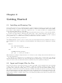
Chapter 2
Getting Started
2.1
Installing and Running Clus
Clus is written in the Java programming language, which is available from http://java.sun.com. You will
need Java version 1.5.x or newer. To run Clus, it suffices to install the Java Runtime Environment (JRE).
If you want to make changes to Clus and compile its source code, then you will need to install the Java
Development Kit (JDK) instead of the JRE.
The Clus software is released under the GNU General Public License version 3 or later and is available
for download at http://www.cs.kuleuven.be/~dtai/clus/. After downloading Clus, unpack it into a
directory of your choice. Clus is a command line application and should be started from the command
prompt (Windows) or a terminal window (Unix). To start Clus, enter the command:
java -jar $CLUS_DIR/Clus.jar filename.s
with $CLUS_DIR/Clus.jar the location of Clus.jar in your Clus distribution and filename.s the name of
your settings file. In order to verify that your Clus installation is working properly, you might try something
like:
Windows:
cd C:\Clus\data\weather
java -jar ..\..\Clus.jar weather.s
Unix:
cd $HOME/Clus/data/weather
java -jar ../../Clus.jar weather.s
This runs Clus on a simple example Weather. You can also try other example data sets in the data directory
of the Clus distribution.
Note that the above instructions are for running the pre-compiled version of Clus (Clus.jar), which is
included with the Clus download. If you have modified and recompiled Clus, or if you are using the SVN
developers version, then you should run Clus in a different way, as is explained in Chapter 7.
2.2
Input and Output Files for Clus
Clus uses (at least) two input files and these are named filename.s and filename.arff, with filename
a name chosen by the user. The file filename.s contains the parameter settings for Clus. The file
filename.arff contains the training data to be read. The format of the data file is Weka’s ARFF format1 .
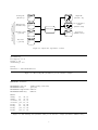
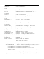
The results of a Clus run are put in an output file filename.out. Figure 2.1 gives an overview of the input
and output files supported by Clus. The format of the data files is described in detail in Chapter 3, the
format of the settings file is discussed in Chapter 4, and the output files are covered in Chapter 6. Optionally,
Clus can also generate a detailed output of the cross-validation (weather.xval) and model predictions in
ARFF format.
1 http://weka.wikispaces.com/ARFF
4
Input data in ARFF format
Settings file
(filename.s)
Output file
(filename.out)
[Model]
MinimalWeight = 2.0
[Tree]
FTest = 1.0
...
Training data
(filename.arff)
Cross-validation
details
(filename.xval)
@relation data
@attribute x 0,1
@attribute y numeric
@data
0,0.5
1,0.75
...
Clus system
Validation data
(optional)
@relation data
@attribute x 0,1
@attribute y numeric
@data
0,0.5
1,0.75
...
Test data
(optional)
@relation data
@attribute x 0,1
@attribute y numeric
@data
0,0.5
1,0.75
...
@relation data
@attribute x 0,1
@attribute y numeric
@data
0,0.5
1,0.75
...
Predictions
(ARFF format)
...
Figure 2.1: Input and output files of Clus.
[Attributes]
Descriptive = 1-2
Target = 3-4
Clustering = 3-4
[Tree]
Heuristic = VarianceReduction
Figure 2.2: The settings file (weather.s) for the Weather example.
@RELATION "weather"
@ATTRIBUTE
@ATTRIBUTE
@ATTRIBUTE
@ATTRIBUTE
outlook
windy
temperature
humidity
@DATA
sunny,
sunny,
overcast,
overcast,
rainy,
rainy,
rainy,
rainy,
34,
30,
20,
11,
20,
18,
10,
8,
no,
no,
no,
yes,
no,
no,
yes,
yes,
{sunny,rainy,overcast}
{yes,no}
numeric
numeric
50
55
70
75
88
95
95
90
Figure 2.3: The training data (weather.arff) for the Weather example (in Weka’s ARFF format).
5
2.3
A Step-by-step Example
The Clus distribution includes a number of example datasets. In this section we briefly take a look at the
Weather dataset, and how it can be processed by Clus. We use Unix notation for paths to filenames; in
Windows notation the slashes become backslashes (see also previous section).
1. Move to the directory Clus/data/weather, which contains the Weather dataset:
cd Clus/data/weather
2. First inspect the file weather.arff. Its contents is also shown in Figure 2.3. This file contains the
input data that Clus will learn from. It is in the ARFF format: first, the name of the table is given;
then, the attributes and their domains are listed; finally, the table itself is listed.
3. Next, inspect the file weather.s. This file is also shown in Figure 2.2. It is the settings file, the file
where Clus will find information about the task it should perform, values for its parameters, and other
information that guides it behavior.
The Weather example is a small multi-target or multi-task learning problem [9], in which the goal
is to predict the target attributes temperature and humidity from the input attributes outlook and
windy. This kind of information is what goes in the settings file. The parameters under the heading
[Attributes] specify the role of the different attributes. In our learning problem, the first two
attributes (attributes 1-2: outlook and windy) are descriptive attributes: they are to be used in the
cluster descriptions, that is, in the tests that appear in the predictive clustering tree’s nodes (or, in rule
learning, the conditions that appear in predictive clustering rules). The last two attributes (attributes
3-4) are so-called target attributes: these are to be predicted from the descriptive attributes. The setting
Clustering = 3-4 indicates that the clustering heuristic, which is used to construct the tree, should
be computed based on the target attributes only. (That is, Clus should try to produce clusters that are
coherent with respect to the target attributes, not necessarily with respect to all attributes.) Finally, in
the Tree section of the settings file, which contains parameters specific to tree learning, Heuristic =
VarianceReduction specifies that, among different clustering heuristics that are available, the heuristic
that should be used for this run is variance reduction.
These are only a few possible settings. Chapter 4 provides a detailed description of each setting
supported by Clus.
4. Now that we have some idea of what the settings file and data file look like, let’s run Clus on these
data and see what the result is. From the Unix command line, type, in the directory where the weather
files are:
java -jar ../../Clus.jar weather.s
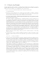
5. Clus now reads the data and settings files, performs it computations, and writes the resulting predictive
clustering tree, together with a number of statistics such as the training set error and the test set error
(if a test set has been provided), to an output file, weather.out. Open that file and inspect its
contents; it should look like the file shown in Figure 2.4. The file contains information about the Clus
run, including some statistics, and of course also the final result: the predictive clustering tree that we
wanted to learn. By default, Clus shows both an “original model” (the tree before pruning it) and a
“pruned model”, which is a simplified version of the original one.
In this example, the resulting tree is a multi-target tree: each leaf predicts a vector of which the first
component is the predicted temperature (attribute 3) and the second component the predicted humidity
(attribute 4). A feature that distinguishes Clus from other decision tree learners is exactly the fact
that Clus can produce this kind of trees. Constructing a multi-target tree has several advantages
over constructing a separate regression tree for each target variable. The most obvious one is the
number of models: the user only has to interpret one tree instead of one tree for each target. A second
advantage is that the tree makes features that are relevant to all target variables explicit. For example,
the first leaf of the tree in Figure 2.4 shows that outlook = sunny implies both a high temperature
and a low humidity. Finally, due to so-called inductive transfer, multi-target PCTs may also be more
accurate than regression trees. More information about multi-target trees can be found in the following
publications: [5, 4, 24, 19].
6
Clus run "weather"
******************
Date: 1/10/10 12:23 PM
File: weather.out
Attributes: 4 (input: 2, output: 2)
[Data]
File = weather.arff
[Attributes]
Target = 3-4
Clustering = 3-4
Descriptive = 1-2
[Tree]
Heuristic = VarianceReduction
PruningMethod = M5
Statistics
---------Induction Time: 0.017 sec
Pruning Time: 0.001 sec
Model information
Original: Nodes = 7 (Leaves: 4)
Pruned: Nodes = 3 (Leaves: 2)
Training error
-------------Number of examples: 8
Mean absolute error (MAE)
Default
: [7.125,14.75]: 10.9375
Original
: [2.125,2.75]: 2.4375
Pruned
: [4.125,7.125]: 5.625
Mean squared error (MSE)
Default
: [76.8594,275.4375]: 176.1484
Original
: [6.5625,7.75]: 7.1562
Pruned
: [19.4375,71.25]: 45.3438
Original Model
**************
outlook = sunny
+--yes: [32,52.5]: 2
+--no: outlook = rainy
+--yes: windy = yes
|
+--yes: [9,92.5]: 2
|
+--no: [19,91.5]: 2
+--no: [15.5,72.5]: 2
Pruned Model
************
outlook = sunny
+--yes: [32,52.5]: 2
+--no: [14.5,85.5]: 6
Figure 2.4: The Weather example’s output (weather.out). (Some parts have been omitted for brevity.)
7
Chapter 3
Input Format
Like many machine learning systems, Clus learns from tabular data. These data are assumed to be in the
ARFF format that is also used by the Weka data mining tool. Full details on ARFF can be found elsewhere1 .
We only give a minimal description here.
In the data table, each row represents an instance, and each column represents an attribute of the
instances. Each attribute has a name and a domain (the domain is the set of values it can take). In the
ARFF format, the names and domains of the attributes are declared up front, before the data are given.
The syntax is not case sensitive. An ARFF file has the following format:
% all comment lines are optional, start with %, and can occur
% anywhere in the file
@RELATION name
@ATTRIBUTE name domain
@ATTRIBUTE name domain
...
@DATA
value1 , value2 , ... , valuen
value1 , value2 , ... , valuen
The domain of an attribute can be one of:
• numeric
• { nomvalue1 , nomvalue2 , ... , nomvaluen }
• string
• hierarchical hvalue1 , hvalue2 , ... , hvaluen
• timeseries
The first option, numeric (real and integer are also legal and are treated in the same way), indicates that
the domain is the set of real numbers. The second type of domain is called a discrete domain. Discrete
domains are defined by enumerating the values they contain. These values are nominal. The third domain
type is string and can be used for attributes containing arbitrary textual values.
The fourth type of domain is called hierarchical (multi-label). It implies two things: first, the attribute
can take as a value a set of values from the domain, rather than just a single value; second, the domain has a
hierarchical structure. The elements of the domain are typically denoted v1 /v2 /.../vi , with i ≤ d, where d is
the depth of the hierarchy. A set of such elements is denoted by just listing them, separated by @. This type
of domain is useful in the context of hierarchical multi-label classification and is not part of the standard
ARFF syntax.
1 http://weka.wikispaces.com/ARFF
8
@RELATION HMCNewsGroups
@ATTRIBUTE word1
{1,0}
...
@ATTRIBUTE word100 {1,0}
@ATTRIBUTE class hierarchical rec/sport/swim,rec/sport/run,rec/auto,alt/atheism,...
@DATA
1,...,1,rec/sport/swim
1,...,1,rec/sport/run
1,...,1,rec/sport/run@rec/sport/swim
1,...,0,rec/sport
1,...,0,rec/auto
0,...,0,alt/atheism
...
Figure 3.1: An ARFF file that includes a hierarchical multi-label attribute.
@RELATION GeneExpressionTimeSeries
@ATTRIBUTE
@ATTRIBUTE
@ATTRIBUTE
...
@ATTRIBUTE
@ATTRIBUTE
@ATTRIBUTE
geneid string
GO0000003 {1,0}
GO0000004 {1,0}
GO0051704 {1,0}
GO0051726 {1,0}
target timeseries
@DATA
YAL001C,0,0,0,0,0,0,0,0,0,0,0,0,0,...,0,0,0,0,[0.07,
YAL002W,0,0,0,0,0,0,0,0,0,0,1,0,0,...,1,1,0,0,[0.14,
YAL003W,0,0,0,0,0,0,0,0,0,0,0,0,0,...,0,0,0,0,[0.46,
YAL005C,0,0,0,0,0,0,0,0,0,0,0,0,0,...,1,1,0,0,[0.86,
YAL007C,0,0,0,0,0,0,0,0,0,0,0,0,0,...,1,1,0,0,[0.12,
YAL008W,0,1,0,0,0,0,0,0,0,0,0,0,0,...,0,0,0,0,[0.49,
...
0.15,
0.14,
0.33,
1.19,
0.49,
1.01,
0.14, 0.15,-0.11, 0.07,-0.41]
0.18, 0.14, 0.17, 0.13, 0.07]
0.04,-0.60,-0.64,-0.51,-0.36]
1.58, 0.93, 1,
0.85, 1.24]
0.62, 0.49, 0.84, 0.89, 1.08]
1.33, 1.23, 1.32, 1.03, 1.14]
Figure 3.2: An ARFF file that includes a time series attribute.
The last type of domain is timeseries. A time series is a fixed length series of numeric data where
individual numbers are written in brackets and separated with commas. All time series of a given attribute
must be of the same length. This domain type, too, is not part of the standard ARFF syntax.
The values in a row occur in the same order as the attributes: the i’th value is assigned to the i’th
attribute. The values must, obviously, be elements of the specified domain.
Clus also supports the sparse ARFF format, where only non-zero data values are stored for the numeric
attributes. The header of a sparse ARFF file is the same, but each data instance is written in curly braces
and each attribute value is written as a pair of the attribute number (starting from one) and its value
separated by a space; values of different attributes are separated by commas.
Figure 2.3 shows an example of an ARFF file. An example of a table containing hierarchical multi-label
attributes is shown in Figure 3.1, an example ARFF file with a time series attribute is shown in Figure 3.2,
and an example sparse ARFF file is shown in Figure 3.3.
9
@RELATION SparseData
@ATTRIBUTE
@ATTRIBUTE
...
@ATTRIBUTE
@ATTRIBUTE
@ATTRIBUTE
@DATA
{1 3.1,
{7 2.3,
{2 8.5,
{1 3.2,
{1 3.3,
...
a1
a2
numeric
numeric
a10
numeric
a11
numeric
class {pos,neg}
8 2.5, 12 pos}
12 neg}
3 1.3, 12 neg}
12 pos}
8 2.7, 12 pos}
Figure 3.3: An ARFF file in sparse format.
10
Chapter 4
Settings File
The algorithms included in the Clus system have a number of parameters that influence their behavior.
Most parameters have a default setting; the specification of a value for such parameters is optional. For
parameters that do not have a default setting or which should get another value than the default, a value
must be specified in the settings file, filename.s.
The settings file is structured into sections. Each parameter belongs to a particular section. Including
the section headers (section names written in brackets) is optional, however; these headers are meant to help
users structure the settings and their use is recommended.
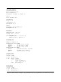
We here explain the most common settings. Some settings that are connected to experimental or not yet
fully implemented features of Clus are either marked as such or not presented at all. Figure 4.1 shows an
example of a settings file. All the settings (including the default ones) that were used in a specific Clus run
are printed at the beginning of the output file (filename.out).
In the following, we use the convention that n is an integer, r is a real, v is a vector of real values, s is a
string, y is an element of { Yes, No }, r is an range of attribute indices, and o is another type of value. Strings
are denoted without quotes. A vector is denoted as [r1 , . . . , rn ]. An attribute range is a comma separated
list of integers or intervals or None if the range is empty. For example, 5,7-9 indicates attributes 5, 7, 8
and 9. The first attribute in the dataset is attribute 1. Run clus -info filename.s to list all attributes
together with their indices. We now explain the settings organized into sections.
4.1
General
• RandomSeed = n : n is used to initialize the random generator. Some procedures used by Clus (e.g.,
creation of cross-validation folds) are randomized, and as a result, different runs of Clus on identical
data may still yield different outputs. When Clus is run on identical input data with the same
RandomSeed setting, it is guaranteed to yield the same results.
4.2
Data
• File = s : s is the name of the file that contains the training set. The default value for s is
filename.arff. Clus can read compressed (.arff.zip) or uncompressed (.arff) data files. Path
can also be included in the string.
• TestSet = o : when o is None, no test set is used; if o is a number between 0 and 1, Clus will use a
proportion o of the data file as a separate test set (used for evaluating the model but not for training);
if o is a valid file name containing a test set in ARFF format, Clus will evaluate the learned model
on this test set.
• PruneSet = o : defines whether and how to use a pruning set; the meaning of o is identical as in the
TestSet setting.
• XVal = n : n is the number of folds to be used in a cross-validation. To perform cross-validation,
Clus needs to be run with the -xval command line parameter.
11
4.3
Attributes
• Target = r : sets the range of target attributes. The predictive clustering model will predict these
attributes. If this setting is not specified, then it is equal to the index of the last attribute in the
training dataset, i.e., the last attribute is the target by default. This setting overrides the Disable
setting. This is convenient if one needs to build models that predict only a subset S of all available
target attributes T (and other target attributes should not be used as descriptive attributes). Because
Target overrides Disable, one can use the settings Disable = T and Target = S to achieve this.
• Clustering = r : sets the range of clustering attributes. The predictive clustering heuristic that is
used to guide the model construction is computed with regard to these atrributes. If this setting is not
specified, then the clustering attributes are by default equal to the target attributes.
• Descriptive = r : sets the range of attributes that can be used in the descriptive part of the models.
For a PCT, these attributes will be used to construct the tests in the internal nodes of the tree. For
a set of PCRs, these attributes will appear in the rule conditions. If this setting is not specified, then
the descriptive attributes are all attributes that are not target, key, or disabled.
• Disable = r : sets the range of attributes that are to be ignored by Clus. These attributes are also
not read into memory.
• Key = r : sets the range of key attributes. A key attribute or a set of key attributes can be used as
an example identifier. For example, if each instance represents a person, then the key attribute could
store the person’s name. Key attributes are not actually used by the induction algorithm, but they are
written to output files, for example, to ARFF files with predictions. See [Output]/WritePredictions
for an example.
• Weights = o : sets the relative weights of the different attributes in the clustering heuristic. To set
the weights of all clustering attributes to 1.0, use Weights = 1. To use as weights wi = 1/Var(ai ),
with Var(ai ) the variance of attribute ai in the input data, use Weights = Normalize.
4.4
Model
• MinimalWeight = r : Clus only generates clusters with at least r instances in each subset (tree leaves
or rules). This is a standard setting used for pre-pruning of trees and rules.
4.5
Tree
• FTest = r : sets the f-test stopping criterion for regression; a node will only be split if a statistical Ftest indicates a significant (at level r) reduction of variance inside the subsets. The f-test level can also
be optimized by providing a vector of levels, e.g. FTest = [0.001,0.005,0.01,0.05,0.1,0.125]. In
that case, the (smallest) f-test level will be chosen that minimizes the RMSE measure on the validation
set provided (using the PruneSet setting).
• ConvertToRules = o : o is an element of {No, Leaves, AllNodes}. Clus can convert a tree (or
ensemble of trees) into a set of rules. The default setting is No, if set to Leaves, only tree leaves are
converted to rules, if set to AllNodes, also the internal nodes of tree(s) are converted. This setting
can be used for learning rule ensembles [1].
• SplitSampling = s : the split heuristic can be calculated on a sample of the training set. For s > 0,
the training set is, for each split, sampled with replacement to form a sample of size s. The default
setting is s = None, the training set is used as is.
• Heuristic = o : o is an element of {Default, ReducedError, Gain, GainRatio,
VarianceReduction, MEstimate, Morishita, DispersionAdt, DispersionMlt,
RDispersionAdt, RDispersionMlt}. Sets the heuristic function that is used for evaluating the
clusters (splits) when generating trees or rules. Please note that this setting is used for trees as well
as rules.
– Default: default heuristic, if learning trees this is equal to VarianceReduction, if learning rules
this setting is equal to RDispersionMlt.
12
– ReducedError: reduced error heuristic, can be used for trees.
– Gain: information gain heuristic, can be used for classification trees.
– GainRatio: information gain ratio heuristic [20], can be used for classification trees.
– VarianceReduction: variance reduction heuristic, can be used for trees.
– MEstimate: m-estimate heuristic [10], can be used for classification trees.
– Morishita: Morishita heuristic [23], can be used for trees.
– DispersionAdt: additive dispersion heuristic [27] pages 37–38, can be used for rules.
– DispersionMlt: multiplicative dispersion heuristic [27] pages 37–38, can be used for rules.
– RDispersionAdt: additive relative dispersion heuristic [27] pages 37–38, can be used for rules.
– RDispersionMlt: multiplicative relative dispersion heuristic [27] pages 37–38, can be used for
rules, the default heuristic for learning predictive clustering rules.
• PruningMethod = o : o is an element of {Default, None, C4.5, M5, M5Multi,
ReducedErrorVSB, Garofalakis, GarofalakisVSB, CartVSB, CartMaxSize}. Sets the
post-pruning method for trees.
– Default: default pruning method for trees, if learning classification trees this is equal to C4.5, if
learning regression trees this is equal to M5.
– None: no post-pruning of learned trees is performed.
– C4.5: pruning as in C4.5 [22], can be used for classification trees,
– M5: pruning as in M5 [21], can be used for regression trees,
– M5Multi: experimental modification to M5 [21] pruning for multi-target regression trees.
– ReducedErrorVSB: reduced error pruning where the error is estimated on a separate validation
data set (VSB = validation set based pruning).
– Garofalakis: pruning method proposed by Garofalakis et al. [13] used for constraint induction
of trees.
– GarofalakisVSB: same as Garofalakis, but the error is estimated on a separate validation data
set.
– CartVSB: pruning method that is implemented in CART [8], and uses a separate validation set.
It seems to work better than M5 on the multi-target regression data sets.
– CartMaxSize: pruning method that is also implemented in CART [8], but uses cross-validation
to tune the pruning parameter to achieve the desired tree size.
4.6
Rules
• Heuristic = o : determines the heuristic for rule learning; see the Tree section for details.
• CoveringMethod = o : o is an element of {Standard, WeightedError, RandomRuleSet, HeurOnly,
RulesFromTree}. Defines how the rules are generated.
– Standard: standard covering algorithm [17], all examples covered by the new rule are removed
from the current learning set, can be used for learning ordered rules.
– WeightedError: error weighted covering algorithm [27] (Section 4.5), examples covered by the
new rule are not removed from the current learning set, but their weight is decreased inversely
proportional to the error the new rule makes when predicting their target values, can be used for
learning unordered rules.
– RandomRuleSet: rules are generated randomly, (experimental feature).
– HeurOnly: no covering is used, the heuristic function takes into account the already learned rules
and the examples they cover to focus on yet uncovered examples, (experimental feature).
– RulesFromTree: rules are not learned with the covering approach, but a tree is learned first and
then transcribed into a rule set. After this e.g. rule weight optimization methods can be used.
13
• CoveringWeight = r : weight controlling the amount by which weights of covered examples are reduced within the error weighted covering algorithm – ζ in [27] (Section 4.5, Equations 4.6 and 4.8),
valid values are between 0 and 1, by default it is set to 0.1, can be used for unordered rules with error
weighted covering method.
• InstCoveringWeightThreshold = r : instance weight threshold used in error weighted covering algorithm for learning unordered rules. When an instance’s weight falls below this threshold, it is removed
from the current learning set. in [27] (Section 4.5), valid values are between 0 and 1, by default it is
set to 0.1.
• MaxRulesNb = n: n defines a maximum number of rules in a rule set. By default it is set to 1000.
• RuleAddingMethod = o : o is an element of {Always, IfBetter, IfBetterBeam}. Defines how rules
are added to the rule set.
– Always: each rule when constructed is always added to the rule set,
– IfBetter: rule is only added to the rule set if the performance of the rule set with the new rule
is better than without it,
– IfBetterBeam: similar to IfBetter, but if the rule does not improve the performance of the rule
set, other rules from the beam are also evaluated and possibly added to the rule set.
The default value is Always, for regression rules setting this option to IfBetter is recommended.
• PrintRuleWiseErrors = y: If Yes, Clus will print error estimation for each rule separately.
• ComputeDispersion = y: If Yes, Clus will print some additional dispersion estimation for each rule
and entire rule set.
• OptGDMaxIter = n : n defines a number of iterations that a gradient descent algorithm for optimizing
rule weights makes, used for learning rule ensembles [1]. The default value is 1000.
• OptGDMaxNbWeights = n: n defines a maximum number of of allowed nonzero weights for rules/linear
terms, used for learning rule ensembles [1]. If we have enough modified weights, only the nonzero ones
are altered for the rest of the optimization. With this we can limit the size of the rule set. The default
value of 0 means no rule set size limitation.
• OptGDGradTreshold = r : the τ treshold value for the gradient descent (GD) algorithm used for
learning rule ensembles [1]. τ defines the limit by which gradients are changed during every iteration
of the GD algorithm. If τ =1 effect is similar to L1 regularization (Lasso) and τ =0 the effect is similar
to L2. If OptGDMaxNbWeights is low (less than 40), setting τ =1 is usually enough (it is the fastest).
Possible values are from the [0,1] interval, the default is 1.
• OptGDNbOfTParameterTry = n : n defines how many different τ values are checked between 1 and
OptGDGradTreshold. We use a validation set to compute, which τ value gives the best accuracy. If
OptGDMaxNbWeights is low, usually only a single value τ =1 is enough (fastest). Default 1.
• OptGDEarlyTTryStop = y : When trying different τ values starting from 1, do we stop if validation
error starts to increase too much? Usually a lot faster, but may decrease the accuracy. Default Yes.
• OptGDStepSize = r : If OptGDIsDynStepsize is No, the initial gradient descent step size factor.
Default 0.1.
• OptGDIsDynStepsize = y : Do we use as the step size factor a lower limit of optimal one? The value
is computed based on the rule prediction values. Usually faster (lower step sizes are not tried at all)
and often also more accurate than a given value. Default Yes.
• OptAddLinearTerms = o : o is an element of {No, Yes, YesSaveMemory}. Defines whether to add
descriptive attributes as linear terms to the rule set. Usually this increases the accuracy. Especially for
multi-target data sets it also slows the algorithm down. For these, use value YesSaveMemory, otherwise
it can take a lot of memory. For single target data sets Yes is faster. Used for learning rule ensembles
[1].
14
• OptLinearTermsTruncate = y : Used in conjunction with the above OptAddLinearTerms setting. If
Yes, the linear terms are truncated so that they do not predict values greater or smaller than found
in the training set. This adds more robustness against outliers. The default setting is Yes. Used for
learning rule ensembles [1].
• OptNormalizeLinearTerms = o : o is an element of {No, Yes, YesAndConvert}. Defines whether
the linear terms are scaled so that each descriptive attribute has a similar effect. The default setting
is Yes and it should always be used. However, if you want to transform the rule ensemble so that
linear terms are of ”standard type”, you may use YesAndConvert setting. This moves the effect of
normalizations to weights and default prediction after optimization. Used for learning rule ensembles
[1].
4.7
Ensemble
• Iterations = n : n defines the number of base-level models (trees) in the ensemble, by default it is
set to 10.
• EnsembleMethod = o : o is an element of {Bagging, RForest, RSubspaces, BagSubspaces} defines
the ensemble method.
– Bagging: Bagging [6].
– RForest: Random forest [7].
– RSubspaces: Random Subspaces [14].
– BagSubspaces: Bagging of subspaces [18].
• BagSize = n: When using a bagging scheme in large datasets, it might be useful to control the size
of the individual bags. For n > 0, bags will have size n rather than size N (the size of the dataset).
• VotingType = o : o is an element of {Majority, ProbabilityDistribution} selects the voting
scheme for combining predictions of base-level models.
– Majority: each base-level model casts one vote, for regression this is equal to averageing.
– ProbabilityDistribution: each base-level model casts probability distributions for each target
attribute, does not work for regression.
The default value is Majority, Bauer and Kohavi [3] recommend ProbabilityDistribution.
• SelectRandomSubspaces = n : n defines size of feature subset for random forests, random subspaces
and bagging of subspaces. Default setting is 0, which means floor(log2 (number of descriptive attributes+
1)) as recommended by Breiman [7].
• PrintAllModels = y : If Yes, Clus will print all base-level models of an ensemble in the output file.
The default setting is No.
• PrintAllModelFiles = y: If Yes, Clus will save all base-level models of an ensemble in the model
file. The default setting is No, which prevents from creating very large model files.
• Optimize = y : If Yes, Clus will optimize memory usage during learning. The default setting is No.
• OOBestimate = y : If Yes, out-of-bag estimate of the performance of the ensemble will be done. The
default setting is No.
• FeatureRanking = y : If Yes, feature ranking via random forests will be performed. The default
setting is No.
• EnsembleRandomDepth = y : If Yes, different random depth for each base-level model is selected.
Used, e.g., in rule ensembles. The MaxDepth setting from [Tree] section is used as average. The
default setting is No.
15
4.8
Constraints
• Syntactic = o : sets the file with syntactic constraints (e.g., a partial tree) [24].
• MaxSize = o : sets the maximum size for Garofalakis pruning [13, 24]; o can be a positive integer or
Infinity.
• MaxError = o : sets the maximum error for Garofalakis pruning; o is a positive real or Infinity.
• MaxDepth = o : o is a positive integer or Infinity. Clus will build trees with depth at most o. In
the context of rule ensemble learning [1], this sets the average maximum depth of trees that are then
converted into rules and a value of 3 seems to work fine.
4.9
Output
• AllFoldModels = y : if set to Yes, Clus will output the model built in each fold of a cross-validation.
• AllFoldErrors = y : if set to Yes, Clus will output the test set error (and other evaluation measures)
for each fold.
• TrainErrors = y : if set to Yes, Clus will output the training set error (and other evaluation measures).
• UnknownFrequency = y : if set to Yes, Clus will show in each node of the tree the proportion of
instances that had a missing value for the test in that node.
• BranchFrequency = y : if set to Yes, Clus will show in each node of the tree, for each possible
outcome of the test in that node, the proportion of instances that had that outcome.
• WritePredictions = o : o is a subset of {Train,Test}. If o includes “Train”, then the prediction for
each training instance will be written to an ARFF output file. The file is named filename.train.
i.pred.arff with i the iteration. In a single run, i = 1. In a 10 fold cross-validation, i will vary from
1 to 10. If o includes “Test”, then the predictions for each test instance will be written to disk. The
file is named filename.test.pred.arff.
4.10
Beam
• SizePenalty = o : sets the size penalty parameter used in the beam heuristic [15].
• BeamWidth = n : sets the width of the beam used in the beam search performed by Clus [15].
• MaxSize = o : sets the maximum size constraint [15]; o is a positive integer or Infinity.
4.11
Hierarchical
A number of settings are relevant only when using Clus for Hierarchical Multi-label Classification (HMC).
These go in the separate section “Hierarchical”. The most important ones are:
• Type = o : o is Tree or DAG, and indicates whether the class hierarchy is a tree or a directed acyclic
graph [26]
• WType = o : defines how parents’ class weights are aggregated in DAG-shaped hierarchies ([26], Section 4.1): possible values are ExpSumParentWeight, ExpAvgParentWeight, ExpMinParentWeight,
ExpMaxParentWeight, and NoWeight. These define the weight of a class to be w0 times the sum,
average, minimum or maximum of the parent’s weights, respectively, or to be 1.0 for all classes.
• WParam = r : sets the parameter w0 used in the formula for defining the class weights ([26], Section
4.1)
• HSeparator = o : o is the separator used in the notation of values of the hierarchical domain (typically
‘/’ or ‘.’)
16
[General]
RandomSeed = 0
% seed of random generator
[Data]
File = weather.arff
TestSet = None
PruneSet = None
XVal = 10
%
%
%
%
training data
data used for evaluation (file name / proportion)
data used for tree pruning (file name / proportion)
number of folds in cross-validation (clus -xval ...)
[Attributes]
Target = 5
Disable = 4
Key = None
Weights = Normalize
%
%
%
%
index of target attributes
Disables some attributes (e.g., "5,7-8")
Sets the index of the key attribute
Normalize numeric attributes
[Model]
MinimalWeight = 2.0
% at least 2 examples in each subtree
[Tree]
FTest = 1.0
ConvertToRules = No
% f-test stopping criterion for regression
% Convert the tree to a set of rules
[Constraints]
Syntactic = None
MaxSize = Infinity
MaxError = Infinity
MaxDepth = Infinity
%
%
%
%
file with syntactic constraints (a partial tree)
maximum size for Garofalakis pruning
maximum error for Garofalakis pruning
Stop building the tree at the given depth
[Output]
AllFoldModels = Yes
% Output model in each cross-validation fold
AllFoldErrors = No
% Output error measures for each fold
TrainErrors = Yes
% Output training error measures
UnknownFrequency = No
% proportion of missing values for each test
BranchFrequency = No
% proportion of instances for which test succeeds
WritePredictions = {Train,Test}
% write test set predictions to file
[Beam]
SizePenalty = 0.1
BeamWidth = 10
MaxSize = Infinity
% size penalty parameter used in the beam heuristic
% beam width
% Sets the maximum size constraint
Figure 4.1: An example settings file
• EmptySetIndicator = o : o is the symbol used to indicate the empty set
• OptimizeErrorMeasure = o : Clus can automatically optimize the FTest setting (see earlier); o
indicates what criterion should be maximized for this ([26], Section 5.2). Possible values for o are:
– AverageAUROC: average of the areas under the class-wise ROC curves
– AverageAUPRC: average of the areas under the class-wise precision-recall curves
– WeightedAverageAUPRC: similar to AverageAUPRC, but each class’s contribution is weighted by
its relative frequency
– PooledAUPRC: area under the average (or pooled) precision-recall curve
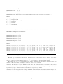
• ClassificationThreshold = o : The original tree constructed by Clus contains a vector of predicted
probabilities (one for each class) in each leaf. Such a probabilistic prediction can be converted into a
17
[Hierarchical]
Type = Tree
WType = ExpAvgParentWeight
WParam = 0.75
HSeparator = /
EmptySetIndicator = n
OptimizeErrorMeasure = PooledAUPRC
ClassificationThreshold = None
RecallValues = None
EvalClasses = None
MEstimate = No
%
%
%
%
%
%
%
%
%
%
Tree or DAG hierarchy?
aggregation of class weights
parameter w_0
separator used in class names
symbol for empty set
FTest optimization strategy
threshold for "positive"
where to report precision
classes to evaluate
whether to use m-estimate in the prediction vector
Figure 4.2: Settings specific for hierarchical multi-label classification
set of labels by applying a threshold t: all labels that are predicted with probability ≥ t are in the
predicted set. o can be a list of thresholds, e.g., [0.5, 0.75, 0.80, 0.90, 0.95]. Clus will output for each
value in the set a tree in which the predicted label sets are constructed with this particular threshold.
So, in the example, the output file will contain 5 trees corresponding to the thresholds 0.5, 0.75, 0.80,
0.90 and 0.95.
• RecallValues = v : v is a list of recall values, e.g., [0.1, 0.2, 0.3]. For each value, Clus will output
the average of the precisions over all class-wise precision-recall curves that correspond to the particular
recall value in the output file.
• EvalClasses = o : If o is None, Clus computes average error measures across all classes in the class
hierarchy. If o is a list of classes, then the error measures are only computed with regard to the classes
in this list.
• MEstimate = y : if set to Yes, Clus will apply an m-estimate in the prediction vector of each leaf.
For each leaf and each label, define T = total training examples and P = number of positive training
examples. With the m-estimate, instead of predicting P/T for the given label, we predict (P + p ∗
T 0 )/(T + T 0 ), i.e. we act as if we have seen T 0 extra (“virtual”) examples of which p are positive, where
T 0 and p are parameters. In the Clus implementation, T 0 = 1 and p is the proportion of positive
examples in the full training set. So the predictions in the leaf for a given label are interpreted as
(P + p)/(T + 1).
Figure 4.2 summarizes these settings briefly.
18
Chapter 5
Command Line Parameters
Clus is run from the command line. It takes a number of command line parameters that affect its behavior.
• -xval : in addition to learning a single model from the whole input dataset, perform a cross-validation.
The XVal setting (page 11) determines the number of folds; the RandomSeed setting (page 11) initializes the random generator that determines the folds.
• -fold N : run only fold N of the cross-validation.
• -rules : construct predictive clustering rules (PCRs) instead of predictive clustering trees (PCTs).
• -forest : construct an ensemble instead of a single tree [16].
• -beam : construct a tree using beam search [15].
• -sit : run Empirical Asymmetric Selective Transfer [19].
• -silent : run Clus with reduced screen output.
• -info : gives information and summary statistics about the dataset.
19
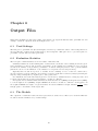
Chapter 6
Output Files
When Clus is finished, it writes the results of the run into an output file with the name filename.out. An
example of such an output file is shown in Figures 6.1 to 6.4.
6.1
Used Settings
The first part of filename.out (shown in Figures 6.1 and 6.2) contains the values of the settings that were
used for this run of Clus, in the format used by the settings file. This part can be copied and pasted to
filename.s and modified for subsequent runs.
6.2
Evaluation Statistics
The next part contains statistics about the results of this Clus run.
Summary statistics about the running time of Clus and about the size of the resulting models are given.
Next, information on the models’ predictive performance on the training set (“training set error”) is given,
as well as an estimate of its predictive performance on unseen examples (“test set error”), when available
(this is the case if a cross-validation or an evaluation on a separate test set was performed).
Typically three models are reported: a “default” model consisting of a tree of size zero, which can be
used as a reference point (for instance, its predictive accuracy equals that obtained by always predicting the
majority class); an unpruned (“original”) tree, and a pruned tree.
For classification trees the information given for each model by default includes a contingency table, and
(computed from that) the accuracy and Cramer’s correlation coefficient.
For regression trees, this information includes the mean absolute error (MAE), mean squared error (MSE),
root mean squared error (RMSE), weighted RMSE, the Pearson correlation coefficient r and it square. In
, with
the weighted RMSE, the weight of a given attribute A is its normalization weight, which is √ 1
Var(A)
Var(A) equal to A’s variance in the input data.
6.3
The Models
The output file contains the learned models, represented as decision trees. The level of detail in which the
models are shown is influenced by certain settings.
20
Clus run "weather"
******************
Date: 1/10/10 4:37 PM
File: weather.out
Attributes: 4 (input: 2, output: 2)
Missing values: No
[General]
Verbose = 1
Compatibility = Latest
RandomSeed = 0
ResourceInfoLoaded = No
[Data]
File = weather.arff
TestSet = None
PruneSet = None
XVal = 10
RemoveMissingTarget = No
NormalizeData = None
[Attributes]
Target = 3-4
Clustering = 3-4
Descriptive = 1-2
Key = None
Disable = None
Weights = Normalize
ClusteringWeights = 1.0
ReduceMemoryNominalAttrs = No
[Constraints]
Syntactic = None
MaxSize = Infinity
MaxError = 0.0
MaxDepth = Infinity
[Output]
ShowModels = {Default, Pruned, Others}
TrainErrors = Yes
ValidErrors = Yes
TestErrors = Yes
AllFoldModels = Yes
AllFoldErrors = No
AllFoldDatasets = No
UnknownFrequency = No
BranchFrequency = No
ShowInfo = {Count}
PrintModelAndExamples = No
WriteErrorFile = No
WritePredictions = {None}
WriteModelIDFiles = No
WriteCurves = No
OutputPythonModel = No
OutputDatabaseQueries = No
Figure 6.1: Example output file (part 1, settings).
21
[Nominal]
MEstimate = 1.0
[Model]
MinimalWeight = 2.0
MinimalNumberExamples = 0
MinimalKnownWeight = 0.0
ParamTuneNumberFolds = 10
ClassWeights = 0.0
NominalSubsetTests = Yes
[Tree]
Heuristic = VarianceReduction
PruningMethod = M5
M5PruningMult = 2.0
FTest = 1.0
BinarySplit = Yes
ConvertToRules = No
AlternativeSplits = No
Optimize = {}
MSENominal = No
Figure 6.2: Example output file (part 2, settings (ctd.)).
Run: 01
*******
Statistics
---------FTValue (FTest): 1.0
Induction Time: 0.018 sec
Pruning Time: 0.001 sec
Model information
Default: Nodes = 1 (Leaves: 1)
Original: Nodes = 7 (Leaves: 4)
Pruned: Nodes = 3 (Leaves: 2)
Training error
-------------Number of examples: 8
Mean absolute error (MAE)
Default
: [7.125,14.75]: 10.9375
Original
: [2.125,2.75]: 2.4375
Pruned
: [4.125,7.125]: 5.625
Mean squared error (MSE)
Default
: [76.8594,275.4375]: 176.1484
Original
: [6.5625,7.75]: 7.1562
Pruned
: [19.4375,71.25]: 45.3438
Root mean squared error (RMSE)
Default
: [8.7669,16.5963]: 13.2721
Original
: [2.5617,2.7839]: 2.6751
Pruned
: [4.4088,8.441]: 6.7338
Weighted root mean squared error (RMSE) (Weights [0.013,0.004])
Default
: [1,1]: 1
Original
: [0.2922,0.1677]: 0.2382
Pruned
: [0.5029,0.5086]: 0.5058
Pearson correlation coefficient
Default
: [?,?], Avg r^2: ?
Original
: [0.9564,0.9858], Avg r^2: 0.9432
Pruned
: [0.8644,0.861], Avg r^2: 0.7442
Figure 6.3: Example output file (part 3, statistics).
22
Default Model
*************
[18.875,77.25]: 8
Original Model
**************
outlook = sunny
+--yes: [32,52.5]: 2
+--no: outlook = rainy
+--yes: windy = yes
|
+--yes: [9,92.5]: 2
|
+--no: [19,91.5]: 2
+--no: [15.5,72.5]: 2
Pruned Model
************
outlook = sunny
+--yes: [32,52.5]: 2
+--no: [14.5,85.5]: 6
Figure 6.4: Example output file (part 4, learned models).
23
Chapter 7
Developer Documentation
7.1
Compiling Clus
Note: The Clus download comes with a pre-compiled version of Clus stored in the file Clus.jar. So, if you
just want to run Clus as it is on a data set, then you do not need to compile Clus. You can run it by
following the instructions in Section 2.1. On the other hand, if you wish to modify the source code of Clus,
or if you are using the SVN version, then you will need to compile the source code of Clus. This can be
done using the commands below or using the Eclipse IDE as pointed out in the next section.
The SVN developers’ version of Clus is available at http://sourceforge.net/projects/clus/.
(Windows)
cd C:\Clus\src
javac -d "bin" -cp ".;jars\commons-math-1.0.jar;jars\jgap.jar" clus/Clus.java
(Unix)
cd /home/john/Clus
javac -d "bin" -cp ".:jars/commons-math-1.0.jar:jars/jgap.jar" clus/Clus.java
This will compile Clus and write the resulting .class files (Java executable byte code) to the ”bin” subdirectory. Alternatively, use the ”./compile.sh” script provided in the Clus main directory.
7.2
Compiling Clus with Eclipse
In Eclipse, create a new project for Clus as follows:
• Choose File | New | Project.
• Select ”Java Project” in the dialog box.
• In the ”New Java Project” dialog box:
– Enter ”Clus” in the field ”Project Name”.
– Choose ”Create project from existing source” and browse to the location where you unzipped
Clus. E.g., /home/john/Clus or C:\Clus.
– Click ”Next”.
– Select the ”Source” tab of the build settings dialog box. Change ”Default output folder” (where
the class files are generated) to: ”Clus/bin”.
– Select the ”Libraries” tab of the build settings dialog box. Click ”Add external jars” and add in
this way these three jars:
Clus/jars/commons-math-1.0.jar
Clus/jars/jgap.jar
Clus/jars/weka.jar
24
– Click ”Finish”.
• Select the ”Navigator” view (Choose Window — Show View — Navigator)
– Right click the ”Clus” project in this view.
– Select ”Properties” from the context menu.
– Select the ”Java Compiler” tab.
– Set the ”Java Compliance Level” to 5.0.
Now Clus should be automatically compiled by Eclipse. To run Clus from Eclipse:
• Set as main class ”clus.Clus”.
• Set as arguments the name of your settings file (appfile.s).
• Set as working directory, the directory on the file system where your data set is located.
7.3
Running Clus after Compiling the Source Code
These instructions are for running Clus after you compiled its source code (using the instructions ”Compiling
Clus” or ”Compiling Clus with Eclipse”). To run the pre-compiled version that is available in the file
”Clus.jar”, see Section 2.1.
(Windows)
cd path\to\appfile.s
java -cp "C:\Clus\bin;C:\Clus\jars\commons-math-1.0.jar;C:\Clus\jars\jgap.jar"
clus.Clus appfile.s
(Unix)
cd path/to/appfile.s
java -cp "$HOME/Clus/bin:$HOME/Clus/jars/commons-math-1.0.jar:$HOME/Clus/jars/jgap.jar"
clus.Clus appfile.s
Alternatively, use the ”./clus.sh” script provided in the Clus main directory after adjusting the line that
defines CLUS DIR at the top of the script.
7.4
Code Organization
Here we only provide a rough guide to the Clus code by listing some of the key classes and packages.
clus/Clus.java the main class with the main method, which is called when starting Clus.
clus/algo package with learning algorithms, e.g., sub-package clus/algo/tdidt includes tree learning
algorithm and clus/algo/rules includes rule learning algorithm, clus/algo/split includes classes
used for generating conditions in both trees and rules.
clus/data package with sub-packages and classes related to reading and storing of the data.
clus/error package where different error estimation measures are defined.
clus/ext some extensions of base tree learning methods can be found here, e.g., sub-package hierarchical
contains extensions needed for hierarchical classification, ensembles contains ensembles of trees and
timeseries contains extensions for predicting time-series data.
clus/heuristic contains classes implementing heuristic functions for tree learning (heuristics for rule learning are located in package clus/algo/rules).
clus/main contains some important support classes such as:
ClusRun.java
25
ClusStat.java
ClusStatManager.java
Settings.java all the Clus settings are defined here.
clus/model classes used for representations of models can be found here, including tests that appear in
trees and rules (clus/model/test).
clus/pruning contains methods for tree pruning.
clus/statistic contains classes used for storing and manipulating different information and statistics on
data. The key classes are:
ClusStatistic.java super class for all statistics used in Clus.
ClassificationStat.java class for storing information on nominal attributes (e.g., counts for each
possible nominal value)
RegressionStat.java class for storing information on numeric attributes (e.g., sums of values and
sums of squared values).
CombStat.java class for storing information on nominal and numeric attributes (contains ClassificationStat
and RegressionStat classes).
clus/tools contains some support code, e.g., sub-package optimization contains optimization procedures
used in rule ensemble learning.
clus/weka contains classes for interfacing with Weka machine learning package.
26
Acknowledgments
The research involved in development of this software was supported by the Research Foundation Flanders
(FWO-Vlaanderen) and the Slovenian Research Agency. We thank all our collaborators who have contributed
to the development of Clus, and in particular (in inverse alphabetical order) L. Schietgat, I. Slavkov, D.
Kocev, V. Gjorgjioski, E. Fromont and T. Aho.
27
Appendix A
Constructing Phylogenetic Trees
Using Clus
In this appendix, we describe the use of Clus-ϕ, a method for phylogenetic tree reconstruction [25]. Example
files can be found in the following directory:
$CLUS_DIR/data/phylo/.
The input to Clus-ϕ consists of a multiple alignment (in ARFF format), a settings file, and optionally
a distance matrix.
A.1
Input Format
Each position in the multiple alignment becomes an attribute in the ARFF file. The domain of these
attributes is discrete and will typically consist of the values A, C, T , and G for DNA sequences, and the
amino acids for protein sequences. If gaps occur, they have to be listed in the attribute domain. Gaps are
represented as ‘-’. Moreover, Clus-ϕ requires a string attribute, that contains an identifier for the sequence.
Perl scripts for converting PHY and FASTA files into the ARFF file format are available in the data/phylo/
directory.
A.2
Settings File
In order to construct phylogenetic trees, the settings file looks like the one shown in Fig. A.1. Apart from the
settings shown in the figure, there are a number of extra settings, specific for phylogenetic tree reconstruction
(see Fig. A.2). We discuss them in detail.
• Sequence = o : defines which type of sequences is used. Possible values for o are DNA, Protein, or
Any. The latter can be used in case a different alphabet than nucleotides or amino acids is used. The
default value for o is DNA.
• OptimizationCriterion = o : defines which criterion is optimized in the phylogenetic tree heuristic.
Possible values for o are MinTotBranchLength, for minimizing the total branch length of the tree,
and MaxAvgPWDistance, for maximizing the average pairwise distance between two subclusters (i.e.,
as done in the PTDC algorithm [2]). The default value for o is MinTotBranchLength.
• DistanceMatrix = s : s is the name of the optional pairwise distance matrix file. This file has to
be formatted in the same way as in the Phylip software package [12], i.e., the first line contains the
number of sequences, and then for each sequence there is a line starting with its identifier and listing
the pairwise distances to all the other sequences. See the example in the file mydistancematrix. The
rows in the distance matrix need to have the same ordering as the rows in the ARFF file.
• DistanceMeasure = o : defines which genetic distance is used between pairs of sequences, in the case
no distance matrix is given. Possible values for o are Edit for edit distance, PDist for p-distance, i.e.,
the same as edit distance, with positions with gaps or missing values discarded, JC for Jukes-Cantor
distance, Kimura for Kimura distance, and AminoKimura for Kimura distance between amino acid
sequences. See the Phylip documentation [12] for details.
28
[Tree]
PruningMethod = None
FTest = 1.0
AlternativeSplits = true
% Gives a listing of all equivalent mutations in the nodes
Heuristic = GeneticDistance
[Attributes]
Key = 1
Descriptive = 2-897
Target = 2-897
Weights = 1
% The identifier attribute
% All attributes corresponding to the alignment
% All attributes corresponding to the alignment
[Model]
MinimalWeight = 1
[Data]
File = chimp.arff
[Output]
TrainErrors = No
PrintModelAndExamples = true
Figure A.1: Required settings for learning phylogenetic trees
[Phylogeny]
Sequence = DNA
OptimizationCriterion = MinTotBranchLength
DistanceMatrix = mydistancematrix
DistanceMeasure = JC
Figure A.2: Optional settings for learning phylogenetic trees
A.3
Output Files
The filename.out file returned by Clus-ϕ can be postprocessed by the postprocess tree.pl perl script in
the data/phylo/ directory. This script returns two files: filename.clus-phy tree, which contains two tree
representations (one with just the topology, and one with all mutations listed), and filename.clus-phy newick,
which contains the tree in the so-called Newick format, where clusters are represented by pairs of parentheses.
29
Bibliography
[1] Timo Aho, Bernard Ženko, and Sašo Džeroski. Rule ensembles for multi-target regression. In Wei
Wang, Hillol Kargupta, Sanjay Ranka, Philip S. Yu, and Xindong Wu, editors, Proceedings of Ninth
IEEE International Conference on Data Mining (ICDM 2009), December 6-9, 2009, Miami Beach,
Florida, USA, pages 21–30. IEEE Computer Society, 2009.
[2] A. N. Arslan and P. Bizargity. Phylogeny by top down clustering using a given multiple alignment. In
Proceedings of the 7th IEEE Symposium on Bioinformatics and Biotechnology (BIBE 2007), Vol. II,
pages 809–814, 2007.
[3] Eric Bauer and Ron Kohavi. An empirical comparison of voting classification algorithms: Bagging,
boosting, and variants. Machine Learning, 36(1-2):105–139, 1999.
[4] H. Blockeel, S. Džeroski, and J. Grbović. Simultaneous prediction of multiple chemical parameters of
river water quality with Tilde. In Proceedings of the 3rd European Conference on Principles of Data
Mining and Knowledge Discovery, volume 1704 of Lecture Notes in Artificial Intelligence, pages 32–40.
Springer, 1999.
[5] H. Blockeel, L. De Raedt, and J. Ramon. Top-down induction of clustering trees. In Proceedings of the
15th International Conference on Machine Learning, pages 55–63, 1998.
[6] Leo Breiman. Bagging predictors. Machine Learning, 24(2):123–140, 1996.
[7] Leo Breiman. Random forests. Machine Learning, 45(1):5–32, 2001.
[8] Leo Breiman, Jerome H. Friedman, Richard A. Olshen, and Charles J. Stone. Classification and Regression Trees. Wadsworth International Group, Belmont, CA, USA, 1984.
[9] R. Caruana. Multitask learning. Machine Learning, 28:41–75, 1997.
[10] Bojan Cestnik. Estimating probabilities: A crucial task in machine learning. In L. Aiello, editor,
Proceedings of the Ninth European Conference on Artificial Intelligence (ECAI 90), pages 147–149,
London, UK/Boston, MA, USA, 1990. Pitman.
[11] P. Clark and R. Boswell. Rule induction with CN2: Some recent improvements. In Yves Kodratoff,
editor, Proceedings of the Fifth European Working Session on Learning, volume 482 of Lecture Notes in
Artificial Intelligence, pages 151–163. Springer-Verlag, 1991.
[12] J.
Felsenstein.
Phylip
(phylogeny
inference
http://evolution.genetics.washington.edu/phylip.html.
package)
version
3.68,
2008.
[13] M. Garofalakis, D. Hyun, R. Rastogi, and K. Shim. Building decision trees with constraints. Data
Mining and Knowledge Discovery, 7(2):187–214, 2003.
[14] Tin Kam Ho. The random subspace method for constructing decision forests. IEEE Transactions on
Pattern Analysis and Machine Intelligence, 20(8):832–844, 1998.
[15] D. Kocev, S. Džeroski, and J. Struyf. Beam search induction and similarity constraints for predictive
clustering trees. In 5th Int’l Workshop on Knowledge Discovery in Inductive Databases: Revised Selected
and Invited Papers, 2007. To appear.
[16] D. Kocev, C. Vens, J. Struyf, and S. Džeroski. Ensembles of multi-objective decision trees. In Proceedings
of the 18th European Conference on Machine Learning, pages 624–631. Springer, 2007.
30
[17] Ryszard S. Michalski. On the quasi-minimal solution of the general covering problem. In Proceedings
of the Fifth International Symposium on Information Processing (FCIP 69), volume A3, Switching
Circuits, pages 125–128, Bled, Yugoslavia, 1969.
[18] Panče Panov and Sašo Džeroski. Combining bagging and random subspaces to create better ensembles.
In Proceedings of Seventh International Symposium on Intelligent Data Analysis (IDA ’07), volume
4723 of Lecture Notes in Computer Science, pages 118–129, Berlin, Germany, 2007. Springer.
[19] B. Piccart, J. Struyf, and H. Blockeel. Empirical asymmetric selective transfer in multi-objective decision
trees. In Proceedings of the 11th International Conference on Discovery Science, volume 5255 of Lecture
Notes in Artificial Intelligence, pages 64–75, 2008.
[20] J. Ross Quinlan. Induction of decision trees. Machine Learning, 1(1):81–106, 1986.
[21] J. Ross Quinlan. Learning with continuous classes. In A. Adams and L. Sterling, editors, Proceedings
of the Fifth Australian Joint Conference on Artificial Intelligence, Hobart, Australia, November 16-18,
1992, pages 343–348, Singapore, 1992. World Scientific.
[22] J. Ross Quinlan. C4.5: Programs for Machine Learning. Morgan Kaufmann, San Francisco, CA, USA,
1993.
[23] Jun Sese and Shinichi Morishita. Itemset classified clustering. In Jean-François Boulicaut, Floriana
Esposito, Fosca Giannotti, and Dino Pedreschi, editors, Knowledge Discovery in Databases: PKDD
2004, Proceedings of the Eighth European Conference on Principles and Practice of Knowledge Discovery
in Databases, Pisa, Italy, September 20-24, 2004, Lecture Notes in Computer Science, pages 398–409,
Berlin, Germany, 2004. Springer.
[24] J. Struyf and S. Džeroski. Constraint based induction of multi-objective regression trees. In Knowledge
Discovery in Inductive Databases, 4th International Workshop, KDID’05, Revised, Selected and Invited
Papers, volume 3933 of Lecture Notes in Computer Science, pages 222–233, 2006.
[25] Celine Vens, Eduardo Costa, and Hendrik Blockeel. Top-down induction of phylogenetic trees. In
Proceedings of the 8th European Conference on Evolutionary Computation, Machine Learning and Data
Mining in Bioinformatics (EvoBIO 2010). Springer, 2010.
[26] Celine Vens, Jan Struyf, Leander Schietgat, Sašo Džeroski, and Hendrik Blockeel. Decision trees for
hierarchical multi-label classification. Machine Learning, 73(2):185–214, 2008.
[27] Bernard Ženko. Learning predictive clustering rules. PhD thesis, University of Ljubljana, Faculty of
computer and information science, Ljubljana, Slovenia, 2007.
31