Download Gandhi Washington Method Support Tool User Manual

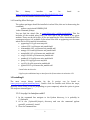
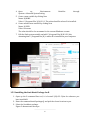
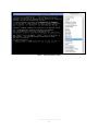
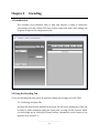
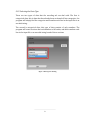
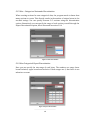
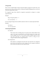
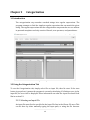
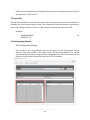
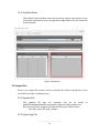
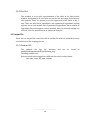
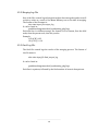
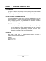
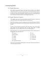
Gandhi Washington Method
Support Tool User Manual
SEDS Decision Support laboratory
University of Calgary
August 2015
1
Table of Contents
CHAPTER 1 – INSTALLATION ON WINDOWS
3
SECTION 1.1 REQUIREMENTS
SECTION 1.2 INSTALLING AND RUNNING THE GWM SUPPORT TOOL
SECTION 1.3 INSTALLING PYTHON
SECTION 1.4 INSTALLING THE REQUIRED PYTHON MODULES
SUBSECTION 1.4.1 INSTALLING PYQT5
SUBSECTION 1.4.2 INSTALLING WHEEL PACKAGES
SECTION 1.5 INSTALLING R
SUBSECTION 1.5.1 SETUP RPY2 TO INTERFACE WITH R
SUBSECTION 1.5.2 INSTALLING THE SCOTT KNOTT PACKAGE FOR R
3
3
4
4
4
4
5
5
6
CHAPTER 2 - ENCODING
7
SECTION 2.1 INTRODUCTION
SECTION 2.2 USING THE ENCODING TAB
SUBSECTION 2.2.1 SELECTING AN INPUT FILE
SUBSECTION 2.2.2 SELECTING THE DATA TYPE
SUBSECTION 2.2.3 NON-CATEGORICAL AUTOMATIC DISCRETIZATION
SUBSECTION 2.2.4 NON-CATEGORICAL EXPERT DISCRETIZATION
SECTION 2.3 INPUT FILE
SECTION 2.4 INTERPRETING RESULTS
SUBSECTION 2.4.1 RESULTS
SUBSECTION 2.4.2 FREQUENCIES
SECTION 2.5 OUTPUT FILES
SUBSECTION 2.5.1 RUNTIME FILE
SUBSECTION 2.5.2 OUTPUT LOG FILE
7
7
7
8
8
9
9
9
9
9
10
10
10
CHAPTER 3 - CATEGORIZATION
11
SECTION 3.1 INTRODUCTION
SECTION 3.2 USING THE CATEGORIZATION TAB
SUBSECTION 3.2.1 SELECTING AN INPUT FILE
SECTION 3.3 INPUT FILE
SECTION 3.4 INTERPRETING RESULTS
SUBSECTION 3.4.1 CATEGORIZED STRINGS
SUBSECTION 3.4.2 ARTIFICIAL NODES
SECTION 2.5 OUTPUT FILES
SUBSECTION 3.5.1 RUNTIME FILE
11
11
11
11
12
12
12
12
12
2
SUBSECTION 3.5.2 OUTPUT LOG FILE
12
CHAPTER 4 - SYNTHESIZING
13
SECTION 4.1 INTRODUCTION
SECTION 4.2 USING THE SYNTHESIZING TAB
SUBSECTION 4.2.1 SELECTING AN INPUT FILE
SECTION 4.3 INPUT FILE
SECTION 4.4 INTERPRETING RESULTS
SUBSECTION 4.4.1 FINAL RESULTS TABLE
SUBSECTION 4.4.2 BOX PLOT
SECTION 4.5 OUTPUT FILES
SUBSECTION 4.5.1 RUNTIME FILE
SUBSECTION 4.5.2 MERGING LOG FILE
SUBSECTION 4.5.2 FINAL LOG FILE
13
13
13
13
14
14
14
14
14
15
15
CHAPTER 5 – FITNESS OF STATISTICAL TESTS
16
SECTION 5.1 INTRODUCTION
SECTION 5.2 USING THE FITNESS OF STATISTICAL TESTS TAB
SUBSECTION 5.2.1 SELECTING AN INPUT FILE
SECTION 5.3 INPUT FILE
SECTION 5.4 INTERPRETING RESULTS
SUBSECTION 5.4.1 REGULAR EXPRESSIONS
SUBSECTION 5.4.2 REGULAR EXPRESSIONS PROPERTIES
SUBSECTION 5.4.2 STATISTICAL TESTS
16
16
16
16
17
17
17
18
3
Chapter 1
Installation on Windows
1.1 Requirements
The GWM Support Tool requires Python3.4 or above, various Python modules, the R
Project for Statistical Computing, and an additional R package. This program supports 32bit machines, but it should be noted that 64-bit machines must use 64-bit installations for
the dependencies.
This user manual only provides details for Windows operating systems, but the GWM
Support Tool can also run on Linux and Mac operating systems if all dependencies are in
place.









Python 3.4 or higher installed in the Path
PyQt5 python module
StatsModels python module
Numpy python module
Matplotlib python module
SciPy python module
Rpy2 python module
R 3.2.1 or higher installed in the Path
Scott Knott package for R
1.2 Installing and Running the GWM Support Tool
1. Get the zip file for the GWM Support Tool from a SEDS lab member.
2. Extract the zip file to any desired location.
3. Navigate to the extracted folder in the command line and run the command
python gw_method.py
1.3 Installing Python
The most recent binary installer for Python can be found at python.org/downloads/, select
a version higher than 3.4 and download the correct installer for your machine bit size.
Double click the installer and follow the steps, include Python in the path when the option
is given.
1.4 Installing the Required Python Modules
1.4.1 Installing PyQt5
4
The
binary
installer
can
be
http://sourceforge.net/projects/pyqt/files/PyQt5/PyQt-5.4.2/.
Double click the installer and follow the steps.
found
at
1.4.2 Installing Wheel Packages
The python packages should be installed via wheel files; this can be done using the
command:
python -m pip install WHEEL_FILE
in the command prompt.
You can find the wheel files at www.lfd.uci.edu/~gohlke/pythonlibs/. This list
includes all the needed wheel files; you can CTRL-F the file names in the given
website. These are the 64 bit files, if you are installing for 32bit, download the 32bit
counterpart above it if available. Some wheel files such as pyparsing use the same
wheel file for 32-bit and 64-bit machines:
 pyparsing-2.0.3-py3-none-any.whl
 cython-0.22.1-cp34-none-win_amd64.whl
 statsmodels-0.6.1-cp34-none-win_amd64.whl
 numpy-1.9.2+mkl-cp34-none-win_amd64.whl
 matplotlib-1.4.3-cp34-none-win_amd64.whl
 scipy-0.16.0b2-cp34-none-win_amd64.whl
 pandas-0.16.2-cp34-none-win_amd64.whl
 patsy-0.3.0-py2.py3-none-any.whl
 rpy2-2.6.0-cp34-none-win_amd64.whl
 pywin32-219-cp34-none-win_amd64.whl
* Install them in this order
* Rpy2 requires additional steps to interface with R, instructions in subsection 1.5.1
1.5 Installing R
The most recent binary installer for the R project can be found at
cran.r-project.org/bin/windows/base/. Double click the installer and follow the steps,
explicitly select 32-bit or 64-bit (depending on your computer) when the option is given.
The steps are shown Figure 1.
1.5.1 SetupRpy2 to Interface with R
1. In the command line navigate to the Python directory, it is probably in
C:\Python34
2. Go to the \Python34\Scripts\ directory and run the command python
pywin32_postinstall –install
3. Close the command line
5
4. Open
up
Environment
Variables
through
System > Advanced System Setting
5. Create a new variable by clicking New
Name: R_HOME
Value: C:\Program Files \R\R-3.2.1. The value should be where R is installed.
6. Create another new variable by clicking New
Name: R_USER
Value: Username
The value should be the username for the current Windows account.
7. Edit the Path system variable and add C:\Program Files\R\R-3.2.1\bin;
Assuming that C:\ProgramFiles\R\ is where R is installed on your computer.
Figure 1. Setting up R for GWM tool
1.5.2 Installing the Scott Knott Package for R
1. Open up the R command line tool, it is located \R\R-3.2.1\bin for wherever you
have installed R.
2. Enter the command install.packages() and pick the closest location to you.
3. Select the ScottKnott package.
Figure 2 demonstrate the steps.
6
Figure 2. Install Scott-Knott Package
7
Chapter 2
Encoding
2.1 Introduction
The encoding step translates lines of data and outputs a string of characters
representing each line of data. This step creates output that with a little editing can
be given as input to the categorization tab.
Figure3. Encoding tab
2.2 Using the Encoding Tab
To use the Encoding tab, first select an input file, change any settings you wish. Then
2.2.1 Selecting an Input File
An input file must first be specified in the Input File line in the Settings area. This can
be done by either manually typing the input path, or using the file browser which
can be brought up by clicking the Browse button. Information on the format of the
input file is in section 2.3.
8
2.2.2 Selecting the Data Type
There are two types of data that the encoding tab can deal with. The first is
categorical data, this is data that has already been sectioned off into categories, the
program will simply find the categories and translate each line in the input file to an
encoded string.
The second is categorical data; this type of data consists of only numbers. The
program will create sections that each number to fall under, and then translate each
line in the input file to an encoded string based of these sections.
Figure 4. Data type in encoding
9
2.2.3 Non – Categorical Automatic Discretization
When creating sections for non-categorical data, the program needs to know how
many sections to create. This directly results in the number of unique letters in the
encoded strings. You can specify between 2-5 sections using the discretization
option. Alternatively you can specify the range of each section yourself through the
Expert Discretization option; this is discussed in section 2.2.4.
Figure 5. Data discretization
2.2.4 Non-Categorical Expert Discretization
Here you can specify the size range of each letter. The numbers are range lower
bound inclusive, upper bound non-inclusive. If both ranges are 0, that letter is not
taken into account.
Figure 6. Expert discretization
10
2.3 Input File
There are two available kinds of input, categorical and non-categorical. In both cases, each
entry is on a new line, and there must be a numerical Gandhi Washington Factor at the end
of each line separated by a space.
For categorical input, there should be categories represented as strings in a comma
separated format.
Example:
Dog, Cat, Dog, Dog, Mouse
Cat, Cat, Cat, Mouse
5
2
For non-categorical input, there should be numerical values in a comma separated format.
Example:
5,2,2,3,8,9,9
1,2,1,1,1,3,4,2,9,8 10
4
2.4 Interpreting Results
2.4.1 Results
The results of the encoding process are given in the results window. Each
entry in the input is represented by an encoded string in the output, with
letters ranging from A to E in the encoded string. A legend is given for what
each letter represents, for categorical data, it will be a string, for noncategorical data it will be a range of numbers.
2.4.2 Frequencies
This window is a histogram of all the data in the input file. For categorical
data it shows the frequency of each category. For non-categorical numerical
data it shows the frequency of the numerical data.
11
2.5 Output Files
There is one output file created as well as another file which is updated for every
successful run of the encoding process.
2.5.1 Runtime File
The
updated
file
logs
the
runtimes
and
can
be
gandhiwashingtonmethod/encoding_pkg/encoding_runtimes.csv.
Each successful run is logged on a different line, and is in the format:
date time, input_file_path, runtime
found
at
2.5.2 Output Log File
The
other
file
created
can
be
found
in
gandhiwashingtonmethod/encoding_pkg/logs/. The format of the file name
is:
date time input_file output_log.
The log is in csv format, each line is a new entry, is in the format:
input_data encoded_expression GWF
The input_data is the same as that of the input file, with the difference of
being semi-colon separated.
12
Chapter 3
Categorization
3.1 Introduction
The categorization step matches encoded strings into regular expressions. The
program attempts to find the simplest regular expression that can match the given
string. The regular expressions that the categorization steps matches too are written
in premade templates and only consist of literals, star operators, and parentheses.
Figure 7. Categorization interface
3.2 Using the Categorization Tab
To use the Categorization tab, simply select file an input file, then hit start. If the start
button is greyed out, it means the program is currently calculating. If it finds an error in the
input file, an error will be displayed. More information on what the input file should look
like in section 3.3.
3.2.1 Selecting an Input File
An input file must first be specified in the Input File line in the Choose File area. This
can be done by either manually typing the input path, or using the file browser
13
which can be brought up by clicking the Browse button. Information on the format of
the input file is in section 2.3.
3.3 Input File
The input file should be a text file where each line is a new entry. Each line should have 2
columns, the first column being a string. The string should be alpha numeric and have no
more than 5 unique characters. The second column is an arbitrary numerical GWF.
Example:
AABBAAAABAD
DDESYSY 3.5
6.2
3.4 Interpreting Results
3.4.1 Categorized Strings
The results of the categorization process are given in the Categorized Strings
window. The first column is the input string. The second column is the regular
expression that the input string has been categorized into. The third column is the
distance of the regular expression from the root in a template.
Figure 8. Categorized strings
14
3.4.2 Artificial Nodes
The artificial nodes window shows the necessary regular expressions so that
the regular expressions in the categorized strings window are all connected
in the template.
Figure 8. Artificial nodes
3.5 Output Files
There is one output file created as well as another file which is updated for every
successful run of the encoding process.
3.5.1 Runtime File
The updated file logs the runtimes and can be found
gandhiwashingtonmethod/categorization_pkg/encoding_runtimes.csv.
Each successful run is logged on a different line, and is in the format:
date time, input_file_path, runtime
3.5.2 Output Log File
15
at
The
other
file
created
can
be
found
in
gandhiwashingtonmethod/encoding_pkg/logs/. The format of the file name
is:
date time input_file output_log
The log is in csv format, each line is a new entry, is in the format:
input_data encoded_expression GWF
The input_data is the same as that of the input file, with the difference of
being semi-colon separated.
16
Chapter 4
Synthesizing
4.1 Introduction
The goal of the synthesizing step is to merge separate regular expressions where
the Gandhi Washington Factors categorized into them are statistically different; we
determine this through the Mann-Whitney U-test. This is done by first selecting a
minimal sub hierarchy from a template that only contains nodes that have data
associated with them, and nodes that could potentially be needed in the merging
process. The step after is merging children to parents that are not statistically
different.
4.2 Using the Synthesizing Tab
To use the Synthesizing tab, simply select an input file, and then hit start. If the start
button is greyed out, it means the program is currently calculating. If it finds an
error in the input file, an error will be displayed. More information on what the
input file should look like in section 4.3.
4.2.1 Selecting An Input File
An input file must first be specified in the Input File line in the Choose File
area. This can be done by either manually typing the input path, or using the
file browser which can be brought up by clicking the Browse button.
Information on the format of the input file is in section 4.3.
4.3 Input File
Input should be in the format of a regular expression, followed by a series of
numbers, all of which are space separated.
Example:
A*B* 9 32 2 2.2 91 2
BABA 9 1 2 2 2 3.3 5
4.4 Interpreting Results
4.4.1 Final Results Table
The result of the merging process is given in the final results window. Each
row is a separate entry consisting of a pattern, the total items grouped into
that pattern, and the mean of all the items grouped into that pattern.
17
4.4.2 Box Plot
This window is a box plot representation of the table in the final results
window, by showing it in a box plot; we can also see the range of the items in
each pattern. There are options to set the upper and lower limits of the yaxis. There are also linear, logarithmic, and symmetrical logarithmic scaling
options; linear is the default scale. Symmetrical logarithmic can be treated as
logarithmic but with negative values included. Once the desired settings are
selected, click the update button to update the box plot.
4.5 Output File
There are two output files created as well as another file which is updated for every
successful run of the merging process.
4.5.1 Runtime File
The updated file logs the runtimes and can be found
gandhiwashingtonmethod/synthesizing_pkg/
encoding_runtimes.csv.
Each successful run is logged on a different line, and is in the format:
date time, input_file_path, runtime
18
at
4.5.2 Merging Log File
One of the files created logs what patterns have been merged together as well
as their p-value as a result of the Mann-Whitney test at the time of merging.
The format of the file name is:
date time input_file output_log
It can be found at:
gandhiwashingtonmethod/synthesizing_pkg/logs
Each new line is a different merge; the format is in csv format, first the child
node, then the parent node, then the p-value.
Example:
A*B, A*B*, 0.98
CB, (C*B*)*, 0.10
4.5.3 Final Log File
The final file created logs the results of the merging process. The format of
the file name is:
date time input_file final_output_log
It can be found at:
gandhiwashingtonmethod/synthesizing_pkg/logs
Each line is a pattern, followed by the final number of items in that pattern.
19
Chapter 5
Fitness of Statistical Tests
5.1 Introduction
The Fitness of Statistical Tests presents a series of statistical tests on data given in a
file. The format of the input file is the same as in the Synthesizing tab and so is
useful to verify certain results.
5.2 Using the Fitness of Statistical Tests Tab
To use the Synthesizing tab, simply select an input file, and then hit start. If the start
button is greyed out, it means the program is currently calculating. If it finds an
error in the input file, an error will be displayed. More information on what the
input file should look like in section 5.3.
5.2.1 Selecting an Input File
An input file must first be specified in the Input File line in the Choose File
area. This can be done by either manually typing the input path, or using the
file browser which can be brought up by clicking the Browse button.
Information on the format of the input file is in section 4.3.
5.3 Input File
Input should be in the format of a regular expression, followed by a series of
numbers, all of which are space separated.
Example:
A*B* 9 32 2 2.2 91 2
BABA 9 1 2 2 2 3.3 5
20
5.4 Interpreting Results
5.4.1 Regular Expressions
The regular expressions listed in the input file are placed in the Regular
Expressions windows. You can select them to view various information about
the data associated with that regular expression. The left and right windows
are identical, when both sides have a regular expression selected, there will
be a histogram showing the data for each regular expression.
5.4.2 Regular Expression Properties
The regular expression properties windows show the results of statistical
tests specifically for the regular expression selected above.
The KS Test Statistic is result of running the One-Sided Kolmogorov Smirnov
Normality Test on the data in the selected regular expression; this is not the
p-value.
P-Value is the p-value derived from the KS Test Statistic, any p-value above
0.05 accepts the null hypothesis that the data comes from a normal
distribution, any p-value below 0.05 rejects the null hypothesis.
Best Distribution is the closest matching distribution from a selected pool of
distributions. The selected pool is:











Uniform
Exponential
Gamma
Weibull
Normal
Beta
Logistic
Johnson SB
Johnson SU
Triangular
Logarithmic Normal
Total Items is the amount of data points in the input file associated with the
selected regular expression.
21
5.4.3 Statistical Tests
The statistical tests window contains two sections, the Scott Knott test
results, and the graphical distribution (along with other data).
The graphical distribution window can be activated by selecting a regular
expression from the left and right side windows. The regular expressions
must both have at least 2 data points to activate the graphing area. A TwoSided Kolmogorov Smirnov Test is also run between the data in the two
regular expressions, again showing the Kolmogorov-Smirnov Test Statistic,
and the resulting P-Value. A run time is also shown for how long it took to
run the individual tests (the two-sided tests are not included). You can
choose the number of sections in the histogram in the Bins option, once the
desired number of sections is written, click Update to update the graph. To
view the Scott Knott test results, click the "Scott Knott Results" button at the
bottom.
In the Scott Knott page, you can click the "Distributions" button to go back to
the previous page. The Scott Knott page shows the results from running the
Scott Knott test with all the regular expressions. Regular expressions are
categorized into ranks; regular expressions sharing the same rank are
grouped together in the Scott Knott test due to having similar data. The
means for each regular expression are also shown in this page.
22