Download CAIQS User's Guide

CAIQS program v. 1
1
28/02/03
CAIQS User’s Guide
1. Description
The program computes the adverse impact and the average quality of a (singlestage) large sample selection using a weighted predictor combination for either a given
set of overall selection ratios or a given set of majority group related selection ratios.
By default, the calculation of the adverse impact and the average quality is performed
for the following selection ratios: .01, .05, .10, .15, .20, .25, .30, .35, .40, .45, .50,
.55, .60, .65, .70, .75, .80, .85, .90, .95 and 1.00. For each selection ratio, the average
quality corresponds to the average score of the selected applicants on either the predictor
composite or a weighted combination of criterion dimensions. The average quality is
computed for (a) all the selected applicants, (b) the selected applicants from the majority
group and (c) the selected applicants from the minority group. When the computations
refer to the selection of a given overall selection ratio, then the results are reported
using two different metrics: (a) results standardized with respect to the distribution
(metric) of the total applicant population and (b) results standardized with respect
to the distribution (metric) of the majority group population. More specifically, using
µa ≡ 0 and µi for the average (composite) criterion (or predictor) score in the majority
group and the average (composite) criterion (or predictor) score in the minority group,
respectively, assuming that both applicant groups have the same (composite) criterion
(predictor) variance, σ ≡ 1 (see below), and given that the total applicant group consists
of a proportion, pa , of majority group candidates, and a proportion, pi , of minority group
applicants, the average score on the composite criterion (predictor) of the majority and
(s)
the minority group selected is, according to the first metric, expressed as
(s)
µi −µt
σt
µa −µt
σt
and
, respectively. In the above expressions, µt = pa µa + pi µi and σt2 = 1 + pa pi d2 ,
where d denotes the effect size of the composite criterion (predictor). In the second
(s)
(s)
metric, only the values µa and µi
(s)
the corresponding differences,
are reported. In addition to these average scores,
(s)
µa −µi
σt
(s)
(s)
and µa − µi
are presented as well. These
differences represent the effect size (expressed in the metric of σt and σ, respectively)
of the criterion (predictor) composite in the selected subgroup and these measures can
therefore be used to gauge the effect of prior selection on the subgroup differences found
in the selected group (cf. the paper by Roth et al., 2001).
The option to consider selections where the selection ratio refers to a given proportion
of the majority applicant group was added to provide results that cover those computed
by Bartram (1995). Also, in that case only the second metric is used to report the
average qualities of the majority and the minority selected candidates as well as the
difference between the two quantities.
Apart from performing the calculations for the given set of selection ratios, the
CAIQS program v. 1
2
28/02/03
program also determines the minimum value of the overall (or majority group related)
selection ratio for which the adverse impact ratio of the selection is no less than .800
(cf. the so-called four-fifths rule), and reports the average qualities (total, majority and
minority group selected) and the above documented effect sizes. In addition, the user
can complete the calculations for a limited number of still other (overall or majority
group related) selection ratios.
Finally, when the program is used to focus on a criterion (composite), the user can
(a) pre-specify the weights with which the predictors are combined to the predictor
composite or (b) let the program compute the regression based weights of the predictors
with respect to criterion (composite). Obviously, when the user focuses on the predictor
(composite), then only option (a) is available.
2. Assumptional Basis
The calculations are based on the assumption that the predictor and (eventually) the
criterion dimensions have a joint multivariate normal distribution with the same variance/covariance matrix but a different mean vector in the two applicant populations.
Given this assumption it is, without further restrictions, understood that the joint distribution of the predictors and the criterion dimensions is standard multivariate normal
in the majority applicant population.
The method is appropriate for large sample selections. The results are exact when
the number of applicants (both in the majority and the minority applicant group) tends
to infinity. For small(er) samples of applicants, the average quality results are only
approximate and typically overestimate the real expected values.
3. Technical Aspects
At present, the program is limited to situations where the total number of predictors and criterion dimensions is not greater than 10. The limitation is easily removed,
however.
To safely run the compiled program, a PC running under MS-Windows 95, 98, NT
or 2000 and with at least 64 MB RAM memory is required.
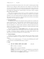
4. Input
• # 1: NP, NC, NVERH, NREG, NCR, NRSR
(6i3) with
– NP: the number of predictors
– NC: the number of criterion dimensions
– NVERH: when NVERH is set equal to 1, the calculations are performed for
overall selection ratios; whereas for NVERH = 0, the calculations pertain to
selection ratios for the majority applicant group
CAIQS program v. 1
3
28/02/03
– NREG: when NREG is equal to 0, the weights with which the predictors are
combined to the predictor composite is specified by the user. When NREG
= 1, the program computes the regression based weights for the predictors
with respect to the criterion composite. Observe that the latter option is
only feasible when NC is at least equal to 1.
– NCR: when NCR is set equal to 1, then the computed average qualities
pertain to the criterion composite; whereas for NCR equal to 0 the average
qualities refer to the predictor composite.
– NRSR: the number of additional selection ratios for which the user requests
the computation of adverse impact and average quality
• # 2: Optional only required when NVERH = 1. VERH
(f7.3)
VERH indicates the ratio between the size of the majority applicant group and
that of the minority applicant group.
• # 3: Optional only required when NREG = 0. WEP(I) with I = 1, ..., NP
(10f7.3)
The element WEP(I) indicates the weight with which the Ith predictor is used in
the predictor composite.
• # 4: Optional only required when NC 6= 0. WEC(I) with I = 1, ..., NC
(10f7.3)
The element WEC(I) indicates the weight with which the Ith criterion dimension
is used in the criterion composite.
• # 5 and following: CORIN(I,J) with both I and J ranging from 1 to NP + NC.
(7f7.3)
CORIN specifies the full correlation matrix between the predictors (first NP rows
and columns of the matrix) and the criterion dimensions (final NC rows and
columns of the matrix)
• # 6: DIFP(I) with I ranging from 1 to NP
(10f7.3)
The element DIFP(I) specifies the effect size of the Ith predictor. As the program
presumes that the average score of the predictors is zero in the majority applicant
population, the elements of the vector DIFP have typically a negative value. For
example, suppose that the difference between the average score on predictor 2
of the majority and the minority population (expressed relative to the common
standard deviation of the predictor in both populations) is 0.450, then the second
element of DIFP, DIFP(2) is set equal to -0.450.
CAIQS program v. 1
4
28/02/03
• # 7: Optional only required when NC 6= 0 DIFC(I) with I ranging from 1 to NC
(10f7.3)
The element DIFC(I) specifies the effect size of the Ith predictor. As the program
presumes that the average score of the predictors is zero in the majority applicant
population, the elements of the vector DIFC also have typically a negative value.
• # 8: Optional only required when NRSR 6= 0 RSR(I) with I ranging from 1 to
NRSR
(10f7.3)
The elements of RSR specify the selection ratios for which the user wants the calculation of the adverse impact and the average quality in addition to the selection
ratios that are analyzed by default.
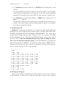
5. Sample Input File
Important: in preparing the input file, use a simple text editor such as Notepad,
Wordpad or any other standard ASCII producing editor. DO NOT USE TEXT PROCESSING PROGRAMS SUCH AS MS-WORD or WORDPERFECT. Also, when saving
the input file in Notepad, use the option “All Files” in the “Save as type” box. When
saving in Wordpad, use the “Text Document-MS-DOS Format” option in the “Save as
type” box, and be aware that Wordpad has the nasty habit of adding the extension .txt to the file name that you specify. Thus, with Wordpad, if you specify the
name of the input file as “MINPUT”, the file will in fact be saved as “MINPUT.TXT”;
and this is the name that you have to use in the command to run the present programs.
Here is a sample input file, for the caiqs program.
4
2
1
1
1
3
4.000
6.000
2.000
1.000
0.170
0.000
0.100
0.290
0.160
0.170
1.000
0.120
0.160
0.300
0.260
0.000
0.120
1.000
0.470
0.120
0.200
0.100
0.160
0.470
1.000
0.240
0.250
0.290
0.300
0.120
0.240
1.000
0.170
0.160
0.260
0.200
0.250
0.170
1.000
-1.000 -0.090 -0.090 -0.200
-0.450
0.000
0.075
0.250
0.320
6. Running the Program
Suppose you copied the executable source of the program to the d:publik directory
on your machine. In that case, the input file must also be saved in the d:publik
CAIQS program v. 1
5
28/02/03
directory. Next, to run the program, you have to open an MS-DOS Command window.
The way to do this varies from one operating system (i.e., Windows 95, 98, NT a.s.o.)
to the other, and you should use your local “HELP” button when in doubt about this
feature.
In the MS-DOS Command window you type d:, followed by RETURN or ENTER,
and your computer will return the D:\> command prompt. Next, you type cd publik
after the D:\> command prompt, again followed by RETURN or ENTER, and your
computer will respond with the D:\publik> command prompt. Now, you can execute
the program by typing caiqs < minput > moutput
where “minput” is the name
of the input file and “moutput” is the name of the output file. At the end of the
execution, the PC will return the command prompt D:\publik>. You can then inspect
the output by editing the output file with either Notepad, Wordpad or any other simple
editor program.
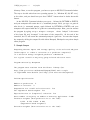
7. Sample Output
Computing adverse impact and average quality of the selected subjects
(with respect to either a criterion or a predictor composite)
of a selection using a weighted predictor combination
for a given overall or majority group related selection ratio
Program written by Anonymous
The program uses routines from the Slatec library (see
http://www.geocities.com/Athens/Olympus/5564) and a couple
of algorithms from StatLib (see http://lib.stat.cmu.edu/apstat/)
Problem specification
Number of predictors:
Number of criteria:
4
2
Computation for overall selection ratio: Yes
Use regression based weights: Yes
Expected scores on (composite) criterion: Yes
Ratio number of majority vs number of minority applicants: 4.000
Predictor weights (from predictor one to the last):
0.244
0.270
0.039
0.206
(Regression based weights!)
Criterion weights (from criterion one to the last):
CAIQS program v. 1
6.000
6
28/02/03
2.000
Effect sizes (i.e., standardized difference between the
minority and the majority group) of the predictors
-1.000 -0.090 -0.090 -0.200
Effect sizes (i.e., standardized difference between the
minority and the majority group) of the criteria
-0.450
0.000
Correlation matrix of the predictors (first 4 rows and columns)
and the criteria (final 2 rows and columns)
Row
1
1.000
0.170
0.000
0.100
0.290
0.160
Row
2
0.170
1.000
0.120
0.160
0.300
0.260
Row
3
0.000
0.120
1.000
0.470
0.120
0.200
Row
4
0.100
0.160
0.470
1.000
0.240
0.250
Row
5
0.290
0.300
0.120
0.240
1.000
0.170
Row
6
0.160
0.260
0.200
0.250
0.170
1.000
Correlation between weighted predictor and weighted
criterion combinations:
Squared correlation:
0.487
0.237
Effect size predictor composite -0.643
Effect size criterion composite -0.407
Minimum overall selection ratio without AI 4/5th rule is
0.846
with selection ratio majority and minority group equal
to
0.881
0.705 , respectively
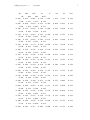
For each overall selection ratio (SR): the majority group SR (SRA)
the minority group SR (SRI), the adverse impact (AI), the overall
average quality of the selected individuals (with respect to
the majority group distribution: wrtmgd) (M), the average quality
of the majority group selected {wrtmgd) (MA) and the minority
group selected (again wrtmgd) (MI), and the
difference between
MA and MI.
On the second line: the globally standardized (gs) overall average
quality of the selected individuals (SM), the (gs) average quality of the
majority selected individuals (SMA), the (gs) average quality of the
minority selected (SMI) and the difference between SMA and SMI (SDIF)
CAIQS program v. 1
SR
SRA
SM
0.010
1.326
0.050
1.030
0.100
0.879
0.150
0.779
0.200
0.703
0.250
0.639
0.300
0.583
0.350
0.533
0.400
0.487
0.450
0.444
0.500
0.403
0.550
0.364
0.600
0.326
0.650
0.289
0.700
0.252
0.750
0.215
0.800
0.178
0.850
SRI
SMA
0.012
0.117
0.033
0.888
0.173
0.057
0.791
0.229
0.083
0.715
0.284
0.113
0.653
0.339
0.145
0.599
0.393
0.180
0.551
0.446
0.218
0.506
0.498
0.259
0.465
0.549
0.302
0.426
0.600
0.349
0.389
0.650
0.399
0.354
0.699
0.452
0.319
0.748
0.510
0.286
0.795
0.571
0.252
0.840
0.638
0.219
0.885
0.711
0.148
0.644
0.489
0.154
0.581
0.420
0.161
0.526
0.359
0.167
0.477
0.303
0.174
0.432
0.251
0.181
0.390
0.202
0.188
0.351
0.155
0.195
0.313
0.110
0.204
0.277
0.065
0.213
0.242
0.020
0.223
0.208
-0.026
0.234
0.174
-0.072
0.247
0.141
-0.121
0.262
0.107
-0.173
0.280
0.631
0.566
0.510
0.459
0.412
0.368
0.327
0.287
0.249
0.211
0.174
0.137
0.243
0.759
-0.039
0.572
0.231
0.719
0.009
0.720
0.708
0.220
0.682
0.055
0.141
0.210
0.647
0.100
0.678
0.201
0.613
0.144
0.818
0.809
0.193
0.581
0.188
0.132
0.185
0.550
0.234
0.837
0.178
0.519
0.280
0.969
0.962
0.171
0.489
0.328
0.120
0.165
0.459
0.379
1.147
0.159
0.428
0.434
1.267
0.152
0.396
0.495
1.262
0.146
0.363
0.563
DIF
0.139
0.327
0.645
MI
0.131
0.285
0.749
MA
0.119
0.232
0.907
M
SDIF
0.156
1.212
0.014
1.037
AI
SMI
0.002
1.331
0.059
7
28/02/03
0.099
0.258
0.804
0.060
CAIQS program v. 1
0.140
0.900
0.186
0.927
0.099
0.950
0.056
1.000
0.000
0.080
0.073
-0.230
0.303
-0.025
0.037
-0.299
0.336
0.000
-0.407
0.407
0.332
1.000
-0.321
0.019
0.299
0.914
-0.214
1.000
0.276
0.854
-0.147
0.883
0.117
1.000
-0.090
0.792
0.152
0.967
8
28/02/03
-0.081
0.401
Details for minimum possible overall SR without AI
0.846
0.881
0.143
0.705
0.188
0.800
-0.086
0.063
0.110
-0.168
0.278
0.883
0.746
0.137
0.581
0.420
0.161
0.506
0.336
0.170
0.274
Details for requested overall selection ratios
0.075
0.088
0.944
0.250
0.952
0.284
0.639
0.320
0.023
0.360
0.563
0.817
0.113
0.653
0.566
0.159
0.440
0.412
0.875
0.135
0.396
0.495
0.159
0.579
0.261
0.489
0.168
8. Description of Output
The output is largely self-explanatory. Suffice it to restate that the average qualities
labeled as SM, SMA, SMI and the difference SDIF refer to the solution values that correspond to the earlier discussed metric of global standardization; whereas the quantities
M, MA, MI and DIF represent the average scores and the difference as obtained for the
standardization with respect to the majority applicant group.
9. Dependencies and Acknowledgment
The present program is written in Fortran77. It was compiled to an executable code
for WIN32 PCs (ie, Windows 95/98/ME or NT/2000) with the GNU Fortran G77 compiler (cf. http://www.geocities.com/Athens/Olympus/5564/). The program uses
routines from the SLATEC program library (cf. Fong et a., 1993;
http://www.geocities.com/Athens/Olympus/5564/) and a couple of algorithms
from StatLib
http://lib.stat.cmu.edu/apstat/).
When the user reports results obtained by the present program, due reference should be made to De Corte (2003), and De Corte & Lievens (2003).
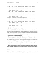
11. References
De Corte, W. (2003). Caiqs User’s Guide. http://allserv.rug.ac.be/~wdecorte/software.html
CAIQS program v. 1
28/02/03
9
De Corte, W., & Lievens, F. (2003). A practical procedure to estimate the quality
and the adverse impact of single-stage selection decisions. International Journal
of Selection and Assessment, 11, 89–97.
Bartram, D. (1995). Predicting adverse impact in selection testing. International
Journal of Selection and Assessment, 3, 52–61.
Fong, K. W., Jefferson, T. H., Suyehiro, & Walton, L. (1993). Guide to the SLATEC
common mathematical library (http://www.netlib.org/slatec/).
Roth, P. L., Bobko, P., Switzer, F. S. III, & Dean, M. A. (2001). Prior selection causes
biased estimates of standardized ethnic group differences: simulation and analysis.
Personnel Psychology, 54, 591–617.