Download AnalysisFW - User Manual

AnalysisFW - User Manual
Nicolas Lurkin
February 26, 2013
Abstract
AnalysisFW is a framework that has been written to provide tools to analyze data
coming from the ocial NA62 framework (NA62MC, NA62Reconstruction). These
data can be raw MC data, reconstructed MC data or reconstructed real data. It has been
designed in a modular way. A core part is taking care of all the initialization, reading of
data and providing tools to take advantage of the modularity. Other parts called analyzer
are simple processing units that can be written by the users and easily shared in the collaboration. Each of these analyzer can be included in the analysis through a conguration le.
The rst part of this document is intended to provide the user with the basic instruction to
begin to work with the framework. The second part provides information on how to write
new analyzers and what are the available built-in tools to help you. The last part can help
the user understand how the framework is internally working.
1
Contents
1 Quickstart
3
1.1
Conguration le . . . . . . . . . . . . . . . . . . . . . . . . . . . . . . . . . . . .
3
1.2
build_AnalysisFW.py
4
. . . . . . . . . . . . . . . . . . . . . . . . . . . . . . . . .
2 Using the FW
4
2.1
Writing a new analyzer . . . . . . . . . . . . . . . . . . . . . . . . . . . . . . . . .
2.2
Methods availables in the analyzer
4
. . . . . . . . . . . . . . . . . . . . . . . . . .
6
2.2.1
In Constructor
. . . . . . . . . . . . . . . . . . . . . . . . . . . . . . . . .
6
2.2.2
In InitHist() . . . . . . . . . . . . . . . . . . . . . . . . . . . . . . . . . . .
6
2.2.3
In InitOutput() . . . . . . . . . . . . . . . . . . . . . . . . . . . . . . . . .
7
2.2.4
In DeneMCSimple()
7
2.2.5
In Process() . . . . . . . . . . . . . . . . . . . . . . . . . . . . . . . . . . .
8
2.2.6
In ExportPlot() . . . . . . . . . . . . . . . . . . . . . . . . . . . . . . . . .
10
2.2.7
In DrawPlot()
. . . . . . . . . . . . . . . . . . . . . . . . . . . . .
. . . . . . . . . . . . . . . . . . . . . . . . . . . . . . . . .
10
2.3
Running the FW . . . . . . . . . . . . . . . . . . . . . . . . . . . . . . . . . . . .
10
2.4
Structure of the output le
11
. . . . . . . . . . . . . . . . . . . . . . . . . . . . . .
3 FW in depth
11
3.1
BaseAnalysis
. . . . . . . . . . . . . . . . . . . . . . . . . . . . . . . . . . . . . .
12
3.2
Analyzer . . . . . . . . . . . . . . . . . . . . . . . . . . . . . . . . . . . . . . . . .
12
3.3
MCSimple . . . . . . . . . . . . . . . . . . . . . . . . . . . . . . . . . . . . . . . .
13
3.4
DetectorAcceptance
14
. . . . . . . . . . . . . . . . . . . . . . . . . . . . . . . . . .
2
1
Quickstart
1. Make sure the following softwares are already installed. The versions indicated here are
the ones that have been tested but other versions might work as well.
•
•
•
•
•
•
gcc (4.6.3, 4.1.2)
Python (2.7)
ROOT (5.34.04)
Geant4 (4.9.5.p02)
NA62MC (rev 245, 255)
NA62Reconstruction (rev 245, 255)
2. Get the sources at http://nicolaslurkin.eu/svn/AnalysisFW/trunk (or /tags for stable version)
3. The following environment variables have to be set beforehand:
•
NA62MCSOURCE : should point to where is the source code of NA62MC
In addition, the ROOT and Geant4 install should be properly congured. Beware to always
use the same version of ROOT, Geant4, NA62MC and NA62Reconstruction as the ones
that were used to generate and reconstruct the data or strange behaviors might be observed.
4. Create a work directory where the personal code will be stored and compiled.
5. Create the required structure in the work directory with
./build_AnalysisFW.py prepare pathToWorkDirectory
6. Go in the work directory, verify the env.sh and source it.
7. Edit the cong le (section 1.1) to select the analyzers that needs to run/
8. Build the Framework with :
build_AnalysisFW.py config
(see section 1.2 for usage of build_AnalysisFW.py )
9. Run
./executable -i inputFile.root -o outputFile.root -v 1
1.1 Conguration le
The conguration le is very simple and allows to have dierent congurations with a single
instance of the code.
A conguration is dened by two elements :
•
analyzers : A list of analyzers to run
•
exec : The name for the generated executable
Analyzer folder of the
Examples folder of the FW) and user analyzers (located
The list of analyzers can contain ocial FW analyzers (located in the
FW), example analyzers (located in the
in the
Analyzer folder of the work directory).
3
1.2 build_AnalysisFW.py
build_AnalysisFW.py is a python script used to perform the basic operations with the FW. The
available commands are the following :
•
build_AnalysisFW.py help : will print the help of the build_AnalysisFW.py script
•
build_AnalysisFW.py available : will return the list of available Analyzers
•
build_AnalysisFW.py cleanUser : will remove all les generated by the build in the user
directory"
•
build_AnalysisFW.py cleanFW : will remove all les generated by the build in the FW
directory"
•
build_AnalysisFW.py new AnalyzerName : will create a new analyzer with name AnalyzerName in the user directory
•
build_AnalysisFW.py rename oldName newName : will rename a user analyzer
•
build_AnalysisFW.py congFileName :
will build the FW using the conguration le
congFileName
•
2
build_AnalysisFW.py prepare path : will prepare a user directory at the specied path
Using the FW
2.1 Writing a new analyzer
To write a new analyzer in the work directory :
1. Go in the work directory and source env.sh
2. Create a new analyzer with
build_AnalysisFW.py new analyzerName
3. Write the analyzer. The header and source les are
workDir/Analyzer/include/analyzerName.hh
workDir/Analyzer/src/analyzerName.cc
The analyzer derives from a base class that already provide some convenient methods to take
advantage of the FW. The user only have a minimum number of methods to ll.
The basic
code to be written in each one is described here. The Pi0Reconstruction analyzer is a working
example that can be found in the
Examples directory of the framework.
The rst 4 are initialization methods called when the class is instanciated :
•
Constructor : In this method, just specify which trees have to be loaded from the input
root le and which class is expected.
If needed, a DetectorAcceptance instance can be
requested or created (see section 3.4).
•
InitHist : All the histograms that will be used in the analyzer should be booked here with
4
BookHisto(name, histoPtr);
They will be made available everywhere in the analyzer through
FillHisto(name, value[, value, [value]]);
fHisto[name];
fHisto2[name];
fGraph[name];
In addition they will easily be saved in the output le later with
SaveAllPlots();
Or drawn with
DrawAllPlots();
•
InitOutput : If some values have to be made available to other analyzer, they must be
registered in this function with
RegisterOutput(name, &variable);
The variable has to be declared as member of the class in the header le and a pointer to
this variable has to be passed to the function. The name will be prepended with the name
of the analyzer to avoid collisions.
Any output variable can be used in any other analyzer by using the following syntax :
outputType var = *(outputType*)GetOutput("analyzerName.outputName", state);
where state is of type outputState.
Parameters for the analyzer can also be dened with
AddParam("paramName", "paramType", &variable, defaultValue);
This parameter can be set at runtime with the -p option. The syntax is dened in section
2.3
•
DeneMC : In this method, the required structure for the MC events in the MCSimple
class is dened :
int particleID = fMCSimple->AddParticle(parentID, pdgCode)
The 2 main processing methods called for each event :
•
Process : Main processing method, this is where the main code for the analysis shoud be
written.
•
Postprocess : This method is called after each event, once the Process method has been
called for each analyzer.
This is where the memory allocated for the output variable in
Process can be freed.
And 2 nalization methods called before terminating the program :
5
•
ExportPlot : All the histograms booked in InitHist can be written in the output le here.
It can be done for each histogram individually by calling the usual ROOT Write() method
or they can be all saved automatically by calling SaveAllPlots().
•
DrawPlot : If running interactively, all the histograms booked in InitHist can be drawed on
screen. It can be done for each histogram individually, using the usual ROOT way (canvas,
Draw() ), or calling DrawAllPlots() that will print them all automatically.
2.2 Methods availables in the analyzer
2.2.1 In Constructor
RequestTree(TString name, TDetectorVEvent *evt)
Request a new TTree containing
MC/Reconstructed events to be read from the input ROOT le.
name is the name of the tree as in the ROOT le.
evt is a pointer to a TDetectorVEvent instance.
Example :
RequestTree("GigaTracker", new TGigaTrackerEvent);
RequestTree("GigaTracker", new TRecoGigaTrackerEvent);
GetDetectorAcceptanceInstance()
Returns a pointer to the global instance of DetectorAc-
ceptance. This instance is unique for performances reasons as loading the geomtry le can take
up to 1 minute. It's still possible to create a local instance if needed (for specic geometry, ...).
Example :
//Global instance
fGeom = GetDetectorAcceptanceInstance();
//local instance
fGeom = new DetectorAcceptance("geometryFileName.gdml");
2.2.2 In InitHist()
BookHisto(TString name, TH1* histo)
Book 1D histograms and make them available in
the whole analyzer.
name is the name of the histogram that will be used later to refer to it.
histo is a pointer to the histogram.
Example :
BookHisto("VertexX", new TH1I("VertexX", "Reconstructed vertex X position", 100, 0, 300));
BookHisto(TString name, TH2* histo)
Book 2D histograms and make them available in
the whole analyzer.
name is the name of the histogram that will be used later to refer to it.
histo is a pointer to the histogram.
Example :
BookHisto("g1Reco", new TH2I("g1Reco", "g1 Reco vs. Real", 100, 0, 75000, 100, 0, 75000));
6
BookHisto(TString name, TGraph* histo)
Book graphs and make them available in the
whole analyzer.
name is the name of the graph that will be used later to refer to it.
histo is a pointer to the graph.
Example :
BookHisto("PhotonEfficiency", new TGraph());
2.2.3 In InitOutput()
RegisterOutput(TString name, void* address)
To make an output variable available in
all other analyzers, it needs to be registered with this method.
name is the name that will be used to refer to this variable in the other analyzer.
This name
will be prepended with the name of the analyzer.
address is a pointer to the output variable that has been declared as class member in the header
le.
Example :
RegisterOutput("vertex", &vertex);
AddParam(TSting name, TString type, T *variable, T defaultValue); Analyzers can
be parameterized. This method allows the user to add new parameters. name is the name that
will be used to set this parameter.
type is the type of parameter.
The possible values are bool, int, long, oat, double, char, string,
TString
variable is a pointer to the variable that has been declared as class member in the header le.
defaultValue the default value for the parameter if not specied at runtime.
Example :
int pdgType;
AddParam("ParticleType", "int", &pdgType, 321);
2.2.4 In DeneMCSimple()
fMCSimple->AddParticle(int parentID, int pdgCode)
Fill the MC event structure.
This method returns the ID of the particle in the structure.
parentID is the id of the parent particle.
pdgCode is the PDG code of the particle.
Example :
Structure for the decay
K + − > π + π 0 − > γγ .
Request an initial kaon from the beam, the
positive and neutral pions originating from this kaon and the two photons from the neutral pion
decay.
int kID = fMCSimple->AddParticle(0, 321); //ask for beam Kaon
fMCSimple->AddParticle(kID, 211); //ask for positive pion from initial kaon decay
int pi0ID = fMCSimple->AddParticle(kID, 111); //ask for neutral pion from initial kaon decay
fMCSimple->AddParticle(pi0ID, 22); //ask for photon from neutral pion
fMCSimple->AddParticle(pi0ID, 22); //ask for photon from neutral pion
7
2.2.5 In Process()
fMCSimple.status Returns the status of the MCSimple structure.
The values can be one of
the following :
•
MCSimple::kEmpty : when there is no MC data (example : for real data)
•
MCSimple::kMissing : MC data is present but the requested structure was not or partially
found.
•
MCSimple::kComplete : MC data is present and the requested structure was entirely found.
This state allows to distinguish between simulated/real events and to know if something happened
in the simulated event (Example : kMissing can arise when there was an inelastic interaction
between the beam kaon and a GTK station). It's up to the user to choose if the analyzer is able
to continue without complete MC data or to dene an alternate processing (Example : same
processing on real data and simulated ones but no comparison between reco and MC in the latter
case).
fMCSimple[TString particleName]
This can be used to get the information stored in the
MCSimple structure. This operator return a std::vector<KinePart*>. The particles are ordered
by id in the vector (see 2.2.4).
particleName is the name of the requested particle :
kaon, gamma, pi+, . . .
Example : Get Initial Energy of the rst gamma comming from the
π0
in the example structure dened in 2.2.4.
fMCSimple["gamma"][0]->GetInitialEnergy()
fMCSimple[int pdgCode]
This can be used to get the information stored in the MCSimple
structure. This operator return a std::vector<KinePart*>. The particles are ordered by id in
the vector (see 2.2.4).
pdgCode is the PDG id of the requested particle :
321, 22, 211, . . .
Example : Get Initial Energy of the rst gamma comming from the
π0
in the example structure dened in 2.2.4.
fMCSimple[22][0]->GetInitialEnergy()
GetEvent("treeName")
Get the event from the TTree. It need to be explicitely cast into
the right type.
treeName is the name of the Event as in 2.2.1
Example :
TRecoGigaTrackerEvent *GTKEvent = (TRecoGigaTrackerEvent*)GetEvent("GigaTracker");
8
fHisto["histoName"]
Returns the 1D histogram. If the requested histogram name does not
exist or is in another container, the program will segfault (to ll histograms, use FillHisto instead).
histoName is the name of the histogram as dened in 2.2.2
Example :
fHisto["VertexX"]->Draw();
fHisto2["histoName"]
Returns the 2D histogram.
If the requested histogram name does
not exist or is in another container, the program will segfault (to ll histograms, use FillHisto
instead).
histoName is the name of the histogram as dened in 2.2.2
Example :
fHisto["g1Reco"]->Draw();
fGraph["histoName"]
Returns the TGraph. If the requested histogram name does not exist
or is in another container, the program will segfault (to ll histograms, use FillHisto instead).
histoName is the name of the histogram as dened in 2.2.2
Example :
fHisto["PhotonEfficiency"]->Draw();
FillHisto(TString name, value[, value[, value]])
Fill histogram. The value arguments can
have the same signature as in the Fill() method of TH1, TH2 and TGraph.
name is the name of the histogram as dened in 2.2.2, 2.2.2 or 2.2.2
Example :
FillHisto("g1Reco", g1->GetInitialEnergy(), fMCSimple["gamma"][iLead]->GetInitialEnergy());
GetOutput(TString name, outputState &state)
This function returns a pointer to the
output variable of an analyzer. You have to cast it to the right type.
name is the name of the
output variable to request with the format "analyzerName.outputName", where analyzerName is
the name of the analyzer creating this output and outputName is the name given when registering
the variable (see 2.2.3).
state
is lled by the function with the state of this output variable.
It can take one of the
following values :
•
kOUninit : the variable has not been lled by the analyzer
•
kOValid : the variable has been lled by the analyzer and can be considered valid
•
kOInvalid :
the variable has been lled by the analyzer and can be considered invalid
(Example : Pi0Reconstruction tried to reconstruct a
π0
candidate from detected photons but found a bad invariant mass. The candidates can be
tagged as kOInvalid because the photons may not come from a
π0
)
9
Example :
TVertex3 vertex = *(TVector3*)GetOutput("VertexCDA.vertex", state);
SetOutputState(TString name, outputState state)
Set the state of the output variable.
The state is reset to kOUninit before each event and has to be set to the right value in the
analyzer.
name is the name of the output as in 2.2.3 (the name of the analyzer will be prepended to this
name).
state is the state to set.
Can be one of the following : kOUninit, kOValid, kOInvalid
Example :
SetOutputState("vertex", kOValid);
ExportEvent()
Events can also be exported in the output root le. If requested, the input
TTrees are copied in the output le and all the event for which this method is called are saved
in the output tree. The TTrees present in the input les are not copied if not requested by any
analyzer. An event is exported if at least one analyzer requests it.
2.2.6 In ExportPlot()
SaveAllPlots() This function will write in the output ROOT le all the plots that have been
booked with BookHisto.
2.2.7 In DrawPlot()
DrawAllPlots(); This function will draw on the screen all the plots that have been booked
with BookHisto.
2.3 Running the FW
To run the program with a set of analyzers
1. Go in the work directory and source env.sh
2. Create a cong le containing the name of the executable and the list of analyzer to run
separated by white spaces. Dierent conguration les can be created and thus dierent
executables can exist simultaneously.
exec = executableName
analyzers = analyzer1 analyzer2 analyzer3
3. Compile with
build_AnalysisFW.py configFileName
4. Run with
./executableName -i InputFile | -I InpuFilesList [-n FirstEvent]
[-N NumberOfEvents] [-o OutputFile] [-v verbosity]
[-p "analyzer:param=val;param=val&analyzer:param=val&..."] [-h]
10
•
-i : Path to the input ROOT le. When running on a single ROOT le.
•
-I : Path to a text le where each line contains a path to a ROOT le. When running on
multiple ROOT les.
•
-n : First event to process. Skip the n-1 rst events. Very rst event is number 0 (default)!
•
-N : Total number of events to process. Default : total number of events in the les. The
total number of events processed is then N-n.
•
-o : Path to the output le (will be overwritten if already exists). Default : outputFile.root
•
-v : verbosity (only used by MCSimple so far)
•
-p : Parameters for the analyzers
•
-h : Print this help
2.4 Structure of the output le
In the output le, a folder is created for each analyzer. The SaveAllPlots() function will save all
the booked histograms and graphs into the correct folder.
3
FW in depth
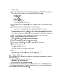
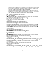
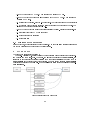
The framework is structured as follow :
The build_AnalysisFW.py script will read the conguration le and generate the correspond-
BaseAnalysis, the
Analyzer) and load them in
BaseAnalysis in the correct order (dependencies). For each loaded analyzer, BaseAnalysis
will create an instance of MCSimple. Some analyzers can freely create an instance of DetectorAcceptance.
ing Makele and the main.cc le. This main.cc will create an instance of
instances of each required analyzers (deriving from base class
Figure 1: Structure of the Framework
11
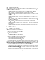
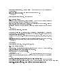
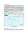
3.1 BaseAnalysis
This class is the central point in the framework. It contains all the analyzers and an instance of
MCSimple for each, all the output from each analyzer and their current state. It can instantiate
the unique global DetectorAcceptance class
It takes care of loading and decoding the input root les, initializing the analyzers and
MCSimple, creating the output root le, parsing and setting the parameters for each analyzer.
The input TTrees are then read and processed event by event. In the event loop, each MCSimple
instance will search the MC data to nd the event structure that has been requested.
The
output state of each analyzer will be reset and then each one will be processed in turn.
The
ordering matters because some analyzers can use the output of a previous analyzer. Once all the
analyzers have been processed, a post-processing method is called for eventual operations like
freeing memory allocated for the output (Example : the output is a list of
vector<KinePart*>).
π0
candidates of type
BaseAnalysis will draw the plots on screen in case
-o option) and export them in the output root le.
Once all the events have been processed, the
of interactive running (without the
Figure 2:
BaseAnalysis class
3.2 Analyzer
This is the virtual base class for all analyzers. Some initialization steps are already done here as
well as the complete pre-processing step. Number of methods to help the user writing his own
12
analyzer are provided here :
•
void BookHisto(TString name, TH1* histo)
•
void BookHisto(TString name, TH2* histo)
•
void BookHisto(TString name, TGraph* histo)
•
void FillHisto(TString name, TString x, int w)
•
void FillHisto(TString name, double x, int w)
•
void FillHisto(TString name, double x)
•
void FillHisto(TString name, double x, double y, int w)
•
void FillHisto(TString name, double x, double y)
•
void RequestTree(TString name, TDetectorVEvent* evt)
•
void DrawAllPlots()
•
void SaveAllPlots()
•
void RegisterOutput(TString name, void* address)
•
void SetOutputState(TString name, OutputState state)
•
void *GetOutput(TString name, OutputState &state)
•
DetectorAcceptance *GetDetectorAcceptanceInstance()
•
void ExportEvent();
•
TDetectorVEvent *GetEvent(TString name);
•
void AddParam(TString name, TString type, T* address, T defaultValue)
For the description of the methods listed here, please refer to section 2.2
3.3 MCSimple
This class is intended to provide an easy way to dene what kind of events should be extracted
from MC and provides an easy access to this smaller set of information. It doesn't replace the
complete MC event as it still possible to access the complete information through MCTruthEvent
in the processing method of the analyzer. It provides the following methods :
•
int AddParticle(int parent, int type)
•
vector<KinePart*> operator[](TString)
•
vector<KinePart*> operator[](int)
For the description of the methods listed here, please refer to section 2.2
13
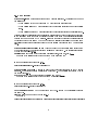
3.4 DetectorAcceptance
This class provides an easy way to check acceptance with the geometry implemented in NA62MC.
This geometry is loaded from a
.gdml le created by NA62MC. After giving the startpoint and
the direction of a track, this class will check which detector volumes are crossed by the track and
which one is the rst. It provides the following methods :
When executing the following methods, the class will modify the values of the internal structure :
•
void FillPath(TVector3 position, TVector3 momentum, double precision) : Set true for
each crossed detector and each station and plane in GTK, LAV, Spectrometer. Set also
the corresponding position.
The results of this method can then be retrieved with the
following methods. Precision is the length of each step.
•
void FillPath(TVector3 position, TVector3 momentum) : Set true for each crossed detector and each station and plane in GTK, LAV, Spectrometer. Set also the corresponding
position. The results of this method can then be retrieved with the following methods.
•
void CleanDetPath() : Reset the internal structure for a new track.
The following methods can be used to retrieve the values in the internal structure :
•
bool GetDetAcceptance(volume det) : Return true if the path cross the specied volume.
•
TVector3 GetDetPosition(volume det) : Return the position where the path crossed the
specied volume (if crossed)
•
bool GetGTKAcceptance(GTKVol det) : Return true if the path cross the specied GTK
volume.
•
TVector3 GetGTKPosition(GTKVol det) : Return the position where the path crossed the
specied GTK volume (if crossed)
•
bool GetStrawAcceptance(StrawVol det) : Return true if the path cross the specied Straw
volume.
•
TVector3 GetStrawPosition(StrawVol det) : Return the position where the path crossed
the specied Straw volume (if crossed)
•
bool GetLAVAcceptance(LAVVol det) : Return true if the path cross the specied LAV
volume.
•
TVector3 GetLAVPosition(LAVVol det) : Return the position where the path crossed the
specied LAV volume (if crossed)
•
volume FirstTouchedDetector() : Return the rst volume to be crossed by the path
•
•
volume CheckDetectorAcceptPoint(Double_t x,Double_t y, Double_t z) : Say in which
volume the given point is located.
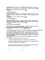
The following methods are used for display :
•
void DrawDetector() : Display a 3D drawing of the detector
14
•
void CreateTrack(int pdgID,TVector3 position, TVector3 momentum, int charge) : Create
a new track in the detector (for display only)
•
void DrawTracks() : Display all the existing tracks created with CreateTrack
•
void ClearTracks() : Remove all the tracks created with CreateTrack
•
void DrawPoint(double x, double y, double z) : Display a point at the given position on
the 3D drawing.
In addition some enum are set to identify the volumes
•
enum volume kCEDAR, kGTK, kCHANTI, kLAV, kSpectrometer, kIRC, kCHOD, kLKr,
kSAC, kMUV1, kMUV2, kMUV3, kVOID
•
enum GTKVol kGTK0, kGTK1, kGTK2, kNOGTK
•
enum StrawVol kSTRAW0, kSTRAW1, kSTRAW2, kSTRAW3, kNOSTRAW
•
enum LAVVol kLAV0, kLAV1, kLAV2, kLAV3, kLAV4, kLAV5, kLAV6, kLAV7, kLAV8,
kLAV9, kLAV10, kLAV11, kNOLAV
15