Download ULTRASONIC SIGNAL PROCESSING TOOLBOX User Manual v1.0

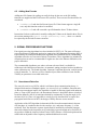
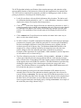
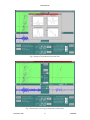
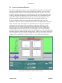
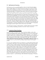
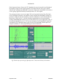
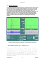
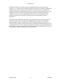
ULTRASONIC SIGNAL PROCESSING TOOLBOX
User Manual v1.0
Acknowledgment
The authors would like to acknowledge the financial support of European
Commission within the project SPIQNAR FIKS-CT-2000-00065
copyright
Lars Ericsson
Uppsala University
Signals and Systems
September 2001
Disclaimer
The Ultrasonic Signal Processing Toolbox (USPT) can be used for
research purposes only. It is distributed in the hope that it will be useful
for the research community but WITHOUT ANY WARRANTY.
More specifically:
THE PROGRAM IS PROVIDED “AS-IS” WITHOUT WARRANTY OF ANY KIND,
EITHER EXPRESS OR IMPLIED, INCLUDING BUT NOT LIMITED TO THE IMPLIED
WARRANTIES OR CONDITIONS OF MERCHANTABILITY OR FITNESS FOR A
PARTICULAR PURPOSE. IN NO EVENT SHALL ANY OF THE AUTHORS OF THE
USPT AND/OR THE DEPARTMENT OF ENGINEERING SCIENCES AT UPPSALA
UNIVERSITY, SWEDEN, BE LIABLE FOR ANY SPECIAL, INCIDENTAL, INDIRECT,
OR CONSEQUENTIAL DAMAGES OF ANY KIND, OR DAMAGES WHATSOEVER
RESULTING FROM LOSS OF USE, DATA, OR PROFITS, WHETHER OR NOT THE
AUTHORS OF THE DREAM TOOLBOX HAVE BEEN ADVISED OF THE
POSSIBILITY OF SUCH DAMAGES, AND/OR ON ANY THEORY OF LIABILITY
ARISING OUT OF OR IN CONNECTION WITH THE USE OR PERFORMANCE OF
THIS SOFTWARE.
RESTRICTED
CONTENTS
1.
INTRODUCTION
1
2.
INSTALLATION
1
2.1
2.2
SYSTEM REQUIREMENTS
INSTALLING THE SOFTWARE
1
1
3.
GETTING STARTED
1
4.
FILE FORMATS
2
4.1
4.2
5.
SUPPORTED FORMATS
ADDING NEW FORMATS
2
3
SIGNAL PROCESSING FUNCTIONS
5.1
NONCOHERENT DETECTION
5.2
COMMON COMPONENT REJECTION
5.3
SPLIT SPECTRUM PROCESSING
5.3.1 Consecutive Polarity Coincidence
5.3.2 Amplitude Minimization
6.
3
6
7
7
9
RECOMMENDATIONS FOR ALGORITHM USE
September 2001
3
iii
9
SPIQNAR
RESTRICTED
1. INTRODUCTION
This manual presents the first end user release of the Ultrasonic Signal Processing Toolbox
for early evaluation of the material noise suppression algorithms proposed for the SPIQNAR
project. The software is operated from a graphical user-interface and has been designed to be
more or less self-documenting and easy to use for NDT operators.
Currently four signal processing algorithms are included: Noncoherent Detection, Common
Component Rejection, Split Spectrum/Consecutive Polarity Coincidence and Split
Spectrum/Minimization. More algorithms may be included later in the project.
The software supports a number of file formats for reading, of which a simple MATLAB
format is described in detail below. New formats may be added by modifying functions
supplied as source code. Alternatively a stand-alone software that converts to any of the
supported formats may be used.
2. INSTALLATION
2.1 System Requirements
The Ultrasonic Signal Processing Toolbox (USPT) requires a Pentium compatible PC running
Microsoft Windows 2000, NT 4.0, 98 or ME and MATLAB 5.3 or later. The computer
should be equipped with at least 128 MB of RAM for the software to run smoothly.
It is assumed throughout this manual that MATLAB is properly installed and that the user is
familiar with using Microsoft Windows.
2.2 Installing the Software
The software is supplied in a zip-archive containing the required MATLAB files. In order to
install the software create a new directory on the hard disk and unpack these files into the
directory. The new directory must then be added to the MATLAB path. This is most easily
performed by clicking on the Path Browser button in the MATLAB command window.
3. GETTING STARTED
The Ultrasonic Signal Processing Toolbox is started by first starting MATLAB and then
typing ultra on the command line. The graphical user interface shown in Fig. 1 will then
appear. By using the graphical controls the operator can load and view US data, perform
signal processing and save the result. Signal processing parameters may also be saved for
later use on similar data.
The software handles RF B-scan data only so 3D data volumes have to be loaded, viewed and
processed B-scan by B-scan. After loading a B-scan it can be viewed using different colour
maps and amplitude scaling. The presentation can also be switched between RF, rectified and
September 2001
1
SPIQNAR
RESTRICTED
envelope. The sliders at he bottom and right of the B-scan are used for positioning cursors and
selecting what A-scan to view.
Fig. 1. Graphical user interface of the Ultrasonic Signal Processing Toolbox.
4. FILE FORMATS
4.1 Supported Formats
As distributed the USPT software can read ultrasonic data from three file formats:
ÿ
ÿ
ÿ
Native MATLAB (.mat)
Ultra Optec (.scn)
NDT Systems (.ndt)
The NDT Systems-format supports 3D data volumes while the other support B-scans only.
When using the MATLAB format the mat-file has to include a variable named usData
containing a B-scan with A-scans as columns, and a variable named sampFreq containing
the sampling frequency in MHz. This is also the only format that can be used for saving the
results of processing.
September 2001
2
SPIQNAR
RESTRICTED
4.2 Adding New Formats
Adding new file formats for reading can easily be done by the user as the file loading
functions are supplied as MATLAB source files (m-files). There are two files that need to be
considered:
ÿ
loaddata.m: Loads the first B-scan from a file. If the format supports a single Bscan, only this function needs to be modified.
ÿ
loaddatb.m: Loads a B-scan with a specified number from a 3D data volume.
Instructions for how to add code for actually reading the US data can be found in these files in
the sections starting with elseif strcmpi(extension,’xxx’), where xxx should
be replaced by the desired file name extension.
5. SIGNAL PROCESSING FUNCTIONS
Four signal processing algorithms have been included in USPT v1.0. The most well known
processing scheme for ultrasonic grain noise suppression, Split Spectrum Processing (SSP), is
represented by the traditional Minimization algorithm and a modified Polarity Thresholding
algorithm referred to as Consecutive Polarity Coincidence. These algorithms are included for
comparison but can not be recommended for regular use due to the inherent difficulties with
proper calibration.
The recommended algorithm to use when a relevant reference block is available for
calibration is the Noncoherent Detection. An automatic tuning procedure has been included to
make calibration easy. The fourth algorithm, Common Component Rejection, could be worth
trying if anomalies, i.e., defects, are to be found in objects when calibration is not feasible.
Virtually no parameters are needed in this case.
5.1 Noncoherent Detection
The noncoherent detector (NCD), which is well known from communications theory, is
designed for detection of bandpass signals, s(t)=A(t)cos(2πf0+φ), in additive Gaussian noise.
As the term noncoherent implies, the algorithm is capable of detecting signals with unknown
phase, φ. From a NDT perspective, the noncoherent detector is designed to detect a family of
transients defined by the set of transients obtained by continuously varying the angle φ over
the interval [0,2π). Since it is impossible to exactly specify what transients to expect after
propagation and reflection in NDT, the design of family detectors seems attractive.
Application of the NCD algorithm in ultrasonics differ from telecommunication in that not
only the phase, φ, is unknown but also the envelope, A(t), and centre frequency, f0, of the
transients. Thus, the ultrasonic response signals must be modelled by a transient prototype
that can be adapted to the inspection set-up, and which is general enough to be useful for all
target echoes within the inspected volume. In the USPT software a Gaussian shaped transient
model with an adjustable centre frequency and bandwidth has been used.
September 2001
3
SPIQNAR
RESTRICTED
The NCD algorithm includes specification of the transient prototype and estimation of the
autocorrelation function of the grain noise, followed by the computation of an optimal filter.
The USPT software implements an automatic procedure for finding proper values for these
prototype parameters, consisting of the following steps:
ÿ
Load a B-scan from a reference block with known defect locations. The defect used
for calibration should preferably be “soft”, i.e. a side-drilled hole, located at a similar
depth as the volume to be inspected in the target object.
ÿ
Click on Mark in the Noise Region Selection area and then use the mouse to “draw” a
rectangle around a region in the B-scan containing noise only. The noise region should
be around the same depth as the reference defect and large enough to provide good
statistics. The coordinates of the selected region will be displayed to the left of the
button.
ÿ
Click on Mark in the Target Selection area and use the mouse in the same way as
above to select the reference defect.
ÿ
In order to achieve acceptable computation time during the search for proper prototype
parameters the frequency space should be restricted to a relevant region, bounded by
the lowest and highest frequencies in the Filter Parameters area, together with the
resolution given by the Frequency Step. The Minimum Bandwidth should be wide
enough to give a time resolution required by the inspection, but at the same time
narrow enough to allow the calibration procedure to find the best parameters.
Examples of filter parameters for a wide-band 1.8 MHz transducer, used for inspection
of cast stainless steel, are shown in Fig. 2.
ÿ
The filter calibration procedure is started by clicking on Calc. Filter. A window
is then opened showing the noise autocorrelation function, each transient prototype
that is evaluated, the corresponding NCD filter impulse response and the enhancement
of the signal-to-noise ratio (SNR) for each filter. The SNR calculation is performed by
dividing the signal energy in the selected target region by the energy in the noise
region. The transient parameters corresponding to the highest SNR enhancement will
be selected after the process is completed.
ÿ
After the parameter search process has been finished the NCD window has to be
manually closed. The best filter obtained can then be employed to the reference Bscan by clicking on Process. The last step in the NCD calibration procedure is to set
the filter gain using the slider below the image. The filter design is now completed and
the filter can be saved for future use on US data from similar materials with defect
zones on approximately the same depth, just by clicking on Process. An example of
the result after processing is shown in Fig. 3.
September 2001
4
SPIQNAR
RESTRICTED
Fig.2 Design of Noncoherent Detection filter.
Fig. 3 Result after processing by Noncoherent Detection.
September 2001
5
SPIQNAR
RESTRICTED
5.2 Common Component Rejection
The common component rejection is a very simple algorithm, based on a noise model only,
that may be useful when no reference data is available for calibration. It is based on the
assumption that the grain noise is spectrally different from defect responses, more or less
statistically stationary and far more common than defect indications. By suppressing those
frequency components that dominate the B-scan and enhance non-common behaviour the
noise will be suppressed and hopefully the defects will remain. This algorithm is only
intended for interactive blind search for defects and not for regular inspection use.
In order to calculate a filter a noise region has to be marked in the same way as for
Noncoherent Detection. Then, the only parameter that has to be supplied before clicking on
Calc. Filter is the filter length in µs. It should be at least as long as the transducer
impulse response but be kept as short as possible to avoid a large “dead zone” in the
processed B-scan. The length is appropriate when the amplitude of the resulting filter
response comes close to zero at the end-points, which can be seen in the window that is
opened during the filter calculation, see Fig. 4 for an example. The Low-pass Filtering
checkbox should normally be checked to remove the high frequency receiver and quantization
noise that is otherwise amplified by the filtering process. If there is any reason to believe that
defect information is present at frequencies higher than in the grain noise the box should be
unchecked. The resulting filter is used in the same way as for Noncoherent Detection.
Fig.4 Design of Common Component Rejection filter.
September 2001
6
SPIQNAR
RESTRICTED
5.3 Split Spectrum Processing
The Split Spectrum Processing (SSP) algorithm consists of a bank of Gaussian bandpass
filters for signal expansion and a statistical processor for target echo extraction. The filter
bank is used for obtaining a set of signals, a kind of time-frequency representation, among
which the noise components have been more or less decorrelated, while at the same time
retaining a large degree of correlation for target echoes. Target echo extraction may then be
implemented by applying a suitable measure of correlation to the generated set of signals.
Simple target extractors such as the Amplitude Minimization and the Polarity Thresholding
algorithms have been suggested and proven successful if the processing parameters have been
correctly tuned. Both algorithms rely on the assumption that target echo information is present
in all frequency bands. Consequently, the far most important parameters, using these target
extractors, are the lower and upper cut-off frequencies of the processing range. Even a slight
deviation in the frequency range may result in target echo cancellation, since an output signal
from a single filter containing no target information is sufficient for regarding the echo as
material noise. Therefore, using these target extractors requires good a priori knowledge of
the target echo spectrum for achieving adequate results. Unfortunately, the required data is not
easily obtainable, as it depends, among other factors, on the defect properties. Consequently,
calibrating the parameters against a known reference may not be feasible.
The USPT software includes two SSP-algorithms: Amplitude Minimization and an extended
version of Polarity Thresholding, referred to as Consecutive Polarity Coincidence.
5.3.1 Consecutive Polarity Coincidence
Consecutive Polarity Coincidence (CPC) may be viewed as an adaptive version of the
Polarity Thresholding algorithm. Polarity Thresholding (PT) is based on the assumption that
the ultrasonic target echo is spectrally similar to a mathematical pulse, i.e., for a specified
frequency range the echo is composed of in-phase Fourier components. Prior to application of
the PT, the received ultrasonic signal is therefore decomposed by the Split Spectrum filter
bank, which generates a time-frequency representation of the signal. The conventional PT
detection algorithm utilizes the pulse characteristics by indicating a target echo at those
instants of time where all the split signals share a common polarity. Obviously, the underlying
assumption can be very easily violated, by adding a single split signal with the opposite
polarity.
In a sense, the PT algorithm measures the resemblance to a predetermined hypothetical pulse,
at each instant of time. However, the polarity of the split signals can be used to measure the
"pulseness" directly, without assuming a certain frequency range for the hypothetical pulse.
For a certain instant of time, the polarities of the split signals originating from subsequent
frequency bands constitute a binary sequence. By searching for the maximum length
subsequence of consecutive polarity coincidences, one can obtain a direct measure of the
spectral location of the best pulse that can be constructed within the processed frequency
range. The length of the subsequence will correspond to the bandwidth of the pulse, and the
starting index to the lower cut off frequency. For example, if the filter bank consists of 30
filters and the target echo is present at a certain instant of time in the split signals No. 5-27,
then the conventional PT algorithm will most probably fail, while the CPC will report the
presence of a pulse, i.e., a presumed target, with a bandwidth corresponding to 22 times the
September 2001
7
SPIQNAR
RESTRICTED
filter frequency distance. Hence, the CPC algorithm decreases the need for careful tuning of
the frequency range used for signal expansion. The output from the CPC process which
indicates the "instantaneous bandwidth" can then be compared to a threshold level in order to
create a gating signal that indicate presumed presences of a flaw signals.
The parameters that have to given to apply CPC are the spectral location of the filter bank
(lowest and highest frequency), the number of filters and the filter bandwidth. Examples of
parameter settings for the same transducer-material combination as used with Noncoherent
Detection are shown in Fig. 5. After the filtering computations have been performed by
clicking on Process the coherence level can be interactively set to an appropriate value. If
the coherence threshold is set to 1 CPC becomes identical to the PT algorithm. It should be
noted that the CPC algorithm requires quite a narrow filter bandwidth, which implies low
temporal resolution, i.e. closely separated targets can not be detected.
Fig.5 Result after processing by Split Spectrum / Consecutive Polarity Coincidence.
September 2001
8
SPIQNAR
RESTRICTED
5.3.2 Amplitude Minimization
The amplitude minimization algorithm measures the correlation between the signals generated
by the SSP filter bank by finding the minimum amplitude for each instance of time among
them. If a target is present the amplitude should be high in all frequency bands, while grain
noise only should result in random amplitudes, some of them probably close to zero.
Consequently, the result will be that grain noise is suppressed compared to target echoes. The
parameters are the same as for the CPC algorithm except that the coherence threshold is
replaced by a filter gain, see Fig. 6 for an example. The low-pass filtering option should
normally be enabled to remove high frequency noise introduced by the minimization
procedure.
Fig.6 Result after processing by Split Spectrum / Consecutive Polarity Coincidence.
6. RECOMMENDATIONS FOR ALGORITHM USE
The algorithms presented above may all produce very good results in specific applications.
However, that is not the only criterion that is important. If the algorithms are to be regularly
used in an industrial environment it is also at least as important that they can be properly
calibrated, that they behave reasonable even if defect responses and noise characteristics
deviate slightly from what is assumed, and that they are well theoretically understood. The
only algorithm, among those included in USPT, that can be said to adhere to these
requirements is the Noncoherent Detection. Therefore, this algorithm is recommended for
normal inspection situations.
September 2001
9
SPIQNAR
RESTRICTED
Noncoherent Detection is based on explicit modelling of both noise and expected flaw
responses, i.e., a reference block with known defects is required for calibration. Although this
should normally be the case there may be situations where no reference is available. For
dealing with such cases the algorithm referred to as Common Component Rejection has been
included in the USPT. The filter designed using this method is based on (approximate)
modelling of noise only. The results produced by this filter can be useful for detecting
anomalies, which can be assumed to be defects, but the peak amplitudes bear little
significance.
The Split Spectrum algorithms can produce very spectacular results, virtually removing all
grain noise in some cases. It should be noted though that these results are achieved by
employing highly nonlinear operations that lead to inherent difficulties with calibration,
robustness, time resolution, and theoretical analysis. Although the SSP algorithms can not be
recommended for practical use within this project the fact that they are well established in the
NDT signal processing community motivates the inclusion in the USPT software. It may also
be interesting to compare the performance of SSP and NCD.
September 2001
10
SPIQNAR