Download Survey of Income and Housing, User Guide, Australia (2007-08)

6553.0
Information Paper
Information Paper: Survey
of Income and Housing,
User Guide, Australia
Australia
2007–08
w w w. a b s . g o v. a u
Information Paper
Information Paper: Survey
of Income and Housing,
User Guide, Australia
Australia
2007–08
Brian Pink
Aust r a l i a n Stat i s t i c i a n
AUST R A L I A N BUR E A U OF STAT I S T I C S
EMBA R G O : 11.30 A M (CANB E R R A TIME) THU R S 20 AUG 2009
ABS Catalogue No. 6553.0
© Commonwealth of Australia 2009
This work is copyright. Apart from any use as permitte d under the Copyright Act
1968 , no part may be reproduce d by any proce ss without prior written permission
from the Comm onwea lth. Requests and inquirie s conce rning reproduction and rights
in this publica tion should be addresse d to The Manager, Interme dia ry Manage me nt,
Austr a lia n Burea u of Statistic s, Locke d Bag 10, Belconne n ACT 2616, by telephone
(02) 6252 6998, fax (02) 6252 7102, or email:
<inte rme dia ry.m a na ge me nt@a bs.gov.a u>.
In all cases the ABS must be acknowle dge d as the source when reproducing or
quoting any part of an ABS publica tion or other product.
Produced by the Austra lia n Bure au of Statistics
INQ U I R I E S
!
For further information about this publication, contact Rajni Madan on Canberra
(02) 6252 7457
CONT E N T S
page
INTR O DU C T I O N
PAR T 1 CON CE P T S AND DEF I N I T I O N S
.....................3
....................5
Equivalised household income . . . . . . . . . . . . . . . . . . . . . . . 6
Components of income . . . . . . . . . . . . . . . . . . . . . . . . . . . . 7
Low income households . . . . . . . . . . . . . . . . . . . . . . . . . . 11
Gini coefficient and other measures of income distribution . . . . . 13
Child care . . . . . . . . . . . . . . . . . . . . . . . . . . . . . . . . . . . 17
Household, income unit, person and loan data . . . . . . . . . . . . 19
Reference person . . . . . . . . . . . . . . . . . . . . . . . . . . . . . . . 21
Housing statistics . . . . . . . . . . . . . . . . . . . . . . . . . . . . . . . 22
1.1
Gross, disposable and final income
1.2
Current, annual and weekly income
1.3
1.4
1.5
1.6
1.7
1.8
1.9
1.10
PAR T 2 SUR V E Y MET H O D O L O G Y
2.1
2.2
2.3
2.4
2.5
2.6
2.7
2.8
.............................
Selected sample and final sample . . . . . . . . . . . . . . . . . . . . .
Data collection and data item description . . . . . . . . . . . . . . . .
Data processing . . . . . . . . . . . . . . . . . . . . . . . . . . . . . . . .
Income tax and other modelled data items . . . . . . . . . . . . . . .
Benchmarks and weighting of survey results . . . . . . . . . . . . . .
Scope and coverage
26
27
29
30
32
34
Calculation of population counts, means, medians and other
estimates . . . . . . . . . . . . . . . . . . . . . . . . . . . . . . . .
36
Reliability of estimates
....
............................
37
..................................
Special data services . . . . . . . . . . . . . . . . . . . . . . . . . . . . .
Supporting material . . . . . . . . . . . . . . . . . . . . . . . . . . . . .
Confidentialised Unit Record Files (CURFs) . . . . . . . . . . . . . . .
40
PAR T 3 DAT A AVAI L A B I L I T Y
3.1
3.2
3.3
3.4
Publications
41
42
43
PART 4 CHANG E S FROM PREV I O U S SURV E Y S
........................
........................
Changes in the 2003–04 SIH . . . . . . . . . . . . . . . . . . . . . . . .
Changes in earlier surveys . . . . . . . . . . . . . . . . . . . . . . . . .
4.1
Changes in the 2007–08 SIH
45
4.2
Changes in the 2005–06 SIH
48
4.3
4.4
50
52
ABS • INFOR M A T I O N PAP ER : SUR V E Y OF INCOM E AND HOU SI N G , USER GUI D E , AUST R A L I A • 655 3 . 0 • 200 7 – 0 8
v
C O N T E N T S continued
page
I N T R O D U C T I O N continued
APPEN D I C E S
........................
......................
Appendix 1
Current and annual income
Appendix 2
Equivalised household income
61
Appendix 3
Gini coefficient and other single statistic summaries of
income distribution . . . . . . . . . . . . . . . . . . . . .
........
Improvements to income statistics . . . . . . . . . . . . . . . . . . . .
Imputed rent estimates, 2007–08 . . . . . . . . . . . . . . . . . . . . .
Additional housing topics, 2007–08 . . . . . . . . . . . . . . . . . . . .
Data item listing . . . . . . . . . . . . . . . . . . . . . . . . . . . . . . . .
65
.....................................
89
Appendix 4
Appendix 5
Appendix 6
Appendix 7
53
74
79
86
88
ADDI T I O N A L INFO R M A T I O N
1
vi
Glossary
ABS • INFOR M A T I O N PAP ER : SUR V E Y OF INCOM E AND HOU SI N G , USER GUI D E , AUST R A L I A • 655 3 . 0 • 200 7 – 0 8
INTR O D U C T I O N
INTR O DU C T I O N
This User Guide contains details about the Survey of Income and Housing (SIH)
conducted in 2007–08. The SIH was conducted continuously from 1994–95 to 1997–98,
and then in 1999–2000, 2000–01, 2002–03, 2003–04, 2005–06 and 2007–08. The 2007–08
SIH collected information from a sample of approximately 9,345 households over the
period August 2007 to June 2008. The SIH is conducted every two years.
The Guide includes information about the purpose of the survey, its concepts and
contents, and the methods and procedures used to collect the data and derive the
estimates. It also outlines the differences between the 2007–08 survey and earlier
surveys. Its purpose is to help users of the data understand the nature of the survey, and
its potential in meeting user needs.
The ABS has revised its standards for household income statistics following the adoption
of new international standards in 2004 and review of aspects of the collection and
dissemination of income data. The 2007–08 income estimates from the Survey of Income
and Housing (SIH) presented in this publication apply the proposed new income
standards. For further details see Appendix 4 'Improvements to Income Statistics'.
The next SIH is being conducted in 2009–10. The content is similar to the 2007–08 SIH.
However, the additional net worth data is included (last collected in 2005–06 SIH) while
the additional housing content included in 2007–08 is not being collected. The SIH
2009–10 is integrated with Household Expenditure Survey (HES), as it was in 2003–04.
ABS • INFOR M A T I O N PAP ER : SUR V E Y OF INCOM E AND HOU SI N G , USER GUI D E , AUST R A L I A • 655 3 . 0 • 200 7 – 0 8
1
PART 1 CONC E P T S AND DEFI N I T I O N S
CONC E P T S AND
Part 1 of this User Guide describes the concepts and definitions used in the 2007–08
DEF I N I T I O N S
Survey of Income and Housing (SIH) including:
!
the data items of income, loans, housing, and child care
!
summary statistics such as the Gini coefficient
!
the units of analysis supported by the survey, that is, households, income units,
persons and loans.
Terms and definitions used in describing this survey and its data are provided in the
Glossary.
Changes to concepts and definitions introduced in 2007–08 are described in Part 4
'Changes from previous surveys'.
2
ABS • INFOR M A T I O N PAP ER : SUR V E Y OF INCOM E AND HOU SI N G , USER GUI D E , AUST R A L I A • 655 3 . 0 • 200 7 – 0 8
1.1 GROSS , DISPO S A B L E AND FINAL INCOM E
INCO ME
Household income consists of all current receipts, whether monetary or in kind, that are
received by the household or by individual members of the household, and which are
available for, or intended to support, current consumption.
Income includes receipts from:
!
wages and salaries and other receipts from employment (whether from an employer
or own incorporated enterprise), including income provided as part of salary
sacrifice and/or salary packaged arrangements
!
profit/loss from own unincorporated business (including partnerships)
!
net investment income (interest, rent, dividends, royalties)
!
government pensions and allowances
!
private transfers (e.g. superannuation, workers' compensation, income from
annuities, child support, and financial support received from family members not
living in the same household).
Receipts that are excluded from income include the following:
!
capital transfers such as inheritances and legacies, maturity payments on life
insurance policies, lump sum retirement benefits, compensation (except for
foregone earnings), capital repayment of loans from other households
!
certain current transfers offset against expenditures e.g. lottery and other gambling
winnings, non-life insurance claims, government reimbursements of expenditure
such as Medicare and Child Care Tax Rebates
!
capital gains and losses.
More detail on the various components of income are included in Section 1.4
'Components of income'.
GROS S INCOM E
Gross income is the sum of the income from all sources before income tax, the Medicare
levy and the Medicare levy surcharge have been deducted. Prior to 2005–06, family tax
benefit paid through the tax system or as a lump sum was excluded from gross income
for practical reasons. In 2005–06 and 2007–08 these payments have been included in
gross income.
DISP O S A B L E INCO M E
Disposable income better represents the economic resources available to meet the
needs of households. It is derived by deducting estimates of personal income tax and the
Medicare levy from gross income. Medicare levy surcharge was also calculated for the
first time in 2007–08 and was deducted from gross income while calculating disposable
income.
Income tax are estimated for all households using taxation criteria for 2007–08 and the
income and other characteristics of household members reported in the survey.
Prior to 2005–06 the derivation of disposable income also included the addition of family
tax benefit paid through the tax system or as a lump sum by Centrelink since for practical
reasons it was not included in the gross income estimates.
Note that child support and financial support paid to other family members not living in
the same household are not deducted from the incomes of the households making the
transfers in deriving disposable income.
ABS • INFOR M A T I O N PAP ER : SUR V E Y OF INCOM E AND HOU SI N G , USER GUI D E , AUST R A L I A • 655 3 . 0 • 200 7 – 0 8
3
1 . 1 G R O S S , D I S P O S A B L E A N D F I N A L I N C O M E continued
FINAL INCOME
A more detailed analysis of 'final' income, which looks at the impact of government social
transfers in kind (ie non-cash government benefits) and taxes on production, requires
detailed information on expenditure patterns which are not available in the SIH. For
details of this type of 'final' income analysis see Government Benefits, Taxes and
Household Income, Australia, 2003–04 (cat. no. 6537.0).
COMP A R I S O N WITH
The concepts of income used in SIH have many similarities to the household income
AUST R A L I A N SYST E M OF
definition used in the Australian System of National Accounts (ASNA), but also differ in
NATI O N A L ACCO U N T S
some respects. A detailed comparison of 1997–98 SIH and ASNA estimates was published
as an appendix to the 1997–98 issue of Income Distribution, Australia, 1997–98
(cat. no. 6523.0). Comparison of SIH data from 1994–95 to 2007–08 with ASNA data
indicated that the relationship between the two estimates had not changed significantly
over that period.
4
ABS • INFOR M A T I O N PAP ER : SUR V E Y OF INCOM E AND HOU SI N G , USER GUI D E , AUST R A L I A • 655 3 . 0 • 200 7 – 0 8
1.2 CURRE N T , ANNUA L AND WEEKL Y INCO M E
CURR E N T AND ANNU A L
Current income is the income received by respondents at the time data are collected
INCO ME
from them.
For wage and salary earners and recipients of government pensions and allowances such
as Centrelink payments, current income is generally based on their most recent
payment, as long as that payment is usual. Additional questions are used to obtain
information about receipts which may not have been included in the most recent
payment. For example, for wage and salary earners information is collected on irregular
overtime, bonuses and non-cash benefits and for recipients of government pensions and
allowances information is collected on reductions to payments due to lump sum
advances and one-off payments such as the Baby Bonus.
Annual income provides a somewhat longer term perspective of income, providing data
about income obtained from all sources over a period of a whole year. It has the
advantage of being less sensitive to short term variations in income, such as a person
having little or no current income for a short period of non-employment, but for which
they have adequate resources from past employment or prospective employment to
avoid economic hardship. However, annual income has the potential to be limited in its
relevance to the current situation of respondents, especially when analysing the
combined income of a household which gained or lost adult members during the course
of the year. There are also practical difficulties in collecting annual income, for example
where respondents have had short periods of time in different jobs, or have received
Centrelink payments for short periods of time.
A more detailed study of the differences between current and annual income is provided
in Appendix 1 'Current and annual income'.
WEEK L Y INCO M E
Income is collected using a number of different reporting periods, such as the whole
financial year for own unincorporated business and investment income, and the usual
payment for a period close to the time of interview for wages and salaries, other sources
of private income and government pensions and allowances. The income reported is
divided by the number of weeks in the reporting period. Estimates of weekly income in
this publication do not therefore refer to a specific week within the reference period of
the survey.
ABS • INFOR M A T I O N PAP ER : SUR V E Y OF INCOM E AND HOU SI N G , USER GUI D E , AUST R A L I A • 655 3 . 0 • 200 7 – 0 8
5
1.3 EQUI V A L I S E D HOUSE H O L D INCO M E
EQU I V A L I S E D HOU S E H O L D
A major determinant of economic wellbeing for most people is the level of income they
INCO ME
and other family members in the same household receive. While income is usually
received by individuals, it is normally shared between partners in a couple relationship
and with dependent children. To a lesser extent, it may be shared with other children,
other relatives and possibly other people living in the same household, for example
through the provision of free or cheap accommodation. This is particularly likely to be
the case for children other than dependants and other relatives with low levels of income
of their own. Even when there is no transfer of income between members of a
household, nor provision of free or cheap accommodation, members are still likely to
benefit from the economies of scale that arise from the sharing of dwellings. Therefore
household income measures are usually used for the analysis of people's economic
wellbeing.
Larger households normally require a greater level of income to maintain the same
material standard of living as smaller households, and the needs of adults are normally
greater than the needs of children. The income estimates are therefore adjusted by
equivalence factors to standardise them for variations in household size and
composition, while taking into account the economies of scale that arise from the
sharing of dwellings. The resultant estimates are known as equivalised household
income. Equivalised disposable income is calculated by adjusting disposable income by
the application of an equivalence scale. This adjustment reflects the requirement for a
larger household to have a higher level of income to achieve the same standard of living
as a smaller household. Where disposable income is negative, it is set to zero equivalised
disposable income.
When household income is adjusted according to an equivalence scale, the equivalised
income can be viewed as an indicator of the economic resources available to a
standardised household. For a lone person household, it is equal to income received.
For a household comprising more than one person, equivalised income is an indicator of
the household income that would be required by a lone person household in order to
enjoy the same level of economic wellbeing as the household in question.
The concept of equivalised household income is applicable to both households and the
persons comprising those households, that is, each person in a household has the same
level of equivalised household income as the household itself. The difference between
using households or persons as the unit of analysis is discussed in section 1.8
'Household, income unit, person and loan data'.
Published SIH output includes estimates of equivalised disposable household income
but not estimates of equivalised gross household income, although the latter can also be
produced.
For more information on equivalised income see Appendix 2 'Equivalised household
income'.
6
ABS • INFOR M A T I O N PAP ER : SUR V E Y OF INCOM E AND HOU SI N G , USER GUI D E , AUST R A L I A • 655 3 . 0 • 200 7 – 0 8
1.4 COMP O N E N T S OF INCO M E
COMP O N E N T S OF INCO ME
In the SIH, income is collected by separate components. This section describes the
definitions used for each of those components, and also describes some components of
income that are not included in the aggregate income measures included in SIH
publications. Data for some of the excluded components are available from the surveys.
Each of the detailed income data items available, and the alternate aggregate measures of
income, are included in the data item list referred to in section 2.3 'Data collection and
data item description'.
The ABS has revised its standards for household income statistics following the adoption
of new international standards in 2004 and review of aspects of the collection and
dissemination of income data. The 2007–08 income estimates from the Survey of Income
and Housing (SIH) apply the proposed new income standards which are reflected in the
following definitions of the components of income.
Changes in the income measures being used in the survey are:
!
Employment income now includes all payments received by individuals as a result of
their current or former involvement in paid employment. In addition to the regular
and recurring cash receipts previously included, the new income measures now
include additional salary sacrifice items, other non–cash benefits, bonuses,
termination payments and payments for irregular overtime worked.
!
Interest paid on money borrowed to purchase shares or units in trusts has been
netted off income earned from these sources.
!
Changes to the classification of income earned as a silent partner in a partnership
and some private trust income to investment income rather than to incorporated
business income has improved the reporting of income from these sources.
!
The inclusion of lump sum workers' compensation receipts in addition to regular
compensation payments.
!
A wider range of data on financial support received from family members not living
in the same household. In addition to regular payments previously collected,
financial support has been extended to include non–capital goods and services
received which were purchased by others e.g. rent, education, food, clothing, car
registration and utilities.
!
Reported amounts of Commonwealth Rent Assistance (CRA) were added to the
relevant reported pension where it was identified that a respondent received CRA
but hadn't included the amount of CRA in their reported pension.
More detail on the nature and impact of the new income measure is available in
Appendix 4 'Improvements to income statistics'.
Employment income
Employment income is collected in the SIH from each person aged 15 years and over
who worked for an employer or in his/her own limited liability business. It comprises all
payments received by individuals as a result of their current or former involvement in
paid employment.
The aggregate current income estimates produced from the SIH include the usual pay
that respondents received in the most recent pay period. They include wages and
salaries, amounts salary sacrificed, tips, commissions, piecework payments, penalty
payments and shift allowances, remuneration for time not worked (e.g. sick and holiday
pay) and workers' compensation paid through the payroll. In addition, other
ABS • INFOR M A T I O N PAP ER : SUR V E Y OF INCOM E AND HOU SI N G , USER GUI D E , AUST R A L I A • 655 3 . 0 • 200 7 – 0 8
7
1 . 4 C O M P O N E N T S O F I N C O M E continued
Employment income
components such as non-cash benefits, bonuses, termination payments and payments
continued
for irregular overtime worked are all included.
The aggregate annual income estimates produced from the SIH include total income
from all jobs in the financial year prior to the survey. Appendix 1 'Current and annual
income' illustrates the differences between the current and annual estimates of wage and
salary income.
Own unincorporated
Own unincorporated business income is collected from all persons aged 15 years and
busines s income
over who are working as owners or partners in unincorporated enterprises. Own
business income is the share or profit/loss of the enterprise accruing to the person.
Profit/loss consists of the value of the gross output of the enterprise after the deduction
of operating expenses and an allowance for depreciation of assets used in producing the
output. Losses occur when operating expenses and depreciation are greater than gross
receipts and are treated as negative incomes.
Since profit or loss calculations are often only made by businesses on a quarterly or
annual basis, it is not possible to collect data on current income in the same way as can
be done for wages and salaries or current cash transfer income. Instead, survey
respondents are requested to provide an estimate of their own business income they
expect to receive in the current financial year. Responses are likely to be less accurate
when collected early in the year and more accurate when collected later in the year, and
there is some likelihood that responses will tend to be too optimistic or too pessimistic,
resulting in some bias in the aggregate estimate. However, this methodology gives better
results than the methodology used in surveys up to and including 2002–03 that simply
extrapolated reported own business income from the previous financial year onto the
current period. Under the previous methodology, estimates could also have a strong
downwards bias, particularly for new businesses, but could also be significantly upwardly
biased if the current business circumstances had turned down from the previous year.
The new methodology results in far fewer households being recorded with current
business incomes that are negative, zero or only slightly positive.
Inves tment income
Investment income includes interest and dividend income received as a result of the
ownership of financial assets such as bank accounts and shares, and rent and royalty
income received from the ownership of non-financial assets. The rent component of
investment income is measured on a net basis, that is, gross rent less operating expenses
and depreciation allowances. Interest paid on money borrowed to purchase shares or
units in trusts is also netted off income earned from these sources. All other
components, for which associated expenses are normally relatively small, are on a gross
basis.
Rent comprises receipts from residential properties, other than owner-occupied
dwellings, and from non-residential properties. Operating expenses deducted from gross
rent include repairs and maintenance expenses, rates, interest payments and the like. If
the operating expenses plus depreciation allowances are greater than the gross rent, net
rental income is negative.
8
ABS • INFOR M A T I O N PAP ER : SUR V E Y OF INCOM E AND HOU SI N G , USER GUI D E , AUST R A L I A • 655 3 . 0 • 200 7 – 0 8
1 . 4 C O M P O N E N T S O F I N C O M E continued
Inves tment income
Current investment income is collected by asking survey respondents for an estimate of
continued
their total expected income in the financial year, as described above for own
unincorporated business income.
Government pensions and
Government pensions and allowances are cash transfer payments made by government
allowances
entities to persons under social security and related government programs. They are
primarily paid by Centrelink, the Family Assistance Office or the Department of Veterans'
Affairs, and include pensions paid to aged persons, Newstart, benefits paid to veterans
and their survivors, study allowances for students, family tax benefit, etc.
Some government payments are excluded from income as they are considered to be
either a reimbursement of expenditure or a capital transfer. In deciding whether a
government payment should be included in income, the intent of the government
payment is considered. Examples of government payments which are not considered
income include reimbursements for expenditure such as the Medicare rebate and Child
Care Rebate and receipts from the First Home Owner Grant Scheme which are regarded
as capital transfers as they are designed to help first home buyers purchase their own
home.
However, the one-off payment to seniors paid in 2000–01 and further such payments
since 2005–06, the one-off payment to families paid in 2003–04 and the one-off payments
to carers paid since 2003–04 are included as income as they were primarily a supplement
to existing income support payments. The Baby Bonus (formerly known as the maternity
payment) introduced in July 2004 is also included as income recognising that the
intention of the payment is to offset some of the extra consumption costs incurred with
the birth of a child. Similarly, Child Disability Assistance Payment paid to recipients of
carer allowance in 2007 is also included as part of income.
Values of family tax benefit paid as a lump sum and one-off payments regarded as income
are annualised, that is, treated as though they were paid evenly through the year.
Therefore the amount included in current weekly income is the total payment for the
year divided by 52.14, the average number of weeks in a year. The payments are assigned
to all respondents who would have met the eligibility criteria at the time that they were
interviewed, even if the payments were only announced after the interview took place.
(See also section 2.5 'Income tax and other modelled data items'.) If an annualised
approach was not taken, a few respondents receiving the benefit would include a large
amount in the current income, and most people eligible for the benefit would not
include any payment because it was not received in the fortnight before the interview.
All pensions received from overseas are included under government pensions and
allowances.
Other income
Other income includes non-government pensions such as superannuation and life
insurance pensions, regular annuity benefits, private scholarship or study allowances,
workers’ compensation not paid through the payroll, child support payments
(non-government), income from accident/sickness insurance, and other current transfers
received from family members living in other households such as parental allowances
paid to students living away from home.
ABS • INFOR M A T I O N PAP ER : SUR V E Y OF INCOM E AND HOU SI N G , USER GUI D E , AUST R A L I A • 655 3 . 0 • 200 7 – 0 8
9
1 . 4 C O M P O N E N T S O F I N C O M E continued
Other income continued
Note that, while child support and financial support received from other family members
not living in the same household are included in the income of the households receiving
the transfers, they are not deducted from the disposable income of the households
making the transfers.
Children's income
Estimates of the income of children aged less than 15 years are not available from the
SIH. Children's income was collected in the 2003–04 HIES and is also expected to be
collected in the 2009–10 HIES.
Income tax and Medic are
In the SIH, estimates of income tax, the Medicare levy and Medicare levy surcharge relate
levy
to the liability associated with the income being reported by respondents, regardless of
when it is actually paid. In other words, an accrual rather than cash based concept is
used.
10
ABS • INFOR M A T I O N PAP ER : SUR V E Y OF INCOM E AND HOU SI N G , USER GUI D E , AUST R A L I A • 655 3 . 0 • 200 7 – 0 8
1.5 LOW INCO M E HOUS E H O L D S
LOW INCO ME
While income generally provides a useful indicator of economic wellbeing, there are
HOUSE H O L DS
some circumstances which present particular difficulties. Some households report
extremely low and even negative income in the survey, which places them well below
the safety net of income support provided by social security pensions and allowances
such as those available from Centrelink. Households may under report their incomes in
the survey at all income levels, including low income households. However, households
can correctly report low levels of income if they incur losses in their unincorporated
business or have negative returns from their other investments.
For some time, the ABS has noted that households at the very lowest end of the income
distribution have average expenditures higher than those households with somewhat
higher average levels of income. Due to this observation, the ABS has adopted the
practice of describing the characteristics of persons in the second and third deciles of
the income distribution when describing the characteristics of low income people.
In order to gain a better understanding of the characteristics of households at the lowest
end of the income distribution, the ABS has used data from the 2003–04 HES analysing
the relationship between income, wealth and expenditure of these households. The
estimates of income, net worth and expenditure have been adjusted for differences in
household size and composition, that is, they are on an equivalised basis. The purpose of
this is to maximise the comparability of the three aggregates. The process used to
equivalise net worth and expenditure is the same as that used in the equivalisation of
income. For more information on equivalised income see Appendix 2 'Equivalised
household income'.
In 2003–04, average expenditure by households in the lowest income decile was higher
than the average expenditure by households in the second income decile. Households in
the lowest income decile also had higher average net worth than households in the
second decile. As might be expected, the households with relatively higher net worth
also had relatively higher expenditure, even when they had similar income levels. In
addition the gap between expenditure and income was markedly greater for households
that owned an unincorporated business or rental property but had low income, strongly
suggesting that these households had access to economic resources other than income,
such as lines of credit.
Since the average level of expenditure of households in the lowest income decile was
higher than that of households in the second income decile, it can be expected that the
households in the lowest income decile had a higher average standard of living than the
households in the second income decile.
However, nearly half the people living in households in the lowest income decile who
did not own an unincorporated business or rental property were also in the lowest net
worth quintile and had mean expenditure lower than the corresponding households in
the second income decile. These people were likely to have had lower average standards
of living than people in households in the second income decile. They predominantly
relied on government pensions and allowances as their principal source of income and
rented their dwellings. Lone person households were the most common households in
this population, with over half being lone persons under 65 years of age. The next largest
category was one parent families with dependent children. It is also true that some
households with low income that had their own unincorporated business or rental
ABS • INFOR M A T I O N PAP ER : SUR V E Y OF INCOM E AND HOU SI N G , USER GUI D E , AUST R A L I A • 655 3 . 0 • 200 7 – 0 8
11
1 . 5 L O W I N C O M E H O U S E H O L D S continued
LOW INCO ME
property would not have had access to other economic resources and would also have
H O U S E H O L D S continued
had low standards of living.
There are a variety of other circumstances where households in the lowest income decile
may not face economic hardship. Some households have very low consumption
requirements, particularly if their housing costs are low. Some respondents report nil or
low income because they are between jobs, were waiting to start a new job, or were on
holidays without pay. For these people their current incomes do not fully reflect their
overall economic circumstances.
See Appendix 4 of Household Wealth and Wealth Distribution, Australia, 2005–06
(cat. no. 6554.0) for a more detailed analysis of the income, expenditure and net worth
of low income households.
12
ABS • INFOR M A T I O N PAP ER : SUR V E Y OF INCOM E AND HOU SI N G , USER GUI D E , AUST R A L I A • 655 3 . 0 • 200 7 – 0 8
1.6 GINI COEF F I C I E N T AND OTHER MEASU R E S OF INCO M E
DISTR I B U T I O N
INTR O DU C T I O N
There are many ways to illustrate aspects of the distribution of income and to measure
the extent of income inequality. In the SIH, five main types of indicator are used – means
and medians, frequency distributions, percentile ratios, income shares, and Gini
coefficients. This section describes how these indicators are derived.
MEAN AND MEDI A N
Mean household income (average household income) and median household income
(the midpoint when all persons or households are ranked in ascending order of
household income) are simple indicators that can be used to show income differences
between subgroups of the population.
The main income measure used in published SIH output is equivalised disposable
household income, and the means and medians are person weighted. That is, they are
calculated with respect to the relevant number of persons. This enables people in large
households to have the same contribution to the mean/median as people living alone,
and is possible because equivalised disposable household income is an indicator of the
economic resources available to each individual in a household.
The method for calculating person weighted means and medians is described in section
2.7 'Calculation of population counts, means, medians and other estimates'.
In some tables describing households, the mean and median of gross household income
are also shown. These measures are calculated with respect to the relevant number of
households, not persons. They are sometimes known as household weighted measures.
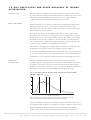
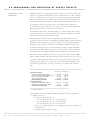
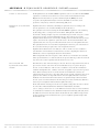
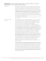
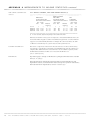
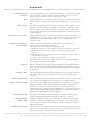
FREQ U EN C Y
A frequency distribution illustrates the location and spread of income within a
DIST R I B U T I O N
population. It groups the population into classes by size of household income and gives
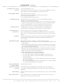
the number or proportion of people in each income range. A graph of the frequency
distribution is a good way to portray the essence of the income distribution. Graph 1.6.1
below shows the proportion of people within $50 household income ranges.
1. 6 . 1 DI S T R I B U T I O N OF EQ U I V A L I S E D DI S P O S A B L E HO U S E H O L D
IN C O M E , 20 0 7 – 0 8
%
8
P10
Median Mean
P90
6
4
2
0
0
200
400
600
800 1000 1200 1400 1600 1800 2000
Income ($ per week)
Note: Persons with an income between $25 and $2,025 are shown in $50 ranges on the graph.
Source: Household Income and Income Distribution, Australia, 2007–08 (6523.0)
Frequency distributions can provide considerable detail about variations in the income of
the population being described, but it is difficult to describe the differences between two
frequency distributions. They are therefore often accompanied by other summary
statistics, such as the mean and median. Taken together, the mean and median can
ABS • INFOR M A T I O N PAP ER : SUR V E Y OF INCOM E AND HOU SI N G , USER GUI D E , AUST R A L I A • 655 3 . 0 • 200 7 – 0 8
13
1.6 GINI COEF F I C I E N T AND OTHER MEASU R E S OF INCO M E
D I S T R I B U T I O N continued
FREQ U EN C Y
provide an indication of the shape of the frequency distribution. As can be seen in the
D I S T R I B U T I O N continued
graph above, the distribution of income tends to be asymmetrical, with a small number
of people having relatively high household incomes and a larger number of people
having relatively lower household incomes. The greater the asymmetry, the greater the
difference between the mean and the median.
QUAN T I L E MEAS U R E S
When persons (or any other units) are ranked from the lowest to the highest on the
basis of some characteristic such as their household income, they can then be divided
into equally sized groups. The generic term for such groups is quantiles.
Quintiles , deciles and
When the population is divided into five equally sized groups, the quantiles are called
percentiles
quintiles. If there are 10 groups, they are deciles, and division into 100 groups gives
percentiles. Thus the first quintile will comprise the first two deciles and the first 20
percentiles.
SIH publications frequently present data classified into income quintiles, supplemented
by data relating to the 2nd and 3rd deciles combined. The latter is included to enable
quintile style analysis to be carried out without undue impact from very low incomes
which may not accurately reflect levels of economic wellbeing. (See section 1.5 'Low
income households').
Equivalised disposable household income is the income measure used to define the
quantiles shown in SIH publications, and the quantiles each comprise the same number
of persons, that is, they are person weighted.
Upper values , medians
In some analyses, the statistic of interest is the boundary between quantiles. This is
and percentile ratios
usually expressed in terms of the upper value of a particular percentile. For example, the
upper value of the first quintile is also the upper value of the 20th percentile and is
described as P20. The upper value of the ninth decile is P90. The median of a whole
population is P50, the median of the 3rd quintile is also P50, the median of the first
quintile is P10, etc.
Percentile ratios
Percentile ratios summarise the relative distance between two points on the income
distribution. To illustrate the full spread of the income distribution, the percentile ratio
needs to refer to points near the extremes of the distribution, for example, the P90/P10
ratio. The P80/P20 ratio better illustrates the magnitude of the range within which the
incomes of the majority of the population fall. The P80/P50 and P50/P20 ratios focus on
comparing the ends of the income distribution with the midpoint (the median).
INCO M E SHAR E S
Income shares can be calculated and compared for each income quintile (or any other
subgrouping) of a population. The aggregate income of the units in each quintile is
divided by the overall aggregate income of the entire population to derive income
shares.
GINI COEF F I C I E N T
The Gini coefficient is a single statistic which summarises the distribution of income
across the population.
14
ABS • INFOR M A T I O N PAP ER : SUR V E Y OF INCOM E AND HOU SI N G , USER GUI D E , AUST R A L I A • 655 3 . 0 • 200 7 – 0 8
1.6 GINI COEF F I C I E N T AND OTHER MEASU R E S OF INCO M E
D I S T R I B U T I O N continued
G I N I C O E F F I C I E N T continued
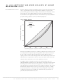
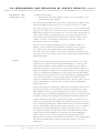
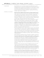
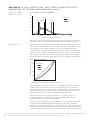
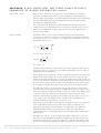
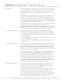
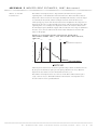
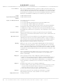
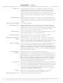
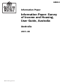
The Gini coefficient can best be described by reference to the Lorenz curve. The Lorenz
curve is a graph with the horizontal axis showing the cumulative proportion of the
persons in the population ranked according to household income and with the vertical
axis showing the corresponding cumulative proportion of equivalised disposable
household income. The graph then shows the income share of any selected cumulative
proportion of the population, as can be seen below in graph 1.6.2.
1. 6 . 2 LO R E N Z CU R V E S
100
Cumulative proportion of income (%)
All persons
Persons in one
parent households
80
60
40
20
0
0
20
40
60
80
100
Cumulative proportion of persons ranked according to income (%)
If income were distributed evenly across the whole population, the Lorenz curve would
be the diagonal line through the origin of the graph. The Gini coefficient is defined as
the ratio of the area between the actual Lorenz curve and the diagonal (or line of
equality) and the total area under the diagonal. The Gini coefficient ranges between zero
when all incomes are equal and one when one unit receives all the income, that is, the
smaller the Gini coefficient the more even the distribution of income.
Normally the degree of inequality is greater for the whole population than for a
subgroup within the population because subpopulations are usually more homogeneous
than full populations. This is illustrated in the graph above, which shows two Lorenz
curves from the 2007–08 SIH. The Lorenz curve for the whole population of the survey is
further from the diagonal than the curve for persons living in one parent, one family
households, with at least one dependent child. Correspondingly, the calculated Gini
coefficient for all persons was 0.331 while the coefficient for the persons in the one
parent households included here was 0.270.
ABS • INFOR M A T I O N PAP ER : SUR V E Y OF INCOM E AND HOU SI N G , USER GUI D E , AUST R A L I A • 655 3 . 0 • 200 7 – 0 8
15
1.6 GINI COEF F I C I E N T AND OTHER MEASU R E S OF INCO M E
D I S T R I B U T I O N continued
G I N I C O E F F I C I E N T continued
The Gini coefficient is discussed in more detail, along with the Theil index and Atkinson
index, in Appendix 3 'Gini coefficient and other single statistic summaries of income
distribution'.
16
ABS • INFOR M A T I O N PAP ER : SUR V E Y OF INCOM E AND HOU SI N G , USER GUI D E , AUST R A L I A • 655 3 . 0 • 200 7 – 0 8
1.7 CHILD CARE
CHIL D CARE
Data on child care including: usage; costs; and barriers to labour force participation due
to child care related reasons, were included in the Survey of Income and Housing (SIH)
for the first time in 2007–08. These topics were added to the SIH due to meet user
requirements and provide data items looking at the interactions between child care use,
income and labour force participation. These data items are not intended to provide a
detailed exploration of child care such as can be found in Childhood Education and
Care, June 2008 (cat. no. 4402.0).
DAT A COLL E C T I O N
Child care information was collected from households containing resident children aged
0–12 years. The information was obtained from an adult who permanently resided in the
household and was deemed to be the 'best person' able to provide this information. In
the majority of cases this was the child's parent, step-parent or guardian.
Questions about type(s) of child care used (formal, informal and other), pattern of care
with other parent living elsewhere, school attendance, preschool attendance and cost of
care were asked in relation to each child aged 0–12 in the household. If formal or
informal care was used by a child in the last four weeks, further questions about cost,
child care benefit and hours used were asked for each episode of care.
DEF I N I T I O N S
Data was collected on child care used in the 4 weeks prior to the personal interview, and
as such most data items relate to 'last 4 weeks'. In addition, data is available for care types
used 'in the last week' where the number of hours of care used last week was one or
more.
Formal and informal child
Formal care is defined as regulated care away from the child's home. The main types of
care
formal care are before and/or after school care, long day care, family day care, occasional
care and vacation care.
Informal care is defined as non-regulated care, arranged by a child's parent/guardian,
either in the child's home or elsewhere. It comprises care by (step) brothers or sisters,
care by grandparents, care by other relatives (including a parent living elsewhere) and
care by other (unrelated) people such as friends, neighbours, nannies or babysitters. It
may be paid or unpaid.
Cost of care
The cost, gross of Child Care Benefit, to parents for a child to attend care. In most cases,
where the Child Care Benefit was paid directly to the child care service provider, the cost
of care was directly collected in the survey. In a small number of cases, where the Child
Care Benefit was not paid directly to the provider, the Child Care Benefit was estimated.
Information on the Child Care Tax Rebate was not included as part of the survey.
Child Care Benefit (CCB)
Assistance in the form of a payment made by the Australian Government to help with the
costs of child care for families who use either approved or registered child care. The CCB
was introduced on 1 July 2000, when it replaced the Childcare Cash Rebate and
Childcare Assistance.
ABS • INFOR M A T I O N PAP ER : SUR V E Y OF INCOM E AND HOU SI N G , USER GUI D E , AUST R A L I A • 655 3 . 0 • 200 7 – 0 8
17
1 . 7 C H I L D C A R E continued
Child Care Tax Rebate
A tax offset, passed by Parliament in December 2005. In general terms, as a result of the
(CCTR)
Child Care Tax Rebate, families with a tax liability will be eligible for 30 percent, as at
June 2008, of out–of–pocket expenses incurred for approved child care, up to a
maximum of $4,354 per child per year. The CCTR applies to out–of–pocket expenses for
approved child care. The CCTR is available for families who receive Child Care Benefit
(CCB) and meet the CCB work, study and training test.
Barriers to labour force
Data on barriers to labour force participation due to child care related reasons was
partic ipation due to child
collected from parents/guardians of children aged 0–12 years old in the selected
care related reasons
household who were unemployed, did not have a job or worked part time. The data
collected includes if people would like a job if child care was available, if they would like
to work more hours if child care was available, if child care prevents them from
working/working more hours, and what are all and the main reason child care prevents
them for working/working more hours. This detail is available at the person level.
USIN G THE DAT A
Units for analys is
The income unit is the preferred level of analysis as other income unit characteristics,
such as income and number of persons etc, can be cross-classified at this level. Like
households, resources at the income unit level is normally shared between partners in a
couple relationship and with dependent children. However, there are limitations on the
data provided at this level. At the income unit level child care data are aggregated from
lower levels and as such may apply to more than one child in an income unit. For
example, in an income unit where more than one child was cared for by a parent living
elsewhere with differing frequencies of care, the item 'Most frequent pattern of care with
child's other parent living elsewhere' relates to the most frequent care pattern used by
one of the children.
More than one type of care could be selected, therefore some items are multi-response
in nature.
18
ABS • INFOR M A T I O N PAP ER : SUR V E Y OF INCOM E AND HOU SI N G , USER GUI D E , AUST R A L I A • 655 3 . 0 • 200 7 – 0 8
1.8 HOUS E H O L D , INCO M E UNIT , PERS O N AND LOAN DATA
HOUSE H O L D, INCO ME
The SIH collects information with respect to households and all the people comprising
UNIT , PER SO N AND LOAN
those households. It is therefore possible to produce aggregate data from the survey to
DAT A
households, to persons, or with respect to combinations of persons within the
household such as income units. Analysts can choose the unit of analysis most suited to
their purposes. The data item list referred to in section 2.3 'Data collection and data item
description' shows which data items are available for each unit type supported by the
SIH.
Households
A household consists of one or more persons, at least one of whom is at least 15 years of
age, usually resident in the same private dwelling. The persons in a household may or
may not be related. They must live wholly within one dwelling. A group of people who
make common provision for food and other essentials of living but live in two separate
dwellings are in two separate households.
Most of the published output from the SIH uses the household as the unit of analysis
and relates to characteristics of the households.
Income units
An income unit is one person or a group of related persons within a household, whose
command over income is assumed to be shared. Income sharing is assumed to take
place within married (registered or de facto) couples, and between parents and
dependent children. The income unit is similar, but not identical, to the unit used in
determining the eligibility of people for many government pensions and allowances such
as Centrelink payments.
Income data and selected income unit characteristics are available on an income unit
basis from the SIH, although they are not included in any published output from the
survey.
Persons
Data at the person level are available for each person aged 15 years and over usually
resident in the households included in the SIH. Data relating to characteristics of
children under the age of 15 are only available at the household level.
Loans
A household may have one or more loans, and data are available for characteristics of
each loan, such as the main purpose, security, amount borrowed, principal outstanding
and weekly repayment, although they are not included in detail in any published output
from the survey.
Units used in SIH
Analysis of income data is usually carried out using household income measures. As
publis hed output
explained in section 1.3 'Equivalised household income', it is normally most appropriate
to examine household income when considering economic wellbeing, because of the
sharing that occurs between members of households. That section also explains that
income comparisons are improved if the household income measure is adjusted to
reflect the size and composition of the household.
However, when analysing income distribution, it is the number of people who belong to
households with particular characteristics, rather than the number of households with
those characteristics, that is of primary interest. This leads to the preference for the
equal representation of those persons in such analysis. For example, if the person is used
as the unit of analysis rather than the household, then the representation in the income
ABS • INFOR M A T I O N PAP ER : SUR V E Y OF INCOM E AND HOU SI N G , USER GUI D E , AUST R A L I A • 655 3 . 0 • 200 7 – 0 8
19
1.8 HOUS E H O L D , INCO M E UNIT , PERS O N AND LOAN DATA
continued
Units used in SIH
distribution of each person in a household comprising four persons is the same as that
publis hed output continued
for each person in a household comprising two persons. In contrast, if the household
were to be used as the unit of analysis, each person in the four person household would
only have half the representation of each person in the two person household.
Therefore, the income distribution measures from the SIH are all calculated with respect
to persons, including children. Such measures are sometimes known as person weighted
estimates because the unit of analysis is the person, even though all the characteristics
being described are characteristics of the household to which the person belongs. The
method of calculation is described in section 2.7 'Calculation of population counts,
means, medians and other estimates'.
20
ABS • INFOR M A T I O N PAP ER : SUR V E Y OF INCOM E AND HOU SI N G , USER GUI D E , AUST R A L I A • 655 3 . 0 • 200 7 – 0 8
1.9 REFE R E N C E PERS O N
REFE R E N C E PER S O N
In some analyses it is useful to describe a household or income unit using characteristics
that are in essence attributes of persons. For example, the analyst may wish to classify
households into 'older households' and 'younger households'. One approach often used
is to designate one member of the household or income unit as the reference person,
and assume that the characteristics of that person are descriptive of the household or
income unit more generally. The reference person is chosen through a set of operating
procedures designed to identify a person most likely to be representative of the
household or income unit. Households or income units can then be classified according
to the age of the reference person, occupation of the reference person, country of birth
of the reference person, etc.
Household reference
The reference person for each household is chosen by applying, to all household
person
members aged 15 years and over, the selection criteria below, in the order listed, until a
single appropriate reference person is identified:
!
the person with the highest tenure when ranked as follows: owner without a
mortgage, owner with a mortgage, renter, other tenure
!
one of the partners in a registered or de facto marriage, with dependent children
!
one of the partners in a registered or de facto marriage, without dependent children
!
a lone parent with dependent children
!
the person with the highest income
!
the eldest person.
For example, in a household containing a lone parent (owner with a mortgage) with a
non–dependent child, the one with the higher tenure will become the reference person.
However, if both individuals have the same tenure (eg a couple, owners with a
mortgage), the one with the highest income will become the reference person.
Income unit referenc e
The reference person for an income unit is the male partner in a couple income unit, the
person
parent in a one parent income unit and the person in a one person income unit.
ABS • INFOR M A T I O N PAP ER : SUR V E Y OF INCOM E AND HOU SI N G , USER GUI D E , AUST R A L I A • 655 3 . 0 • 200 7 – 0 8
21
1.10 HOUSI N G STAT I S T I C S
HOU S I N G UTILISA T IO N
The concept of housing utilisation derived for the SIH is based upon a comparison of the
number of bedrooms in a dwelling with a series of household demographics such as the
number of usual residents, their relationship to one another, age and sex. There is no
single standard of measure for housing utilisation. However the Canadian National
Occupancy Standard (CNOS) derived for the SIH is widely used internationally.
The Canadian National Occupancy Standard for housing appropriateness is sensitive to
both household size and composition. The measure assesses the bedroom requirements
of a household by specifying that:
!
there should be no more than two persons per bedroom
!
children less than 5 years of age of different sexes may reasonably share a bedroom
!
children less than 18 years of age and of the same sex may reasonably share a
bedroom
!
single household members 18 years and over should have a separate bedroom, as
should parents or couples
!
a lone person household may reasonably occupy a bed sitter.
The CNOS variable on the file compares the number of bedrooms required with the
actual number of bedrooms in the dwelling. Households living in dwellings where this
standard cannot be met are considered to be overcrowded.
HOUSI N G COSTS AND
Housing costs are recurrent outlays by household members in providing for their
HOUS I N G STRES S
shelter. The data collected on housing outlays in the SIH are limited to major cash
outlays on housing, that is, mortgage repayments, rent, property and water rates as well
as body corporate fees.
Only payments which relate to the dwelling occupied by the household at time of
interview, that is, a respondent's usual place of residence, are included. Housing costs
only include mortgage/loan payments if the purpose of the loan at the time it was initially
taken out was primarily to buy, build, add to or alter the occupied dwelling.
There are a number of limitations to the housing costs information obtained in the SIH,
due to practical data collection considerations. These limitations should be especially
borne in mind when comparing the housing costs of different tenure and landlord types,
that is, when comparing the costs of owner occupiers with the costs of renting
households, and when comparing the costs of households renting from state and
territory housing authorities with the costs of other renters.
!
Households are sometimes reimbursed some or all of their housing costs.
Commonwealth Rent Assistance (CRA), paid by the Australian Government to
qualifying recipients of income support payments and family tax benefit, is the most
important type of reimbursement of relevance to these statistics. If rent assistance
receipts were subtracted from gross housing costs, it has been estimated that the
housing costs of households receiving rent assistance would be about 30% lower on
average, and the housing costs of all households renting from landlords other than
the state/territory authorities would be about 10% lower on average.
22
ABS • INFOR M A T I O N PAP ER : SUR V E Y OF INCOM E AND HOU SI N G , USER GUI D E , AUST R A L I A • 655 3 . 0 • 200 7 – 0 8
1 . 1 0 H O U S I N G S T A T I S T I C S continued
HOUSI N G COSTS AND
!
H O U S I N G S T R E S S continued
Mortgage repayments made by owners with a mortgage include both the interest
component and the principal or capital component. For many purposes it is more
appropriate to consider repayments of principal as a form of saving rather than as a
recurrent housing cost. It reflects the purchase of a housing asset by increasing the
equity in the property held by the household and is an addition to the wealth of the
occupants. The 2007–08 SIH indicated that about 32% of the housing costs of
owners with a mortgage comprised repayments of the principal on loans. The
equivalent proportions in 2005–06 and 2003–04 were 36% and 40% respectively.
!
A fuller measure of housing costs would include a range of outlays not collected in
the SIH, but which are necessary to ensure that the dwelling can continue to
provide an appropriate level of housing services. These include repairs,
maintenance, and dwelling insurance, and are costs that tend to be incurred by
owner occupier households but not by renting households. Previous HES data
shows that if these costs were added to SIH housing costs estimates, the estimates
of average housing costs would be more than doubled for owners without a
mortgage and would increase by about 15% for owners with a mortgage.
Housing costs and
Housing costs can be a major component of total living costs. Therefore housing costs
household income
are often analysed as a proportion of total income, sometimes referred to as affordability
ratios. However, comparisons between these measures are subject to the limitations of
housing cost estimates obtained in the SIH that are described in the previous paragraph.
Housing affordability ratios derived from SIH data are further impacted by the inclusion
of CRA in the value of income collected. In earlier research CRA has been estimated, on
average, to represent about 8% of the reported income of households receiving CRA and
about 2% of the reported income of all households renting from landlords other than
the state/territory authorities.
To illustrate the difficulties discussed above, consider two households that are renting
their dwellings. Both receive government pensions of $400 per week. One rents from a
public housing authority and pays rent of $100 per week. The other pays $135 rent per
week to a private landlord and receives Commonwealth Rent Assistance of $35. In SIH,
the housing costs of the latter household would be recorded as $135 and their income
would be recorded as $435. The couple renting from the public housing authority has a
housing costs/income ratio of 25%. The housing costs/income ratio for the latter
household would be derived as 31%. If CRA receipts are excluded from housing costs
and income the housing costs/income ratio for the latter couple is also 25%, highlighting
that there is no substantive difference between the housing costs or income situation of
the two couples. This anomaly is of particular concern when considering changes in
affordability ratios over time, since there has been a shift from providing public housing
to providing CRA as a means of supplying affordable housing to low income people.
While housing costs can be a major component of total living costs, the difference
between the housing costs of a larger household and a smaller household would not be
expected to be as great as the difference in many other costs, such as food or clothing. In
other words, larger households can be expected to experience economies of scale in the
supply of housing. This means that if a larger household and smaller household both
have the same standard of living, it could be expected that on average the larger
household will have a lower housing costs/income ratio. Therefore relatively high
ABS • INFOR M A T I O N PAP ER : SUR V E Y OF INCOM E AND HOU SI N G , USER GUI D E , AUST R A L I A • 655 3 . 0 • 200 7 – 0 8
23
1 . 1 0 H O U S I N G S T A T I S T I C S continued
Housing costs and
housing costs/income ratios are more of a concern with respect to larger households
household income
than smaller households. This should be borne in mind when comparing ratios across
continued
different household sizes.
In comparing households' housing costs with their income, it should be noted that
households have a variety of housing preferences. Some people may choose to live in an
area with high land values because it is close to their place of employment and therefore
they have lower transport costs. Some people choose to incur relatively high housing
costs because they prefer a relatively high standard of housing instead of other
consumption possibilities. High mortgage repayments might reflect a choice to purchase
a relatively expensive home, or pay off a mortgage relatively rapidly, as a form of
investment.
Housing stres s
Households with relatively low income and housing costs greater than a certain
proportion of income, often 30%, are sometimes said to be in 'housing stress'. The ABS
does not use that term in its published output from SIH to label households meeting
those criteria because of the lack of comparability of the housing affordability ratios
across tenure and landlord types, and the difficulties of comparing across different
household sizes, as described in the previous paragraphs.
ADDI T I O N A L HOU S I N G
The SIH 2007–08 included additional housing topics to enable reporting on the broader
CONT E N T COLLE C T E D IN
housing circumstances of non-Indigenous Australians. The ABS will collect additional
2007 – 0 8
information on housing in the SIH every six years. For 2007–08, housing topics include:
housing mobility, housing condition and dwelling characteristics, home purchase for first
home buyers, household finances of owners with a mortgage, rental arrangements and
the affairs of renters, and neighbourhood.
Refer to Appendix 6 'Additional Housing Topics', for more information on additional
housing data.
24
ABS • INFOR M A T I O N PAP ER : SUR V E Y OF INCOM E AND HOU SI N G , USER GUI D E , AUST R A L I A • 655 3 . 0 • 200 7 – 0 8
PART 2 SURV E Y METH O D O L O G Y
SUR V E Y MET H O D O L O G Y
Part 2 of this User Guide describes the methodology used for the 2007–08 Survey of
Income and Housing (SIH), including:
!
information about the scope, coverage and sample
!
data collection and processing
!
benchmarks and weighting
!
estimates and reliability of estimates.
Changes to survey methodology in 2007–08 are described in Part 4 'Changes from
previous surveys'.
ABS • INFOR M A T I O N PAP ER : SUR V E Y OF INCOM E AND HOU SI N G , USER GUI D E , AUST R A L I A • 655 3 . 0 • 200 7 – 0 8
25
2.1 SCOPE AND COVER A G E
SCO P E
The survey collects information by personal interview from usual residents of private
dwellings in urban and rural areas of Australia (excluding very remote areas), covering
about 97% of the people living in Australia. Private dwellings are houses, flats, home
units, caravans, garages, tents and other structures that were used as places of residence
at the time of interview. Long-stay caravan parks are also included. These are distinct
from non-private dwellings which include hotels, boarding schools, boarding houses and
institutions. Residents of non-private dwellings are excluded.
Usual residents excludes:
!
households which contain members of non-Australian defence forces stationed in
Australia, and
!
households which contain diplomatic personnel of overseas governments.
For most states and territories the exclusion of people in very remote areas has only a
minor impact on any aggregate estimates that are produced because they only constitute
a small proportion of the population. Very remote and remote areas are defined by the
assignment of an Accessibility/Remoteness Index of Australia (ARIA) score. ARIA is a
remoteness value (a continuous variable between 0 and 15) that measures the physical
distance which separates people in a particular area and where their goods, services and
opportunities for social interaction may be accessed. The range of ARIA scores have been
categorised as follows:
!
Least Remote: Defined as having an ARIA score less then 5.95.
!
Remote: Defined as having an ARIA score greater than or equal to 5.95 but less than
10.5.
!
Very Remote: Defined as having an ARIA score greater than or equal to 10.5.
The ARIA categories and how ARIA scores are calculated are further explained in the
Australian Standard Geographical Classification (ASGC) (cat. no. 1216.0).
COVE R AGE
Information was collected only from usual residents. Usual residents were residents who
regarded the dwelling as their own or main home. Others present were considered to be
visitors and were not asked to participate in the survey.
26
ABS • INFOR M A T I O N PAP ER : SUR V E Y OF INCOM E AND HOU SI N G , USER GUI D E , AUST R A L I A • 655 3 . 0 • 200 7 – 0 8
2.2 SELEC T E D SAMPL E AND FINA L SAMPL E
SAMP L E DESI G N
The sample was designed to produce reliable estimates for broad aggregates for
households resident in private dwellings aggregated for Australia, for each state and for
the capital cities in each state and territory. More detailed estimates should be used with
caution, especially for Tasmania, the Northern Territory and the Australian Capital
Territory (see Section 2.8 'Reliability of estimates').
In the 2007–08 SIH, dwellings were selected through a stratified, multistage cluster
design. Selections were distributed across a eleven month enumeration period. The SIH
is normally conducted over a 12 month enumeration period so that the survey results
would be representative of income patterns across the year. In 2007–08 the estimates
were adjusted during weighting so that the shorter enumeration period in the first
quarter was compensated in the final estimates. In the final quarter of enumeration, 10%
of the selected dwellings were deselected from the sample. This reduced the overall
number of dwellings selected to participate in the survey. This outcome may increase the
standard error in the final quarter estimates and hence the standard error in the
annualised estimates. The relative change in sample size across the enumeration quarters
may also introduce some bias to the annualised estimates but this is expected to be
much less than the standard error.
SELE C T E D DWEL L I N G S ,
In the 2007–08 SIH, 11,126 dwellings were selected for the sample. This excludes
SAMP L E LOSS AND
dwellings removed as part of the deselection mentioned above. When field work
SELE C T E D HOU S E H O L D S
commenced some dwellings selected for inclusion in the SIH sample were found to have
no possibility of delivering a survey response. Collectively these are referred to as sample
loss, and are composed of the following groups:
!
dwellings which are out of scope of the survey; under construction, demolished, or
converted to non-private dwellings or non-dwellings
!
vacant private dwellings
!
private dwellings that only contain only either out of scope residents (e.g. dwelling
occupied by foreign diplomats and their dependents) or visitors.
In 2007–08 sample loss and non-response was 1,781 dwellings, 16% of the selected
sample.
Sometimes dwellings that have been selected for inclusion in a survey are found to
comprise more than one actual dwelling because, for example, an additional residence
such as a 'granny flat' has been added to the original dwelling. In such cases, each actual
dwelling becomes a separate household. Occasionally the residents of a selected
dwelling request that their details be provided separately from other dwelling residents,
for privacy reasons. A separate household is created for each such group of residents. In
2007–08, 33 selected dwellings were split into 2 households, 2 were split into 3, and 1
was split into 4.
RESPO N DI N G
Households selected for inclusion in the survey can be categorised as responding or
HOUSE H O L DS AND FINAL
non-responding households. Responding households are either fully responding or
SAMP L E
partially responding. In the SIH, information missing from partially responding
households is imputed, as described in 2.4 'Data processing'.
Non-responding households include:
!
households affected by death or illness of a household member
ABS • INFOR M A T I O N PAP ER : SUR V E Y OF INCOM E AND HOU SI N G , USER GUI D E , AUST R A L I A • 655 3 . 0 • 200 7 – 0 8
27
2 . 2 S E L E C T E D S A M P L E A N D F I N A L S A M P L E continued
RESPO N DI N G
!
HOUSE H O L DS AND FINAL
households in which the significant person(s) in the household did not respond
because they could not be contacted, had language problems or refused to
S A M P L E continued
participate
!
households in which the significant person(s) did not respond to key questions.
The final sample on which estimates were based, is composed of persons for which all
necessary information is available. The information may have been wholly provided at
the interview (fully-responding) or may have been completed through imputation for
partially responding households. Of the selected dwellings, there were 11,126 in the
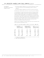
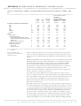
scope of the survey, of which 9,345 (84.0%) were included as part of the final estimates.
The final sample consists of those 9,345 households, comprising 18,326 persons aged 15
years old and over. The final sample includes 2,026 households which had at least one
imputed value in income or child care expenses. For 52.4% of these households only a
single value was missing, and most of these were for income from interest and
investments or information relating to household loans.
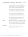
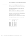
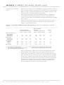
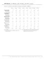
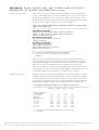
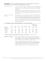
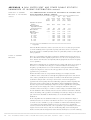
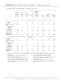
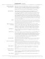
Table 2.2.1 shows the distribution of the final samples between states and territories and
between capital cities and the balance of state.
TA B L E 2. 2 . 1 SI H FI N A L SA M P L E , Nu m b e r of ho u s e h o l d s — 20 0 7 – 08
CAPITAL CITY
TOTAL
Households
Persons(a)
Households
Persons(a)
Households
Persons(a)
no.
no.
no.
no.
no.
no.
NSW
Vic.
Qld
SA
WA
Tas.
NT
ACT
1 193
1 309
749
1 063
965
283
268
428
2 423
2 633
1 559
2 016
1 896
538
538
869
765
482
828
292
269
387
64
—
1 433
936
1 588
544
513
712
128
—
1 958
1 791
1 577
1 355
1 234
670
332
428
3 856
3 569
3 147
2 560
2 409
1 250
666
869
Aust.
6 258
12 472
3 087
5 854
9 345
18 326
—
(a)
28
BALANCE OF STATE
nil or rounded to zero (including null cells)
Number of persons aged 15 years and over
ABS • INFOR M A T I O N PAP ER : SUR V E Y OF INCOM E AND HOU SI N G , USER GUI D E , AUST R A L I A • 655 3 . 0 • 200 7 – 0 8
2.3 DATA COLLE C T I O N AND DATA ITEM DESCR I P T I O N
INT E R V I E W PRO C E D U R E S
Experienced ABS interviewers were used to collect SIH data. They were given
comprehensive training and were provided with detailed written instructions to
complement the survey documents.
Information for each household was collected using:
!
a household level computer assisted interview questionnaire which collected
information on household characteristics, housing costs and certain assets and
liabilities
!
an individual level computer assisted interview questionnaire which collected
information on income and personal characteristics from each usual resident aged
15 years and over in all households.
Interviewers made an initial contact visit, in which they obtained information on the
numbers and characteristics of people usually resident in the dwelling. If a responsible
adult was not available, the interviewer called back at another time. The interviewer also
arranged a convenient time to call back to conduct the interviews.
During the actual survey interview, the interviewer:
!
completed one household questionnaire for each household (information was
provided by a household spokesperson who was nominated as the best person to
provide information on the financial situation of the household)
!
completed an individual questionnaire for each usual resident aged 15 years and
over.
If a usual resident could not be present for the interview, additional interviews were
arranged to ensure that all usual residents were covered by the survey.
DAT A COLL E C T I O N
A representation of the computer assisted interview questionnaires used in the SIH can
INST R U ME N T S
be downloaded as separate pdf files from the "Downloads" tab of the website entry for
this publication.
DATA ITEM S AVAI L A B L E
A listing of all the data items available from the SIH can be downloaded from the
"Downloads" tab of the website entry for this publication.
ABS • INFOR M A T I O N PAP ER : SUR V E Y OF INCOM E AND HOU SI N G , USER GUI D E , AUST R A L I A • 655 3 . 0 • 200 7 – 0 8
29
2.4 DATA PROC E S S I N G
DAT A PRO C E S S I N G
Computer based systems were used to process the data from the SIH with a program
MET H O D S
known as BLAISE. It was necessary to employ a variety of methods to process and edit
the data which reflected the different questionnaires used to collect data from the
household and individual components of the surveys. These processes are outlined
below.
Coding and input editing
Internal system edits were applied in the computer-assisted interview (CAI)
of hous ehold and
questionnaires to ensure the completeness and consistency of the responses being
indiv idual questionnaires
provided. The interviewer could not proceed from one section of the interview to the
next until responses had been appropriately completed.
A number of range and consistency edits were programmed into the CAI questionnaire.
Edit messages automatically appeared on the screen if the information entered was
either outside the permitted range for a particular question, or contradicted information
already recorded. These edit queries were resolved on the spot with respondents.
Data from the CAI questionnaires were electronically loaded to the processing database
on receipt in the ABS office in each State or Territory. There, checks were made to
ensure data for all relevant questions were fully accounted for and that returns for each
household and respondent were obtained. Problems identified by interviewers were
resolved by office staff, where possible, based on other information contained in the
schedule, or on the comments provided by interviewers.
Computer-assisted coding was performed on responses to questions on country of birth,
occupation and industry of employment to ensure completeness. Data on relationships
between household members were used to delineate families and income units within
the household, and to classify households and income units by type.
A query resolution system ensured that an accurate record of decisions was made in
resolving the queries.
Additional editing
A range of edits was also applied to the household and individual information to double
check that logical sequences had been followed in the questionnaires; that specific
values lay within expected ranges; and that relationships between items were consistent.
Unusually high values (termed statistical outliers) were investigated to determine
whether there had been errors in entering the data. Such values were also examined for
their effect on aggregate estimates for Australia, and action was taken where necessary.
Imputation for missing
Some other households did not supply all the required information but supplied
records and values
sufficient information to be retained in the sample. Such partial response occurs when:
!
income or other data in a questionnaire are missing from one or more
non-significant person's records because they are unable or unwilling to provide the
data
!
all key questions are answered by the significant person(s) but other data are
missing.
In these cases, the data provided are retained and the missing data are imputed by
replacing each missing value with a value reported by another person (referred to as the
donor).
30
ABS • INFOR M A T I O N PAP ER : SUR V E Y OF INCOM E AND HOU SI N G , USER GUI D E , AUST R A L I A • 655 3 . 0 • 200 7 – 0 8
2 . 4 D A T A P R O C E S S I N G continued
Imputation for missing
Donor records are selected by finding fully responding persons with matching
records and values
information on various characteristics (such as state, sex, age, labour force status and
continued
income) as the person with missing information. As far as possible, the imputed
information is an appropriate proxy for the information that is missing. Depending on
which values are to be imputed, donors are randomly chosen from the pool of individual
records with complete information for the block of questions where the missing
information occurs.
In the 2007–08 SIH, responses were imputed when not every person aged 15 or over
residing in the household responded, but the significant persons provided answers to all
key questions.
ABS • INFOR M A T I O N PAP ER : SUR V E Y OF INCOM E AND HOU SI N G , USER GUI D E , AUST R A L I A • 655 3 . 0 • 200 7 – 0 8
31
2.5 INCO M E TAX AND OTHER MODEL L E D DATA ITEMS
MODE L L E D DAT A ITEM S
Some data items of interest cannot reliably be collected from respondents, and some
cannot be collected at all. However, in some cases it is possible to utilise other
information provided by respondents as a basis for estimating the data items of interest.
The process is referred to as modelling.
Income tax and the
As described in Section 1.1, disposable income is calculated by deducting income tax
Medic are levy
(including the Medicare levy and surcharge) from gross income. The model is based on
the liability rules described in the Tax Pack for the year concerned, the income reported
by respondents, and other characteristics of household members reported in the survey.
Estimates of income tax are modelled, rather than collected from respondents, for a
number of reasons.
!
As noted in Section 1.4, an accruals approach is taken to estimating these items. The
estimates should therefore relate to the tax liability being incurred with respect to
the income being reported by the respondent in the survey. For estimates of current
income (see Section 1.2 'Current, annual and weekly income'), the current income
tax liability is calculated as though the current income is the average income for the
whole year. If actual income fluctuates during the year, respondents are unlikely to
have an actual income tax assessment that is relevant to the required estimate.
!
In addition to income changes during the course of the year, full year income tax
assessments may be affected by changes in family or other circumstances of the
respondent which are not described in the survey, and are best ignored when
deriving an income tax estimate to use with the other survey data.
!
Income tax assessments are only made after the end of the financial year, and
therefore are not yet available at the time that current income is collected from
respondents.
!
The income tax assessment of respondents may be affected by certain expenditures
which they make, such as donations to charities, or other particular circumstances
which are not captured in the survey. For many purposes it is desirable to exclude
the impact on tax liabilities of specific influences which are not captured in the
survey.
!
The SIH provides sufficient relevant information to allow a relatively comprehensive
model to be constructed.
In 2007–08, the Medicare Levy Surcharge was also modelled and deducted from gross
income while calculating disposable income.
Family tax benefit
Family tax benefit (FTB) can be received as a fortnightly payment from the Family
Assistance Office, a reduction in pay-as-you-go (PAYG) income tax deductions, a lump
sum after the end of the year, or a combination of these. Payments received as
fortnightly payments are collected in the SIH and are used in the derivation of "Current
weekly income from family tax benefits". Benefits received in the form of reduced PAYG
tax or as a lump sum are modelled using responses to the FTB questions relating to
method of payment, as well as other demographic and income information. From
2005–06 income from FTB supplements has also been modelled.
32
ABS • INFOR M A T I O N PAP ER : SUR V E Y OF INCOM E AND HOU SI N G , USER GUI D E , AUST R A L I A • 655 3 . 0 • 200 7 – 0 8
2 . 5 I N C O M E T A X A N D O T H E R M O D E L L E D D A T A I T E M S continued
Family tax benefit
From 2005–06 these modelled components are included in estimates of FTB, and hence
continued
in government pension and allowances, and in gross income. Prior to 2005–06 these
modelled components were treated as negative adjustments in the modelling of income
tax and therefore, while not included in gross income, they were included in disposable
income and equivalised disposable income.
Maternity payment
The 2007–08 SIH collected information on maternity payment received in the previous
financial year, but 'current' estimates of maternity payments could not be collected in the
same way as other pensions and allowances, so the estimates of current income from
maternity payments were modelled. They were treated as though they were paid evenly
through the year, so the payment allocated to eligible recipients was the amount of the
payment divided by 52.14. The payment was assigned to each family with a child aged
under 1 year old at the time of interview. The family was assigned a payment for each
eligible child.
Utilities allowance and
'Current income' estimates of utility allowance and senior concession allowance were
Seniors conces sion
modelled in 2007–08, but were assumed to be included by the respondents in reported
allowance
pension amounts for the previous financial year. These allowances are paid six monthly,
but the amount included in current weekly income is the total payment for the year
divided by 52.14.
Utilities allowance was assigned to all recipients of age pension, wife pension, carer
payment, widow allowance, disability support pension, partner allowance, parenting
payment, austudy, service pension, war widow's pension and special benefit, providing
they were at least 65 years old if male and at least 63 years old if female.
Seniors concession allowance was assigned to males aged 65 and over and females aged
63 and over who are not eligible for the utilities allowance, providing their income unit
income (as reported in the survey) was less than $80,000 per year.
One-off payments to
As described under Government pensions and allowances in Section 1.4 'Components of
carers and older
income', the one-off payments to carers and older Australians were treated as income as
Australians
they were primarily a supplement to existing income support payments.
The one-off payments to carers and to older Australians paid in 2007–08 were modelled
and included in the current estimates of gross income. Similar one-off payments in
2006–07 were assumed to be included by the respondents in reported pension amounts
for previous financial year. These payments are paid once in the year, but the amounts
were modelled as weekly payments through the year.
In the model, the payments are assigned to all respondents expected to have met the
eligibility criteria at the time they were interviewed. The one-off payment to carers was
assigned to recipients of carer payment and carer allowance. The one off payment to
older Australians was assigned to recipients of utilities allowance and seniors concession
allowance.
Child Disability Assistance Payment paid to recipients of carer allowance in 2007 is also
included as part of income in the 2007–08 estimates, recognising that the intention of
the payment is to offset the extra costs of caring for children. The payment was modelled
as paid through out the year.
ABS • INFOR M A T I O N PAP ER : SUR V E Y OF INCOM E AND HOU SI N G , USER GUI D E , AUST R A L I A • 655 3 . 0 • 200 7 – 0 8
33
2.6 BENCH M A R K S AND WEIGH T I N G OF SURVE Y RESUL T S
BENC H M A R K S AND
Weighting is the process of adjusting results from a sample survey to infer results for the
WEIG H T I N G
total in scope population whether that be persons or households. To do this, a 'weight' is
allocated to each sample unit e.g. a person or a household. The weight is a value which
indicates how many population units are represented by the sample unit. The first step
in calculating weights for each unit is to assign an initial weight, which is the inverse of
the probability of being selected in the survey. For example, if the probability of a
household being selected in the survey was 1 in 600, then the household would have an
initial weight of 600 (that is, it represents 600 households).
An adjustment is then made to the initial weights to account for changes in the sample
across the four quarters of survey enumeration; the sum of the weights after this initial
adjustment of households in each quarter is equal.
The initial weights are then calibrated to align with independent estimates of the
population of interest, referred to as 'benchmarks'. Weights calibrated against population
benchmarks ensure that the survey estimates conform to the independently estimated
distribution of the population rather than to the distribution within the sample itself.
In the 2007–08 SIH, all persons in each household were assigned a weight. This differs
from the 2005–06 where children aged 0–14 years were not given separate weights, but
household counts of the number of children were benchmarked to population totals.
The SIH survey was benchmarked to the in scope estimated resident population (ERP)
and the estimated number of households in the population. The 2007–08 cycle has used
population and household benchmarks based on the 2006 Census instead of the 2001
Population Census estimates used for the 2003–04 and 2005–06 SIH. The differences in
the estimated population that occur due to this change are outlined in the following
table.
Population benchmark
Australian Population Benchmark(a)
Persons in Non Private Dwellings Excluded
Persons in Very Remote Excluded
Total Population Exclusions
Final Population Benchmark
Household benchmark
Australian Household Benchmark(a)
Households in Very Remote Excluded
Final Household Benchmark
(a)
2001 Census
2006 Census
21 074 415
392 257
173 102
565 359
20 509 056
21 178 235
371 636
163 470
535 106
20 643 129
8 247 769
61 690
8 186 079
8 136 593
61 348
8 075 244
at 31 December 2007
The benchmarks used in the calibration of the final weights for the 2007–08 SIH were:
!
number of persons —
!
!
by state or territory by age by sex;
●
five year age groups up to 80+ years for the states
●
five year age groups up to 75+ years for the ACT
●
five year age groups up to 60+ years for the NT
by state or the ACT by labour force status ('Employed', 'Unemployed' and 'Not in
the labour force');
!
34
by state by capital city/balance of state;
ABS • INFOR M A T I O N PAP ER : SUR V E Y OF INCOM E AND HOU SI N G , USER GUI D E , AUST R A L I A • 655 3 . 0 • 200 7 – 0 8
2 . 6 B E N C H M A R K S A N D W E I G H T I N G O F S U R V E Y R E S U L T S continued
BENC H M A R K S AND
W E I G H T I N G continued
!
numbers of households —
!
by household composition (number of adults (1,2 or 3+) and whether or not
the household contains children)
More detailed age groupings have been used where possible in 2007–08 SIH. Previously
in the 2003–04 SIH, ten year age groups up to 65 years and over were used . In SIH
2005–06 five year age groups were used up to 75 years and over, except for NT where the
age groups were 15–24, 25–44, 45 and over. The 2007–08 age groups have been refined
further where possible, five year age groups up to 80 years or older in all states. The two
territories have used five year age groups age up to 75 or older for the ACT and 60 or
older for the NT. The expanded detail for age groups in SIH 2007–08 aims to improve
estimates across those ages. The impact of this change on all other estimates not
involving age is expected to be minimal.
The person and household benchmarks were based on preliminary estimates of
numbers of persons and households in Australia (excluding very remote areas) in
2007–08 based on the 2006 Population Census. The benchmarks used include
households and persons residing in occupied private dwellings only and therefore do
not, and are not intended to, match estimates of the total Australian resident population
published by the ABS.
Estimation
Estimates produced from the survey are usually in the form of averages (e.g. average
weekly income of couple households with dependent children), or counts (e.g. total
number of households that own their dwelling or total number of persons living in
households that own their own dwelling). For counts of households, the estimate was
obtained by summing the weights for the responding households in the required group
(e.g. those owning their own dwelling). For counts of persons, the household weights
were multiplied by the number of persons in the household before summing. The SIH
collects data on the number of people, including children, in each household but
separate records with income and other detailed data were only collected for people 15
years and older. Therefore, counts of persons cannot be obtained by summing the
weights of all persons.
Average income values are obtained in two different ways, depending on whether mean
gross household income or mean equivalised disposable household income is being
derived. Estimates of mean gross household income are calculated on a household
weighted basis. They are obtained by multiplying the gross income of each household by
the weight of the household, summing across all households and then dividing by the
estimated number of households. For example, the mean gross household income of
couple households with dependent children is the weighted sum of the gross income of
each such household divided by the estimated number of those households. Estimates
of mean equivalised disposable household income are calculated on a person weighted
basis. They are obtained by multiplying the equivalised disposable income of each
household by the number of people in the household (including children) and by the
weight of the household, summing across all households and then dividing by the
estimated number of people in the population group. Appendix 3 illustrates the
differences between mean gross household income calculated on a household weighted
basis and mean equivalised disposable household income calculated on a person
weighted basis.
ABS • INFOR M A T I O N PAP ER : SUR V E Y OF INCOM E AND HOU SI N G , USER GUI D E , AUST R A L I A • 655 3 . 0 • 200 7 – 0 8
35
2.7 CALC U L A T I O N OF POPU L A T I O N COUN T S , MEAN S , MEDI A N S
AND OTHER ESTIM A T E S
COUN T S
Counts of income units or households are derived by summing the weights assigned to
each income unit or household record of interest. Counts of persons can also be
obtained this way if only persons over 15 years of age are required. However, there are
not separate records for persons under the age of 15, and therefore counts of persons
including those under 15 years have to be derived by first multiplying each household
weight by the number of persons in the household and then summing the products.
MEAN S
The mean, or average, value of a data item is usually calculated by selecting all the survey
records for the population of interest, multiplying the value of the data item in each
record by the weight of the record and summing the resultant products, and then
dividing the total by the sum of the weights of the records. For example, the mean gross
income of Queensland households is the weighted sum of the gross income of each
such household divided by the sum of the weights relating to each such household.
However, for some purposes means for a household variable may be required with
respect to all people in a population group, including children aged under 15. Such
measures (referred to as person weighted measures) are often used when analysing
equivalised household income. Estimates of mean equivalised disposable household
income in SIH published output are obtained by multiplying the equivalised disposable
income of each household by the number of people in the household (including
children) and by the weight of the household, summing across all households and then
dividing by the estimated number of people in the population group. (The estimated
number of people in the population group is calculated as outlined above in the section
'counts', by first multiplying each household weight by the number of persons in the
household and then summing the products).
MEDI A N S
Medians divide the population of interest into halves. To identify the median record, the
population is first ranked in ascending order according to the data item of interest.
Except for person weighted measures of household variables, the weights of the records
are then accumulated until half the population is accounted for. The record at which this
occurs is the median record, and its value for the data item of interest is the median
value. For person weighted measures of household variables, the household weights are
multiplied by the number of persons in the household before accumulation.
OTHE R ESTIMAT E S
An analagous approach is used for other quantile measures.
Calculation of the Gini coefficient is included in Appendix 3 'Gini coefficient and other
single statistic summaries of income distribution'.
36
ABS • INFOR M A T I O N PAP ER : SUR V E Y OF INCOM E AND HOU SI N G , USER GUI D E , AUST R A L I A • 655 3 . 0 • 200 7 – 0 8
2.8 RELIA B I L I T Y OF ESTIM A T E S
RELIABIL ITY OF
The estimates provided in the SIH are subject to two types of error, non-sampling and
ESTI M A T E S
sampling error.
Non-s ampling error
Non-sampling error can occur in any collection, whether the estimates are derived from
a sample or from a complete collection such as a census. Sources of non-sampling error
include non-response, errors in reporting by respondents or recording of answers by
interviewers and errors in coding and processing the data.
Non-sampling errors are difficult to quantify in any collection. However, every effort is
made to reduce non-sampling error to a minimum by careful design and testing of the
questionnaire, training of interviewers and data entry staff and extensive editing and
quality control procedures at all stages of data processing.
One of the main sources of non-sampling error is non-response by persons selected in
the survey. Non-response occurs when people cannot or will not cooperate or cannot be
contacted. Non-response can affect the reliability of results and can introduce a bias. The
magnitude of any bias depends upon the level of non-response and the extent of the
difference between the characteristics of those people who responded to the survey and
those who did not.
The following methods were adopted to reduce the level and impact of non-response:
!
face-to-face interviews with respondents
!
the use of interviewers who could speak languages other than English, where
necessary
!
follow-up of respondents if there was initially no response
!
imputation of missing values
!
ensuring that the weighted data is representative of the population (in terms of
demographic characteristics) by aligning the estimates with population benchmarks.
Sampling error
The estimates are based on a sample of possible observations and are subject to
sampling variability. The estimates may therefore differ from the figures that would have
been produced if information had been collected for all households. A measure of the
sampling error for a given estimate is provided by the standard error, which may be
expressed as a percentage of the estimate (relative standard error).
The estimates in the SIH are based on information obtained from the occupants of a
sample of dwellings. Therefore, the estimates are subject to sampling variability and may
differ from the figures that would have been produced if information had been collected
for all dwellings.
One measure of the likely difference is given by the standard error (SE), which indicates
the extent to which an estimate might have varied because only a sample of dwellings
was included. There are about two chances in three that the sample estimate will differ
by less than one SE from the figure that would have been obtained if all dwellings had
been included, and about 19 chances in 20 that the difference will be less than two SEs.
Another measure of the likely difference is the relative standard error (RSE), which is
obtained by expressing the SE as a percentage of the estimate.
ABS • INFOR M A T I O N PAP ER : SUR V E Y OF INCOM E AND HOU SI N G , USER GUI D E , AUST R A L I A • 655 3 . 0 • 200 7 – 0 8
37
2 . 8 R E L I A B I L I T Y O F E S T I M A T E S continued
Sampling error continued
For estimates of population sizes, the size of the SE generally increases with the level of
the estimate, so that the larger the estimate the larger the SE. However, the larger the
sampling estimate the smaller the SE in percentage terms (RSE). Thus, larger sample
estimates will be relatively more reliable than smaller estimates.
In the survey only estimates with RSEs of 25% or less are considered reliable for most
purposes. Estimates with RSEs greater than 25% but less than or equal to 50% are
annotated by an asterisk to indicate they are subject to high SEs and should be used with
caution. Estimates with RSEs of greater than 50%, annotated by a double asterisk, are
considered too unreliable for general use and should only be used to aggregate with
other estimates to provide derived estimates with RSEs of 25% or less.
RSEs for all tables are provided. The RSEs have been derived using the group jackknife
method. If needed, SEs can be calculated using the estimates and RSEs.
COMP A R A T I V E EST I M A T E S
Proportions and percentages, which are formed from the ratio of two estimates, are also
Proportions and
subject to sampling errors. The size of the error depends on the accuracy of both the
percentages
numerator and the denominator. For proportions where the denominator is an estimate
of the number of households in a grouping and the numerator is the number of
households in a sub-group of the denominator group, the formula for the RSE is given
by:
RSE% xy = [RSE%(x)] 2 − [RSE%(y)] 2
Differenc es between
The difference between survey estimates is also subject to sampling variability. An
estimates
approximate SE of the difference between two estimates (x–y) may be calculated by the
formula:
SE(x − y) = [SE(x)] 2 + [SE(y)] 2
This approximation can generally be used whenever the estimates come from different
samples, such as two estimates from different years or two estimates for two
non-intersecting subpopulations in the one year. If the estimates come from two
populations, one of which is a subpopulation of the other, the standard error is likely to
be lower than that derived from this approximation, but there is no straightforward way
of estimating how much lower.
Significance testing
Statistical significance testing can be undertaken to determine whether it is likely that
there is a difference between two estimates from different samples. The standard error
for the difference between two estimates can be calculated using the formula in the
paragraph above. This standard error is used to calculate the following test statistic:
x−y
SE(x−y )
If the value of this test statistic is greater than 1.96 then there are 19 chances in 20 that
there is a real difference in the two populations with respect to that characteristic.
Otherwise, it cannot be stated with confidence that there is a real difference between the
populations.
38
ABS • INFOR M A T I O N PAP ER : SUR V E Y OF INCOM E AND HOU SI N G , USER GUI D E , AUST R A L I A • 655 3 . 0 • 200 7 – 0 8
PART 3 DATA AVAI L A B I L I T Y
DAT A AVAI L A B I L I T Y
Part 3 of this User Guide describes the range of data available from the SIH 2007–08 in
both published and unpublished form. More detailed information can also be obtained
by telephoning the Living Conditions Client Services team on (02) 6252 7457, or by
emailing <[email protected]>.
ABS • INFOR M A T I O N PAP ER : SUR V E Y OF INCOM E AND HOU SI N G , USER GUI D E , AUST R A L I A • 655 3 . 0 • 200 7 – 0 8
39
3.1 PUBLI C A T I O N S
PUBL I C A T I O N S
The publications available from the 2007–08 SIH are listed below. All can be downloaded
free of charge from the ABS website.
Household Income and Income Distribution (cat. no. 6523.0) presents estimates of
income received by households, classified by various characteristics. Also includes
summary measures of the distribution of household income in Australia. Classifications
used to describe households include income quintile, principal source of household
income, family composition, tenure type, and geographic location. For each category of
household, estimates of household size and other characteristics are provided in
addition to the estimates of income.
Housing Occupancy and Costs (cat. no. 4130.0) contains data from the SIH on
Australian housing occupancy and costs, and relates these to characteristics of occupants
and dwellings such as tenure, family composition of household, dwelling structure, age,
income and principal source of income. Also includes value of dwelling estimates and
information on recent home buyers.
Housing Mobility and Conditions (cat. no. 4130.0.55.002) contains data from the SIH on
Australian housing mobility and dwelling conditions. The selected housing topics include
length of time in dwelling, number of times moved in last five years, reasons for moving,
and characteristics of the previous dwelling occupied. They include aspects of the
dwelling occupied, such as any major structural problems, repairs and maintenance
carried out in the past 12 months, and sources of energy and water. For first home
buyers, data on home deposits paid and any monetary assistance received for the
purchase are provided.
Information Paper: Survey of Income and Housing, User Guide, Australia, 2007–08
(cat. no. 6553.0) describes the definitions, concepts, methodology and estimation
procedures used in collecting and processing the data from the SIH. It enables users to
make informed choices on the suitability of the estimates for particular uses. It also
provides a list of all data items available from the survey and a copy of the survey
questionnaire.
Survey of Income and Housing - Confidentialised Unit Record File, Technical Manual,
2007–08 (cat. no. 6541.0) contains details of the confidentialised unit record file (CURF),
including a list of all data items on the file, and background information about the
survey.
The earlier publications on experimental estimates relating to the SIH are listed below.
All can be downloaded free of charge from the ABS website.
Experimental Estimates of Imputed Rent, Australia, 2003–04 and 2005–06 (cat. no.
6525.0) This Information Paper presents household level estimates of the imputed rent
for owner-occupied dwellings derived from the 2003–04 and 2005–06 Surveys of Income
and Housing and the 2003–04 Household Expenditure Survey.
Estimates of Personal Income for Small Areas, 2001–02 to 2005–06 (cat. no.
6524.0.55.002) These data cubes contain estimates of the sources of personal income
people received for each year from 2001–02 to 2005–06. Each of the tables provide a
breakdown of total personal income by the following sources - wage & salary, own
unincorporated business, investment, superannuation and annuity, and other income.
40
ABS • INFOR M A T I O N PAP ER : SUR V E Y OF INCOM E AND HOU SI N G , USER GUI D E , AUST R A L I A • 655 3 . 0 • 200 7 – 0 8
3.2 SPECI A L DATA SERV I C E S
SPEC I A L DAT A SER VI C E S
The published data are only a small portion of the data collected in the survey. The ABS
offers specialised consultancy services to assist clients with more complex statistical
information needs. Clients may wish to have the unit record data analysed according to
their own needs, or require tailored tables incorporating data items and populations as
requested by them. A wide range of data items are available — the detailed list of
possible data items is contained in Appendix 7 'Data item listing'.
Tables and other analytic outputs can be made available electronically or in printed form.
However, as the level of detail or disaggregation increases with detailed requests, the
number of contributors to data cells decreases. This may result in some requested
information not being able to be released due to confidentiality or sampling variability
constraints. All specialist consultancy services attract a service charge, and clients will be
provided with a quote before information is supplied. For further information, contact
ABS information consultants on 1300 135 070 (international callers +61 2 9268 4909).
For clients with specific requirements, customised tables can be produced.
ABS • INFOR M A T I O N PAP ER : SUR V E Y OF INCOM E AND HOU SI N G , USER GUI D E , AUST R A L I A • 655 3 . 0 • 200 7 – 0 8
41
3.3 SUPPO R T I N G MATER I A L
SUPP O R T I N G MAT E R I A L
To assist clients in analysing the data from the survey, a representation of the computer
assisted interview questionnaire used in the SIH is available on the ABS website. It can be
downloaded from the "Downloads" tab of the website entry for this publication.
42
ABS • INFOR M A T I O N PAP ER : SUR V E Y OF INCOM E AND HOU SI N G , USER GUI D E , AUST R A L I A • 655 3 . 0 • 200 7 – 0 8
3.4 CONF I D E N T I A L I S E D UNIT RECO R D FILE S (CUR F S )
CONF IDEN T IA L I SE D UNIT
For clients wanting to produce their own tabulations and conduct manipulations of
RECO R D FILE S (CU R F s )
survey estimates a file containing unit records relating to almost all the survey
respondents can be supplied. To protect the confidentiality of individual persons and
households some data items are removed from the file and the level of detail for some
items is reduced.
Two microdata files are available from this survey:
!
a basic SIH CURF available on CD-ROM or through the Remote Access Data
Laboratory (RADL)
!
an expanded SIH CURF accessible only through the RADL.
The expanded CURF contains more detailed data for some variables than the basic CURF,
as well as some additional variables. Persons have been removed from large households
to reduce the expanded CURF to maximum household size of 8 and the basic CURF to a
maximum household size of 6.
The RADL is a secure on-line data query service that clients can access via the ABS
website. Because the CURFs are kept within the ABS environment, the ABS is able to
release more detailed data via the RADL than can be made available on CD-ROM.
Acces s ing the CURF
All clients wishing to access the SIH 2007–08 basic and expanded CURF should refer to
the ABS Website <http://www.abs.gov.au> (see Services, CURF Microdata) and read the
CURF Microdata Entry Page, and other linked information, before downloading the
appropriate Guide, Application and Undertaking forms and applying for access.
AUSTR A L I A N UNIV E R S I T I E S
University clients should refer to the ABS web site <www.abs.gov.au> (see Services,
Services for Universities). The SIH 2007–08 basic and expanded CURF can be accessed by
universities participating in the ABS/Universities Australia CURF Agreement for research
and teaching purposes.
OTHER CLIEN T S
Other prospective clients should contact the Microdata Access Strategies Section of the
ABS at <[email protected]> or on (02) 6252 7714.
ABS • INFOR M A T I O N PAP ER : SUR V E Y OF INCOM E AND HOU SI N G , USER GUI D E , AUST R A L I A • 655 3 . 0 • 200 7 – 0 8
43
PART 4 CHANG E S FROM PREV I O U S SURV E Y S
CHAN GE S FROM
There have been a number of changes made to the SIH since it was first conducted in
PREV I O U S SUR V E Y S
1994–95. These may have an impact on the assessment of changes over time.
The 2007–08 SIH content was largely similar to the 2005–06 SIH, but there were some
changes in questions, definitions and methodology. Key changes to the collection topics
included: detailed data about assets and liabilities were not collected in 2007–08;
additional data on housing topics and child care were collected; and person and income
unit tenure data was collected for the first time since SIH 2002–03. There were also
improvements made to the collection of income statistics. Section 4.1 outlines the main
changes between the two surveys.
The 2005–06 SIH was similar to the 2003–04 SIH, but there were some changes in
definitions and methodology. Section 4.2 outlines the main changes between the two
surveys.
A number of major changes were introduced in the 2003–04 SIH. The changes were
largely designed to improve survey quality but may impact on the comparability between
the 2003–04 estimates and earlier data. It is generally not possible to quantify the extent
of the discontinuity. Section 4.3 outlines the main changes.
The surveys from 1994–95 to 2002–03 are comparable. Section 4.4 provides information
on the minor differences.
The final sample size for SIH cycles from 1994–95 is shown in Table 4.1. The sample size
can give an indication of the reliability of the estimates produced from the surveys.
TA B L E 4. 1 PR E V I O U S SI H SA M P L E SI Z E S
Capital
city
1994–95
1995–96
1996–97
1997–98
1999–2000
2000–01
2002–03
2003–04
2005–06
2007–08
44
Balance
of state
Total
no.
no.
no.
4 438
4 588
4 715
4 649
4 327
4 397
6 657
7 077
6 405
6 258
2 381
2 375
2 530
2 376
2 310
2 389
3 554
4 284
3 556
3 087
6 819
6 963
7 245
7 025
6 637
6 786
10 211
11 361
9 961
9 345
ABS • INFOR M A T I O N PAP ER : SUR V E Y OF INCOM E AND HOU SI N G , USER GUI D E , AUST R A L I A • 655 3 . 0 • 200 7 – 0 8
4.1 CHANG E S IN THE 2007 – 0 8 SIH
CHAN GE S IN THE
The 2007–08 SIH was largely similar to the 2005–06 SIH, but there were some changes in
2007 – 0 8 SIH
topics, definitions and methodology.
CHAN GE S IMPAC T I N G ON
The main changes which could impact on all data items were:
ALL DATA ITEM S
!
the final sample size of the SIH decreased from 9,961 in 2005–06 to 9,345 in 2007–08
!
benchmarks based on the 2006 Census have been used for the 2007–08 SIH; in
2005–06 benchmarks were based on the 2001 Census
!
more detailed age benchmarks were used when determining the weights to be
allocated to each unit in 2007–08 estimates. Section 2.6 contains further information
on benchmarks used for weighting.
!
imputation procedures were changed: in 2007–08, as in 2003–04, all households
where one or more people did not respond were imputed if the non–responding
person was not a 'significant' person; in 2005–06, all households where one or more
people did not respond were treated as non–responding.
CHAN GES RELAT IN G TO
There were also a number of changes that relate to specific data items.
SPEC I F I C DAT A ITEM S
Improv ements to income
The ABS has undertaken a major review of its income standards, to ensure that its
measures
standards and practice appropriately reflected new international standards for household
income statistics (promulgated in 2004) and suitably addressed a range of outstanding
methodological and collection issues. The 2007–08 SIH income estimates are the first to
apply the changes.
Changes in the income measures used in the 2007–08 survey are:
!
Employment income now includes all payments received by individuals as a result of
their current or former involvement in paid employment. In addition to the regular
and recurring cash receipts previously included, the new income measures also
include non-cash benefits, bonuses, termination payments and payments for
irregular overtime.
!
Interest paid on money borrowed to purchase shares or units in trusts is now netted
off income earned from these sources when deriving income estimates.
!
Income earned as a silent partner in a partnership and some private trust income is
now classified to investment income rather than unincorporated business income.
The questions developed to effect this change also improved the reporting of
income from these sources.
!
Lump sum workers' compensation receipts are now included.
!
A wider range of data on financial support received from family members resident
outside the household is now included. In addition to regular payments previously
collected, financial support has been extended to include other forms of financial
support , including goods and services received which were purchased by others
e.g. rent, education, food, clothing, car registration and utilities. Capital transfers,
such as the purchase of property or cars, were excluded.
Some limits have been placed on the new inclusions, where the magnitude of the
individual amounts received exceed that likely to be used to support current
consumption e.g. termination payments, workers compensation payments.
ABS • INFOR M A T I O N PAP ER : SUR V E Y OF INCOM E AND HOU SI N G , USER GUI D E , AUST R A L I A • 655 3 . 0 • 200 7 – 0 8
45
4 . 1 C H A N G E S I N T H E 2 0 0 7 – 0 8 S I H continued
Improv ements to income
Some classification changes have also been made. Commencing in SIH 2007–08, income
measures continued
earned as a silent partner in a partnership and some private trust income has been
classified to investment income, rather than to unincorporated business income. This
change does not affect trust income resulting from the recipient working in their own
business, which continues to be classified as unincorporated business income. The
questions developed to effect this change also improved the reporting of income from
these sources.
Refer to Appendix 4 'Improvements to income statistics' for more information on the
changes to income measures.
Inclus ion of child care
There were additional questions on use of child care, including preschool for a selected
data
child, covering type, time used, costs and child care benefit received. In addition, there
were new data items on barriers to labour force participation due to child-care related
reasons. See Part 1 'Concepts and definitions' for further information.
Inclus ion of additional
The SIH 2007–08 included additional housing topics to enable reporting on the broader
housing data
housing circumstances of non–Indigenous Australians. The ABS will collect additional
information on housing in the SIH every six years. For 2007–08, housing topics include:
housing mobility, housing condition and dwelling characteristics, home purchase for first
home buyers, household finances of owners with a mortgage, rental arrangements and
the affairs of renters, and neighbourhood. Refer to Appendix 6 'Additional Housing
Topics' for more information on additional housing data.
Inclus ion of data on
There were additional questions relating to country of birth of each parent, first language
ethnic ity
spoken, main language spoken at home, and proficiency in spoken English.
Changes to financ ial
In SIH 2007–08, a wider range of data on financial support received from and paid to
support receiv ed from or
family members resident outside the household was collected. Previously these were
provided to family
mainly limited to regular payments for spousal maintenance and child support. In
members not in the
2007–08, respondents were asked to include other forms of financial support, including
household
goods and services received which were purchased by others e.g. rent, education, food,
clothing, car registration and utilities. Capital transfers, such as for the purchase of
property or cars, were excluded.
Inclus ion of data on
The 2007–08 SIH collected information on the tenure and landlord type for income units
tenure type for income
and persons. New data items have been included at the person level relating to tenure,
units and pers ons
landlord type and weekly rent payments. New data items have also been included at the
income unit level relating to tenure and landlord type. The last time this information was
available from the SIH was 2002–03.
Improv ement in selec tion
Improvements have been made in the way the household reference person is identified
of hous ehold referenc e
in the 2007–08 SIH. In 2005–06, the household reference person was identified by
person
applying selection criteria about relationships, income and age. However, this method
did not always identify the correct reference person for analytical purposes, particularly
in some group households (where one person may be the owner and other unrelated
individuals are also living in the dwelling) or first home buyers (where the first home
buyer may not be selected as the household reference person based simply on
46
ABS • INFOR M A T I O N PAP ER : SUR V E Y OF INCOM E AND HOU SI N G , USER GUI D E , AUST R A L I A • 655 3 . 0 • 200 7 – 0 8
4 . 1 C H A N G E S I N T H E 2 0 0 7 – 0 8 S I H continued
Improv ement in selec tion
relationship income and age. In 2007–08, tenure has been added as a criterion in
of hous ehold referenc e
determining the household reference person. See the Glossary for detailed information
person continued
about the selection criteria used to identify the household reference person.
Commonwealth Rent
New data items have been included at the income unit and person levels relating to the
Assistance
receipt of Commonwealth Rent Assistance and the amount received. Commonwealth
Rent Assistance is a non-taxable income supplement paid through Centrelink to
individuals and families who rent in the private rental market. It is only paid to recipients
of another government benefit or pension, and paid in conjunction with that other
payment. Reported amounts of Commonwealth Rent Assistance were added to the
relevant reported benefit or pension during processing where it was identified that the
amount had not been included.
Loans level data
The 2005–06 SIH CURFs contained housing cost data items at the household level
relating to the amounts owing on mortgages and unsecured loans for housing and other
purposes. The 2007–08 SIH CURFs also contain those data items, but also include a new
loans level, containing data items relating to each reported loan belonging to a
household. See Appendix 1 for a list of data items available on the new loans level.
Other changes
Some changes have also been implemented within the derivation process to correct
errors detected when calculating the disposable income for some households in receipt
of tax offsets. Estimates for 2005–06 have been updated to rectify these errors in the
2007–08 publications.
ABS • INFOR M A T I O N PAP ER : SUR V E Y OF INCOM E AND HOU SI N G , USER GUI D E , AUST R A L I A • 655 3 . 0 • 200 7 – 0 8
47
4.2 CHANG E S IN THE 2005 – 0 6 SIH
CHAN GE S IN THE
The 2005–06 SIH was similar to the 2003–04 SIH, but there were some changes in
2005 – 0 6 SIH
definitions and methodology.
CHAN GE S IMPAC T I N G ON
!
The main changes which could impact on all data items were:
ALL DATA ITEM S
!
the 2003–04 SIH was integrated with the Household Expenditure Survey while the
2005–06 SIH was run as a stand alone survey
!
the final sample size decreased from 11,361 households in 2003–04 to 9,961 in
2005–06
!
the scope of the survey was changed slightly—in 2003–04, all people living in
Indigenous communities were out of scope; in 2005–06 they were out of scope only
if they were living in very remote areas
!
benchmarks based on the 2001 Census were used, and the benchmarks were
consistent with the scope in that people living in very remote areas in all states and
territories were excluded; in 2003–04, benchmarks were based on the 1996 Census
and did not exclude people living in very remote areas, except in the Northern
Territory where people living in areas defined as sparse were excluded
!
more detailed age benchmarks were used when determining the weights to be
allocated to each unit in 2005–06 estimates;
!
imputation procedures were changed—all households where one or more people
did not respond were treated as non-responding; in 2003–04 these were imputed if
the non-responding person was not a 'significant' person.
CHAN GES RELAT IN G TO
There were also a number of changes that relate to specific data items.
SPEC I F I C DAT A ITEM S
Inclus ion of all salary
In the published output from the 2005–06 survey, all amounts salary sacrificed were
sacrificed income
included in wages and salary estimates. In output from previous surveys, estimates
included only some salary sacrificed amounts. The 2003–04 estimates published in the
2005–06 issue of Household Income and Income Distribution, Australia
(cat. no. 6523.0) were also revised to include additional salary sacrificed amounts. The
changed treatment of salary sacrifice did not impacted significantly on the estimates. In
2005–06 the Gini coefficient on the new method was 0.307, compared with 0.304 when
compiled on the former method. Including all salary sacrifice in the income estimates for
2005–06 added 0.003 points to the Gini coefficient and $5 (0.8%) to mean weekly
equivalised disposable household income.
Improv ements to family
Improvements were made to estimates relating to current income from family tax benefit
tax benefit estimates
(FTB). Prior to 2005–06, the FTB item only included FTB received as fortnightly
payments. FTB paid through the tax system or as a lump sum was excluded for practical
reasons. The items 'Total current weekly income from government pensions and
allowances' and 'Total income from all sources' also excluded these components, but
they were included in measures of disposable income. In 2005–06 the new FTB item
'Current weekly income from family tax benefits (modelled)' included all FTB payments,
regardless of whether they were received fortnightly, via the tax system or as a lump
sum. It also included payments of FTB supplement. Some components of the FTB item
used in 2005–06 were modelled using information on income and household
demographics reported in the survey. All income aggregates included the new item. It
48
ABS • INFOR M A T I O N PAP ER : SUR V E Y OF INCOM E AND HOU SI N G , USER GUI D E , AUST R A L I A • 655 3 . 0 • 200 7 – 0 8
4 . 2 C H A N G E S I N T H E 2 0 0 5 – 0 6 S I H continued
should be noted that there was little impact on comparability of estimates of disposable
income as a result of the change, since disposable income has always included modelled
components relating to FTB paid through the tax system or as a lump sum.
Housing costs definition
The housing costs measure used in the 2005–06 issue of Housing Occupancy and Costs,
Australia (cat. no. 4130.0.55.001) was slightly different from the measure used in prior
issues. In prior issues housing costs comprised: rates payments for owners; rates and
housing loan payments for owners with a mortgage; and rent payments for renters. In
2005–06, information on housing costs for other tenure types which was first collected in
the 2003–04 survey was included. The definition of housing costs was no longer
dependent on tenure — it is defined as the sum of rent payments, rates payments, and
mortgage or unsecured loan payments if the initial purpose was primarily to buy, add or
alter the dwelling. The revised definition added only about $1 (less than 1%) to mean
weekly housing costs.
Other changes
There were changes to some pensions and allowances paid by the government, resulting
in new items for maternity payment, utilities allowance, seniors concession allowance
and one-off payment to older Australians.
A number of changes were made to the derivation process used to estimate income tax
liability. In prior surveys estimates of imputed tax payable included an adjustment to
subtract estimated FTB payments made through the tax system or as a lump sum. This
ensured that FTB payments made through the tax system or as a lump sum were
included in disposable income. This adjustment was no longer required since such
payments are included in gross income estimates.
ABS • INFOR M A T I O N PAP ER : SUR V E Y OF INCOM E AND HOU SI N G , USER GUI D E , AUST R A L I A • 655 3 . 0 • 200 7 – 0 8
49
4.3 CHANG E S IN THE 2003 – 0 4 SIH
INTEGR AT I O N OF HES
The 2003–04 SIH was integrated with the 2003–04 HES. This integration was achieved by
AND SIH
selecting a subsample of the households in the SIH survey and asking them the
additional questions required for HES purposes. The HES subsample comprised 6,957 of
the 11,361 households responding to the SIH. The main advantages of integrating the
surveys are:
!
respondent burden is lower
!
the data collection costs are lower
!
the resultant dataset is richer because HES and SIH results are more comparable
than previously.
However, in order to achieve this integration, some changes were required to both
surveys which impact on comparability with previous surveys.
In addition, it is possible that the integration of the surveys affected the non-response
bias in the SIH. The response rates for the HES subsample are lower than achieved in the
SIH-only sample component because of the reluctance of some respondents to provide
the extra information required in the HES part of the survey. The non respondents to the
2003–04 survey may therefore have different characteristics to the non respondents of
previous SIHs, resulting in different non-response bias.
DATA ITEM S REMO V E D
A few data items collected in previous surveys were not collected in the 2003–04 SIH.
These include:
!
income unit level tenure — in 2003–04 tenure is available at the household level
only
!
labour force status in each of the 7 months prior to the interview
!
full-time/part-time status in each of the 7 months prior to the interview
!
month left school.
CHAN GE S IN CONC E PT S,
In previous SIHs, the household reference person was chosen from an income unit
DEF I N I T I O N S AND
within the household that had the highest tenure type. Tenure type was collected for
CLASSI F I C AT I O N S
households but not for income units in the 2003–04 SIH. The tenure type of income
units was therefore not used in determining which person in the household is to be
designated as household reference person.
In the published output from the surveys, the data item "family composition of
household" replaced the item "household composition". The new item better met user
requirements for the treatment of households with dependent children.
CHAN GE S IN
There were a number of changes to the survey methodology introduced in 2003–04.
MET H O D O L O G Y
Some of these were a consequence of the integration of the HES and SIH. The main
Changes to survey
methodology
changes which could impact on all data items were:
!
previous SIH cycles had selected dwellings from those that had been respondents
for eight months in the Monthly Population Survey (MPS), whereas in 2003–04 the
SIH sample was drawn from dwellings not recently included in an ABS household
survey (possible change in response bias)
!
the sample size of the SIH was increased from 10,211 households (comprising
19,400 persons aged 15 and over) in 2002–03 to 11,361 households (comprising
22,315 persons aged 15 and over) in 2003–04 (lower sample error)
!
50
interviewer use of a laptop computer (this may have improved data capture)
ABS • INFOR M A T I O N PAP ER : SUR V E Y OF INCOM E AND HOU SI N G , USER GUI D E , AUST R A L I A • 655 3 . 0 • 200 7 – 0 8
4 . 3 C H A N G E S I N T H E 2 0 0 3 – 0 4 S I H continued
Changes to survey
!
methodology continued
editing and imputation procedures were changed — in particular because the SIH
sample is no longer drawn from households who have participated in the MPS,
responses given in the MPS are no longer available as a basis for imputation.
Changes to specific data
items
The changes in survey methodology relating to specific data items were:
!
current income from own unincorporated business and investments was measured
using respondents' estimates of expected income in the current financial year,
whereas previously these data items were estimated based only on information
about reported income for the previous financial year — this change had a
significant impact on the coverage of such income streams in current income
measures
!
the collection of details about the assets and liabilities of the household may have
improved the quality of reporting of associated income streams
!
the instrument wording was changed to explicitly ask that reported dividends
include the value of imputation credits — previously this direction was only
included in interviewer instructions
!
information relating to some household loans was collected using a different
methodology — for those loan accounts that have a redraw facility and have regular
income (such as wages) deposited into them, respondents were not asked to
provide a 'usual repayment' — instead they were asked to provide the amount that
the principal outstanding usually decreases by in a 6 month period and this was used
in conjunction with information collected on interest to derive a repayment amount
!
details of previous financial year income were collected from all persons — in
previous SIHs this information was not collected from people who had only arrived
in Australia in the current financial year
!
details of hours worked were collected from all employed persons — in previous
SIHs, this information was only available for employees
!
unlike previous SIHs, data on repayments and principal outstanding on mortgages
for other purposes (ie for purposes other than building, buying, altering or adding
to the selected dwelling) excludes mortgages that were used for business or
investment purposes.
ABS • INFOR M A T I O N PAP ER : SUR V E Y OF INCOM E AND HOU SI N G , USER GUI D E , AUST R A L I A • 655 3 . 0 • 200 7 – 0 8
51
4.4 CHANG E S IN EARLI E R SURV E Y S
CHAN G E S IN EARL I E R
The SIH cycles from 1994–95 to 2002–03 are comparable. These files were reprocessed
SUR V E Y S
in 2003 to apply consistent demographic benchmarks to all years, and to incorporate the
latest demographic estimates in the benchmarks. Changes over this period are generally
minor and are summarised below:
!
the sample size was fairly constant at about 7,000 households from 1994–95 to
2000–01, but increased to 10,211 in 2002–03
!
an extra benchmark was used in the weighting process in 1999–2000 and 2000–01 to
compensate for an apparent fall in the coverage of government benefit payments in
those years
!
any changes to government pensions and allowances have been incorporated
!
the 2nd edition of the Australian Standard Classification of Occupations, Second
Edition (ASCO) (cat. no. 1220.0) was introduced from 1996–97 for coding of
occupation.
In addition, the item nature of occupancy was replaced by tenure type from 1995–96.
Prior to 1995–96 owner occupiers were classified as either owners or purchasers. A
purchaser had a mortgage or loan secured against the dwelling, and the loan was used to
purchase or build the dwelling. An owner had no loan secured against the dwelling for
the purpose of building or purchasing. From 1995–96, owner occupiers are classified as
owners without a mortgage and owners with a mortgage. This change to the
classification was made to reflect the increasing diversity in financial instruments, in
particular the increasing use of loans secured against dwellings being used for
non-housing purposes. Such secured loans have implications for the security of tenure
and a household with such a loan is classified as an owner with a mortgage in the new
classification.
52
ABS • INFOR M A T I O N PAP ER : SUR V E Y OF INCOM E AND HOU SI N G , USER GUI D E , AUST R A L I A • 655 3 . 0 • 200 7 – 0 8
AP P E N D I X 1 CURREN T AND ANNU A L INCOME
INTR ODU C TI ON
The SIH produces estimates of 'current' income and estimates of full year, or annual,
income with respect to the 'previous financial year'. 'Current' income refers to income
being received at the time the data were collected from respondents. Current income
provides the most up to date information available and in some cases the most accurate
information available. But it also has some disadvantages. This appendix discusses the
differences in 'current' and 'annual' income measures and presents comparative estimates
on both bases.
Table A1.2 in this appendix compares current gross income with previous financial year
gross income for common reference years. For example, the previous financial year
income for reference year 1995–96 is compiled from data collected in the 1996–97 SIH,
whereas the current income for reference year 1995–96 is compiled from data collected
in the 1995–96 SIH.
WAG E AND SAL A R Y INC O M E
For wage and salary income, Table A1.2 in this appendix shows that, for each reference
year up until 2002–03, aggregate income collected on a previous financial year basis was
greater than aggregate income collected on a current basis.
Current wage and salary income relates to usual income from the last payment received
by the respondent. The reference period for any individual respondent is likely to be the
previous week, fortnight or month, depending on the length of the pay period for the
job(s) in which the respondent is employed. The length of the reference period is
collected in the survey so that the value can be scaled to a common basis such as dollars
per week (as presented in tables in the main body of this publication) or dollars per year
(as presented in Table A1.2 in this appendix). Additional questions are used to obtain
information about receipts which may not have been included in the most recent
payment. For example, for wage and salary earners for surveys prior to 2007–08,
information was collected on irregular overtime, bonuses and non-cash benefits was only
collected on a previous financial year basis and for recipients of government pensions
and allowances information is collected on reductions to payments due to lump sum
advances and one-off payments such as the Baby Bonus.
However from 2007–08, wages and salaries are collected on a current basis, including
irregular overtime, bonuses and non-cash incomes. Therefore current and previous year
measures are likely to be very much closer in coverage than in previous cycles.
GOVER N M E N T PENS I O N S AND
ALLOWAN C ES
Current government pensions and allowances also relate to income from the last
payment received. Benefits are normally received fortnightly. As with wages and salaries,
there are some benefit components, such as quarterly telephone allowance that may not
be included in estimates of current income. It would be expected that estimates of
current government pensions and allowances could be slightly less than previous
financial year estimates, reflecting potential omission of such supplementary payment
and possible part years effects in the previous year
Estimates of government pensions and allowances reported on a previous financial year
basis, for the five years that can be compared, were 3.9% lower than estimates of
government pensions and allowances reported as current income, as can be seen in
Table A1.2 in this appendix.
In cases where it appears likely that an individual SIH respondent has failed to report
previous financial year benefits, previous year benefit income is imputed. For example,
where a respondent has reported receiving a current benefit such as age pension, is of an
age that would qualify for the age pension in the previous year, and that person has not
reported receiving significant income from other sources in the previous financial year, it
can be assumed that they probably would have also received the age pension in the
previous financial year. In such cases, previous financial year age pension has been
ABS • INFOR M A T I O N PAP ER : SUR V E Y OF INCOM E AND HOU SI N G , USER GUI D E , AUST R A L I A • 655 3 . 0 • 200 7 – 0 8
53
A P P E N D I X 1 C U R R E N T A N D A N N U A L I N C O M E continued
GOVER N M E N T PENS I O N S AND
A L L O W A N C E S continued
imputed on the basis of the amount reported as current income, adjusting for benefit
rate changes over the previous 12 months.
However, imputation for previous year benefit income, based on likely ongoing
entitlement, is not possible for benefits such as Newstart or youth allowance, and Table
A1.2 in this appendix indicates that, in aggregate, previous financial year income falls
short of current income after the implementation of the imputation procedure described
in the previous paragraph.
OWN UNIN C O R P O R A T E D
BUSI N ES S INCOME
Estimates of current income from own unincorporated business are quite different in
nature to the estimates of current income for the two income sources discussed above.
The concept of business income is a net concept. It is the profit or loss derived by
deducting operating expenses (including depreciation) from the value of gross output.
In the past, many unincorporated businesses did not calculate profit and loss data more
than once a year, and for many businesses there are revenues earned or costs incurred
only infrequently during the year. Hence, in earlier surveys, SIH respondents were not
asked to provide a value of current business income distinct from the value of business
income received in the previous financial year.
Up to and including the 2002–03 SIH cycle, for respondents who had been in business in
the previous financial year and who were currently still in business, their current own
unincorporated business income was estimated to be the same amount as the previous
year income (including if it was a loss), or scaled up to a full year basis if the business
only operated for part of the previous year. It was implicitly assumed that any business
only commencing operations in the current year would have zero income.
Since the 2003–04 SIH, respondents who currently operated an unincorporated business
have been asked to estimate their income from the business for the full current financial
year. In many cases, respondents could refer to the Business Activity Statements
prepared for the Australian Taxation Office to help them provide an estimate. Even
where this was not possible, especially for those respondents interviewed early in the
financial year, the respondents are likely to be able to provide a more reasonable
estimate than that generated by the methodology used in previous cycles. Under the
previous methodology, estimates could have a strong downwards bias, particularly for
new businesses, but could also be significantly upwardly biased if the current business
circumstances had turned down from the previous year. There is also some likelihood
that respondent estimates under the new methodology may be either optimistic or
pessimistic and the estimates may have some bias. The new methodology has
particularly resulted in far fewer households being recorded with current business
incomes that are negative, zero or only slightly positive.
INVES TM E NT INCOME
Investment income includes interest and dividend income received as a result of the
ownership of financial assets, and rent and royalty income received from the ownership
of non-financial assets. The rent component of investment income is measured on a net
basis, that is, gross rent less operating expenses. Interest paid on money borrowed to
purchase shares or units in trusts is also netted off income earned from these sources. All
other components, for which associated expenses are normally relatively small, are on a
gross basis.
As for own unincorporated business income, since the 2003–04 SIH, respondents are
asked to provide an estimate of their expected investment income in the current
financial year. In earlier surveys, estimates of current investment income were derived by
simply assuming that current income was equal to previous financial year income.
54
ABS • INFOR M A T I O N PAP ER : SUR V E Y OF INCOM E AND HOU SI N G , USER GUI D E , AUST R A L I A • 655 3 . 0 • 200 7 – 0 8
A P P E N D I X 1 C U R R E N T A N D A N N U A L I N C O M E continued
OTHER INCOME
The remaining income sources include superannuation and life insurance pensions,
child support, workers' compensation, scholarships and other current transfers received
from family members living in other households. These are collected both on a current
basis and on a previous financial year basis. From 2007–08, the coverage of inter
household transfers has been widened to included less regular paid transfers that are
intended to support current consumption.
COMP A R I S O N OF ESTI M A T ES
There are two major advantages of the current income estimates compared to previous
financial year income estimates. First, they are more up to date. From 2003–04, this
applies to all forms of income. For previous surveys, this applies for wages and salaries,
for government pensions and allowances and for 'other' income (as defined in the
preceding paragraph), which together accounted for 88% of total current income in
2002–03. Second, they appear to be more accurately reported for government pensions
and allowances, and may also be more accurately reported for those elements of wages
and salaries that are included in current income and for 'other' income.
On the other hand, up until the 2005–06 survey, the previous financial year estimates
had the major conceptual advantage of being annual estimates with more complete
coverage of income components. They have a longer time perspective, which while
allowing short-term fluctuations in income to have an influence, do not allow short-term
situations to potentially dominate the measure being compiled. If a short-term
fluctuation has an undue influence on a current income measure, the measure is not a
good indicator of underlying economic wellbeing. From 2007–08 the changes to capture
irregular bonuses, overtime and non-cash incomes in wages and salaries had addresses
the major coverage gaps in current income measures.
The previous financial year income estimates also have the attraction of being internally
consistent with respect to the time periods to which the underlying income data relate.
Prior to 2003–04, the total current income estimates were compiled from a mix of data
collected on a current basis and on a previous financial year basis. This short-coming was
addressed in 2003–04, and subsequent years, with the current income estimates for
business and investment income being the respondents' estimates of income for the full
current financial year.
When analysing previous financial year data, it should be noted that the composition of
the household, employment status of members of the household, etc., all relate to the
current period. If the composition of the household has changed, previous financial year
household income estimates relate to a quasi household. In many cases this will not
have a marked effect on the data. If, for example, an additional adult joined the
household, their previous financial year income will be included in total 'household'
income for the previous financial year, but their presence will be reflected in the
household composition data that are used for calculating the equivalising factor for that
previous year, muting the impact of the artificially inflated previous year income for the
household.
However, the impact of household composition changing between the previous and
current years can be more marked. For example, a household may have had an
additional member in the previous year and that person may have provided the bulk of
the income for the household. But since SIH can only include the previous financial year
income of the household members remaining at the time of interview, the household
may incorrectly appear to have had very low income in the previous year, perhaps well
below the levels which would have entitled members to social security benefits.
Similarly, prior to the 2003–04 SIH, previous financial year data were not collected for
respondents who had only arrived in Australia in the current financial year. Therefore any
previous financial year income they received while overseas did not contribute to the
previous financial year income compiled for the household for 2001–02 and earlier years.
ABS • INFOR M A T I O N PAP ER : SUR V E Y OF INCOM E AND HOU SI N G , USER GUI D E , AUST R A L I A • 655 3 . 0 • 200 7 – 0 8
55
A P P E N D I X 1 C U R R E N T A N D A N N U A L I N C O M E continued
COMP A R I S O N OF ESTI M A T ES
continued
But their presence is reflected in the equivalising factor applied to the income of the rest
of the household, resulting in an underestimate of equivalised income of the household.
While it is possible to omit such households from income distribution calculations, that
has not been done for the tables included in this appendix.
Table A1.3 in this appendix provides income distribution indicators compiled from
previous financial year data. It provides alternative estimates to the current income
estimates provided in Table 1 in Household Income and Income Distribution, Australia
(cat. no. 6523.0).
Comparisons can be made between the two tables for five of the reference periods
1994–95 to 2002–2003, and a summary of the change over the 8 years span of the
estimates is given in Table A1.1 below.
TA B L E A1 . 1 SE L E C T E D IN C O M E DI S T R I B U T I O N IN D I C A T O R S , Eq u i v a l i s e d di s p o s a b l e ho u s e h o l d
in c o m e
CURRENT INCOME BASIS
PREVIOUS FINANCIAL
YEAR BASIS
1994–95
1994–95
2002–03 % change
2002–03 % change
Difference
in %
change
Mean income per week, in
2007–08 dollars
Low income (a)
High income (b)
$
$
277
969
310
1 124
11.9
16.0
281
985
315
1 154
12.1
17.2
0.2
1.2
Income shares
Low income (a)
High income (b)
%
%
10.8
37.8
10.6
38.3
–1.9
1.3
10.7
37.6
10.5
38.4
–1.9
2.1
—
0.8
Percentile ratios
P90/P10
P80/P20
ratio
ratio
3.78
2.56
4.00
2.63
5.8
2.7
3.90
2.62
4.02
2.63
3.1
0.4
–2.7
–2.4
Gini coefficient
no.
0.302
0.309
2.3
0.302
0.312
3.3
1.0
—
(a)
nil or rounded to zero (including null cells)
Persons in the 2nd and 3rd income deciles after being ranked
by their equivalised disposable household income
(b)
Persons in the top income quintile (9th and 10th deciles) after
being ranked by their equivalised disposable household income
The previous financial year estimates show stronger growth in real incomes between
1994–95 and 2002–03 for the high income group, compared with current income
estimates. The previous financial year estimates show a greater decline in the income
share of the low income group and a greater increase in the income share of the high
income group, resulting in greater growth in the Gini coefficient. For these indicators,
the previous financial year estimates show a greater increase in income inequality than
the current income estimates. However, the previous financial year estimates give a
smaller increase in the P90/P10 and P80/P20 ratios, indicating a smaller increase in
income inequality than shown by the current income estimates.
56
ABS • INFOR M A T I O N PAP ER : SUR V E Y OF INCOM E AND HOU SI N G , USER GUI D E , AUST R A L I A • 655 3 . 0 • 200 7 – 0 8
A P P E N D I X 1 C U R R E N T A N D A N N U A L I N C O M E continued
TA B L E A1 . 2 CU R R E N T AN D PR E V I O U S FI N A N C I A L YE A R GR O S S IN C O M E (a )
Wages and salaries
Current income
Previous financial
year income (b)
Government pensions
and allowances
Current income
Previous financial
year income (b)
Own unincorporated
business income
Current income
Previous financial
year income (b)
Investment income
Current income
Previous financial
year income (b)
Other
Current income
Previous financial
year income (b)
Total income
Current income
Previous financial
year income (b)
na
(a)
1993–94
1994–95
1995–96
1996–97
1997–98
1998–99
1999–2000
2000–01
$b
$b
$b
$b
$b
$b
$b
$b
na
194.7
199.3
211.6
223.6
na
251.1
268.3
194.7
204.4
219.1
232.2
na
257.7
277.0
na
na
34.3
36.5
38.6
39.0
na
41.2
46.5
30.7
32.8
34.9
36.2
na
37.7
40.5
na
na
18.8
23.2
21.4
23.6
na
28.7
27.7
18.5
22.8
22.5
24.4
na
27.5
25.9
na
na
10.7
10.9
14.4
13.2
na
17.3
16.3
10.9
11.0
14.3
13.0
na
17.3
15.7
na
na
7.2
7.9
8.2
9.9
na
10.5
11.7
6.6
7.0
7.5
8.4
na
8.5
9.7
na
na
265.8
277.8
294.3
309.3
na
348.9
370.5
261.4
278.0
298.4
314.2
na
348.7
368.8
na
not available
Historic data in the table are not adjusted for changes in the
Consumer Price Index
(b)
Compiled from the Survey of Income and Housing (SIH) of the year
following the reference year. There was no SIH conducted in
1998–99, 2001–02, 2004–05 or 2006–07
ABS • INFOR M A T I O N PAP ER : SUR V E Y OF INCOM E AND HOU SI N G , USER GUI D E , AUST R A L I A • 655 3 . 0 • 200 7 – 0 8
57
A P P E N D I X 1 C U R R E N T A N D A N N U A L I N C O M E continued
TA B L E A1 . 2 CU R R E N T AN D PR E V I O U S FI N A N C I A L YE A R GR O S S IN C O M E (a ) c o n t i n u e d
Wages and salaries
Current income
Previous financial
year income (d)
Government pensions
and allowances
Current income
Previous financial
year income (d)
Own unincorporated
business income
Current income
Previous financial
year income (d)
Investment income
Current income
Previous financial
year income (d)
Other
Current income
Previous financial
year income (d)
Total income
Current income
Previous financial
year income (d)
na
(a)
(b)
(c)
(d)
58
2001–02
2002–03(b)
2003–04(b)
2004–05(b)
2005–06(b)
2006–07(c)
2007–08(c)
$b
$b
$b
$b
$b
$b
$b
na
308.4
341.7
na
402.1
na
513.1
311.2
327.1
na
377.4
na
444.3
na
na
49.6
56.3
na
61.1
na
65.9
44.6
48.3
na
52.0
na
52.6
na
na
33.2
31.2
na
39.4
na
40.7
31.3
28.0
na
35.8
na
37.4
na
na
16.2
21.6
na
29.3
na
43.4
16.6
19.1
na
26.4
na
33.4
na
na
15.1
17.7
na
19.7
na
31.6
13.1
16.5
na
17.8
na
25.6
na
na
422.5
468.6
na
551.6
na
694.6
416.9
439.0
na
509.4
na
593.3
na
not available
Historic data in the table are not adjusted for changes in the Consumer Price Index
The 2002–03, 2003–04, 2004–05 and 2005–06 data have been recompiled to reflect new treatments of income, where data are
available to support this calculation (see 'Time series comparisons' in Appendix 4)
Wages and salaries measured in 2007–08 on a current financial year basis, and for 2006–07 on a previous financial year basis,
expressly include irregular overtime and irregular bonuses as well as non-cash wages and salaries and termination payments not
collected in previous survey cycles
Compiled from the Survey of Income and Housing (SIH) of the year following the reference year. There was no SIH conducted in
1998–99, 2001–02, 2004–05 or 2006–07
ABS • INFOR M A T I O N PAP ER : SUR V E Y OF INCOM E AND HOU SI N G , USER GUI D E , AUST R A L I A • 655 3 . 0 • 200 7 – 0 8
A P P E N D I X 1 C U R R E N T A N D A N N U A L I N C O M E continued
TA B L E A1 . 3 IN C O M E DI S T R I B U T I O N IN D I C A T O R S , Pr e v i o u s fi n a n c i a l ye a r in c o m e ( a )
Per s o n wei g h t e d
indicator
1993–94
1994–95
1995–96
1996–97
1998–99
1999–2000
2001–02
$
$
$
$
$
$
$
194
334
467
623
975
519
276
203
338
465
626
985
523
281
209
342
471
629
1 002
531
285
211
339
476
643
1 028
539
283
214
361
509
681
1 097
572
298
219
366
512
685
1 120
580
304
217
381
531
713
1 139
596
310
Income per week at top of
selected percentiles (b)
10th (P10)
20th (P20)
30th (P30)
40th (P40)
50th (P50)
60th (P60)
70th (P70)
80th (P80)
90th (P90)
$
$
$
$
$
$
$
$
$
223
272
334
398
468
536
613
729
893
228
280
338
398
464
539
621
732
889
233
286
341
403
471
540
627
728
890
234
283
339
401
475
550
639
742
910
241
295
361
431
508
592
678
791
966
245
303
363
433
512
592
681
800
996
247
307
379
457
529
613
710
829
1 009
Income share
Lowest quintile
Second quintile
Third quintile
Fourth quintile
Highest quintile
All persons
Second and third deciles
%
%
%
%
%
%
%
7.5
12.9
18.0
24.0
37.6
100.0
10.6
7.8
12.9
17.8
23.9
37.6
100.0
10.7
7.9
12.9
17.8
23.7
37.8
100.0
10.8
7.8
12.6
17.6
23.8
38.2
100.0
10.5
7.5
12.6
17.8
23.8
38.3
100.0
10.4
7.5
12.6
17.6
23.6
38.6
100.0
10.5
7.3
12.8
17.8
23.9
38.2
100.0
10.4
4.00
2.68
1.56
0.58
3.90
2.62
1.58
0.60
3.82
2.54
1.55
0.61
3.89
2.62
1.56
0.60
4.00
2.68
1.56
0.58
4.06
2.64
1.56
0.59
4.08
2.70
1.57
0.58
0.304
0.302
0.302
0.308
0.312
0.313
0.312
Mean income per week (b)
Lowest quintile
Second quintile
Third quintile
Fourth quintile
Highest quintile
All persons
Second and third deciles
Ratio of incomes at top of
selected income
percentiles
P90/P10
ratio
P80/P20
ratio
P80/P50
ratio
P20/P50
ratio
Gini coefficient
(a)
no.
Compiled from data collected in the Survey of Income and
Housing of the year following the reference year. Income is
equivalised disposable household income
(b)
In 2007–08 dollars, adjusted using changes in the Consumer
Price Index
ABS • INFOR M A T I O N PAP ER : SUR V E Y OF INCOM E AND HOU SI N G , USER GUI D E , AUST R A L I A • 655 3 . 0 • 200 7 – 0 8
59
A P P E N D I X 1 C U R R E N T A N D A N N U A L I N C O M E continued
TA B L E A1 . 3 IN C O M E DI S T R I B U T I O N IN D I C A T O R S , Pr e v i o u s fi n a n c i a l ye a r in c o m e ( a ) c o n t i n u e d
Per s o n wei g h t e d
indicator
2002–03(b)
2004–05(b)
2006–07(c)
$
$
$
$
$
$
$
224
383
534
707
1 154
600
315
231
408
569
750
1 268
645
332
226
427
608
829
1 447
708
342
Income per week at top of
selected percentiles (d)
10th (P10)
20th (P20)
30th (P30)
40th (P40)
50th (P50)
60th (P60)
70th (P70)
80th (P80)
90th (P90)
$
$
$
$
$
$
$
$
$
253
313
380
459
533
611
703
824
1 016
263
330
404
487
570
652
745
876
1 082
264
341
424
518
606
704
828
970
1 217
Income share
Lowest quintile
Second quintile
Third quintile
Fourth quintile
Highest quintile
All persons
Second and third deciles
%
%
%
%
%
%
%
7.4
12.8
17.8
23.6
38.4
100.0
10.5
7.2
12.6
17.6
23.3
39.3
100.0
10.3
6.4
12.1
17.2
23.4
40.9
100.0
9.7
4.02
2.63
1.55
0.59
4.11
2.66
1.54
0.58
4.61
2.85
1.60
0.56
0.312
0.323
0.346
Mean income per week (d)
Lowest quintile
Second quintile
Third quintile
Fourth quintile
Highest quintile
All persons
Second and third deciles
Ratio of incomes at top of
selected income
percentiles
P90/P10
ratio
P80/P20
ratio
P80/P50
ratio
P20/P50
ratio
Gini coefficient
(a)
(b)
(c)
(d)
60
no.
Compiled from data collected in the Survey of Income and Housing of the year
following the reference year. Income is equivalised disposable household income
The 2002–03 and 2004–05 data have been recompiled to reflect new treatments
of income, where data are available to support this calculation (see 'Time series
comparisons' in Appendix 4)
Wages and salaries measured for 2006–07 on a previous financial year basis,
expressly include irregular overtime and irregular bonuses as well as non-cash
wages and salaries and termination payments not collected in previous survey
cycles
In 2007–08 dollars, adjusted using changes in the Consumer Price Index
ABS • INFOR M A T I O N PAP ER : SUR V E Y OF INCOM E AND HOU SI N G , USER GUI D E , AUST R A L I A • 655 3 . 0 • 200 7 – 0 8
AP P E N D I X 2 EQUI V A L I S E D HOUS E H O L D INCO M E
EQUI V A L E N C E SCAL E S
Equivalence scales have been devised to make adjustments to the actual incomes of
households in a way that enables analysis of the relative wellbeing of households of
different size and composition. For example, it would be expected that a household
comprising two people would normally need more income than a lone person
household if the two households are to enjoy the same standard of living.
One way of adjusting for this difference in household size might be simply to divide the
income of the household by the number of people within the household so that all
income is presented on a per capita basis. However, such a simple adjustment assumes
that all individuals have the same resource needs if they are to enjoy the same standard
of living and that there are no economies of scale derived from living together.
Various calibrations, or scales, have been devised to make adjustments to the actual
incomes of households in a way that recognises differences in the needs of individuals
within those households and the economies that flow from sharing resources. The scales
differ in their detail and complexity but commonly recognise that the extra level of
resources required by larger groups of people living together is not directly proportional
to the number of people in the group. They also typically recognise that children have
fewer needs than adults.
When household income is adjusted according to an equivalence scale, the equivalised
income can be viewed as an indicator of the economic resources available to a
standardised household. For a lone person household it is equal to household income.
For a household comprising more than one person, it is an indicator of the household
income that would need to be received by a lone person household to enjoy the same
level of economic wellbeing as the household in question.
Alternatively, equivalised household income can be viewed as an indicator of the
economic resources available to each individual in a household. The latter view
underpins the calculation of income distribution measures based on numbers of people,
rather than numbers of households.
CHOI C E OF SCAL E
While there has been considerable research by statistical and other agencies trying to
estimate appropriate values for equivalence scales, no single standard has emerged. In
theory, there are many factors which might be taken into account when devising
equivalence scales, such as recognising that people in the labour force are likely to face
transport and other costs that can affect their standard of living. It might also be
desirable to reflect the different needs of children at different ages, and the different cost
levels faced by people living in different geographic areas. On the other hand, the tastes
and preferences of people vary widely, resulting in markedly different expenditure
patterns between households with similar income levels and similar composition.
Furthermore, it is likely that equivalence scales that appropriately adjust incomes of low
income households are not as appropriate for higher income households, and vice versa.
This is because the proportion of total income spent on housing tends to fall as incomes
rise, and cheaper per capita housing is a major source of economies of scale that flow
from people living together.
It is therefore difficult to define, estimate and use equivalence scales which take all
relevant factors into account. As a result, analysts tend to use simple equivalence scales
which are chosen subjectively but are nevertheless consistent with the quantitative
research that has been undertaken. A major advantage of simpler scales is that they are
more transparent to the user, that is, it is easier to evaluate the assumptions being made
in the equivalising process.
ABS • INFOR M A T I O N PAP ER : SUR V E Y OF INCOM E AND HOU SI N G , USER GUI D E , AUST R A L I A • 655 3 . 0 • 200 7 – 0 8
61
A P P E N D I X 2 E Q U I V A L I S E D H O U S E H O L D I N C O M E continued
C H O I C E O F S C A L E continued
In SIH publications, the 'modified OECD' equivalence scale is used. The 'modified OECD'
equivalence scale has been used in more recent research work undertaken for the
Organisation for Economic Co-operation and Development (OECD), has wide
acceptance among Australian analysts of income distribution, and is the stated
preference of key Survey of Income and Housing (SIH) users.
DERI V A T I O N OF EQUI V A L I S E D
Equivalised income is derived by calculating an equivalence factor according to the
chosen equivalence scale, and then dividing income by the factor.
INCOME
The equivalence factor derived using the 'modified OECD' equivalence scale is built up
by allocating points to each person in a household. Taking the first adult in the
household as having a weight of 1 point, each additional person who is 15 years or older
is allocated 0.5 points, and each child under the age of 15 is allocated 0.3 points.
Equivalised household income is derived by dividing total household income by a factor
equal to the sum of the equivalence points allocated to the household members. The
equivalised income of a lone person household is the same as its unequivalised income.
The equivalised income of a household comprising more than one person lies between
the total value and the per capita value of its unequivalised income.
Equivalised household income is an indicator of the economic resources available to
each member of a household. It can therefore be used for comparing the situation of
individuals as well as comparing the situation of households.
When unequivalised income is negative, such as when losses incurred in a household's
unincorporated business or other investments are greater than any positive income from
any other sources, then equivalised income has been set to zero.
GROS S INCOME AND
EQUI V A L I S E D DIS P O S A B L E
INCOME
The SIH collects data on households' gross income. However, disposable income, that is,
gross income less the value of income tax and Medicare levy to be paid on the gross
income, is a better indicator of the resources available to a household to maintain its
standard of living. Therefore, estimates of income tax payable on gross income reported
in the SIH are made by means of a tax model. The tax and Medicare estimates are
subtracted from gross income to give disposable income, and the equivalence factors are
applied to the estimates of disposable income. Person weighted measures of income
distribution are then derived from the estimates of equivalised disposable household
income. (Section 1.8 'Household, income unit and person data' describes the difference
between person weighted and household weighted measures.)
Means and medians of both gross income and equivalised disposable income are shown
in some tables of Household Income and Income Distribution, Australia
(cat. no. 6523.0) to allow users to see the differences between data as collected and data
as standardised to facilitate income distribution analysis. The following table (A2) shows
the differences in income measures when calculated from data at different stages in the
progression from gross household income to person weighted equivalised disposable
household income.
62
ABS • INFOR M A T I O N PAP ER : SUR V E Y OF INCOM E AND HOU SI N G , USER GUI D E , AUST R A L I A • 655 3 . 0 • 200 7 – 0 8
A P P E N D I X 2 E Q U I V A L I S E D H O U S E H O L D I N C O M E continued
TA B L E A2 FR O M GR O S S IN C O M E TO PE R S O N WE I G H T E D EQ U I V A L I S E D DI S P O S A B L E IN C O M E , 20 0 7 –
08
Percentile boundaries and percentile ratios
P10
P20
P50
P80
P90
P90/P10
P80/P20
Means
All households
One family households
Couple family with dependent children
One parent family with dependent children
Couple only
Other one family households
Multiple family households
Non-family households
Lone person
Group households
na
Gross
household
income
per week
Income
tax per
week
Disposable
household
income
per week
$
$
$
$
$
ratio
ratio
324
540
1 285
2 390
3 192
9.86
4.42
na
na
na
na
na
na
na
$
1 649
$
$
$
$
EQUIVALISED DISPOSABLE
HOUSEHOLD
INCOME PER WEEK
Household
weighted
Person
weighted
325
539
1 128
1 962
2 537
7.81
3.64
286
365
674
1 091
1 381
4.83
2.99
317
410
692
1 079
1 360
4.30
2.63
284
1 366
803
811
2 296
1 021
1 626
2 157
427
97
285
336
1 868
923
1 341
1 820
831
535
896
902
810
520
896
916
$
2 523
380
2 144
755
751
$
$
806
2 053
134
371
672
1 682
673
997
673
993
not available
GROS S INCOME AND
EQUI V A L I S E D DIS P O S A B L E
I N C O M E continued
The first column in the table above shows measures calculated from gross household
income, as collected in the SIH. The next column shows estimates of income tax to be
paid on gross income, with the third column giving the resultant disposable household
income.
Individuals with higher incomes will normally be expected to pay higher income tax than
individuals with lower incomes, but this relationship is not as strong for households. A
household with relatively high income may comprise only one individual with high
income or it may include a number of individuals with relatively low income. The
disposable income in the first situation will be lower than that in the second situation,
and will result in a reranking of the households in the formation of percentiles.
Therefore a household may fall into a different percentile in an analysis of disposable
income compared to an analysis of gross income.
As would be expected, the difference between disposable income and gross income
increases as income levels increase. At the upper boundary of the tenth percentile (P10),
there is little difference, that is, the income tax to be paid by households with the lowest
levels of gross income is negligible. In contrast, there is more than $655 per week
difference between the P90 value for gross household income and the P90 value for
disposable household income.
Disposable income relates to the household as a whole and the percentiles and means
are calculated with respect to the numbers of households concerned. These are referred
to as household weighted estimates. Equivalised disposable household income can also
be household weighted (see the fourth column in the table), but since it can be viewed
as a measure of the economic resources available to each individual in a household,
income measures for equivalised estimates are generally based on numbers of people
rather than numbers of households (see the fifth column in the table). This is referred to
as person weighting and ensures that people in large households are given as much
weight in the distribution as people in small households. While the ranking underlying
ABS • INFOR M A T I O N PAP ER : SUR V E Y OF INCOM E AND HOU SI N G , USER GUI D E , AUST R A L I A • 655 3 . 0 • 200 7 – 0 8
63
A P P E N D I X 2 E Q U I V A L I S E D H O U S E H O L D I N C O M E continued
GROS S INCOME AND
EQUI V A L I S E D DIS P O S A B L E
I N C O M E continued
the formation of percentiles is the same for the household and person weighted
estimates, the boundaries between the percentiles differ because household weighted
percentile boundaries create subgroups with equal numbers of households while person
weighted percentile boundaries create subgroups with equal numbers of persons. The
extent to which the boundaries differ reflects the extent to which the average household
size differs between percentiles.
The person weighted estimate of P10 ($317) is higher than the household weighted
estimate of P10 ($286). This implies that the households with the lowest rankings of
equivalised disposable household income tend to comprise a lower than average
number of persons. In other words, the 10% of people with the lowest income make up
more than the 10% of households with the lowest income.
For lone person households, the two measures of equivalised disposable income are the
same as each other ($673) and are just a little higher than disposable income ($672).
Equivalised disposable income for lone person households is approximately the same as
disposable income, because the equivalising factor for such households is 1.0. The
reason for the slight difference between them is that some households have negative
disposable income and their values are reset to zero before equivalising is carried out.
For all other types of household composition, equivalised disposable income is lower
than disposable income, since income is adjusted to reflect household size and
composition. Mean equivalised disposable income for couple only households is the
same for both the household weighted and the person weighted measures since there
are always two and only two persons in such households. For most other multi-person
households, person weighted mean income is lower than the household weighted mean.
This implies that, within each type, larger households tend to have lower equivalised
household income.
64
ABS • INFOR M A T I O N PAP ER : SUR V E Y OF INCOM E AND HOU SI N G , USER GUI D E , AUST R A L I A • 655 3 . 0 • 200 7 – 0 8
AP P E N D I X 3 GINI COEFFI C I E N T AND OTHER SINGLE STATI S T I C
SUMM A R I E S OF INCO M E DIST R I B U T I O N
INTR ODU C TI ON
Taken together, the simple measures of income distribution such as mean, median,
percentile ratios and income shares (described in Section 1.6 'Gini coefficient and other
measures of income distribution') can provide an indication of changes in the income
distribution of a population over time, or differences in the income distributions of two
separate populations. However, none of the simple measures comprises a single statistic
that summarises the whole income distribution in a way that directly takes into account
the individual incomes of all members of the population. This appendix considers some
of the issues associated with compiling a single statistic summary of inequality, and
compares a number of alternative measures. The first is the Gini coefficient, which is the
most commonly used summary measure. The Gini coefficient is compared with the Theil
index and a number of Atkinson indexes.
Note that the analysis in this appendix has been carried out using data from the 2002–03
and earlier SIHs.
CON C E P T OF INC O M E
INEQUAL I TY
It is generally agreed that perfect equality in the distribution of income can be defined as
the situation in which everyone in the population lives in a household with the same
equivalised disposable household income (see Section 1.3 'Equivalised household
income'). If any person has lower or higher equivalised disposable household income
than any other person, there is inequality in the income distribution.
However, there is no unique, generally accepted way of summarising the degree to
which a population does not have perfect equality, or, more practically, summarising the
difference in inequality between two populations. Unequal distributions of income can
occur in many different ways. The majority of people may have very similar incomes with
pockets of very high or very low income. Or entire populations may be heavily clustered
at the top and the bottom of the income distribution with few people receiving incomes
in between these extremes. To evaluate one income distribution as having greater or
lesser inequality than another income distribution, it is necessary to compare the
distributions in terms of which segments of the population have a greater share of
income and which segments have a lower share. It is then necessary to at least implicitly
judge whether the relative gain in income by some people is more than offset or less
than offset by the relative loss of income by some other people. Different observers may
make different judgments about the same situation, depending on personal preferences,
etc. Different summary measures of inequality embody different judgments about the
relative gains and losses. As will be seen below, some measures allow the user to
explicitly set a parameter to reflect the judgment of the user in this regard.
Simple examples of different patterns of inequality can be used to illustrate the issues
under consideration.
For the first example, consider the equivalised disposable household income of the two
populations A and B depicted in the graph A3.1, 'Frequency Distributions I'. Population A
is derived from the 2000–01 SIH population after removing people in households with
zero income (the reason for deleting households with zero income is explained later in
this appendix). Population B covers the same people as in population A, but everyone's
income is transformed in a particular way that reduces the proportional differences in
income across the population while retaining the same mean income for the population.
There are therefore fewer people on very low or very high incomes and more people in
between these extremes, with the median for population B closer to the mean, and less
spread between P10 and P90.
ABS • INFOR M A T I O N PAP ER : SUR V E Y OF INCOM E AND HOU SI N G , USER GUI D E , AUST R A L I A • 655 3 . 0 • 200 7 – 0 8
65
AP P E N D I X 3 GINI COEFFI C I E N T AND OTHER SINGLE STATI S T I C
S U M M A R I E S O F I N C O M E D I S T R I B U T I O N continued
CON C E P T OF INC O M E
I N E Q U A L I T Y continued
A3 . 1 FR E Q U E N C Y DI S T R I B U T I O N S I
%
30
Population A
Mean
25
Population B
P10s Medians
P90s
20
15
10
5
0
0
300
600
900
1200
1500+
Income ($ per week, in $50 ranges)
The extent to which the income distributions for populations A and B vary from equality,
and from each other, can be illustrated graphically another way, using Lorenz curves.
LOREN Z CURV ES
The Lorenz curve is a graph with the horizontal axis showing the cumulative proportion
of the persons in the population ranked according to their income and with the vertical
axis showing the corresponding cumulative proportion of equivalised disposable
household income. The graph then shows the income share of any selected cumulative
proportion of the population. The diagonal line represents a situation of perfect equality,
that is, all people have the same equivalised disposable household income. The graph
A3.2, 'Lorenz Curves I' shows the Lorenz curves for the two populations described above.
A3 . 2 LO R E N Z CU R V E S I
Cumulative proportion of income (%)
100
Perfect equality
80
Population A
60
Population B
40
20
0
0
20
40
60
80
100
Cumulative proportion of persons ranked according to income (%)
Since the distribution of population B's income is uniformly less widely spread than for
population A, all points of the Lorenz curve for population B are closer to the line of
perfect equality than the corresponding points of the Lorenz curve for population A. In
this situation, population B is said to be in a position of Lorenz dominance and can be
regarded as having a more equal income distribution than population A.
However, if the Lorenz curves of two populations cross over there is no Lorenz
dominance and there is no generally accepted way of defining which of the two
populations has the more equal income distribution.
Consider the income distributions of the populations in a second example, as shown in
the graph A3.3 'Frequency Distributions II'. Population A is the same as in the first
example above. Populations C and D also cover the same people as in population A, and
all have the same mean income. But the income of populations C and D are transformed
in such a way that the lower income people are relatively better off than for population A
66
ABS • INFOR M A T I O N PAP ER : SUR V E Y OF INCOM E AND HOU SI N G , USER GUI D E , AUST R A L I A • 655 3 . 0 • 200 7 – 0 8
AP P E N D I X 3 GINI COEFFI C I E N T AND OTHER SINGLE STATI S T I C
S U M M A R I E S O F I N C O M E D I S T R I B U T I O N continued
L O R E N Z C U R V E S continued
and the higher income people are also relatively better off than for population A.
Conversely, the incomes of the middle of the population are relatively reduced so that
the mean income of the three populations remains the same. Also the ranking of the
population by income has not changed the relative position of any person. For
population A, the lowest income is $1, for population C it is about $180, and for
population D it is about $150. The incomes of the higher income people have received a
relatively greater boost for population D than for population C.
A3 . 3 FR E Q U E N C Y DI S T R I B U T I O N S II
%
P10s
30
Population A
Mean
25
Population C
Population D
P90s
20
15
10
5
0
0
300
600
900
1200
1500+
Income ($ per week, in $50 ranges)
The medians (not shown in the graph) are higher for populations C and D than for A,
but all are below the mean. As for population B in the earlier graph, P10 for populations
C and D is above P10 for population A. However, in contrast to population B,
populations C and D also have P90 above that of population A.
The graph A3.4, 'Lorenz Curves II' shows the resultant differences in the Lorenz curves,
with the curves for both populations C and D crossing that of population A. Therefore
there is ambiguity about whether populations C and D have greater or less income
inequality than population A. Comparing populations C and D to population A, both
lower and higher income people have a greater share of total income and middle income
people have less. In population C, the lower income people show a relatively greater
gain than the higher income people. Conversely, in population D, the higher income
people show a relatively greater gain than the lower income people. However, the curve
for population C does not cross that of population D, and therefore population C has
Lorenz dominance over population D, that is, income is unambiguously distributed more
equally in population C than in population D.
A3 . 4 LO R E N Z CU R V E S II
Cumulative proportion of income (%)
100
80
Population A
Population C
60
Population D
40
20
0
0
20
40
60
80
100
Cumulative proportion of persons ranked according to income (%)
ABS • INFOR M A T I O N PAP ER : SUR V E Y OF INCOM E AND HOU SI N G , USER GUI D E , AUST R A L I A • 655 3 . 0 • 200 7 – 0 8
67
AP P E N D I X 3 GINI COEFFI C I E N T AND OTHER SINGLE STATI S T I C
S U M M A R I E S O F I N C O M E D I S T R I B U T I O N continued
L O R E N Z C U R V E S continued
Table A3.5 shows the years for which the income distribution has Lorenz dominance
over the income distributions of other years. Table A3.5 also shows the years for which
the lack of Lorenz dominance is due only to the crossing of the Lorenz curves in the
bottom decile of the income distribution, that part of the income distribution for which
income is not necessarily a good indicator of economic wellbeing.
TA B L E A3 . 5 LO R E N Z DO M I N A N C E BE T W E E N IN C O M E DI S T R I B U T I O N S ,
19 9 4 – 95 TO 20 0 2 – 03
Full dominance relationship
1995–96 over 1994–95, 1997–98, 1999–00, 2000–01 and 2002–03
1996–97 over 1994–95, 1997–98, 1999–00, 2000–01 and 2002–03
1997–98 over 1999–00 and 2002–03
Near dominance relationship(a)
1994–95 over 1999–00, 2000–01 and 2002–03
1997–98 over 2000–01
No dominance relationship (b)
Between 1994–95 and 1997–98
Between 1995–96 and 1996–97
Between 1999–00 and 2000–01 or 2002–03
Between 2000–01 and 2002–03
(a)
(b)
Lorenz curves only cross in the first decile of the income distrirbution
Lorenz curves cross at least once outside the first decile of the income
distrirbution
The Lorenz curves described in this appendix are depicting the relativities between
income distributions and do not show whether incomes overall have been growing,
contracting or remaining static. Another form of Lorenz curves, known as Generalised
Lorenz curves, depict the cumulative incomes of populations after adjusting for
differences in average income between the populations. They therefore can be used to
analyse differences in the level of income as well as differences in distribution, but do not
as clearly show differences in inequality (see, for example, Deaton (1997)).
SUM M A R Y IND I C A T O R S
The three commonly used summary inequality measures mentioned earlier — the Gini
coefficient, the Theil index, and the Atkinson index — can be produced for populations
A, B, C and D. Table A3.6 provides the values for these measures with respect to each
population, and descriptions of the measures follow. The Atkinson index is considered
with a number of different settings of a user defined parameter, as described later.
A3 . 6 CO M P A R I S O N OF IN E Q U A L I T Y SU M M A R Y ST A T I S T I C S
Has Lorenz dominance
over Population:
Gini coefficient
Theil index
Atkinson indexes
e = 0.5
e = 0.75
e = 1.0
e = 1.25
e = 1.5
e = 2.0
..
68
Population
A
Population
B
Population
C
Population
D
. .
0.306
0.069
A
0.247
0.045
D
0.313
0.084
. .
0.357
0.108
0.077
0.116
0.155
0.199
0.253
0.452
0.051
0.077
0.103
0.133
0.167
0.274
0.084
0.117
0.146
0.171
0.193
0.230
0.107
0.149
0.185
0.216
0.242
0.285
not applicable
ABS • INFOR M A T I O N PAP ER : SUR V E Y OF INCOM E AND HOU SI N G , USER GUI D E , AUST R A L I A • 655 3 . 0 • 200 7 – 0 8
AP P E N D I X 3 GINI COEFFI C I E N T AND OTHER SINGLE STATI S T I C
S U M M A R I E S O F I N C O M E D I S T R I B U T I O N continued
GIN I COE F F I C I E N T
The Gini coefficient can be defined by referring to the Lorenz curve. It is the ratio of the
area between the actual Lorenz curve and the diagonal (or line of equality) compared to
the total area under the diagonal. The Gini coefficient equals zero when all people have
the same level of income and approaches one when one person receives all the income.
In other words, the smaller the Gini coefficient the more equal the distribution of
income, given the assumptions underlying the Gini coefficient.
Table A3.6 shows that the Gini coefficient for population B is substantially below the
coefficient for population A. The coefficient for population C is a little above that for
population A, and the coefficient for population D is somewhat further above. According
to the Gini coefficient, therefore, population B has a more equal income distribution
than population A, but populations C and D have less equal distributions.
Mathematically, the Gini coefficient can be expressed as
 1  n
G =  2  ∑ yi − y j
 2n µ  i , j
where
n is the number of people in the population
! is the mean equivalised disposable household income of all people in the population
and yi and yj are the equivalised disposable household income of the ith and jth persons
in the population.
The Gini coefficient is a summary of the differences between each person in the
population and every other person in the population. The differences are the absolute
arithmetic differences, and therefore a difference of $x between two relatively high
income people contributes as much to the index as a difference of $x between two
relatively low income people.
An increase in the income of a person with income greater than median income will
always lead to an increase in the coefficient, and a decrease in the income of a person
with income lower than median income will also always lead to an increase in the
coefficient. The extent of the increase will depend on the proportion of people that have
income in the range between median income and the income of the person with the
changed income, both before and after the change in income. At the extremes,
increasing the income of the person with the lowest income by $x or increasing the
income of the person with the highest income by $x will respectively decrease and
increase the Gini coefficient by the same amount (assuming the lowest income person
remains the lowest income person after the change).
THEI L INDEX
Another commonly used summary statistic is the Theil index, which can be expressed
mathematically as
T=
y
1 n yi
log i
∑
µ
n i =1 µ
The Theil index ranges between zero when all incomes are equal and log n when one
person receives all the income. It therefore has a higher value if one person in a larger
population receives all income compared to if one person in a smaller population
receives all income. However, it has the same value for two unequally sized populations
if income is distributed with the same proportions in the two populations, that is, they
have identical Lorenz curves. (The other single statistic summary indicators discussed in
this appendix also have this characteristic.)
ABS • INFOR M A T I O N PAP ER : SUR V E Y OF INCOM E AND HOU SI N G , USER GUI D E , AUST R A L I A • 655 3 . 0 • 200 7 – 0 8
69
AP P E N D I X 3 GINI COEFFI C I E N T AND OTHER SINGLE STATI S T I C
S U M M A R I E S O F I N C O M E D I S T R I B U T I O N continued
T H E I L I N D E X continued
As for the Gini coefficient, if one population has Lorenz dominance over another
population, the Theil index for the first population will be lower. Table A3.6 shows,
therefore, that population B has a lower Theil index than population A, and population C
has a lower Theil index than population D. The Theil index for population A is also
below that for populations C and D.
The construction of the Theil index is substantially different from that of the Gini
coefficient. Instead of comparing the income of each person with the income of every
other person, the Theil index compares the income of each person with the mean
income of the population.
ATKI N S O N INDEX
The Atkinson index is a more complex summary statistic. As in the Theil index, it
contains a ratio comparison of each person's income with the population mean. But it
also requires the user to set a parameter, ", specifying a level of 'inequality aversion'. The
mathematical expression is
 1 n  y 1−ε 
Aε = 1 −  ∑  i  
 n i =1  µ  
1
1−ε
for " not equal to one, and
y 
A1 = 1 − ∏  i 
i =1  µ 
n
1
n
for " equal to one.
An Atkinson index always has a value between zero and one, regardless of the value of ".
For any given value of ", a lower value of the Atkinson index implies a greater degree of
equality in the income distribution.
The 'inequality aversion' parameter, ", in effect specifies how much more benefit the user
thinks an extra dollar would provide to a person with lower income compared to the
benefit an extra dollar would provide to a person on a higher income. At the extreme of "
set to zero, the user has no 'inequality aversion'. The benefit of an extra dollar is assumed
to be the same for everyone in the population, and the Atkinson index is always equal to
zero regardless of whether the incomes in the population are widely dispersed or not.
The higher the setting of ", the greater the relative benefit derived by a lower income
person receiving an extra dollar compared to a higher income person receiving an extra
dollar. Consequently, the higher the setting of ", the more sensitive is the Atkinson index
to the ratios of the lowest incomes in the population to the mean income of the
population. In particular, if a population has a number of people with income very close
to zero, that is, only a very small proportion of mean income, their influence can
dominate the Atkinson index and it has a value close to one.
Table A3.6 presents the Atkinson index with various settings of " between 0.5 and 2.0. As
expected, the Atkinson indexes for population B are always lower than those for
population A, reflecting the Lorenz dominance of population B over population A.
Similarly, the Atkinson indexes for population C are always lower than those for
population D. However, comparing populations C and D with populations A and B gives
a mixed picture.
The higher the setting of ", the more emphasis the Atkinson index gives to the lowest
values in the income distribution. Populations A and B have some values less than one
hundredth of the mean, but populations C and D do not. Therefore the Atkinson index
increases more quickly for populations A and B as the setting of " is increased. For " set
70
ABS • INFOR M A T I O N PAP ER : SUR V E Y OF INCOM E AND HOU SI N G , USER GUI D E , AUST R A L I A • 655 3 . 0 • 200 7 – 0 8
AP P E N D I X 3 GINI COEFFI C I E N T AND OTHER SINGLE STATI S T I C
S U M M A R I E S O F I N C O M E D I S T R I B U T I O N continued
A T K I N S O N I N D E X continued
to 1.0 and above, population A is measured as having greater income inequality than
population C; for " set to 1.5 and above population A has greater income inequality than
population D; and for " set to 2.0 population B also has greater income inequality than
population C.
A complicating factor is that the Atkinson index cannot be calculated for a population
containing zero incomes. Over one per cent of the SIH population has zero equivalised
disposable household income including reported negative incomes which are set to zero
when equivalised.
COMP A R I S O N OF SUMM A R Y
MEAS UR E S
Table A3.7 provides the chosen summary measures for all years in which the SIH has
been conducted up to 2002–03, together with the standard errors of the estimates in
2002–03. In 1995–96, 1997–98 and 1999–2000 all indicators consistently pointed to an
increase or a decrease in inequality. In the other years there was a mixed picture. Over
the whole period, all indicators show an increase in inequality, although none of the
movements are significant at the 95% confidence level. Standard errors for years prior to
2002–03 tend to be higher than those for 2002–03 because the 2002–03 SIH had a larger
sample than the earlier SIHs.
A3 . 7 SU M M A R Y ST A T I S T I C S OF IN C O M E IN E Q U A L I T Y , 19 9 4 – 9 5 TO 20 0 2 – 0 3
2002-03
Gini coefficient
Theil index
Atkinson indexes(a)
ee = 0.5
ee = 0.75
ee = 1.0
ee = 1.25
ee = 1.5
ee = 2.0
(a)
1994-95
1995-96
1996-97
1997-98
1999-2000
2000-01
Level
Std error
0.302
0.069
0.296
0.065
0.292
0.063
0.303
0.070
0.310
0.076
0.311
0.073
0.309
0.073
0.0033
0.0022
0.081
0.127
0.186
0.281
0.455
0.902
0.076
0.118
0.170
0.246
0.380
0.807
0.074
0.115
0.166
0.246
0.391
0.834
0.081
0.126
0.184
0.274
0.434
0.850
0.085
0.132
0.191
0.281
0.444
0.871
0.084
0.131
0.191
0.286
0.464
0.913
0.084
0.131
0.192
0.291
0.473
0.910
0.0020
0.0032
0.0055
0.0114
0.0239
0.0237
The Atkinson indexes have been compiled using data in which zero incomes have been set to $1
SEN S I T I V I T Y OF SUM M A R Y
MEA S U R E S TO LOW INC O M E S
Table A3.8 compares the impact on selected inequality summary statistics for the
2000–01 SIH population if persons with zero equivalised disposable household income
have their income set to 1 cent, to 10 cents or to $1, or if they are omitted from the
population altogether. Note that population A used in the first part of this appendix was
the 2000–01 SIH population, after removing persons with zero income.
The table shows that the Atkinson indexes, but not the Gini or Theil measures, are
sensitive to small changes, in dollar terms, to the lowest incomes in the Australian data
set. It also shows that if persons with zero income are omitted from the population
altogether, all indicators are impacted, with the least impact being on the Gini
coefficient, and with an impact of over 50% on the Atkinson index with " set to 2.0.
ABS • INFOR M A T I O N PAP ER : SUR V E Y OF INCOM E AND HOU SI N G , USER GUI D E , AUST R A L I A • 655 3 . 0 • 200 7 – 0 8
71
AP P E N D I X 3 GINI COEFFI C I E N T AND OTHER SINGLE STATI S T I C
S U M M A R I E S O F I N C O M E D I S T R I B U T I O N continued
SEN S I T I V I T Y OF SUM M A R Y
MEA S U R E S TO LOW INC O M E S
A3 . 8 CO M P A R I S O N OF AL T E R N A T I V E TR E A T M E N T S OF PE R S O N S WI T H
ZE R O HO U S E H O L D IN C O M E , 20 0 0 – 0 1
continued
Population size (million
persons)
Mean equivalised
disposable household
income per week ($)
Gini coefficient
Theil index
Atkinson indexes
ee = 0.5
ee = 0.75
ee = 1.0
ee = 1.25
ee = 1.5
ee = 2.0
..
Zero
income
retained
Zero
income
set to
$0.01
Zero
income
set to
$0.10
Zero
income
set to
$1.00
Persons
with zero
income
omitted
18.86
18.86
18.86
18.86
18.70
469
0.311
0.073
469
0.311
0.073
469
0.311
0.073
469
0.311
0.073
473
0.306
0.069
0.085
0.135
0.219
0.458
0.879
0.997
0.085
0.134
0.205
0.355
0.665
0.977
0.084
0.131
0.191
0.286
0.464
0.913
0.077
0.116
0.155
0.199
0.253
0.452
.
.
.
.
.
.
.
.
.
.
.
.
not applicable
Given the likelihood that most of the very low incomes do not accurately represent the
economic wellbeing of the respondents reporting such values, there is some doubt
about the usefulness of summary indicators that are particularly sensitive to this segment
of the population.
CHOI C E OF SUMM A R Y
MEAS UR E S
There are several implicit and explicit assumptions underlying the measures discussed
above. The Atkinson index explicitly requires the user to choose an 'inequality aversion'
factor, but the other measures also implicitly embody judgements about how inequality
is to be quantified.
Rather than considering just one summary measure, analysts will often look at a range of
measures to see whether or not they give a consistent indication about changes in
inequality, especially if there is no Lorenz dominance among the distributions being
compared. Comparisons can be for the same population over time, or between different
populations at a point in time.
Each of the indicators has its own particular advantages. For example, the Gini
coefficient can be easily understood through the graphical interpretation of the Lorenz
curve, and it is probably the most widely used indicator. The Theil index is particularly
useful where analysts wish to decompose the measure of income inequality in a
population into the inequality that exists within subpopulations and the inequality that
exists between those subpopulations. The Atkinson indexes highlight that summary
measures depend on the underlying assumptions about the quantification of inequality
and assist the user in varying some of those assumptions. The Gini coefficient is
sometimes criticised as being too sensitive to relative changes around the middle of the
income distribution. This sensitivity arises because the derivation of the Gini coefficient
reflects the ranking of the population, and ranking is most likely to change at the densest
part of the income distribution, which is likely to be around the middle of the
distribution.
In choosing which income distribution indicators to present, whether for simple or
summary measures, it is useful to recall that income alone is not a perfect measure of the
economic resources available to people to maintain or enhance their wellbeing, but it is
a reasonable proxy that will be suitable for most people. However, as explained in
section 1.5 'Low income households', some respondents report extremely low and even
negative incomes in the Survey of Income and Housing (SIH), often reflecting their
business and investment arrangements rather than any distinctly low economic wellbeing
72
ABS • INFOR M A T I O N PAP ER : SUR V E Y OF INCOM E AND HOU SI N G , USER GUI D E , AUST R A L I A • 655 3 . 0 • 200 7 – 0 8
AP P E N D I X 3 GINI COEFFI C I E N T AND OTHER SINGLE STATI S T I C
S U M M A R I E S O F I N C O M E D I S T R I B U T I O N continued
CHOI C E OF SUMM A R Y
M E A S U R E S continued
of these respondents. In other cases, incomes may be underreported either accidentally
or deliberately, so again they are not a good indicator of economic inequality. It has
therefore been considered inappropriate for these records to have a disproportionate
influence on a summary income inequality measure being used for assessing inequality in
economic wellbeing, just as the bottom decile is excluded in ABS publications from
analysis of low income growth over time.
The Gini coefficient is the only single statistic summary of income distribution included
in the published output from the SIH because it is not overly sensitive to the extremely
low incomes that can be reported, and it is relatively simple to interpret. The other
summary measures looked at in this appendix are more sensitive in the Australian
context to extremely low and negative incomes that are assumed to not adequately
reflect economic wellbeing.
Deaton, A. (1997). The analysis of household surveys: A microeconomic approach to
development policy. John Hopkins University Press and The World Bank.
ABS • INFOR M A T I O N PAP ER : SUR V E Y OF INCOM E AND HOU SI N G , USER GUI D E , AUST R A L I A • 655 3 . 0 • 200 7 – 0 8
73
AP P E N D I X 4 IMPR O V E M E N T S TO INCO M E STAT I S T I C S
INTR ODU C TI ON
The ABS has implemented new standards for household income statistics following the
adoption of new international standards in 2004 and an extensive ABS review of the
collection and dissemination of income statistics. The 2007–08 income estimates from
the Survey of Income and Housing (SIH) presented in this publication apply the new
income standards. This Appendix summarises some of the background to, as well as the
nature and impact of, the changes on the income statistics included in this publication.
BACK G R O U N D
In recent years the ABS has implemented a range of improvements to the range and
quality of household income statistics. Sample error was reduced by increasing the
sample size commencing with the 2002–03 survey cycle (as a trade off to reducing the
frequency from annual to biennial). From 2003–04 changes were also made in sample
design (switching to independent selection of dwellings rather than from respondents
leaving the monthly population survey after 8 months), and through introducing
computer aided personal interviewing (CAPI). Other changes included a more detailed
range of income questions (especially for current income measures), revised and
consistent benchmarking methods, a refocussed analysis at the household level, and
improved accuracy by ensuring that all salary sacrifice amounts were included.
Historically household income measurement has been constrained by expectations of
the capacity of householders to reliably report information during an interview.
Respondents have been supported by ABS advice about what documents might assist
them in answering questions (including any documentation that supports their taxation
reporting), by prompts linking income to assets and liabilities, and by prompts regarding
very low or otherwise anomalous reporting (possible under a CAPI mode of collection).
The approach adopted to income measurement was to minimise respondent burden and
limit income reporting to the regular (cash) receipts of income. This was intended to
exclude one-off capital gains, avoid respondents having to value in-kind transfers, and
reflect the income usually available to, and easily reported by, a household, it also had
the effect of excluding income that is not regular but which is generally used for current
consumption purposes and is reportable by households.
NEW CONCEP TU AL
DEFINIT I ON
Household income consists of all current receipts, whether monetary or in kind, that are
received by the household or by individual members of the household, and which are
available for, or intended to support, current consumption by the household.
Household income includes receipts from:
! employment (employee income and income from self employment)
! property (interest, dividends, rents and royalties)
! production of household services for own consumption (owner-occupied dwellings,
unpaid domestic services)
! current transfers (pensions, annuities, benefits and allowances, transfers from non
profit institutions and other households).
Household income excludes capital transfers received and certain current transfers
treated as (net) expenditures. It excludes receipts that reduce the net worth of the
household through a reduction of its cash, the disposal of its other financial or
non-financial assets, or an increase in its liabilities.
74
ABS • INFOR M A T I O N PAP ER : SUR V E Y OF INCOM E AND HOU SI N G , USER GUI D E , AUST R A L I A • 655 3 . 0 • 200 7 – 0 8
A P P E N D I X 4 I M P R O V E M E N T S T O I N C O M E S T A T I S T I C S continued
NEW CONCEP TU AL
D E F I N I T I O N continued
CHAN G E S IN 200 7 – 0 8
Employment income
Exclusions:
! capital transfers e.g. inheritances, lump sum retirement benefits, life insurance
claims (except annuities), compensation (except for foregone earnings), loan
repayments
! certain current transfers offset against expenditures e.g. lottery and other gambling
winnings, non-life insurance claims, government reimbursements of expenditure
such as Medicare and child care rebates
! holding gains/losses resulting from changes in the value of financial and
non-financial assets and liabilities
! other receipts that result from a reduction in net worth e.g. sale of assets,
withdrawals from savings and loans obtained.
The income measures in this publication are more limited in scope than the new
conceptual definition, as they are still constrained by data availability and other
operational considerations. The main exclusions are most production of household
goods and services for own consumption or barter, unpaid domestic services, services
from consumer durables, some minor transfers from other households. Services from
owner-occupied dwellings (imputed rent) are shown separately from the main estimates,
in line with international standards and user preferences.
Employment income now includes all payments received by individuals as a result of
their current or former involvement in paid employment. In addition to the regular and
recurring cash receipts previously included, the new income measures now include
non-cash benefits, bonuses, termination payments and payments for irregular overtime
worked.
NON - C A S H BEN E F I T S
Most employee remuneration is in a monetary form. However a substantial number of
employees receive other benefits in the form of goods and services i.e. non-cash
benefits. Examples include the use of motor vehicles, provision of a computer,
subsidised child care, housing rent free or at less than normal market rent, car parking,
superannuation (employer contributions above the minimum compulsory contributions)
and low interest loans.
Information on non-cash benefits provided by employers has been collected from wage
and salary earners and owners of incorporated businesses commencing with SIH
2003–04 (but not included in previously published aggregates), although initially the
value of the benefits was imputed by ABS. In SIH 2007–08 respondents were asked to
value the non-cash benefits provided through other arrangements.
As non-cash benefits do not form part of PAYG taxable income, these amounts have been
excluded when estimating income tax and the Medicare levy payable, for the purpose of
deriving disposable income for 2007–08.
BON U S E S
Prior to SIH 2007–08, published estimates of employment income included bonuses if
they were reported as part of a person's 'usual pay'. For the 2003–04 and 2005–06 SIH
cycles the value of any 'regular bonuses' not already reported in wages and salaries was
also collected. In SIH 2007–08, the information collected on bonuses was revised to
capture all bonuses (regular or otherwise) in one question in addition to any amounts
included indistinguishably in 'usual pay'. All reported bonus information is now
incorporated in published estimates from 2003–04 onwards.
ABS • INFOR M A T I O N PAP ER : SUR V E Y OF INCOM E AND HOU SI N G , USER GUI D E , AUST R A L I A • 655 3 . 0 • 200 7 – 0 8
75
A P P E N D I X 4 I M P R O V E M E N T S T O I N C O M E S T A T I S T I C S continued
Employment income continued
OVE R T I M E
Prior to SIH 2007–08, published estimates of employment income included overtime if it
was reported as part of a persons 'usual pay'. In SIH 2007–08, respondents were asked
the long-standing questions about overtime included in their usual pay, as well as
additional questions to capture the amount of overtime they 'expect to receive in total
this financial year'. This overtime estimate replaced the reported amounts of overtime
included in their usual pay, in the derivation of current employee income.
TER M I N A T I O N PAY M E N T S
Termination payments include payments for unused leave when leaving a job, payments
in lieu of notice, and payments as part of a redundancy or early retirement scheme. Apart
from payments for unused leave, termination payments are primarily intended to
support current living standards while a person is between jobs.
Most termination payments reported in SIH 2007–08 were for relatively small amounts.
For larger amounts, a cut-off was applied where it was considered unlikely that the full
sum would be used to support consumption in the period. The cut-off was applied at the
equivalent of three months pay, based on the greater of the respondent's reported wages
and salaries and average weekly earnings. Amounts up to this limit were included in
income, but amounts above were excluded (effectively treated as capital accumulation).
Other income
Estimates of 'other income' for 2007–08 have been affected by the following changes to
the treatment of individual income components.
Investment income
Commencing with SIH 2007–08, interest paid on money borrowed to purchase shares or
units in trusts has been netted off income earned from these sources when deriving net
income estimates, with a similar revision applied to results for 2003–04 and 2005–06.
Some classification changes have also been made. Commencing in SIH 2007–08, income
earned as a silent partner in a partnership and some private trust income has been
classified to investment income, rather than to unincorporated business income. This
change does not affect trust income resulting from the recipient working in their own
business, which continues to be classified as unincorporated business income.
Workers' compensatio n
Workers' compensation payments are made to injured employees to compensate for
foregone earnings and to meet ongoing medical costs. While regular workers'
compensation receipts have been included in previously published results, lump sum
receipts were not. Commencing in SIH 2007–08, both forms of workers' compensation
are included in the published estimates.
A cut-off has been applied to significant lump sum amounts, where it was considered
likely that part of the receipt would be saved to meet future expenses, rather than to
support current consumption. Two methods were applied in determining the cut-off
limit. For respondents who reported some wage and salary income, the cut-off was
applied at the equivalent of three months pay, based on the greater of the respondent's
reported wages and salaries and average weekly earnings. For those reporting no wage
or salary income, the cut-off was applied at the equivalent of 52 weeks average weekly
earnings.
Financial support received
from family members not
living in household
76
In SIH 2007–08, a wider range of data on financial support received from and paid to
family members resident outside the household was collected. Previously these were
mainly limited to regular payments for spousal maintenance and child support. In
2007–08, respondents were asked to include other forms of financial support, including
goods and services received which were purchased by others e.g. rent, education, food,
clothing, car registration and utilities. Capital transfers, such as for the purchase of
property or cars, were excluded.
ABS • INFOR M A T I O N PAP ER : SUR V E Y OF INCOM E AND HOU SI N G , USER GUI D E , AUST R A L I A • 655 3 . 0 • 200 7 – 0 8
A P P E N D I X 4 I M P R O V E M E N T S T O I N C O M E S T A T I S T I C S continued
IMPA C T ON 200 7 – 0 8
ESTI M A T E S
Table A4.1 shows that implementation of the broader measure of income in 2007–08
resulted in an $85 increase in mean weekly gross household income, compared to the
previous definition. The additional inclusions affected 3.4m households in total (43%).
Most of the impact was on employment income, which increased by $89 per week on
average. The inclusion of non-cash employment benefits and bonuses had the most
impact ($43 and $32 per week respectively).
A4 . 1 IM P A C T OF CH A N G E S ON WE E K L Y IN C O M E
Mean gross
household
income
Im p a c t o n e s t i m a t e s
$
'000
%
Employment income
Non-cash benefits
Bonuses
Irregular overtime
Termination payments
Total
43
32
9
5
89
1 627
1 467
1 493
389
3 377
20.1
18.2
18.5
4.8
41.8
Other income
Netting off interest from share/public unit trust income
Lump-sum workers' compensation payments
Total
–5
1
–4
203
23
225
2.5
0.3
2.8
85
3 438
42.6
1 649
8 077
100.0
Total change (a)
Overall total
(a)
TIM E SER I E S COM P A R I S O N S
Number of
households
impacted
The impact of changes to questions on financial support from family members not living in the same
household are not included in this table. A similar question relating only to regular, cash payments
was asked in SIH 2005–06. As this income was included in the 2005–06 estimates, it is not being
treated as a change to the 2007–08 estimates. When compared to 2005–06, the 2007–08
estimates reflect the broader coverage with a six-fold increase in the number of households reporting
these transfer incomes. The mean weekly household income also increased, from $4 in 2005–06 to
$15 in 2007–08
The 2003–04 and 2005–06 data in the time series tables in this publication have been
recompiled to approximate the new treatments of income, where data are available to
support this calculation. Information on interest paid on money borrowed to purchase
shares or public unit trusts to derive net income from these sources is available, and
partial data are available in respect of non-cash employment benefits and bonuses.
Table A4.2 compares estimates of mean weekly household income for 2003–04, 2005–06
and 2007–08 compiled using the best practical approximation of the former and new
bases of measurement. The results in this table in part reflect the lack of data for some
changed items in the earlier years or the inability to fully compile the 2007–08
information on the old basis. They also reflect a change in the valuation of non-cash
benefits for motor vehicles in 2007–08.
In 2007–08, the Gini coefficient on the new basis was 0.331, which is higher than that
compiled on the former basis (0.317). This reflects that most of the changes have been
to the scope of employment income and at the higher end of the income distribution i.e.
fourth and highest quintiles.
ABS • INFOR M A T I O N PAP ER : SUR V E Y OF INCOM E AND HOU SI N G , USER GUI D E , AUST R A L I A • 655 3 . 0 • 200 7 – 0 8
77
A P P E N D I X 4 I M P R O V E M E N T S T O I N C O M E S T A T I S T I C S continued
TIM E SER I E S COM P A R I S O N S
A4 . 2 WE E K L Y IN C O M E , NE W AN D FO R M E R BA S E S (a )
continued
Pe r i o d
2003–04
2005–06
2007–08
(a)
MEAN GROSS
HOUSEHOLD INCOME
MEAN EQUIVALISED
DISPOSABLE
HOUSEHOLD INCOME
New
basis
New
basis
Former
basis
Difference
Former
basis
GINI
COEFFICIENT
Difference
New
basis
Former
basis
$
$
$
%
$
$
$
%
ratio
ratio
1 306
1 420
1 649
1 276
1 386
1 564
30
34
85
2.3
2.5
5.4
638
699
811
622
681
769
17
18
42
2.7
2.7
5.5
0.306
0.314
0.331
0.297
0.305
0.317
In 2007–08 dollars, adjusted using changes in the Consumer Price Index
If the data for all three survey years are adjusted to exclude all identified bonuses, all
non-cash benefits, irregular overtime and termination payements, as well as financial
support received from family members not living in the same household, the Gini
coefficient is 0.299 in 2003–04, 0.306 in 2005–06 and 0.319 in 2007–08.
FUR T H E R INF O R M A T I O N
The various components of the income measures have been collected from survey
respondents at a detailed level, allowing some flexibility in the way the estimates are
compiled. The additional items collected in 2007–08 are available separately on the
Confidentialised Unit Record Files to be released from SIH 2007–08
(cat. no. 6541.0.30.001).
REFEREN C ES
Information paper: Changes to ABS Measures of Employee Remuneration, Australia
2006 (cat. no. 6313.0)
International Labour Organisation 2004, Resolution I: Household Income and
Expenditure Statistics, Seventeenth International Conference of Labour Statisticians,
International Labour Organisation, Geneva <www.ilo.org>
78
ABS • INFOR M A T I O N PAP ER : SUR V E Y OF INCOM E AND HOU SI N G , USER GUI D E , AUST R A L I A • 655 3 . 0 • 200 7 – 0 8
AP P E N D I X 5 IMPU T E D RENT ESTI M A T E S , 2007 – 0 8
INTR ODU C TI ON
In May 2008 the ABS released household level estimates of imputed rent, derived from
data reported in the 2003–04 and 2005–06 Surveys of Income and Housing (SIH) for the
first time, (Experimental Estimates of Imputed Rent, 2003–04 and 2005–06, cat. no.
6525.0). This appendix presents the corresponding estimates of imputed rent in respect
of 2007–08.
The availability of imputed rent estimates allows the analysis of household income to be
extended to include the imputed rental incomes that flow to people living in homes
owned by the occupant and those paying subsidised rent. Such imputations allow for
more meaningful comparison of the income circumstances of people living in different
tenure types, and to understand changes over time in income levels and the distribution
of income when tenures may be changing over time.
Including imputed rent as part of household income and expenditure conceptually treats
owner-occupiers as if they were renting their home from themselves, thus
simultaneously incurring rental expenditure and earning rental income. Imputed rent is
included in income on a net basis i.e. the imputed value of the services received less the
value of the housing costs incurred by the household in their role as a landlord.
AVAI L A B I L I T Y OF ESTI M A T E S
The unit record imputed rent estimates will be made available on the following
confidentialised unit record files (CURFs), expected to be released on 20 August 2009:
! Survey of Income and Housing, Australia: CURFs, 2007–08 (cat. no. 6541.0.30.001)
Unit record imputed rent estimates are also available in respect of 2003–04 and 2005–06
on the following CURFs:
! Household Expenditure Survey and Survey of Income and Housing: CURFs,
2003–04 (3rd edition) (cat. no. 6540.0)
! Survey of Income and Housing, Australia: CURFs, 2005–06 (2nd edition) (cat. no.
6541.0.30.001).
DAT A AND MET H O D O L O G Y
Hedonic regression is used to estimate the market value of the rental equivalent of an
owner-occupied dwelling. Data from the SIH on reported rents paid by private market
renters is regressed on the characteristics of their rented dwellings e.g. location and
dwelling structure. The estimated coefficients are then applied to the corresponding
characteristics of owner-occupied and other dwellings to produce imputed values of the
gross rental equivalence for these dwellings.
Net imputed rent is estimated as gross imputed rent less reported housing costs. For
owner occupiers, the housing costs subtracted are those which would normally be paid
by landlords i.e. rates, mortgage interest, insurance, repairs and maintenance. For
households paying subsidised rent (e.g. tenants of an employer or of a state/territory
housing authority) and households occupying their dwelling rent-free, the housing costs
that are subtracted are largely made up of the reported rent paid, but other housing
costs incurred, such as rates, are also subtracted for some tenure types. In the case of
tenants of state/territory housing authorities, the net imputed rent estimates have been
benchmarked to administrative data on the mean weekly rental subsidy.
IMPU T E D REN T ESTI M A T E S
Table A5.1 presents the estimates of gross and net imputed rent for owner-occupied
dwellings and other housing tenures where a rent imputation has been made for
2003–04, 2005–06 and 2007–08. The effect of adding net imputed rent to disposable
household income is also shown (on an equivalised basis).
The estimated mean gross imputed rent for owner-occupiers was higher than the mean
imputation for subsidised renters or other tenure types. When housing costs were
subtracted from gross imputed rent to derive net imputed rent, households who
occupied their dwelling rent-free (approximately 2% of all private households) had the
highest mean net imputed rent. Owners without a mortgage, who account for about a
third of all private households, had the next highest mean net imputed rent.
ABS • INFOR M A T I O N PAP ER : SUR V E Y OF INCOM E AND HOU SI N G , USER GUI D E , AUST R A L I A • 655 3 . 0 • 200 7 – 0 8
79
A P P E N D I X 5 I M P U T E D R E N T E S T I M A T E S , 2 0 0 7 – 0 8 continued
IMPU T E D REN T ESTI M A T E S
continued
Conversely, owners with a mortgage had the smallest net imputed rent with the mean
becoming smaller over the three references periods, i.e. $21 in 2003–04, $5 in 2005–06
and $2 in 2007–08. This reflects positive net rents for about half of the mortgagor
households, largely offset by the negative net imputed rents estimated for those
households in this group whose housing costs exceeded their estimated gross imputed
rent (40% of the mortgagor households in 2003–04, 45% in 2005–06 and 44% in 2007–08
had negative net imputed rent).
In 2007–08, the addition of net imputed rent to disposable household income
contributed, on average, an extra $43 (5%) to the income of all households. The effect in
2003–04 and 2005–06 was similar. For some housing tenures the addition of net imputed
rent to disposable household income saw a significant increase in their mean equivalised
disposable household incomes. The largest effect was seen for households who
occupied their dwelling rent-free (22% increase in 2007–08). Consistent with previous
years, there were also significant increases in 2007–08 for owners without a mortgage
(16%) and tenants of state / territory housing authorities (15%).
The overall effect of the addition of net imputed rent to disposable income is a reduction
in the mean income disparities between housing tenures, with a significant decline in the
ratio between tenures with the highest and lowest incomes. For example, in 2007–08 the
ratio of the mean income of owners with a mortgage to the mean income of tenants of
state/territory housing authorities declined from 2.4 to 2.0 when net imputed rent was
included.
80
ABS • INFOR M A T I O N PAP ER : SUR V E Y OF INCOM E AND HOU SI N G , USER GUI D E , AUST R A L I A • 655 3 . 0 • 200 7 – 0 8
A P P E N D I X 5 I M P U T E D R E N T E S T I M A T E S , 2 0 0 7 – 0 8 continued
A5 . 1 GR O S S AN D NE T IM P U T E D RE N T , BY HO U S I N G TE N U R E (a )
Mean
equivalised
disposable
household
income
(per week)
Mean
reported
rent paid
(per
week)
Mean
gross
imputed
rent (per
week)
$
$
$
Mean
net
imputed
rent (per
week)
Adjusted mean
equivalised
disposable
household
income, incl.
imputed rent
(per week)
$
Number of
households
Average
number of
persons in
households
Number of
households
in sample
$
'000
no.
no.
2 0 0 3 – 0 4 (b)
Owner without a
mortgage
Owner with a mortgage
Renter
From state/territory
housing
authorities
Other subsidised
renter (c)
Market renter (d)
Occupied rent-free
Rent-buy/life tenure
scheme
All households
594
716
-
235
240
169
21
698
726
2 702.9
2 713.8
2.2
3.1
3 925
4 085
326
94
169
75
375
376.4
2.1
608
601
610
139
221
196
-
61
8
637
615
216.8
1 540.3
2.4
2.4
329
2 135
610
-
198
180
722
152.2
2.2
225
537
638
**21
53
203
185
*94
77
588
680
33.5
7 735.8
2.3
2.5
54
11 361
2 0 0 5 – 0 6 (b)
Owner without a
mortgage
Owner with a mortgage
Renter
From state/territory
housing
authorities
Other subsidised
renter (c)
Market renter (d)
Occupied rent-free
Rent-buy/life tenure
scheme
All households
*
**
(a)
670
781
-
252
261
183
**5
783
783
2 718.1
2 772.0
2.2
3.1
3 452
3 512
382
107
195
88
433
368.8
2.3
525
576
658
159
233
219
-
67
7
616
662
206.0
1 686.1
2.3
2.3
286
1 966
633
-
220
207
764
144.2
2.1
176
439
699
44
59
198
197
99
76
499
740
30.9
7 926.2
1.8
2.5
44
9 961
estimate has a relative standard error of 25% to 50% and should be
used with caution
estimate has a relative standard error greater than 50% and is
considered too unreliable for general use
The mean income are calculated with respect to the relevant number of
persons (i.e. they are person weighted), while the mean rents are
calculated with respect to the number of households (household
weighted). For more information on person and household weighted
measures see Appendix 1
(b)
(c)
(d)
In 2007–08 dollars, adjusted using changes in the Consumer Price
Index. Income estimates reflect improvements to measures of
household income. For more information see Appendix 4
Includes households renting from: a parent or other relative not living in
the same household; an employer; a housing cooperative or
community/church group
Includes households renting from: a real estate agent; an unrelated
person not living in the same household; or an owner/manager of a
caravan park
ABS • INFOR M A T I O N PAP ER : SUR V E Y OF INCOM E AND HOU SI N G , USER GUI D E , AUST R A L I A • 655 3 . 0 • 200 7 – 0 8
81
A P P E N D I X 5 I M P U T E D R E N T E S T I M A T E S , 2 0 0 7 – 0 8 continued
A5 . 1 GR O S S AN D NE T IM P U T E D RE N T , BY HO U S I N G TE N U R E (a ) c o n t i n u e d
Mean
equivalised
disposable
household
income
(per week)
Mean
reported
rent paid
(per
week)
Mean
gross
imputed
rent (per
week)
$
$
$
Mean
net
imputed
rent (per
week)
Adjusted mean
equivalised
disposable
household
income, incl.
imputed rent
(per week)
$
Number of
households
Average
number of
persons in
households
Number of
households
in sample
$
'000
no.
no.
2007 – 0 8
Owner without a
mortgage
Owner with a mortgage
Renter
From state/territory
housing
authorities
Other subsidised
renter (b)
Market renter (c)
Occupied rent-free
Rent-buy/life tenure
scheme
All households
**
(a)
(b)
(c)
82
795
902
-
281
288
210
**2
922
902
2 679.2
2 835.2
2.2
3.1
3 117
3 267
382
102
196
94
440
365.1
2.1
508
689
759
166
264
255
-
93
4
744
761
239.5
1 795.3
2.3
2.5
311
1 953
660
-
242
228
806
133.3
2.0
148
474
811
**21
68
206
216
137
82
575
854
29.7
8 077.3
1.4
2.6
41
9 345
estimate has a relative standard error greater than 50% and is considered too unreliable for general use
The mean income are calculated with respect to the relevant number of persons (i.e. they are person weighted), while the mean rents are calculated with
respect to the number of households (household weighted). For more information on person and household weighted measures see Appendix 1
Includes households renting from: a parent or other relative not living in the same household; an employer; a housing cooperative or community/church
group
Includes households renting from: a real estate agent; an unrelated person not living in the same household; or an owner/manager of a caravan park
ABS • INFOR M A T I O N PAP ER : SUR V E Y OF INCOM E AND HOU SI N G , USER GUI D E , AUST R A L I A • 655 3 . 0 • 200 7 – 0 8
A P P E N D I X 5 I M P U T E D R E N T E S T I M A T E S , 2 0 0 7 – 0 8 continued
IMP A C T ON INCO M E
DISTRIB U TI ON
The addition of net imputed rent to disposable household income has a partial
equalising effect on the distribution of household income. This result reflects that, for
many home owners in lower income ranges the family home that they own is the largest
asset held by the household, and the net imputed rent income from that asset is a
relatively large proportion of the households' incomes. In higher income ranges the net
imputed rent income is a relatively smaller proportion of the households' incomes. This
equalising effect of accounting for net imputed rent in income analysis is illustrated in
the following frequency distribution graph, table and discussion of a range of distribution
measures. (Note: Persons with an income between $50 and $2500 are shown in $50
ranges on the graph).
GR A P H A5 . 2 DI S T R I B U T I O N OF EQ U I V A L I S E D DI S P O S A B L E
HO U S E H O L D IN C O M E (E D H I ) , WI T H AN D WI T H O U T IM P U T E D RE N T ,
20 0 7 – 0 8
%
8
Mean
P10
P90
EDHI
Adjusted EDHI incl. Imputed rent
6
4
2
0
0
200 400
600
800 1000 1200 1400 1600 1800 2000 2200 2400
Table A5.3 shows that in 2007–08, P90 for equivalised disposable household income was
$1,360 per week and P10 was $317 per week, giving a P90/P10 ratio of 4.3. When net
imputed rent was added to income the P90/P10 ratio fell to 3.76.
The addition of net imputed rent saw a decrease in the Gini coefficient from 0.331 to
0.313, a decrease of 5.5%. This further indicates the inclusion of net imputed rent to
income results in a more equal distribution.
ABS • INFOR M A T I O N PAP ER : SUR V E Y OF INCOM E AND HOU SI N G , USER GUI D E , AUST R A L I A • 655 3 . 0 • 200 7 – 0 8
83
A P P E N D I X 5 I M P U T E D R E N T E S T I M A T E S , 2 0 0 7 – 0 8 continued
IMP A C T ON INCO M E
D I S T R I B U T I O N continued
A5 . 3 EQ U I V A L I S E D DI S P O S A B L E HO U S E H O L D IN C O M E DI S T R I B U T I O N ,
20 0 7 – 08
Equivalised
disposable
household
income
Adjusted
equivalised
disposable
household
income, incl.
imputed rent
$
$
$
$
$
$
$
299
504
692
922
1 646
811
409
348
552
729
954
1 689
854
463
Median income per week
$
Income per week at top of selected percentiles
10th (P10)
$
20th (P20)
$
30th (P30)
$
40th (P40)
$
50th (P50)
$
60th (P60)
$
70th (P70)
$
80th (P80)
$
90th (P90)
$
692
728
317
410
506
596
692
793
915
1 079
1 360
375
463
553
634
728
827
942
1 121
1 411
Income share
Lowest quintile
Second quintile
Third quintile
Fourth quintile
Highest quintile
All persons
Second and third deciles
%
%
%
%
%
%
%
7.4
12.4
17.0
22.7
40.5
100.0
10.1
8.2
12.9
17.1
22.3
39.6
100.0
10.9
Ratio of income at top of selected percentiles
P90/P10
P80/P20
P80/P50
P20/P50
ratio
ratio
ratio
ratio
4.30
2.63
1.56
0.59
3.76
2.42
1.54
0.64
Gini coefficient
no.
0.331
0.313
In d i c a t o r
Mean income per week
Lowest quintile
Second quintile
Third quintile
Fourth quintile
Highest quintile
All persons
Second and third deciles
COMP A R I S O N WITH NATI O N A L
ACCOUN T S
Table A5.4 compares the household level estimates of the gross imputed rent for
owner-occupied dwellings with household sector estimates included in the Australian
System for National Accounts (ASNA). The SIH and ASNA estimates of gross imputed
rent for owner-occupiers have been developed for different purposes but apply similar
concepts and methods, i.e. they both estimate the market value of the housing services
from the rental equivalent.
There are two scope differences which impact on the comparability of the SIH and ASNA
estimates of gross imputed rent for owner-occupiers.
Firstly, the ASNA estimates include the gross imputed rent accruing to owner-occupiers
not only from occupation of their primary residence, but also from any additional
residences such as holiday homes. The ASNA estimates also include a portion of
unoccupied dwellings. The SIH estimates capture only the imputed rent accruing to
owner-occupiers from occupation of their primary residence. This scope difference can
be quantified and is very small.
Secondly, SIH excludes households in collection districts defined as very remote. For
most states and territories the exclusion of people in very remote areas has only a minor
impact on the aggregate estimates because they constitute a small proportion of the
population. The SIH estimates for the Northern Territory are understated as very remote
households account for about 23% of its population, but the scale of this exclusion is not
84
ABS • INFOR M A T I O N PAP ER : SUR V E Y OF INCOM E AND HOU SI N G , USER GUI D E , AUST R A L I A • 655 3 . 0 • 200 7 – 0 8
A P P E N D I X 5 I M P U T E D R E N T E S T I M A T E S , 2 0 0 7 – 0 8 continued
COMP A R I S O N WITH NATI O N A L
A C C O U N T S continued
clear. Because the majority of the population living in very remote households in the
Northern Territory are living in discrete Indigenous communities where home
ownership rates are very low, imputed rent estimates for home owners are not likely to
be significantly underestimated for the Northern Territory.
In producing the ASNA imputations, a benchmark is established using the Census of
Population and Housing, which gives the number of owner-occupied and rented
dwellings and information about rents paid for rented dwellings. The imputed rent for
owner-occupied dwellings is calculated by multiplying average private rents for
unfurnished dwellings reported in the Census in various strata (defined by major urban,
other urban, rural; cross classified by dwelling structure and number of bedrooms) by
the number of owner-occupied dwellings in the same categories.
For intercensal and post-census periods, the estimates are interpolated / extrapolated
using a range of indicator data and assuming a constant rate of change in the proportion
of dwellings that are owner-occupied between Census benchmarks. For the post-census
period, the rate of change in the proportion of owner-occupied dwellings observed in
the previous intercensal period is used. Details are available in Section 14.41 of
Australian System of National Accounts: Concepts, Sources and Methods (cat. no.
5216.0).
The ASNA estimates of gross imputed rent for owner-occupiers used in this appendix are
those shown in Table 52 of Australian System of National Accounts, 2007–08
(cat. no. 5204.0).
The proximity of the ASNA and SIH estimates can largely be attributed to the broadly
similar methodologies applied and to the generally accurate reporting of private rents in
both data sources used. The ASNA estimates are currently benchmarked to the 2001
Census and are therefore subject to revision when the 2006 Census results are
incorporated.
A5 . 4 CO M P A R I S O N OF SI H ES T I M A T E S WI T H AS N A ES T I M A T E S OF
GR O S S IM P U T E D RE N T , FO R OW N E R - OC C U P I E R S
ASNA estimate
SIH estimates (a)
Difference
(a)
FUR T H E R INF O R M A T I O N
$
$
%
2003–04
2005–06
2007–08
60 511
59 561
–1.6
68 523
68 971
0.7
81 867
81 826
–0.1
SIH estimates are presented as Australian level annual
aggregates. This was calculated by multiplying the mean
annual value of gross imputed rent by the estimated number
of in scope owner-occupied Australian households
(5,514,400 for 2007–08)
For further information refer to Experimental Estimates of Imputed Rent, 2003–04 and
2005–06 ( cat. no. 6525.0).
ABS • INFOR M A T I O N PAP ER : SUR V E Y OF INCOM E AND HOU SI N G , USER GUI D E , AUST R A L I A • 655 3 . 0 • 200 7 – 0 8
85
AP P E N D I X 6 ADDI TI O N A L HOUS I N G TOPI CS , 2007–0 8
INTR ODU C TI ON
In the Survey of Income and Housing (SIH), conducted by the ABS every two years, a
comprehensive range of housing occupancy and costs data is regularly collected. This
includes information for Australian households on tenure type, housing costs, housing
utilisation, housing loans and dwelling structure. These data are released in Housing
Occupancy and Costs, Australia, 2007–08 (cat. no. 4130.0) and on the SIH
Confidentialised Unit Record Files (CURFs).
The ABS household survey program provides for the inclusion of an expanded range of
housing data in every third SIH cycle i.e. every six years, to provide periodic updates of
the housing circumstances of Australians following the 1999 Australian Housing Survey.
The collection of additional housing topics with SIH 2007–08 enables comparisons of the
non-Indigenous results with similar items collected in respect of Indigenous Australians
in the 2008 National Aboriginal and Torres Strait Islander Social Survey (NATSISS).
The additional housing topics selected for inclusion in SIH 2007–08 were determined
through consultation with major users of Australian housing statistics. Potential topics
were prioritised and tested before the final selection of topics was made.
ADDI TI O N A L TOPI CS
86
The additional housing topics selected for inclusion in SIH 2007–08, including main data
items, are set out below:
! Housing mobility
! Number of years lived in current dwelling
! Number of times moved in the last 5 years
! Structure of previous dwelling
! Location of previous dwelling
! Tenure and landlord type of previous dwelling
! Reasons for last move
! Likelihood of moving in the next 12 months
! Barriers to moving
! Housing condition and dwelling characteristics
! Major structural problems
! Repairs and maintenance undertaken in past 12 months
! Sources of water and energy
! Satisfaction with current dwelling
! Smoke alarm fitted
! Home purchase for first home buyers
! Sources of home deposit
! Size of home deposit
! Sources of monetary assistance to purchase dwelling
! Purchase price of dwelling
! Household finances of owners with a mortgage
! Whether re-financed loan for property in the last 2 years
! Reasons for re-financing
! Whether paid above minimum repayments
! Number of years remaining on loan contract
! Rental arrangements and the affairs of renters
! Length of lease
! Length of time remaining on lease
! Amount of bond paid
! Non-monetary exchanges provided by or to the tenant
! Whether have been refused rental accommodation in last five years
! Whether on public housing waiting list
! Number of years that respondent has rented (in all rentals)
ABS • INFOR M A T I O N PAP ER : SUR V E Y OF INCOM E AND HOU SI N G , USER GUI D E , AUST R A L I A • 655 3 . 0 • 200 7 – 0 8
A P P E N D I X 6 A D D I T I O N A L H O U S I N G T O P I C S , 2 0 0 7 – 0 8 continued
A D D I T I O N A L T O P I C S continued
!
Neighbourhood
! Feelings of safety at home alone during the day and after dark
! Ability to ask for small favours
! Perceived level of difficulty with transport
A comprehensive list of the additional data items will be made available in Survey of
Income and Housing - Confidentialised Unit Record Files, Technical Manual, 2007–08
(cat. no. 6541.0).
From 2007–08 onwards, the SIH will regularly collect tenure and landlord information for
persons and income units, and whether persons and income units are currently in
receipt of Commonwealth Rent Assistance.
ABS RELEAS ES
The regular and additional housing data items collected in SIH 2007–08 will be available
for use on the Microdata: Income and Housing, Basic and Expanded CURF on
CD-ROM/RADL, Australia, 2007–08 (cat. no. 6541.0.30.001), expected to be released in
August 2009.
Summary housing data from SIH 2007–08 will be released in November 2009 in:
! Housing Occupancy and Costs, Australia, 2007–08 (cat. no. 4130.0)
! Housing Mobility and Conditions, Australia, 2007–08 (cat. no. 4130.0.55.002)
Housing Occupancy and Costs, Australia, 2007–08 (cat. no. 4130.0) will present the
housing data that are collected every two years in the SIH. It will include data on housing
occupancy and costs, and relate these to characteristics of occupants and dwellings such
as tenure, family composition, dwelling structure, age of household reference person
and income. A feature article on first home buyers will be included.
The additional housing content collected in the 2007–08 SIH will be published in the
Housing Mobility and Conditions, Australia, 2007–08 (cat. no. 4130.0.55.002). Data on
mobility, condition of dwelling, satisfaction with dwelling, feelings of safety, difficulty
with transport, re-financing, first home buyers and renters will be included.
ABS • INFOR M A T I O N PAP ER : SUR V E Y OF INCOM E AND HOU SI N G , USER GUI D E , AUST R A L I A • 655 3 . 0 • 200 7 – 0 8
87
AP P E N D I X 7 DATA ITEM LISTI N G
DATA ITEM S
88
For details of the data items available from the 2007–08 Survey of Income and Housing
see the Excel spreadsheet available as a data cube
'6553.0 Appendix 7 – SIH 2007–08 Data Item Listing' accompanying this User Guide.
ABS • INFOR M A T I O N PAP ER : SUR V E Y OF INCOM E AND HOU SI N G , USER GUI D E , AUST R A L I A • 655 3 . 0 • 200 7 – 0 8
GLOSS A R Y
Accounts with financial
institutions
Assets
Balance of state
Accounts held with banks or any other financial institutions e.g. credit unions, building
societies, insurance companies, finance companies. Examples of types of accounts
include: passbook, statement, cheque or term deposit accounts.
An entity of a financial or non–financial nature, owned by the household or its members,
and from which economic benefits may be derived by holding or use over a period of
time.
That part of each Australian state or territory not defined as capital city. Balance of state
estimates for Northern Territory are regarded as too unreliable to publish separately
since they exclude collection districts defined as very remote which account for about
23% of the NT population. All of the Australian Capital Territory is defined as capital city
for this publication.
Before and/or after school care
A type of formal child care provided for school aged children before and/or after school
during the school term. Some services also provide care on 'pupil free days'. The services
usually make use of established facilities such as schools, community halls, and
recreation centres.
Canadian National Occupancy
Standard (CNOS)
Provides a measure of housing utilisation. The CNOS assesses the bedroom
requirements of a household by specifying that:
! there should be no more than two persons per bedroom
! children less than 5 years of age of different sexes may reasonably share a bedroom
! children less than 18 years of age and of the same sex may reasonably share a
bedroom
! single household members aged 18 years and over should have a separate bedroom,
as should parents or couples
! a lone person household may reasonably occupy a bedsitter.
The CNOS variable on the file compares the number of bedrooms required with the
actual number of bedrooms in the dwelling.
Capital city
Changeover buyer
Child Care Benefit (CCB)
Child Care Tax Rebate (CCTR)
Collection District (CD)
Commonwealth Rent
Assistance (CRA)
Consumer Price Index (CPI)
Refers to Australia's six State capital city Statistical Divisions and the Darwin Statistical
Division as defined in the Australian Standard Geographical Classification (ASGC)
(cat. no. 1216.0). For the Australian Capital Territory the estimates relate predominantly
to urban areas.
A household which bought their dwelling in the three years prior to being interviewed,
and either the reference person or partner had owned or been purchasing a home
previously.
Assistance in the form of a payment made by the Australian Government to help with the
costs of child care for families who use either approved or registered child care.
A tax offset, passed by Parliament in December 2005. In general terms, as a result of the
Child Care Tax Rebate, families with a tax liability will be eligible for 30 percent, as at
June 2008, of out–of–pocket expenses incurred for approved child care, up to a
maximum of $4,354 per child per year. The CCTR applies to out–of–pocket expenses for
approved child care. The CCTR is available for families who receive Child Care Benefit
(CCB) and meet the CCB work, study and training test.
The Census Collection District (CD) is the smallest geographic area defined in the
Australian Standard Geographical Classification (ASGC) (cat. no. 1216.0).
Commonwealth Rent Assistance is a non–taxable income supplement paid through
Centrelink to individuals and families who rent in the private rental market. It is only
paid to recipients of another government benefit or pension, and paid in conjunction
with that other benefit.
A general measure of price inflation for the household sector in Australia. Specifically, it
provides a measure of changes, over time, in the cost of a constant basket of goods and
services acquired by the capital city households in Australia.
ABS • INFOR M A T I O N PAP ER : SUR V E Y OF INCOM E AND HOU SI N G , USER GUI D E , AUST R A L I A • 655 3 . 0 • 200 7 – 0 8
89
G L O S S A R Y continued
Cost of child care
Couple
See One family households.
Couple family with dependent
children
See One family households.
Couple, one family household
A one family household consisting of:
! one couple only
! one couple, with their dependent and/or non–dependent children only
! one couple, with or without children, plus other relatives
! one couple, with or without children and other relatives, plus unrelated individuals.
Deciles
Groupings that result from ranking all households or persons in the population in
ascending order according to some characteristic such as their household income and
then dividing the population into 10 equal groups, each comprising 10% of the estimated
population.
Dependent children
All persons aged under 15 years; and persons aged 15–24 years who are full-time
students, have a parent in the household and do not have a partner or child of their own
in the household.
Disposable income
Dwelling
Earners
Gross income less income tax, the Medicare levy and the Medicare levy surcharge i.e.
remaining income after taxes are deducted, which is available to support consumption
and/or saving. Income tax, Medicare levy and the Medicare levy surcharge are imputed
based on each person's income and other characteristics as reported in the survey.
Disposable income is sometimes referred to as net income.
Defined as a suite of rooms contained within a building which are self-contained and
intended for long–term residential use. To be self–contained the suite of rooms must
possess cooking and bathing facilities as building fixtures. Examples of types of dwelling
include: separate house; semi–detached, row or terrace house or townhouse; flat, unit,
or apartment; and other dwelling, including caravan, cabin, houseboat, and house or flat
attached to a shop.
Persons (excluding dependent children) who receive income from wages or salaries,
who are engaged in their own business or partnership, or are silent partners in a
business or partnership.
Employed
Persons aged 15 years and over who, during the week before the interview:
! worked one hour or more for pay, profit, commission or payment in kind in a job or
business, or on a farm (includes employees, employers and own account workers)
! worked one hour or more, without pay, in a family business or on a family farm
! had a job, business or farm but was not at work because of holidays, sickness or other
reason.
Employee
An employed person who, for most of his/her working hours:
! works for a public or private employer and receives remuneration in wages or salary,
or is paid a retainer fee by his/her employer and works on a commission basis, or
works for an employer for tips, piece–rates or payment in kind
! operates their own incorporated enterprise with or without employees.
Employer
A person who operates his or her own unincorporated business or engages
independently in a profession or trade, and hires one or more employees.
Employment income
90
The cost, gross of Child Care Benefit, to parents for a child to attend care. In most cases,
where the Child Care Benefit was paid directly to the child care service provider, the cost
of care was directly collected in the survey. In a small number of cases, where the Child
Care Benefit was not paid directly to the provider, the Child Care Benefit was estimated.
Information on the Child Care Tax Rebate was not included as part of the survey.
See Wages and salaries.
ABS • INFOR M A T I O N PAP ER : SUR V E Y OF INCOM E AND HOU SI N G , USER GUI D E , AUST R A L I A • 655 3 . 0 • 200 7 – 0 8
G L O S S A R Y continued
Equivalised disposable
household income
Disposable household income adjusted using an equivalence scale. For a lone person
household it is equal to disposable household income. For a household comprising
more than one person, it is an indicator of the disposable household income that would
need to be received by a lone person household to enjoy the same level of economic
wellbeing as the household in question. For further information see Appendix 2.
Equivalising factor
A factor that can be used to adjust the actual incomes of households in a way that
enables analysis of the relative wellbeing of households of different size and
composition. The equivalising factor included on the file has been calculated using the
'modified OECD' equivalence scale. The factor is built up by allocating points to each
person in a household. Taking the first adult in the household as having a weight of 1
point, each additional person who is 15 years or older is allocated 0.5 points, and each
child under the age of 15 is allocated 0.3 points. The equivalence factor is the sum of the
equivalence points allocated to the household members. Equivalised household income
can be derived by dividing total household income by the equivalence factor. For further
information see Appendix 2.
Family
Two or more people, one of whom is at least 15 years of age, who are related by blood,
marriage (registered or de facto), adoption, step or fostering, and who usually live in the
same household. A separate family is formed for each married couple, or for each set of
parent–child relationships where only one parent is present.
Family composition of
household
Classifies households into three broad groupings based on the number of families
present (one family, multiple family and non–family). One family households are further
disaggregated according to the type of family (such as couple family or one parent
family) and according to whether or not dependent children are present. Non–family
households are disaggregated into lone person households and group households.
Family day care
A type of formal child care provided by experienced caregivers in their own homes,
available for a full day or part day. Schemes are administered and supported by central
coordination units.
Financial assets
An asset whose value arises not from its physical existence (as would a building, piece of
land, or capital equipment) but from a contractual relationship. Financial assets are
mostly financial claims (with the exception of shares). Financial claims entitle the owner
to receive a payment, or a series of payments, from an institutional unit to which the
owner has provided funds. Examples include accounts held with financial institutions,
ownership of an incorporated business, shares, debentures and bonds, trusts,
superannuation funds, and loans to other persons.
First home buyer
Flat, unit or apartment
Formal child care
Full–time employed
Full–time student
Gini coefficient
A household which bought their dwelling in the three years prior to being interviewed,
and neither the reference person nor their co–resident partner had owned or been
purchasing a home previously.
Includes all self–contained dwellings in blocks of flats, units or apartments. These
dwellings do not have their own private grounds and usually share a common entrance
foyer or stairwell. This category includes houses converted into flats and flats attached to
houses such as granny flats. A house with a granny flat attached is regarded as a separate
house.
Regulated child care away from the child's home. The main types of formal care are
before and/or after school care, long day care, family day care, occasional care and
vacation care.
Employed persons who usually work 35 hours or more a week (in all jobs).
A person 15 years or over who is classified as a full–time student by the institution they
attend, or considers himself/herself to be a full-time student. Full–time study does not
preclude employment.
A summary measure of inequality of income distribution. For further information see
Appendix 3.
ABS • INFOR M A T I O N PAP ER : SUR V E Y OF INCOM E AND HOU SI N G , USER GUI D E , AUST R A L I A • 655 3 . 0 • 200 7 – 0 8
91
G L O S S A R Y continued
Government pensions and
allowances
Income support payments from government to persons under social security and related
government programs. Included are pensions and allowances received by aged, disabled,
unemployed and sick persons, families and children, veterans or their survivors, and
study allowances for students. All overseas pensions and benefits are included here,
although some may not be paid by overseas governments.
The one–off payments to carers and to older Australians paid in 2006–07 and 2007–08 are
included. Family Tax Benefit, Baby Bonus (formerly known as Maternity Payment) and
Child Disability Assistance Payment paid to recipients of Carer Allowance are also
included in government pensions and allowances.
Gross imputed rent
Gross income
Group household
Household
The estimated market rent that a dwelling would attract if it were to be commercially
rented.
Income from all sources, whether monetary or in kind, before income tax or the
Medicare levy are deducted.
See Non–family household.
A person living alone or a group of related or unrelated people who usually live in the
same private dwelling.
Household questionnaire
Used to collect information on household characteristics, housing costs and household
assets and liabilities.
Household reference person
The reference person for each household is chosen by applying, to all household
members aged 15 years and over, the selection criteria below, in the order listed, until a
single appropriate reference person is identified:
! the person with the highest tenure when ranked as follows: owner without a
mortgage, owner with a mortgage, renter, other tenure
! one of the partners in a registered or de facto marriage, with dependent children
! one of the partners in a registered or de facto marriage, without dependent children
! a lone parent with dependent children
! the person with the highest income
! the eldest person.
Housing costs
Housing costs for the purposes of the publication Housing Occupancy and Costs,
Australia (cat. no. 4130.0.55.001) comprise:
! rent payments
! rates payments (general and water)
! mortgage or unsecured loan payments if the initial purpose was primarily to buy,
build, add to or alter the dwelling.
Some additional items relating to housing costs are available to enable alternative
estimates of housing costs to be constructed. For further information see Section 4.2.
Housing costs as a proportion
of income
Housing utilisation
Income
The total weekly housing costs of a group (e.g. one parent households) are divided by
the total weekly income of that group expressed as a percentage.
Provides a measure of the bedroom requirements of a household according to
household size and composition. See Canadian National Occupancy Standard.
Income consists of all current receipts, whether monetary or in kind, that are received by
the household or by individual members of the household, and which are available for,
or intended to support, current consumption.
Income includes receipts from:
! wages and salaries and other receipts from employment (whether from an employer
or own incorporated enterprise), including income provided as part of salary
sacrificed and/or salary package arrangements
! profit/loss from own unincorporated business (including partnerships)
! net investment income (interest, rent, dividends, royalties)
! government pensions and allowances
92
ABS • INFOR M A T I O N PAP ER : SUR V E Y OF INCOM E AND HOU SI N G , USER GUI D E , AUST R A L I A • 655 3 . 0 • 200 7 – 0 8
G L O S S A R Y continued
Income continued
!
private transfers (e.g. superannuation, workers' compensation, income from annuities,
child support, and financial support received from family members not living in the
same household).
Gross income is the sum of the income from all these sources before income tax, the
Medicare levy and the Medicare levy surcharge are deducted. Other measures of income
are Disposable income and Equivalised disposable income.
Note that child support and other transfers from other households are not deducted
from the incomes of the households making the transfers.
Income tax
Income unit
Income unit reference person
Incorporated business
Individual questionnaire
Industry
This item was estimated for all households using the relevant taxation criteria and the
income and other characteristics of household members reported in the survey.
One person or a group of related persons within a household, whose command over
income is assumed to be shared. Income sharing is assumed to take place within married
(registered or de facto) couples, and between parents and dependent children.
The male partner in a couple income unit, the parent in a one parent income unit and
the person in a one person income unit.
An incorporated business is a company that has a registered business name with the
Australian Securities and Investment Commission (ASIC) and a legal status which is
separate to that of the individual owners of the business.
Used to collect information from each person aged 15 years and over on individual
details such as income, education and labour force status.
Coded for all employed people aged 15 years and over, using the Australian and New
Zealand Standard Industrial Classification (ANZSIC) 2006 (Revision 1.0)
(cat. no. 1292.0).
Informal child care
Non–regulated child care, arranged by a child's parent/guardian, either in the child's
home or elsewhere. It comprises care by (step) brothers or sisters, care by grandparents,
care by other relatives (including a parent living elsewhere) and care by other
(unrelated) people such as friends, neighbours, nannies or babysitters. It may be paid or
unpaid.
Investment income
Income received as a result of ownership of assets. It comprises returns from financial
assets (interest, dividends), and from non–financial assets (rent and royalties).
Investment loan
A loan taken out for the purpose of financing investment, excluding loans for business
purposes and rental property.
Labour force status
Classifies all people aged 15 years and over according to whether they were employed,
unemployed or not in the labour force.
Landlord type
For renters, the type of entity to whom rent is paid or with whom the tenure contract or
arrangement is made. Renters are classified to one of the following categories:
! state/territory housing authority—where the unit (i.e. household, income unit or
person, where applicable) pays rent to a state or territory housing authority or trust
! private landlords—where the unit pays rent to a real estate agent or to another person
not in the same household
! person in the same household—where the unit pays rent to a person who resides
in the same household
! other—where the unit pays rent to the owner/manager of a caravan park, an employer
(including a government authority), a housing cooperative, a community or church
group, or any other body not included elsewhere.
Liability
A liability is an obligation which requires one unit (the debtor) to make a payment or a
series of payments to the other unit (the creditor) in certain circumstances specified in a
contract between them.
ABS • INFOR M A T I O N PAP ER : SUR V E Y OF INCOM E AND HOU SI N G , USER GUI D E , AUST R A L I A • 655 3 . 0 • 200 7 – 0 8
93
G L O S S A R Y continued
Loan
A form of liability that is created when creditors lend funds directly to debtors. Examples
are an overdraft from a bank, money lent by a building society with a mortgage over a
property as collateral, and personal loans.
Loans for owner occupied
dwelling
Principal outstanding on loans used to purchase, build, alter, or make additions to the
selected dwelling. Includes money borrowed for a deposit on the selected dwelling, and
bridging finance taken out until such time as a loan or mortgage is obtained or the
dwelling is bought outright. Where only a proportion of a loan is used for the owner
occupied dwelling, only that proportion of the principal outstanding is included.
Lone person household
Long day care centre
Mean housing costs
Mean income
A type of formal child care that is centre–based and is available to children between birth
and school age for the full day or part day. Centres are usually open for most of the year.
The total weekly housing costs paid by a group of households (e.g. couple only
households) divided by the number of households in that group.
The total income received by a group of units divided by the number of units in the
group. For more detail about household weighted and person weighted means, see
Section 1.6.
Median housing costs
That level of weekly housing costs that divides a group of households into two equal
parts, one half having housing costs above the median and the other half having housing
costs below the median. Households with nil or negative total income are not included
in this calculation.
Median income
That level of income which divides the units in a group into two equal parts, one half
having incomes above the median and the other half having incomes below the median.
For more detail about household weighted and person weighted medians, see Section
1.6.
Median ratio of housing costs
to income
Medicare levy
Medicare levy surcharge
Mortgage
Multiple family household
Negative income
Net imputed rent
94
See Non–family households.
The ratio of weekly housing costs to gross weekly income is calculated for each
household. The median is the level of that ratio that divides a group of households into
two equal parts, one half having the ratio above the median and the other half having the
ratio below the median.
Medicare is Australia's universal health care system. The Medicare levy is a specific tax,
based on individual income, intended to assist in the funding of this system.
The Medicare levy surcharge is a levy, or an additional tax, on Australian taxpayers who
do not have an appropriate level of private hospital insurance and who are earning more
than the specified income threshold.
A mortgage is a loan taken out using the usual residence as security. An owner with a
mortgage must still owe money from such a loan.
A household containing two or more families. Unrelated individuals may also be present.
Income may be negative when a loss accrues to a household as an owner or partner in
unincorporated businesses, rental properties or other investment income. Losses occur
when operating expenses and depreciation are greater than gross receipts.
Gross imputed rent less housing costs. Net imputed rent is an estimate of the value for
the flow of household consumption services conferred by home ownership or by
households paying subsidised rent or occupying their dwelling rent free. Housing costs
for the purpose of calculating net imputed rent for owner–occupiers comprise:
! rates payments (general and water)
! body corporate fees
! the interest component of repayments of loans that were obtained for the purposes of
purchasing or building
! rent payments
! house insurance costs
ABS • INFOR M A T I O N PAP ER : SUR V E Y OF INCOM E AND HOU SI N G , USER GUI D E , AUST R A L I A • 655 3 . 0 • 200 7 – 0 8
G L O S S A R Y continued
Net imputed rent continued
Net worth
Non–dependent children
Non–family household
Non–financial assets
Not in the labour force
!
repair and maintenance costs.
Net worth is the value of a household's assets less the value of its liabilities. Net worth
may be negative when household liabilities exceed household assets.
Persons aged 15 years and over who:
! do not have a spouse or offspring of their own in the household
! have a parent in the household
! are not full–time students aged 15–24 years.
A household that consists of unrelated persons only. Non–family households are
classified to one of the following categories:
! Group household—a household consisting of two or more unrelated persons where
all persons are aged 15 years and over. There are no reported couple relationships,
parent–child relationships or other blood relationships in these households.
! Lone person household —a household consisting of a person living alone.
Non–financial assets are all assets other than financial assets. Examples include
residential and non–residential property, household contents and vehicles.
Persons not in the categories employed or unemployed as defined.
Occasional care
A type of formal child care provided mainly for children who have not started school.
These services cater mainly for the needs of families who require short term care their
children.
Occupation
Coded for all employed people aged 15 years and over, using the Australian and New
Zealand Standard Classification of Occupations (ANZSCO), First Edition 2006
(cat. no. 1220.0).
One family households
One family households are classified to one of the following categories:
Couple only—two persons in a registered or de facto marriage, who usually live in the
same household
! Couple family with dependent children—a household consisting of a couple with at
least one dependent child. The household may also include non–dependent children,
other relatives and unrelated individuals
! One parent family with dependent children—a household comprising a lone parent
with at least one dependent child. The household may also include non–dependent
children, other relatives and unrelated individuals
! Other one family households—a household comprising:
! one couple with their non–dependent children only
! one couple, with or without non–dependent children, plus other relatives
! one couple, with or without non–dependent children or other relatives, plus
unrelated individuals
! a lone parent with his/her non–dependent children, with or without other relatives
and unrelated individuals
! two or more related individuals where the relationship is not a couple relationship
or a parent–child relationship (e.g. two brothers).
!
One parent family with
dependent children
See One family households.
One parent, one family
household
A one family household comprising a lone parent with at least one dependent or
non–dependent child. The household may also include other relatives and unrelated
individuals.
Other dwelling
Other formal child care
Includes caravans, houseboats, or houses or flats attached to a shop or other commercial
premise.
A type of formal child care other than before and/or after school care, long day care,
family day care, occasional care and vacation care.
ABS • INFOR M A T I O N PAP ER : SUR V E Y OF INCOM E AND HOU SI N G , USER GUI D E , AUST R A L I A • 655 3 . 0 • 200 7 – 0 8
95
G L O S S A R Y continued
Other income
Other landlord type
Other one family households
Where the unit (i.e. household, income unit or person, where applicable) pays rent to
the owner/manager of a caravan park, an employer (including a government authority), a
housing cooperative, a community or church group, or any other body not included
elsewhere.
See One family households.
Other property loans
Principal outstanding on loans used to purchase, build, alter, or make additions to
property rented out, loans taken out by people in rental properties who are buying or
building a home somewhere else, and loans taken for alterations and additions to other
property. Where only a proportion of a loan is used for the property, only that
proportion of the principal outstanding is included.
Other tenure type
A unit (i.e. household, income unit or person, where applicable) which is not an owner
(with or without a mortgage), or a renter. Includes rent free.
Own account worker
A person who operates his or her own unincorporated business or engages
independently in a profession or trade and hires no employees.
Own unincorporated business
income
The profit/loss that accrues to persons as owners of, or partners in, unincorporated
businesses. Profit/loss consists of the value of gross output of the business after the
deduction of operating expenses (including depreciation). Losses occur when operating
expenses are greater than gross receipts and are treated as negative income.
Owner (of dwelling)
A unit (i.e. household, income unit or person, where applicable) in which at least one
member owns the dwelling in which the unit members usually reside. Owners are
divided into two categories—owners without a mortgage and owners with a mortgage. If
there is any outstanding mortgage or loan secured against the dwelling the unit is an
owner with a mortgage. If there is no mortgage or loan secured against the dwelling the
unit is an owner without a mortgage.
Part–time employed
An employed person who usually works less than 35 hours per week.
Percentiles
Percentile ratios
Preschool
Previous financial year income
96
Income other than wages and salaries, own unincorporated business income and
government pensions and allowances. This includes income received as a result of
ownership of financial assets (interest, dividends), and of non-financial assets (rent,
royalties) and other current receipts from sources such as superannuation, child
support, workers' compensation and scholarships. Income from rent is net of operating
expenses and depreciation and may be negative when these are greater than gross
receipts.
When all households or persons in the population are ranked from the lowest to the
highest on the basis of some characteristic such as their household income, they can
then be divided into equal sized groups. Division into 100 groups gives percentiles. The
highest value of the characteristic in the tenth percentile is denoted P10. The median or
the top of the 50th percentile is denoted P50. P20, P80 and P90 denote the highest
values in the 20th, 80th and 90th percentiles. Ratios of values at the top of selected
percentiles, such as P90/P10, are often called percentile ratios.
Percentile ratios summarise the relative distance between two points in a distribution. To
illustrate the full spread of the income distribution, the percentile ratio needs to refer to
points near the extremes of the distribution, for example, the P90/P10 ratio. The P80/P20
ratio better illustrates the magnitude of the range within which the income of the
majority of households falls. The P80/P50 and P50/P20 ratios focus on comparing the
ends of the income distribution with the midpoint.
Educational and developmental programs for children in the year (or in some
jurisdictions, two years) before they begin full–time primary education.
Income earned in the period July 2006 to June 2007.
ABS • INFOR M A T I O N PAP ER : SUR V E Y OF INCOM E AND HOU SI N G , USER GUI D E , AUST R A L I A • 655 3 . 0 • 200 7 – 0 8
G L O S S A R Y continued
Principal source of income
Private income
Private renter
Property
Public renter
Quintiles
Ratio of household incomes at
top of selected income
percentiles
Recent home buyer
Reference person
Relative standard error (RSE)
Renter
Salary packaging
Salary sacrifice
Selected dwelling
That source from which the most positive income is received. If total income is nil or
negative the principal source is undefined. As there are several possible sources, the
principal source may account for less than 50% of gross income.
Current receipts from private organisations, including wages and salaries, income from
own business, superannuation, workers' compensation, income from annuities, interest,
dividends, royalties, income from rental properties, scholarships and child support.
A unit (i.e. household, income unit or person, where applicable) paying rent to a
landlord who is a real estate agent, a parent or other relative not in the same unit or
another person not in the same unit.
All residential and non–residential properties owned by persons in the household,
excluding properties owned by the respondent's business.
A unit (i.e. household, income unit or person, where applicable) paying rent to a state or
territory housing authority/trust.
Groupings that result from ranking all households or people in the population in
ascending order according to some characteristic such as their household income and
then dividing the population into five equal groups, each comprising 20% of the
estimated population.
See Percentile ratios.
A household which bought their dwelling in the three years prior to the survey.
See Household reference person and Income unit reference person.
The standard error expressed as a percentage of the estimate for which it was calculated.
It is a measure which is independent of both the size of the sample, and the unit of
measurement and as a result, can be used to compare the reliability of different
estimates. The smaller an estimate's RSE, the more likely it is that the estimate is a good
proxy for that which would have been obtained if the whole population had been
surveyed.
A unit (i.e. household, income unit or person, where applicable) which pays rent to
reside in the dwelling. See further classification by Landlord type.
An arrangement for the employer to remunerate the employee with a combination of
cash wages and salaries and one or more non–cash benefits, to the value of the
employee's total remuneration.
An arrangement under which an employee agrees contractually to forgo part of the
remuneration, which the employee would otherwise receive as wages and salaries, in
return for the employer or someone associated with the employer providing benefits of a
similar value.
The private dwelling selected in the sample for the survey.
Semi–detached, row or terrace
house or townhouse
A dwelling with its own private grounds and no dwelling above or below. A key feature of
this dwelling is that it is either attached in some structural way to one or more dwellings
or is separated from neighbouring dwellings by less than one–half metre. Examples
include semi–detached, row or terrace houses, townhouses or villa units. Multistorey
townhouses or units are separately identified from those which are single storey.
Separate house
A dwelling which is self–contained and separated from other houses (or other buildings
or structures) by a space to allow access on all sides (at least one–half metre). This
category also includes houses that have an attached flat (e.g. a granny flat). The attached
flat will be included in the flat, unit or apartment category.
ABS • INFOR M A T I O N PAP ER : SUR V E Y OF INCOM E AND HOU SI N G , USER GUI D E , AUST R A L I A • 655 3 . 0 • 200 7 – 0 8
97
G L O S S A R Y continued
Shares
A share is a contract between the issuing company and the owner of the share which
gives the latter an interest in the management of the corporation and the right to
participate in profits. On the file the "value of shares" excludes the value of shares held
by individuals in their own incorporated business. Such shares are included in "value of
own incorporated business".
Significant person
Significant persons are defined as follows:
! all members of lone person or couple only households
! all parents in a couple with children household or a single parent household
! the person aged 15 years or over in a group household where one person is aged 15
years or over and the other members of the household are less than 15 years old
! 50% of the persons aged 15 years and over in all other households.
Standard error
A measure of the likely difference between estimates obtained in a sample survey and
estimates which would have been obtained if the whole population had been surveyed.
The magnitude of the standard error associated with any survey is a function of sample
design, sample size and population variability.
Statistical Division (SD)
Superannuation
Tenure type
A long–term savings arrangement which operates primarily to provide income for
retirement.
The nature of a unit's (i.e. household's, income unit's or person's, where applicable) legal
right to occupy the dwelling in which the unit members usually reside. Tenure is
determined according to whether the unit owns the dwelling outright, owns the dwelling
but has a mortgage or loan secured against it, is paying rent to live in the dwelling or has
some other arrangement to occupy the dwelling.
Trusts
Any type of managed fund which involves the pooling of investors' money in order for a
trustee or professional manager to administer that fund. Examples include listed and
unlisted public unit trusts, cash management trusts, property trusts and family trusts
used only for investment purposes.
Unemployed
Persons aged 15 years and over who were not employed during the week before the
interview and had actively looked for full–time or part–time work at any time in the four
weeks before the interview and:
! were available for work in the week before the interview, or
! were waiting to start a new job within four weeks from the interview and would have
started in the week before the interview if the job had been available then.
Unincorporated business
A business in which the owner(s) and the business are the same legal entity, so that, for
example, the owner(s) are personally liable for any business debts that are incurred.
Vacation care
A formal child care service provided to school children during the school holidays.
Value of dwelling
The estimated value of the dwelling and its land, as estimated and reported by the
respondent. The data are only collected for owners.
Vehicles
Vehicle loans
Wage and salary income
Wages and salaries
98
The largest spatial units within each state/territory in the main structure of the
Australian Standard Geographical Classification (cat. no. 1216.0).
Vehicles include registered and unregistered vehicles used for private purposes including
cars, trucks, buses, motorcycles, caravans, aircraft, boats and bicycles.
Principal outstanding on loans used to purchase motor vehicles. Where only a
proportion of a loan is used to purchase a vehicle, only that proportion of the principal
outstanding is included.
See Wages and salaries.
An employee's total remuneration, whether monetary or in kind, received as a return to
labour from an employer or from a person's own incorporated business. It comprises
wages and salaries, bonuses, amounts salary sacrificed, non–cash benefits such as the use
of motor vehicles and subsidised housing, and termination payments.
ABS • INFOR M A T I O N PAP ER : SUR V E Y OF INCOM E AND HOU SI N G , USER GUI D E , AUST R A L I A • 655 3 . 0 • 200 7 – 0 8
G L O S S A R Y continued
Year of arrival in Australia
The year a person (born outside Australia) first arrived in Australia from another country,
with the intention of staying in Australia for one year or more.
ABS • INFOR M A T I O N PAP ER : SUR V E Y OF INCOM E AND HOU SI N G , USER GUI D E , AUST R A L I A • 655 3 . 0 • 200 7 – 0 8
99
MORE
INFOR M A T I O N
.
.
6553. 0
FOR
.
FAX
1300 135 211
POST
Client Services, ABS, GPO Box 796, Sydney NSW 2001
•
ACCES S
TO
STATI S T I C S
www.abs.gov.au
SURVE Y
WEB ADDRESS
PAPE R :
All statistics on the ABS website can be downloaded free
of charge.
2007– 0 8
FREE
INFOR M A T I O N
[email protected]
PAPE R :
EMAIL
INFOR M A T I O N
1300 135 070
AUS T R A L I A
PHONE
AUSTR A L I A ,
Our consultants can help you access the full range of
information published by the ABS that is available free of
charge from our website. Information tailored to your
needs can also be requested as a 'user pays' service.
Specialists are on hand to help you with analytical or
methodological advice.
GUIDE ,
INFORMA T IO N AND REFERRA L SERVICE
•
www.abs.gov.au the ABS website is the best place for
data from our publications and information about the ABS.
INTERNET
OF
INCOM E
AND
HOUSIN G,
USER
ISBN 9780642483577
© Commonwealth of Australia 2009
Produced by the Australian Bureau of Statistics