Download Urban Volume and Quality (UVQ) User Manual 21st June 2010

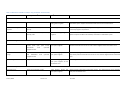
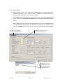
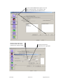
UVQ User Manual June 2010 CMIT Report No. 2005‐282 Authors Grace Mitchell Clare Diaper UVQ development team UVQ was initially developed to support the assessment of alternative urban water system scenarios within the feasibility stage of the CSIRO Urban Water Program. An existing model, AQUACYLE, was enhanced by extending the water balance model to include a number of new water flow paths and incorporating contaminant balance modelling. The UVQ development Team is: Grace Mitchell Clare Diaper Mike Rahilly Eric Dell'Oro Andrew Grant Stephen Gray Melinda Brack Trevor Farley Acknowledgements Funding for the enhancement of UVQ was provided by the EU 5FD, grant no. EVK1‐CT‐2002‐00100, Assessing and Improving Sustainability of Urban Water Resources and Systems (AISUWRS). The financial support of the Australian Government through an IAP‐International S&T Competitive Grant from the Department of Education Science and Technology (DEST) is gratefully acknowledged. The CRC for Catchment Hydrology and Grace Mitchell are acknowledged for allowing CSIRO Urban Water to access the source code of Aquacycle. Change Register Date Version Description Author/s 2007 1.1 Created Grace Mitchell Clare Diaper June 2010 1.2 Minor updates, text formatting, tutorial, screen shots Esther Coultas Stephen Cook Mike Rahilly June 2010 Version 1.2 Content Authors ...................................................................................................................................... 2 UVQ development team ............................................................................................................ 2 Acknowledgements ................................................................................................................... 2 The philosophy behind UVQ .............................................................................................. 1 Integrated water management ................................................................................................. 1 What UVQ is .............................................................................................................................. 2 The urban water and contaminant balance .......................................................................... 3 What UVQ does ......................................................................................................................... 4 Getting Started .................................................................................................................. 5 System requirements................................................................................................................. 5 Getting around UVQ .................................................................................................................. 6 UVQ Modelling Approach .................................................................................................. 6 Key concepts .............................................................................................................................. 6 Urban water system ............................................................................................................... 6 Contaminant concentrations or loads .................................................................................. 12 Temporal scale ..................................................................................................................... 13 Spatial scales ........................................................................................................................ 14 Pervious and impervious areas ............................................................................................ 18 Pervious surface areas ......................................................................................................... 18 Impervious surface areas ..................................................................................................... 18 Assumptions ............................................................................................................................ 19 Snow processes .................................................................................................................... 19 Evaporation from surfaces ................................................................................................... 20 June 2010 Version 1.2 Combined sewer systems ..................................................................................................... 20 Groundwater store ............................................................................................................... 20 Impervious surfaces ............................................................................................................. 21 Contaminants from impervious surfaces ............................................................................. 21 Pervious soil store ................................................................................................................ 21 Partial area approach .......................................................................................................... 22 2 layer soil store approach ................................................................................................... 22 Irrigation .............................................................................................................................. 22 Treatment processes ............................................................................................................ 22 Wastewater exfiltration and overflow processes ................................................................ 22 Wetting and drying of pervious and impervious surfaces ................................................... 23 Other contaminant balance assumptions ............................................................................ 23 Supply Source preferences ................................................................................................... 23 Data descriptions ............................................................................................................. 25 Project information screen ................................................................................................... 26 Physical characteristics screen ............................................................................................. 28 Water Flows screen .............................................................................................................. 31 Calibration variables ............................................................................................................ 31 Partial Area screen ............................................................................................................... 32 Snow accumulation and redistribution screen ..................................................................... 36 Land Block Water Management Features screen ................................................................ 38 Neighbourhood scale management feature screen ............................................................. 40 Study area parameters ........................................................................................................ 45 UVQ Processes ................................................................................................................. 47 Generic concepts ..................................................................................................................... 47 Conventional water system processes .................................................................................... 48 Precipitation processes ........................................................................................................ 50 Representing snowfall and snowmelt .................................................................................. 50 Main stormwater processes ................................................................................................. 51 June 2010 Version 1.2 Evaporation from impervious surfaces (Eimp) ....................................................................... 52 Non‐effective impervious surface runoff (NEAR) ................................................................. 53 Effective impervious surface runoff (IRUN) .......................................................................... 54 Pervious soil store processes ................................................................................................ 55 Excess rainfall (EXC) ............................................................................................................. 55 Actual evapotranspiration (Ea) for partial area soil store .................................................... 58 Groundwater recharge (GWR) for partial area store ........................................................... 59 Infiltration store recharge (RIS) for partial area store ......................................................... 59 Irrigation (IR) for partial area store ..................................................................................... 60 Pervious surface runoff (SRUN) for partial area store ......................................................... 61 Actual evaporation (Ea) for 2 layer store ............................................................................. 63 Upper store actual evaporation (Ea1) ................................................................................... 65 Lower store actual evaporation (Ea2) ................................................................................... 65 Drainage ............................................................................................................................... 65 Upper soil store drainage (Drain1)....................................................................................... 65 Lower soil store drainage (Drain1) ....................................................................................... 65 Groundwater recharge (GWR) for 2 layer soil store ............................................................ 66 Infiltration store recharge (RIS) for 2 layer soil store ........................................................... 66 Irrigation (IR) for a 2 layer soil store .................................................................................... 67 Pervious Surface Runoff (SRUN) for a 2 layer soil store ....................................................... 67 Groundwater process ........................................................................................................... 68 Groundwater storage (GWS) ............................................................................................... 68 Baseflow (BF) ....................................................................................................................... 68 Inflow (ISI) process ............................................................................................................... 69 Infiltration (INF) process ...................................................................................................... 69 Infiltration storage (INFS) .................................................................................................... 69 Imported water supply processes ........................................................................................ 70 Indoor water usage (IWU) ................................................................................................... 70 Leakage (LD) ........................................................................................................................ 71 June 2010 Version 1.2 Wastewater generation processes ...................................................................................... 72 Wastewater discharge (Ww) ................................................................................................ 72 Wastewater Exfiltration (EXF) .............................................................................................. 72 Overflow (OF) ....................................................................................................................... 73 Dry weather overflow (OFdry) ............................................................................................... 73 Wastewater System Capacity overflow (OFwet) .................................................................... 73 Septic Disposal ..................................................................................................................... 74 Contaminant operations .......................................................................................................... 75 Use operation ....................................................................................................................... 75 Mix operations ..................................................................................................................... 76 Sludge operations ................................................................................................................ 76 Simple sludge ....................................................................................................................... 77 Complex sludge .................................................................................................................... 78 Retained volumes ................................................................................................................. 80 Contaminant operations between spatial scales ................................................................. 80 Rainwater tank ..................................................................................................................... 81 On site wastewater store/treatment ................................................................................... 82 Garden pervious soil store ................................................................................................... 82 Public open space ................................................................................................................. 83 Neighbourhood stormwater store/treatment ..................................................................... 84 Neighbourhood Waste water store/treatment ................................................................... 85 Study area stormwater store/treatment ............................................................................. 86 Study area wastewater store/treatment ............................................................................. 87 Study area evaporation ........................................................................................................ 88 The water system variation processes .................................................................................... 89 Stormwater store operation ................................................................................................ 89 Wastewater treatment and storage operation ................................................................... 90 Aquifer store and recovery operation .................................................................................. 91 Transfer of water between neighbourhoods ....................................................................... 92 June 2010 Version 1.2 Assessing performance of a reuse scheme .......................................................................... 93 Tutorial............................................................................................................................. 93 The simulation process ............................................................................................................ 93 Data input – Conventional servicing ........................................................................................ 94 How to profile an urban area .................................................................................................. 94 Defining the spatial dimensions ........................................................................................... 94 Defining the surface area coverage ..................................................................................... 99 Defining the land block surface dimensions ......................................................................... 99 Defining the neighbourhood surface dimensions .............................................................. 100 Defining the water usage rates .......................................................................................... 101 Specifying average occupancy and indoor water usages rates ......................................... 101 Contaminants added when water is used indoors ............................................................. 102 Defining the wastewater characteristics ........................................................................... 104 Specifying the wastewater exfiltration ratio ..................................................................... 106 Estimating wastewater infiltration parameters ................................................................ 106 Estimating the surface runoff as inflow percentage .......................................................... 107 Estimating the dry weather overflow rate ......................................................................... 107 Estimating the Wastewater System Capacity .................................................................... 107 Defining the stormwater characteristics ............................................................................ 107 Estimating maximum initial loss ........................................................................................ 109 Estimating effective impervious surface area .................................................................... 109 Defining the other contaminant characteristics ................................................................ 110 Observed neighbourhood and study area flow and contaminant concentrations ............ 111 Tutorial 1: Conventional servicing ................................................................................ 114 Open the tutorial file .......................................................................................................... 114 Project Information screen ................................................................................................. 114 UVQ Main screen ............................................................................................................... 115 Physical Characteristics screen .......................................................................................... 115 Calibration Variables screen .............................................................................................. 116 June 2010 Version 1.2 Tutorial 2: Investigating alternative servicing approaches ........................................... 130 Land Block options ................................................................................................................. 130 Neighbourhood options ........................................................................................................ 132 Other Helpful hints ................................................................................................................ 137 Input File Structure ........................................................................................................ 142 Climate Input File ................................................................................................................... 142 Project File ............................................................................................................................. 142 Results............................................................................................................................ 142 Summary Statistics ................................................................................................................ 143 Technology Performance ....................................................................................................... 143 User defined graphs............................................................................................................... 143 Generated result files ............................................................................................................ 144 Cont Bal ‐ Neighbourhood N.csv ........................................................................................ 145 Cont Bal ‐ Study area.csv .................................................................................................... 146 StudyAreaBalance.csv ........................................................................................................ 146 DailyLandBlockn.csv ........................................................................................................... 148 DailyNeighbourhoodn.csv .................................................................................................. 151 MthlyNBHn.csv ................................................................................................................... 152 MthlyStudyArea.csv ........................................................................................................... 155 YearNBHn.csv ..................................................................................................................... 157 YearStudyArea.csv ............................................................................................................. 160 AISUWRS output files ............................................................................................................ 162 UFMGardenToGW.txt ........................................................................................................ 162 UFMPOSToGW.txt .............................................................................................................. 162 UFMSWInfiltrationBasinToGW.txt ..................................................................................... 162 UFMTapToGW.txt .............................................................................................................. 162 PlmUVQSWinput.txt ........................................................................................................... 163 PlmUVQWWinput.txt ......................................................................................................... 163 Worksheets .................................................................................................................... 163 June 2010 Version 1.2 Physical Characteristics of Land Blocks and Neighbourhoods ........................................... 164 Water Flow ......................................................................................................................... 165 Calibration Variables .......................................................................................................... 166 Bibliography ................................................................................................................... 168 Appendix I: Contaminant Flow Diagrams ...................................................................... 172 June 2010 Version 1.2 Table of figures Figure 1: The UVQ framework for conventional systems ................................................................ 3 Figure 2 : The conceptual representation of the urban water cycle ................................................ 4 Figure 3 : Integrated conventional urban water system .................................................................. 7 Figure 4 : An example of a residential land block .......................................................................... 14 Figure 5 : An example land block used as an industrial site. .......................................................... 15 Figure 6 : An example of a residential neighbourhood .................................................................. 16 Figure 7 : An example industrial neighbourhood. .......................................................................... 16 Figure 8 : An example study area. .................................................................................................. 17 Figure 9 : Example of stormwater and wastewater flows between neighbourhoods as represented in UVQ ................................................................................................................................................ 18 Figure 10 : Sample Project Information screen. ............................................................................. 26 Figure 11 : Sample Physical Characteristics of Land Blocks and Neighbourhoods screen. ............ 28 Figure 12 : a) Simple example of Water Flow screen b) Complex example of routing in Water Flow screen ............................................................................................................................................. 31 Figure 13 : a) Calibration Variables Partial area soil store screen b) Calibration variable 2 layer soil store screen .................................................................................................................................... 33 Figure 14 : Sample Snow Accumulation and Redistribution screen .............................................. 36 Figure 15 : Sample Land Block Water Management Features screen ........................................... 38 Figure 16 : Sample Neighbourhood Scale Management Features screen with the Stormwater & ASR tab active. ....................................................................................................................................... 40 Figure 17 : Sample Neighbourhood Scale Management Features screen with the Wastewater tab active. ............................................................................................................................................. 42 June 2010 Version 1.2 Figure 18 : Sample Neighbourhood Scale Management Features screen with the Groundwater and Imported Water tab active. ............................................................................................................ 44 Figure 19 : Sample of the Study Area Water Management Features screen. ............................... 45 Figure 20 : Water balance and contaminant balance interaction ................................................. 48 Figure 21 The conceptual representation of the urban water cycle.............................................. 49 Figure 22 : Paved area snow store. ................................................................................................ 50 Figure 23: The impervious surface runoff process. ........................................................................ 52 Figure 24 : Partial area surface store process. ............................................................................... 57 Figure 25 : The calculation of pervious surface evapotranspiration for the partial area storage method
........................................................................................................................................................ 58 Figure 26 : Pervious soil store process. .......................................................................................... 62 Figure 27: 2 layer pervious surface evapotranspiration calculation. ............................................. 64 Figure 28: Flows of contaminants to and from the road area ....................................................... 77 Figure 29 : Flows of contaminants to and from the on‐site wastewater treatment process ........ 78 Figure 30 – Rainwater tank contaminant inputs and outputs ....................................................... 81 Figure 31 – On site wastewater store contaminants inputs and outputs ...................................... 82 Figure 32 – Garden pervious soil store contaminants inputs and outputs .................................... 83 Figure 33 – Public open space soil store contaminant inputs and outputs ................................... 84 Figure 34 – Neighbourhood stormwater store contaminant inputs and outputs ......................... 85 Figure 35 – Neighbourhood wastewater store contaminant inputs and outputs ......................... 86 Figure 36 – Study area stormwater store contaminant inputs and outputs ................................. 87 Figure 37 – Study area wastewater store contaminant inputs and outputs ................................. 87 Figure 38 – Total study area evaporation contaminant inputs ...................................................... 88 Figure 39: Structure of the stormwater store ................................................................................ 90 Figure 40 : Structure of the wastewater treatment and storage unit ........................................... 91 Figure 41 : Aquifer storage and recovery system structure ........................................................... 92 Figure 42 : An example study area. ................................................................................................ 95 June 2010 Version 1.2 Figure 43 : An example industrial neighbourhood. ........................................................................ 97 Figure 44 : Heatherwood study area neighbourhoods .................................................................. 97 Figure 45 : Residential land block. ................................................................................................. 98 Figure 46 : Heatherwood project residential neighbourhood surface configuration .................. 100 Figure 47 : The Heatherwood development project stormwater and wastewater system configuration. ............................................................................................................................... 105 Figure 48 : The impervious surface runoff process. ..................................................................... 108 June 2010 Version 1.2 Table of tables Table 1 : Methods for available in UVQ for using stormwater and wastewater. .......................... 10 Table 2: Contaminant profiles required for the contaminant balance. ......................................... 13 Table 3 : Preferences in supplying a demand from multiple available sources ............................. 24 Table 4 : Project Information screen data descriptions. ................................................................ 27 Table 5 : Physical Characteristics of Land Blocks and Neighbourhoods screen data descriptions.28 Table 6 : Calibration Variables – Partial Area and 2 layer soil store screen data descriptions. ..... 33 Table 7 : Snow accumulation and redistribution screen data descriptions. .................................. 37 Table 8 : Land Block Water Management Features screen data descriptions. .............................. 38 Table 9 : Stormwater & ASR tab in the Neighbourhood scale management feature screen data descriptions. ................................................................................................................................... 40 Table 10 : Wastewater tab in the Neighbourhood scale management feature screen data descriptions. ................................................................................................................................... 43 Table 11 : Groundwater and Imported Water tab in the Neighbourhood scale management feature screen data descriptions. ............................................................................................................... 44 Table 12 : Study Area Water Management Feature screen data descriptions. ............................. 45 Table 13 : Specified contaminants and their units ......................................................................... 75 Table 14 : Simple sludge operations in UVQ .................................................................................. 77 Table 15 : Complex sludge operations in UVQ ............................................................................... 79 Table 16 : Number and area of Heatherwood land blocks. ........................................................... 99 Table 17 : Heatherwood land block pervious and impervious surface dimensions .................... 100 Table 18 : Heatherwood neighbourhood surface area dimensions ............................................. 101 Table 19 : Heatherwood indoor water usage. ............................................................................. 102 June 2010 Version 1.2 Table 20 : Heatherwood water usage contaminant values. ........................................................ 102 Table 21 : Heatherwood water system leakage parameters. ...................................................... 103 Table 22 : Heatherwood percentage irrigated area values. ......................................................... 103 Table 23 : Estimated Heatherwood irrigation values. .................................................................. 104 Table 24 : Neighbourhood wastewater configuration identifiers ................................................ 105 Table 25 : Estimated Heatherwood infiltration parameters ........................................................ 106 Table 26 : Estimated Heatherwood maximum initial loss parameters ........................................ 109 Table 27 : Estimated Heatherwood effective impervious surface parameters ........................... 109 Table 28 : Estimated Heatherwood baseflow characteristics ...................................................... 110 Table 29 : Heatherwood contaminant values. ............................................................................. 110 Table 30 : Heatherwood average volumes .................................................................................. 112 Table 31 : Observed Heatherwood contaminant concentrations................................................ 112 June 2010 Version 1.2 The philosophy behind UVQ This chapter discusses the philosophy behind UVQ. It describes: •
integrated urban water management •
what UVQ is •
what UVQ does. Integrated water management Conventional urban water management considered water supply, wastewater and stormwater as separate entities, planning, delivering and operating these services with little reference to one another. The current urban water systems harvest large volumes of water from remote catchments and groundwater sources and deliver drinking quality water to all urban uses and subsequently collect the generated wastewater. This wastewater is removed, taken to treatment plants usually located on the fringe of the city or town, where the majority is discharged to the surrounding environment. Large volumes of stormwater are also generated within urban areas due to the increased imperviousness of urban catchments. The majority of this stormwater flows out of the urban area, with some management of its quality but little attempt at collection, storage and use. As a result, the adverse impact of conventional urban water management of the water balance of these areas is substantial (Mitchell et al, 1997; 2004). In comparison, Integrated Urban Water Management takes a comprehensive approach to urban water services, viewing water supply, stormwater and wastewater as components of an integrated physical system and recognises that the physical system sits within an organisational framework and a broader natural landscape. There are a broad range of tools which are employed within Integrated Urban Water Management, including, but not limited to water conservation and efficiency; water sensitive planning and design, including urban layout and landscaping; utilisation of non‐
conventional water sources including roof runoff, stormwater, greywater and wastewater; the application of fit‐for‐purpose principles; stormwater and wastewater source control and pollution prevention; stormwater flow and quality management; the use of mixtures of soft (ecological) and hard (infrastructure) technologies; and non‐structural tools such as education, pricing incentives, regulations and restriction regimes. Integrated Urban Water Management recognises that the whole urban region down to the site scale needs to be considered, as urban water systems are complex and inter‐related. Changes to a system will have downstream or upstream impacts that will affect cost, sustainability or opportunities. Therefore, proposed changes to a particular aspect of the urban water system must include a comprehensive view of the other systems and consider the influence on them. The most important benefit of an integrated approach to urban water systems is the potential to increase the range of opportunities available in order to be able to develop more sustainable systems. In as much as the robustness of ecological systems is increased June 2010 Version 1.2 Page 1 of 176 through diversity, so too will the sustainability of urban water systems be improved if an increased range of options is made available enabling solutions to be tailored to local circumstances (Speers and Mitchell, 2000). What UVQ is UVQ is an urban water balance and contaminant balance analysis tool that was developed to: •
analyse how water and contaminants flow through an urban area, •
examine these flows from source to sink, •
highlight the interconnectedness of the water supply, stormwater and wastewater system and •
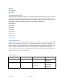
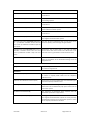
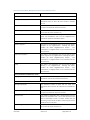
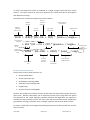
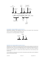
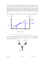
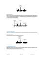
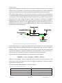
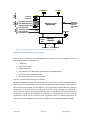
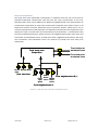
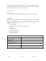
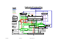
provide a tool to investigate how a wide range of non‐traditional practices enhance the urban water cycle. UVQ was initially developed to support the assessment of alternative urban water system scenarios within the feasibility stage of the CSIRO Urban Water Program. An existing model, AQUACYLE, was enhanced by extending the water balance model to include a number of new water flow paths and incorporating contaminant balance modelling. Thus, UVQ comprises two components – the water flow balance model which calculates water flows through an urban water system; and the contaminant balance model which calculates contaminant loads and concentrations throughout an urban water system. While there are several models devoted to urban water cycle modelling (see Mitchell et al, 2003), typical representations of the urban water cycle consider the man‐made and natural systems as separate entities. Within these two systems, modelling approaches generally only concentrate on one aspect of the water cycle. UVQ integrates all these networks into a single framework to provide a holistic view of the water cycle. UVQ uses simplified algorithms and conceptual routines to provide this holistic and integrated view. Figure 1 illustrates the UVQ framework and the water and contaminant flow paths represented by the model. June 2010 Version 1.2 Page 2 of 176 evaporation
rain and
snow
imported
water
evaporation
actual
evapotranspiration
road
store
roof
store
leakage
irrigation
paving
store
rainfall
excess
non-effective
area runoff (
indoor water
use
septic disposal
infiltration
store
recharge
infiltration
store
bore
extraction
wastewater
exfiltration
pervious store
pervious surface
runoff
effective impervious
surface runoff
infiltration
groundwater
recharge
groundwater
store
baseflow
inflow
overflow
stormwater
runoff
wastewater
discharge
Specified contaminant concentration
Specified contaminant load
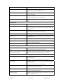
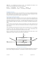
Figure 1: The UVQ framework for conventional systems The urban water and contaminant balance The technique of conducting a water balance was initially developed in the 1940's and 1950's by Thornthwaite and Mather (1955) to evaluate the importance of different hydrological parameters under a variety of hydrological conditions (Gleick, 1987). Thornthwaite and Mather (1955) applied the water balance (or budget) to gain information on periods of moisture surplus and deficit, promoting it as a basic tool for evaluation of water resources in rural areas. In the last forty years the method has evolved into detailed water balance modelling, considering either discrete events or continuous time frames. Due to the variety of disciplines applying the technique to a range of problems, the term ‘water balance’ has taken on a multitude of meanings (Thornthwaite and Mather, 1957). In regard to UVQ, the urban water balance is defined as ‘the comprehensive evaluation of the inputs, outputs and movements of water within an urban volume’. Since then, the concept of a water balance has been applied to a range of hydrological problems such as stream flow forecasting, prediction of lake and reservoir changes, irrigation demand and the assessment of human impact on the hydrological cycle June 2010 Version 1.2 Page 3 of 176 (Abdulrazzak et al., 1989). It has proved to be both flexible and readily understandable (van de Ven, 1988; Dexter and Avery, 1991). Whilst there have been a number of models developed for predicting movement of contaminants within rural areas or from urban areas to sub‐surface or open water courses, few have focused on the tracking of water borne contaminants within the existing urban environment in detail. Additionally, none examine the impacts of alternative water servicing options on the flows of contaminants within the urban environment and the effects on discharges to subsurface and open watercourses as well as to existing treatment plants and infrastructure. Water quality aspects as well as water quantity and sizing of infrastructure are essential assessment considerations for alternative water servicing options. Thus, in addition to providing an integrated approach to water servicing options in the urban environment, UVQ also provides a method for tracking water associated contaminants through the urban environment. The mapping of the contaminants in the model coincides with the mapping for the water balance. This approach allows direct representation of the effects of alterations to water services on the movement and distribution of contaminants in the urban environment. Contaminants are all modelled conservatively, with no conversion or degradation within the existing infrastructure and with simple mixing and removal processes as the basis for calculations. What UVQ does UVQ simulates an integrated urban water system within an urban area and estimates the contaminant loads and the volume of the water flows throughout the water systems from source to discharge point. It has been designed to be very flexible in the manner in which water services are represented and provides the ability to represent a wide range of conventional and more recently emerging techniques for providing water supply, stormwater and wastewater services to either an existing urban area or a site which is to be urbanized. UVQ uses the concept of an urban volume, which is a cube with unit surface horizontal area that extends from a height above the roof level to a depth below the groundwater table. Figure 2 illustrates the urban volume. precipitation
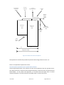
evapotranspiration
imported water
wastewater
stormwater
recharge
pumping
Urban Volume
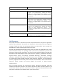
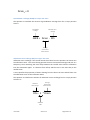
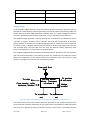
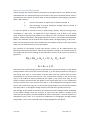
Figure 2 : The conceptual representation of the urban water cycle June 2010 Version 1.2 Page 4 of 176 This concept allows water transfers to be modelled as depths, with individual surface components accumulating or dispersing water. The concept allows the modelling of a wide range of urban forms and increased model capability. Some examples of UVQ functions are: •
provide insight into the movement of water and contaminants in the urban area •
ascertain how and where within the urban water cycle contaminants impact on the quality of water •
understand how alterations in different parts of the urban water cycle impact on the rest of the system •
estimate the impacts of different water servicing scenarios on the water cycle of planned urban development •
alter the urban form and degree of drainage connectivity and see how these actions modify the characteristics of stormwater runoff •
identify the quantity of water that may be available for reuse throughout the water cycle and the purposes for which you may reuse it •
investigate the impact of implementing demand and supply side water management actions at different spatial scales such as land block, neighbourhood and whole of study area •
tailor different mixes of servicing approaches to different portions of the study area •
investigate the relationship between the spatial pattern of demand, supply and storage capacity on the reliability of a range of alternative water sources •
provide insight into the potential consequences of implementing a number of non‐
structural changes to the system such as changing household occupancy, water usage behaviour, use of household chemical products or amount of fertiliser applied to gardens and open spaces Getting Started This chapter describes the system requirements and how to get started within UVQ. System requirements The operating system requirements for the software are: Minimum Functionality •
Operating System ‐ Windows 2000 or later. (Windows XP is preferred) •
1024x768 or higher Screen Resolution Recommended •
Small Fonts Selection for Display Adapter Settings •
Windows Regional Settings set as Australian, UK or US English Recommended •
Microsoft Excel 2000 or later ‐ English Edition for viewing output files June 2010 Version 1.2 Page 5 of 176 •
Adobe Reader 6.0 ‐ Required for Viewing the User Manual Getting around UVQ The UVQ model runs in a Windows™ environment. It uses Windows™ based screens, and navigational devices such as buttons, drop‐down menus and toolbars. UVQ Modelling Approach The chapter describes UVQ’s modelling approach. It outlines the: •
key concepts •
assumptions about the model processes Key concepts Before UVQ can simulate an urban water system, you must provide UVQ with a set of simulation parameters that characterize the urban area you want to represent. You must define the characteristics and parameters relating to the: •
Urban Water System •
Contaminant concentrations or loads •
Spatial scales •
Surface areas Urban water system UVQ simulates an integrated urban water system defined here to be: “the combined water supply, wastewater and stormwater networks the deliver water to residential, commercial, industrial and other users within an urban area, and manage the wastewater and stormwater generated within that same area”. June 2010 Version 1.2 Page 6 of 176 evaporation
precipitation
(P)
imported
water (I)
evaporation
actual
evapotranspiration
road
store
roof
store
leakage
irrigation
paving
store
rainfall
excess
non-effective
area runoff (
indoor water
use
septic disposal
pervious store
infiltration
store
recharge
infiltration
store
pervious surface
runoff
bore
extraction
wastewater
exfiltration
effective impervious
surface runoff
infiltration
groundwater
recharge
groundwater
store
baseflow
inflow
overflow
stormwater
runoff
wastewater
discharge
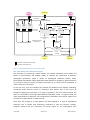
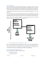
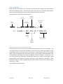
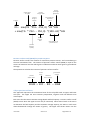
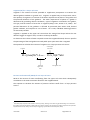
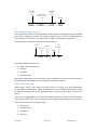
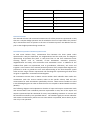
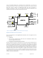
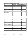
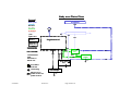
Figure 3 : Integrated conventional urban water system The UVQ model has been developed with the objective of maximum applicability to all urban areas in both Australia and Europe and so has undergone modification to include representation of a wider range of system configurations. Incorporating this flexibility into the model allows UVQ to represent: •
A variety of land use types; residential, industrial, commercial and open space. •
Different conventional water infrastructure designs such as combined sewers, septic tanks, separate stormwater systems, and groundwater bores •
Local climatic conditions Another purpose of UVQ is to represent the multitude of alternative options for water supply, stormwater and wastewater service provision, enabling the assessment of the impact of alternative water servicing approaches on the total water cycle. Options that can be represented in UVQ include: •
At land block scale – water usage efficiency, rain tanks, on‐site infiltration of roof runoff, greywater collection and sub‐surface irrigation, on‐site wastewater collection, treatment and reuse •
At neighbourhood scale – open space irrigation efficiency, aquifer storage and recovery, stormwater infiltration, stormwater collection, treatment and use and local wastewater collection, treatment and use June 2010 Version 1.2 Page 7 of 176 •
At study area/development estate scale ‐ stormwater collection, treatment and use and wastewater collection, treatment and use UVQ represents the urban water system at three spatial scales. The methods described above are provided in Table 1, with a description of some of their sources, uses and limitations. June 2010 Version 1.2 Page 8 of 176 Table 1 : Methods for available in UVQ for using stormwater and wastewater. Method #
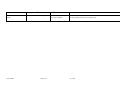
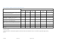
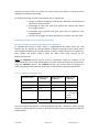
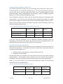
Source(s) of water Uses# Roof runoff. Kitchen, bathroom, laundry, Option to include a first flush device and divert to garden, on‐site wastewater treatment or toilet, garden irrigation stormwater system. Supplies the land block that the rain tank is located within. Comments Spatial scale: Land block Rain tank Sub‐surface greywater irrigation of One or more of kitchen, bathroom and Garden irrigation. laundry. On‐site wastewater treatment One or more of kitchen, bathroom, Toilet flushing, laundry, toilet. irrigation. Distributes greywater directly to the garden through a sub‐surface drainage field according to the daily irrigation requirement. garden Treats and stores household wastewater. Supplies the land block that it is located within. Option to dispose of effluent to leachfield, stormwater or wastewater system. Spatial scale: Neighbourhood Stormwater store Wastewater storage treatment Aquifer storage and recovery One or more of land block runoff, road Toilet flushing, garden and Option to divert a first flush to the stormwater system. A neighbourhood may service runoff, public open space runoff, open space irrigation. particular demands from its own or from another neighbourhood’s stormwater store. stormwater from upstream neighbourhoods. and One or more of land block wastewater Toilet flushing, garden and Option to disposing of overflow to stormwater or wastewater system. A neighbourhood and wastewater from upstream open space irrigation. may service particular demands from its own or from another neighbourhood’s wastewater neighbourhoods store. Neighbourhood stormwater store Toilet flushing, garden and The recharge rate and recovery rate must be specified. open space irrigation via the stormwater store Study area stormwater runoff. Toilet flushing, garden and Option to divert a first flush to stormwater system. Any neighbourhood can be supplied by open space irrigation. study area stormwater store. Spatial scale: Study Area Stormwater store January 2008 Version 1.2 10 of 191 Source(s) of water# Method Wastewater storage treatment Uses# and Study area wastewater discharge. Comments Toilet flushing, garden and Option of disposing of effluent to stormwater or wastewater system. Any neighbourhood open space irrigation. can be supplied by study area wastewater store. #
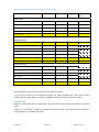
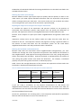
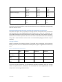
where more than one source or use is listed, any or all of the different sources/uses can be selected by the user. January 2008 Version 1.2 11 of 191 Contaminant concentrations or loads The mapping of contaminants in the model coincides with the mapping for the water balance, thus directly representing the way in which alterations in the water flows affect the movement and distribution of contaminants. This is a simplification of the processes that occur and does not consider temporal variations in water quality. As UVQ models at a daily time step this approach is applicable and provides detail on sources and flows of contaminants. In addition, as the majority of data collected on temporally varying contaminants flows in the urban environment is expressed as event mean concentrations, this approach is suitable. During the development of the UVQ software an extensive literature review of reported values for water related contaminant loads and concentrations was undertaken. Table 2 lists the contaminant sources considered in the model. Variability in the load or concentration from each source arises from land use and source characteristics and depending on data availability, certain assumptions can be made. UVQ software developers realized the data hungry nature of the model and that collecting data from case study sites for all the streams required in the contaminant balance is an onerous task. Thus, literature values for many input streams can be used where appropriate and where data for the area being modelled is not available. The method of describing contaminant loads from sources also allows different systems to be analysed, as flows from various sources can be combined, diverted or treated separately. The assigning of contaminant loads as input to the indoor water use sources also allows the model to effectively deal with water recycled to the house, as the load is independent of the quality of water used. June 2010 Version 1.2 Page 12 of 176 Table 2: Contaminant profiles required for the contaminant balance. Contaminant Source Residential Commercial Industrial Public space Water Supply 9 9 9 9 Bore Water (Local ground water) 9 9 9 9 Precipitation 9 9 9 9 Evaporation 9 9 9 9 Rainwater tank 9 9 9 Greywater 9 9 9 Kitchen 9 9 9 Bathroom 9 9 9 Laundry 9 9 9 Toilet 9 9 9 Neighbourhood WWTP effluent 9 9 9 On‐site WWTP effluent 9 9 9 Roof 9 9 9 Roof first flush 9 9 9 Roads 9 9 9 Paved areas 9 9 9 Fertiliser application 9 9 9 9 Neighbourhood stormwater effluent 9 9 9 9 open Water Stream Wastewater Stream Stormwater Stream Note: Yellow cells in table denote data for contaminant balance calibration rather than model input Rural open space requires the same data as for public open space. To track the movement of contaminants through the urban landscape, the water flow volumes calculated by the water balance model are combined with contaminant concentration data. Temporal scale UVQ uses a daily time step for computation, with the model output summed to monthly and annual totals. UVQ uses a climate file to define the temporal period simulated. The maximum time period of a single simulation is limited to 100 years. June 2010 Version 1.2 Page 13 of 176 Spatial scales UVQ uses three spatial scales to represent the urban area. The land block scale, the neighbourhood scale and the study area scale. UVQ requires the configuration parameters of each spatial scale before it can simulate the urban area. Landblock
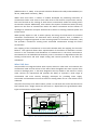
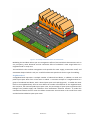
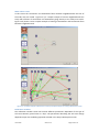
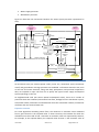
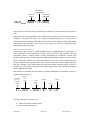
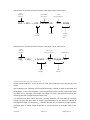
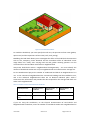
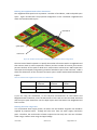
A land block represents a single property that may contain building(s), paved areas, and garden areas. A common example of a land block is a residential property that contains a house, driveway, and garden (Figure 4). For the water balance the user must specify the water usage per occupant for kitchen bathroom, laundry and toilet end uses, the total block area, roof area, paved area and garden area, the occupancy of the household and the percentage of garden area irrigated. For the contaminant balance the user must specify input loads of contaminants to the laundry, kitchen, bathroom and toilet, fertiliser load to the garden and the quality of roof runoff, pavement runoff, drinking water and rainwater. Figure 4 : An example of a residential land block Land blocks may also represent commercial, industrial or institutional sites such as a factory or a school and the configuration of the land block will change based on how the land block is used. A land block containing an industrial property, for example, may only contain a factory building and car parking areas. Figure 5 illustrates a typical land block used as an industrial site. The user specified values of roof area, paved area and garden area and contaminant loads and concentrations will be significantly different from a residential block. June 2010 Version 1.2 Page 14 of 176 Figure 5 : An example land block used as an industrial site. Modelling the land block allows you to investigate the effect of the land block characteristics such as size, occupancy, water demands and the cumulative effect of individuals’ water usage habits on a neighbourhood or study area. The land block is the smallest management scale possible for water supply, stormwater runoff, and wastewater disposal which is why it is a useful fundamental spatial scale for this type of modelling. Neighbourhood
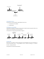
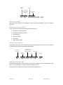
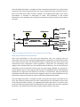
A Neighbourhood represents a multiple number of identical land blocks, in addition to roads and public open space which form a local area or suburb. A common example of a neighbourhood is a group of residential land blocks, with a shared open space and roads (Figure 6). To model the water flows in the neighbourhood, the user must define the number of land blocks in the neighbourhood, the total area, the road and pubic open space areas, the percentage of open space irrigated and the leakage from potable supply and exfiltration from wastewater collection network. To model the contaminant balance the user must also define contaminant concentration in the runoff from roads and the fertiliser added to open space areas. June 2010 Version 1.2 Page 15 of 176 land block
open space
road area
Figure 6 : An example of a residential neighbourhood Alternatively, the land blocks in the neighbourhood could be used for commercial, industrial or institutional purposes. A neighbourhood that simulates an industrial area may only contain industrial land blocks and roads (Figure 7). A neighbourhood that simulates an area used for institutional purposes such as large university campuses may contain the institutional land blocks, a number of open spaces and roads. Alternatively, a neighbourhood may contain solely open space or solely roads or solely land blocks. Figure 7 : An example industrial neighbourhood. Modelling the neighbourhood allows you to investigate the impact of alternate water management options for a neighbourhood and how the demand for water changes according to the pattern of the relevant land use. There is also the opportunity to represent the behaviour of a cooperative group of land blocks which share a stormwater storage facility or wastewater treatment plant. June 2010 Version 1.2 Page 16 of 176 The land block scale functions still occur when modelling at the neighbourhood and study area scale, but they occur within the land block section of the model. Varying land use and garden watering patterns are accounted for at the land block scale within a neighbourhood. Studyarea
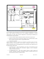
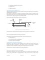
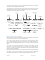
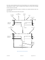
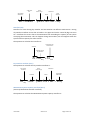
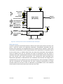
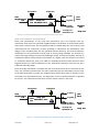
A study area represents an urban area containing a number of neighbourhoods that have mixture of land uses such as residential, industrial, commercial and institutional. These neighbourhoods may relate to the suburbs in the study area or areas of single land use. An example of a study area containing residential, commercial and industrial neighbourhoods is shown in Figure 8. Figure 8 : An example study area. To model a study area you must identify the number of neighbourhoods that make up the study area and the configuration characteristics of each neighbourhood within the study area. Modelling a study area allows you to investigate the cumulative effect of different water management strategies within the neighbourhoods within a study area or to explore the feasibility of having different water systems within neighbourhoods that have different characteristics. The study area is used within the model to represent the spatial scale at which suburban or city water supply and water disposal operations are managed. The drainage networks linking neighbourhoods, in terms of the flow of stormwater and wastewater can be stated, allowing the spatial relationship between neighbourhoods to be represented and the way in which stormwater and wastewater flow though the study area (Figure 9). June 2010 Version 1.2 Page 17 of 176 Figure 9 : Example of stormwater and wastewater flows between neighbourhoods as represented in UVQ Pervious and impervious areas In the modelling approach used in UVQ two types of surface are represented, pervious and impervious. Pervious surface areas Pervious areas are any areas where water penetrates and re‐distributes into the soil through infiltration, such as gardens, parks and open spaces. There are two conceptual representations of pervious surface areas and their underlying pervious soil; 1. partial area approach 2. two layer approach See the UVQ Processes chapter for an explanation of how these two soil store representations differ. Impervious surface areas Impervious surface areas are areas where water does not infiltrate through the surface. They are divided into three separate surfaces within each neighbourhood: •
roads, •
roofs and •
paved areas June 2010 Version 1.2 Page 18 of 176 The redistribution of water from these surfaces requires some understanding of the surface types, their location in the study area and their physical characteristics. The concept of an effective paved, road or roof area is used to describe the percentage of impervious area connected directly to the drainage system. The remaining non effective area drains to the pervious surfaces. The concept of maximum initial loss is used to estimate the amount of incident water required to wet an impervious surface prior to runoff commencing. These concepts are described further in UVQ Processes and Data descriptions. Assumptions A number of assumptions are associated with UVQ and the representation of: •
Snow processes •
Evaporation from surfaces •
Combined sewer systems •
Groundwater store •
Impervious surfaces •
Contaminants from impervious surfaces •
Pervious soil store •
Partial area •
2 layer soil store •
Irrigation •
Treatment processes •
Surface types in road and open space •
Wastewater exfiltration and overflow processes •
Wetting and drying of pervious and impervious surfaces •
Contaminant flows and loads •
Water supply sources The assumptions associated with these different processes are described in the following sections. Snow processes • Precipitation falls either as all snow or all rain on any given day, depending on the average daily temperature and the user specified snowfall threshold temperature •
There is no variation in snowfall threshold temperature and melt rate factor due to variations in elevation within the study area. The effect of elevation variations is assumed to be minimal •
There is no variation in melt rate factor due to season, snow condition or snow density •
The melt rate factor represents the water depth equivalent amount of snow •
Snow automatically accumulates in garden and open space surfaces. The user can specify whether there is accumulation on paved, roof and road surfaces. •
Rainfall passes straight through the snow pack onto the surface below June 2010 Version 1.2 Page 19 of 176 Evaporation from surfaces • The effect of wind turbulence due to increased surface roughness, sheltering by buildings, and other microclimate variations due to urbanisation, does not have a significant impact on the accuracy of the method used to calculate actual evapotranspiration from pervious areas and evaporation from impervious areas. There is little known about the actual difference between urban and non‐urban evapotranspiration. •
Actual evapotranspiration of pervious areas varies depending on the soil moisture storage at the beginning of the day, and the evaporative demand estimated by potential evapotranspiration as supplied in the climate input file. This accords with the approach of Boughton (1966) (a simplified Denmead and Shaw (1962) relationship) given in Equation 12. •
The presence of a layer of snow covering a particular surface (garden, public open space, roof, road, paved) does not alter the calculation of actual evapotranspiration from these surface stores •
The maximum rate of evaporation from impervious surfaces is assumed as the potential evapotranspiration as supplied in the climate input file. No allowance is made for the effect of heating of impervious surfaces on the actual evaporation rate. Evaporation is removed from the impervious surface store at the end of the day (effectively after the rain event). •
The concentration of evaporated contaminants is assumed to be the same from all surfaces. Evaporation of all contaminants can be set to zero. Contaminants evaporate from surface stores on all impervious surfaces and from subsurface stores of pervious surfaces. Combined sewer systems • Each neighbourhood can have either a separate or combined sewer system •
In a neighbourhood with a combined sewer system, all of the surface runoff generated from impervious surfaces in that neighbourhood (which has not been intercepted and utilised by rainwater tanks or stormwater stores) is directed into the wastewater system. • The parameter percentage surface runoff as inflow should be set to 100%. • The ‘Wastewater System Capacity’ should be enabled and set to 0kL. •
Base flow from the groundwater store flows onto the stormwater system, regardless of whether a separate or combined sewer system is selected in a neighbourhood. •
Stormwater flowing into a neighbourhood from an upstream neighbourhood stays in the stormwater system (this can be used to represent streams and creeks flowing through a neighbourhood). •
Overflows from a combined sewer system are directed into the neighbourhood’s stormwater system Groundwater store • The groundwater store is assumed to be an unconfined aquifer. •
Groundwater recharge spreads uniformly over the entire groundwater store below a neighbourhood; transmisivity is assumed to be infinite. This assumption has little effect on model accuracy unless there is a large amount of water recharging at a fixed point within the modelled area. Any impact on base flow estimation is not significant and does not warrant more sophisticated modelling of the groundwater store. June 2010 Version 1.2 Page 20 of 176 •
There is no deep seepage from the groundwater store. The groundwater store is an infinite source of water and the only discharge from the store is though base flow and/or extraction by a bore. Impervious surfaces • All roof, paved and road area is 100% impervious. •
The maximum initial loss from an impervious surface and the effective impervious area are assumed to be constant throughout a rain event and for all seasons during a year. •
The runoff from unconnected impervious areas is assumed to spread evenly across the entire adjacent pervious area (therefore being added to both pervious stores in equal areal depths). Roof and paved area runoff spills onto the pervious area within the same land block. Any road runoff from unconnected areas (non‐effective area) spills onto all pervious area within the neighbourhood. In actuality, the runoff would spill onto the edge of the adjacent pervious area and cause an increase in the moisture content of a small area. •
If there is no pervious area adjacent to an impervious area, then the effective impervious area is 100%. All of the impervious surface must be directly connected to the stormwater system since there are no adjacent surfaces for the runoff to spill on to. Contaminants from impervious surfaces • Contaminant concentrations in the runoff from the garden and public open space are calculated separately from respective input loads •
Contaminant concentrations in the runoff from the pavement to the garden or stormwater are identical •
No contaminant load is added to stormwater from impervious surfaces but the model calculates the difference between rainfall and stormwater EMCs (event mean concentrations) to provide users with an indicator of this load Pervious soil store • All public open space is 100% pervious •
The input and output of water occurs in a set order each day. Precipitation is added to and actual evaporation is removed from the soil moisture stores simultaneously at the beginning of the day. The irrigation demand is calculated and is applied at the end of the day (for more details of the algorithms describing the soil store see UVQ Processes). •
Precipitation and irrigation wet the entire root zone to a constant level. This assumes the moisture is instantaneously distributed throughout the root zone when, in reality, a wetting front forms and the soil is slow to reach a constant soil moisture level throughout. •
Surface ponding and overland flow do not occur until the soil moisture storage capacity of the store is exceeded. This may over‐estimate the ability of precipitation and irrigation to wet the soil profile and underestimate runoff in intense rainfall events when infiltration capacity of the soil profile is exceeded. •
There is no lateral movement of moisture in the soil profile. Therefore, there is no transfer of moisture between the soil and groundwater stores in different neighbourhoods. •
All soil below impervious surfaces is regarded as dry. •
If there is no garden on the land block, there can be no leach field associated with a septic tank. June 2010 Version 1.2 Page 21 of 176 •
The removal of contaminants by the pervious soil store is specified by the user as a percentage •
Contaminant concentrations in runoff from the garden and public open space are calculated separately from their different input loads Partial area approach Assumptions specific to the partial area approach are: •
There is no transfer of moisture between the two pervious stores. •
Any moisture in excess of either of the two partial area soil storages capacity overflows the store and is separated into surface runoff, groundwater recharge, and infiltration into the wastewater system according to user defined calibration parameters. •
The septic tank system leach field drains into both soil stores. If there is no garden on the land block, there can be no leach field. 2 layer soil store approach Assumptions specific to the 2 layer soil store approach are: •
Any water entering the upper soil store, in excess of capacity, becomes runoff. •
Irrigation is applied to the upper soil store only. •
Drainage of the soil stores behaves like a simple decay function •
The septic tank system leach field drains into the lower soil store. •
The spoon drain routes water into the lower soil store. •
Infiltration is a constant proportion of the drainage from the lower soil store. Irrigation • The model assumes irrigation to be fully effective in recharging the soil moisture stores to the prescribed level with no wastage. In reality part of the water applied to a garden or open space will be wasted as some will evaporate before soaking into the soil, depending on the timing of irrigation and the method used. •
All outdoor water use is due to irrigation of either gardens or public open space. Treatment processes • All treatment processes are modelled as continuously stirred tank reactors (CSTRs) and contaminant removal is described as a percentage •
Sludge accumulates in the treatment process •
Treatment process calculations occur on a daily basis and the retained volume and contaminants from the previous day are the starting volume and contaminants for the current day. The retained volume and contaminants reported in results screens are for the final day only Wastewater exfiltration and overflow processes • Exfiltration from the wastewater network is a constant proportion of the generated wastewater flow. •
Wastewater overflow is comprised of two components; dry weather overflow and Wastewater System Capacity (formerly labelled wet weather overflow). Dry weather overflow is a constant proportion of generated wastewater flow up to capacity flow levels. June 2010 Version 1.2 Page 22 of 176 Wastewater System Capacity is all generated wastewater flow in excess of the system capacity. •
Contaminant concentration in exfiltration stream is the same as that in the flow in the wastewater network Wetting and drying of pervious and impervious surfaces • Only one wetting and drying cycle occurs within a day. In reality, there may be multiple wetting and drying cycles, due to multiple rain events occurring within the day •
Precipitation is spread evenly over the entire area with no variation due to wind turbulence and localised storms. Other contaminant balance assumptions • Specified contaminant loads have no associated water volume Supply Source preferences If there is more than one source selected to supply a particular demand (e.g. both rain tank and on‐
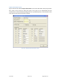
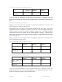
site wastewater treatment unit) then there is a set order in which these sources will be used to meet that demand. The rules used to determine the priorities for each demand are as follows: 1. Use the lowest quality water source available which meets the requirements of the demand first. 2. Supply indoor water demands before outdoor demands. 3. Use the water sources within the land block before neighbourhood sources. 4. Use neighbourhood scale water sources before study area scale water sources. 5. Use all local sources of water before importing water (reticulated water). If a particular potential source of water has not been selected by the user, then the next highest priority source is used instead. June 2010 Version 1.2 Page 23 of 176 Table 3 : Preferences in supplying a demand from multiple available sources Water Supply source Water Demand Land block kitchen Land block bathroom Land block laundry Land block toilet Land block irrigation Neighbourhood public open space irrigation 1 1 2 Land block rain tank 1 1 1 2 3 Neighbourhood wastewater store (located in own Neighbourhood or another Neighbourhood) 3 4 1 Neighbourhood stormwater store (located in own Neighbourhood or another Neighbourhood) 4 5 2 Aquifer storage and recovery (via Neighbourhood stormwater store) 4α 5α 2α Study area wastewater store 5 6 3 Study area stormwater store 6 7 4 2β 2β 2β 7β 8 5 Land block direct sub‐surface greywater irrigation (kitchen and/or bathroom and/or, laundry) water Reticulation α
: Aquifer storage and recovery operates in conjunction with a Neighbourhood scale stormwater store (see Aquifer store and recovery operation section), β
: Reticulated water is automatically supplied to Land block indoor water demands if there is a shortfall in supply from higher priority sources. June 2010 Version 1.2 Page 24 of 176 Data descriptions There are eight input screens in UVQ, each requiring specific data about the area to be modelled. The screens have been formatted so that related information is grouped on one screen. The screen descriptions are as follows: •
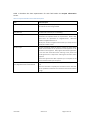
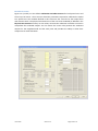
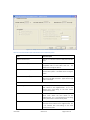
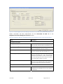
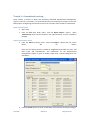
Project Information screen – details generic information relevant to the whole project area to be modelled •
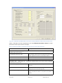
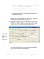
Physical Characteristics (Physical characteristics of land blocks and neighbourhoods) screen – details pervious and impervious areas in both land blocks and neighbourhood and associated water flows and contaminant loads or concentrations •
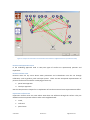
Water Flow (Neighbourhood wastewater and stormwater flow links) screen – details the wastewater and stormwater flows between neighbourhoods •
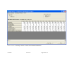
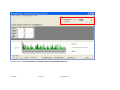
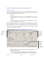
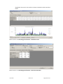
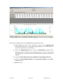
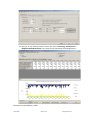
Calibration Variables screen – details the calibration parameters required for the pervious and impervious surfaces and the wastewater system. In addition, this screen can be used to compare simulated stormwater and wastewater flows and concentrations with observed values (part of the calibration process see Tutorial ) •
Snow variables (snow accumulation and redistribution) screen – details the temperature thresholds and accumulation and redistribution variables required to simulate the snow processes •
Land Block (land block water management features) screen – details the physical characteristics, supply and usage options and process efficiencies for land block raintank and on‐site wastewater treatment systems •
Neighbourhood (neighbourhood water management features) screen ‐ details the physical characteristics, supply and usage options and process efficiencies of neighbourhood stormwater, wastewater and groundwater storage and treatment options •
Study Area (study area water management features) screen ‐ details the physical characteristics, supply and usage options and process efficiencies of study area stormwater and wastewater storage and treatment options. June 2010 Version 1.2 Page 25 of 176 Project information screen Figure 10 shows the default Project Information screen which describes overall project data. This screen can be used to select the type of soil store to be represented and the contaminants to be simulated (including three user specified options). Further details of the user input to this screen are found in Tutorial. Figure 10 : Sample Project Information screen. June 2010 Version 1.2 Page 26 of 176 Table 1 describes the data requirements for each field within the Project Information screen. Table 1 : Project Information screen data descriptions. Field Data Description Project Description Brief description of the project. Max. 32 characters. This is usually the name of the area being modelled. Study Area Size The total area of the site you are modelling Number of Neighbourhoods A study area is divided into zones that have similar surface area dimensions and imported water use requirements. Within UVQ, these zones are represented as neighbourhoods. Maximum number of neighbourhoods is 75. Identify the number of neighbourhoods within your study area and specify the number of here. Soil Store Type The two conceptual models of pervious surface soil stores within rainfall runoff models are the partial area runoff approach or the saturation excess approach. UVQ supports both these approaches. It uses the term Partial Area when referring to the partial area runoff approach and 2 Layer when referring the saturation excess approach. Choose the approach that best represents your conception of the surface soil store within your study area. Contaminants for Analysis in this Study Select the contaminants you wish to represent within your study Area, Neighbourhoods and Land Blocks area. Select the check box and specify the contaminant in the data field. All user specified contaminants are assumed to have concentrations in mg/l June 2010 Version 1.2 Page 27 of 176 Physical characteristics screen Figure 11 is a sample of the default Physical Parameters of land block and Neighbourhood screen. In this screen the physical characteristics of both the land block and the neighbourhood are described. In addition, data on the water usage for the four main household indoor uses, toilet, bathroom, laundry and kitchen and the associated contaminant loads is required. This segregation of end uses allows simulation of different recycled water streams and qualities to the different end uses. This screen also details all the specified contaminant data required to complete the simulation. Figure 11 : Sample Physical Characteristics of Land Blocks and Neighbourhoods screen. Table 2 describes the data requirements for the Physical Parameters of land block and Neighbourhood screen. Table 2 : Physical Characteristics of Land Blocks and Neighbourhoods screen data descriptions. Field Data Description Neighbourhood frame Total Area (ha) The neighbourhood spatial scale represents a number of individual properties and any associated roads and public open space. The total area of a neighbourhood is the sum of the open space areas, road areas and the individual properties within the neighbourhood. User input of this value provides a cross check that other areas within the neighbourhood have been specified correctly. Road Area (ha) The number of hectares of roads within a neighbourhood Note: the road area is the sum of the roads and the footpaths. June 2010 Version 1.2 Page 28 of 176 Field Data Description Open Space Area (ha) The number of hectares of open space such as parks, wildlife corridors and so on within a neighbourhood Percentage of Open Space Irrigated (%) The percentage of the open space irrigated. The whole area may or may not be irrigated. Imported Supply Leakage (%) The percentage of the imported water that leaks into the groundwater through broken and cracked pipes. Wastewater as Exfiltration (ratio) The ratio of wastewater exfiltrating (leaking) from the wastewater pipes. Land Block frame Number of Land Blocks Total number of identical land blocks within this neighbourhood. Block Area (m2) UVQ treats land blocks within a neighbourhood homogeneously. You must specify the average size of the land blocks within your neighbourhood. Average Occupancy Average number of people using water indoors within the land block. UVQ accepts whole and decimal numbers. Garden Area (m2) The average garden area within the average land block. Roof Area (m2) The average roof area including sheds and garages within the average land bock. Paved Area (m2) The average paved area within the average land bock Percentage of Garden Irrigated (%) The percentage of the garden area that is irrigated. The whole area may not or may not be irrigated. Roof Runoff to Spoondrain (ratio) The ratio of total roof runoff that drains into an on‐site soak‐away. Indoor Water Usage & Contaminants frame Bathroom, Toilet, Kitchen and Laundry Specify the number of litres of water used per person per day L/c/d within the bathroom, toilet, kitchen and laundry. Bathroom, Toilet, Kitchen and Laundry Specify the average contaminant loads due to householders in the Contaminant Loads mg/c/d bathroom, toilet, kitchen and laundry within a land block. Other Contaminants frame Imported (mg/L) Specify the contaminant concentration of the water imported into the neighbourhood. This value is used for all imported water to the study area. Rainfall (mg/L) Specify the contaminant concentration of the rainfall throughout the neighbourhood. This value is used for all rainfall in the study area. Pavement Runoff (mg/L) Specify the average contaminant concentration of the pavement runoff within your average land block. Roof Runoff (mg/L) Specify the average contaminant concentration of the average roof runoff within an average land block. Road Runoff (mg/L) Specify the event mean contaminant concentrations of the road runoff in a neighbourhood. June 2010 Version 1.2 Page 29 of 176 Field Data Description Roof First Flush (mg/L) The roof first flush is the water that is prevented from entering a rain water tank to prevent pollutants from entering the tank. The first flush runoff may carry more pollutants in it than the following runoff. Specify the average contaminant concentrations of the roof first flush within an average land block. Fertiliser to POS (mg /ha/day) Specify the contaminant loads of fertiliser used on the public open spaces within the neighbourhoods. Evaporation (mg/L) Specify the contaminant concentrations of evaporated water from all surfaces within the neighbourhood. Contaminant evaporation from all surfaces is assumed the same. Groundwater (mg/L) Specify the contaminant concentration of the groundwater (bore water) leaving the groundwater store within a neighbourhood. Fertiliser to garden (mg /m2/day) Specify the contaminant loads within the fertiliser used on the gardens within land blocks. Water Outputs frame Wastewater from Neighbourhood goes The identification number of the neighbourhood into which the to: wastewater from this neighbourhood flows. The wastewater flows paths are set up and implemented in the Water Flow screen and so the value in this screen cannot be edited. Stormwater from Neighbourhood goes to: The identification number of the neighbourhood into which the stormwater from this neighbourhood flows. The stormwater flows paths are set up and implemented in the Water Flow screen and so the value in this screen cannot be edited. June 2010 Version 1.2 Page 30 of 176 Water Flows screen In this screen the stormwater and wastewater flows between neighbourhoods and out of the study area are routed. Figure 12 a) is a simple example of a three neighbourhood case study with all flows of stormwater and wastewater going directly to the study area outlet. Figure 12 b) shows a more complex example of routing of wastewater and stormwater flows between neighbourhoods. Figure 12 : a) Simple example of Water Flow screen b) Complex example of routing in Water Flow screen Calibration variables The calibration variable screen will contain different parameters dependent of the type of soil store selection, partial area or 2 layer. The parameters describing the soil store change dependent upon the modelling approach selected in the Project Description screen June 2010 Version 1.2 Page 31 of 176 Partial Area screen Figure 13 a) and b) are the default Calibration Variables Screens for both partial area and the 2 layer soil stores. These screens detail the parameters required to calibrate the model to a specific site. The variables defined in this screen are the ‘controls’ for the output flows and concentrations. The physical characteristics of the area to be modelled (as defined in the Physical Characteristics screen) are set values, whereas the calibration variables are used to manipulate the simulated outputs. For this reason this screen also presents the simulated outputs for the neighbourhood and the study area and provides the ability to allow their comparison to observed values. June 2010 Version 1.2 Page 32 of 176 Figure 13 : a) Calibration Variables Partial area soil store screen b) Calibration variable 2 layer soil store screen Table 3 describes the data requirements for the Calibrated Parameters Screen for both partial area and 2 layer soil store concepts. Table 3 : Calibration Variables – Partial Area and 2 layer soil store screen data descriptions. Field Description Stormwater frame – partial area (Figure 13 : a) Calibration Variables Partial area soil store screen b) Calibration variable 2 layer soil store screen Percentage Area of Soil Store 1 (%) The proportion of the pervious area (garden and open space) in the neighbourhood which is covered by Soil Store 1. Capacity of Soil Store 1 (mm) The maximum depth of water Soil Store 1 can store. Capacity of Soil Store 2 (mm) The maximum depth of water Soil Store 2 can store. Stormwater frame – 2 layer (Figure 13 : a) Calibration Variables Partial area soil store screen b) Calibration variable 2 layer soil store screen Maximum Soil Storage Capacity (mm) The maximum depth of water the upper and lower soil store can hold. Soil Store Field Capacity (mm) The level to which the water in the upper and lower soil store freely drains due to the action of gravity. Maximum Daily Drainage Depth (mm) The maximum depth of water which will drain from the upper and lower soil store in a day due to the action of gravity. June 2010 Version 1.2 Page 33 of 176 Field Description Roof Area Maximum Initial Loss (mm) The amount of water it takes to wet the roof surface before runoff occurs. Effective Roof Area (%) The proportion of roof area which is directly connected to the roof drainage system. Paved Area Maximum Initial Loss (mm) The amount of water it takes to wet the paved surface before runoff occurs. Effective Paved Area (%) The proportion of paved area which is directly connected to the land block stormwater system. Road Area Maximum Initial Loss (mm) The amount of water it takes to wet the road surface before runoff occurs. Effective Road Area (%) The proportion of road area which is directly connected to the neighbourhood stormwater system. Base Flow Index (ratio) for partial area (Figure The ratio of water overflowing from the soil stores due to 13 : a) Calibration Variables Partial area soil excess in capacity, which recharges the groundwater. store screen b) Calibration variable 2 layer soil store screen Drainage Factor (ratio) for 2 layer (Figure 13 : a) Controls the rate at which water in the upper soil stores Calibration Variables Partial area soil store drains into the lower store and the rate at which water in the screen b) Calibration variable 2 layer soil store low store drains to groundwater and the infiltration store. screen Base Flow Recession Constant (ratio) Controls the rate in which water leaves the groundwater store and contributes to the stormwater flowing out of the neighbourhood. Contaminant Soil Store Removal % Highlighted contaminants The percentage of the contaminant removed from the water as it drains through the soil. Wastewater Infiltration Index (ratio) The proportion of water overflowing from the soil stores due to excess in capacity which flows into the temporary infiltration store. Infiltration Store Recession Constant (ratio) Controls the rate in which water flows into wastewater pipes from the temporary infiltration store. Percentage Surface Runoff as Inflow (%) Proportion of surface runoff generated in the neighbourhood which flows into the wastewater pipe system rather that the stormwater system. Dry Weather Overflow Rate (%) The proportion of wastewater which overflows from the wastewater system due to pipe chokes. Wastewater System Capacity (kL) The trigger represents the maximum amount of wastewater the neighbourhood wastewater system can convey each day. All wastewater flowing into the wastewater system in excess of this capacity then becomes overflow. June 2010 Version 1.2 Page 34 of 176 Field Description Irrigation frame Garden Trigger to Irrigate This is a ratio value between 0 and 1, representing the level of soil wetness that the garden irrigator wishes to maintain. If the soil water storage level in the proportion of the garden that is irrigated drops below this trigger level then irrigation water is requested from the various sources available to it. Open Space Trigger to Irrigate This is a ratio value between 0 and 1, representing the level of soil wetness that the open space irrigator wishes to maintain. If the soil water storage level in the proportion of the open space that is irrigated drops below this trigger level then irrigation water is requested from the various sources available to it. Average Volumes frame ‐ This Neighbourhood tab KL/y Option of displaying observed and simulated imported water, stormwater and wastewater flow results as kL/y or ML/y Observed Imported Measured volume of water imported into the neighbourhood. This is a user defined parameter and should be obtained from actual site data if possible. It represents the value that UVQ should replicate when the calibration parameters values are set correctly. Observed Wastewater Measured volume of wastewater leaving the neighbourhood. This is a user defined parameter and should be obtained from actual site data if possible. It represents the value that UVQ should replicate when the calibration parameters values are set correctly. Observed Stormwater Measured volume of stormwater leaving the neighbourhood. This is a user defined parameter and should be obtained from actual site data if possible. It represents the value that UVQ should replicate when the calibration parameters values are set correctly. Simulated Imported UVQ’s calculated volume of water imported into the neighbourhood. It provides a guide to how well the calibration parameters defined on this screen are simulating the observed volume of imported water. Simulated Wastewater UVQ’s calculated volume of wastewater leaving the neighbourhood. It provides a guide to how well the calibration parameters are simulating the observed volume of stormwater. Simulated Stormwater UVQ’s calculated volume of stormwater leaving the neighbourhood. It provides a guide to how well the calibration parameters are simulating the observed volume of wastewater. Quality frame ‐ This Neighbourhood tab Concentration or Load June 2010 Provides the option of using the units of concentration (mg/l) or loads (kg/yr) for observed and simulated imported water, stormwater and wastewater contaminants. Version 1.2 Page 35 of 176 Field Description Wastewater Observed Contaminants Measured event mean concentrations or loads of selected wastewater contaminants leaving the neighbourhood. This is a user defined parameter and should be obtained from actual site data if possible. It represents the value that UVQ should replicate when input and calibration parameter values are set correctly. Stormwater Observed Contaminants Measured concentrations or loads of selected wastewater contaminants leaving the neighbourhood. This is a user defined parameter and should be obtained from actual site data if possible. It represents the value that UVQ should replicate when input and calibration parameter values are set correctly. Simulated Wastewater UVQ’s calculated concentration or load of contaminants leaving the neighbourhood in the wastewater. It provides a guide to how well the set of input parameters are simulating the observed concentrations or loads of stormwater. Simulated Stormwater UVQ’s calculated concentration or load of contaminants leaving the neighbourhood in the stormwater. It provides a guide to how well the set of input parameters are simulating the observed concentrations or loads of stormwater. Snow accumulation and redistribution screen Figure 14 is the default Snow accumulation and redistribution screen. This screen is used to select the threshold temperatures for snowfall and snow melt and to define the impervious areas where snow collects and the impervious areas to which snow distributes. Please note, the redistribution process is not available in this version of UVQ. Table 4 describes the data requirements for the Snow accumulation and redistribution screen. June 2010 Version 1.2 Page 36 of 176 Figure 14 : Sample Snow Accumulation and Redistribution screen Table 4 : Snow accumulation and redistribution screen data descriptions. Field Data Description Simulate Snow Process Switches on or off the routines in UVQ which simulate snow. Snowfall threshold (oc) The threshold daily mean temperature at which precipitation falls as snow rather than rain. The default value is 0 degrees Celsius. Snow Melt Threshold (oc) The threshold daily mean temperature at which snow that has built up melts. The default value is 0 degrees Celsius. Melt Rate Factor (mm/oc/d) The rate at which snow melts when the temperature is above the Snow Melt Threshold. Typical values range from 2 to 10 mm/d. Accumulation frame Roads in neighbourhood When this option is selected, snow builds up on the road surfaces in the neighbourhood. If it is not selected then snow falling on the road surface instantaneously melts. Paved area in land block When this option is selected, snow builds up on the paved areas within the land blocks of the neighbourhood. If it is not selected then snow falling on the paved surfaces instantaneously melts. Roofs in land block When this option is selected, snow builds up on the roof within the land blocks of the neighbourhood. If it is not selected then snow falling on the roofs instantaneously melts. June 2010 Version 1.2 Page 37 of 176 Field Data Description Redistribution frame – not available in this version of UVQ Paved Area to garden If this option is selected, snow that falls on the paved area within a land block is removed to the garden within that land block. Road to open space If this option is selected, snow that falls on the roads within the neighbourhood is removed to the user selected open space area, either within that neighbourhood or another neighbourhood. Road to outside study area If this option is selected, snow that falls on the roads within the neighbourhood is removed to outside the study area. Paved area redistribution threshold (mm) Defines the depth of snow which can accumulate on the paved area before action is taken to remove the snow. Road area redistribution threshold (mm) Defines the depth of snow which can accumulate on the road surfaces before action is taken to remove the snow. Land Block Water Management Features screen The Land Block Water Management Feature screen details treatment processes and water management options available at the land block scale (Figure 15). The physical characteristics and process efficiencies of both raintanks and on‐site wastewater units are described on this screen. In addition, direct irrigation with different sources of greywater can be selected as an option. Figure 15 : Sample Land Block Water Management Features screen Table 5 describes the data requirements for the Land Block Water Management Features screen. June 2010 Version 1.2 Page 38 of 176 Table 5 : Land Block Water Management Features screen data descriptions. Field Description Raintank frame Storage capacity (kL) The maximum volume of water that an individual rainwater tank within each land block can hold. All of this volume is available for use. Initial storage level (kL) The amount of water which is already held in the rainwater tank on the first day of the simulation run. First flush (kL) The volume of roof runoff that is diverted away from the rainwater tank at the beginning of a rainfall‐
runoff event. This is done when the initial roof runoff is of lower quality than the remaining runoff and has the effect of improving the overall quality of water stored in the rainwater tank. Supplies to: (Bathroom, Laundry, Kitchen, Toilet, Water uses that can be selected from the rainwater Garden) tank First flush to: (Stormwater, garden, on site WW) Provides the option of selection of where the first flush of rainwater is disposed. Standard practice in this regard varies for different countries Storage backup trigger level (ratio) When the rainwater tank storage level drops below this level then backup water is requested from the selected neighbourhood stormwater or wastewater store. Stormwater Store in Neighbourhood No The neighbourhood stormwater store that is used to provide a backup water source for the rainwater tank. Wastewater Store in Neighbourhood No The neighbourhood wastewater store that is used to provide a backup water source for the rainwater tank. Contaminant Removal Efficiency % frame Highlighted contaminants Specify the removal efficiency that occurs in the raintank for the selected contaminants Sub Surface Greywater Irrigation frame Collected from: (Bathroom, Laundry, Kitchen) Sources of greywater that are used for sub‐surface garden irrigation. One or more can be selected. On Site Wastewater Unit Storage capacity (kL) The maximum volume of treated wastewater that the onsite treatment unit can hold. All of this volume is available for use. Exposed surface (m2) The surface area of the on‐site wastewater treatment unit which is open to the elements rather than covered. On‐site wastewater treatment units are typically fully covered. Initial storage level (kL) The amount of wastewater which is already held in the on‐site wastewater treatment unit store on the June 2010 Version 1.2 Page 39 of 176 Field Description first day of the simulation run. Treat the Following Sources (Bathroom, Laundry, The wastewater sources which are directed to the Kitchen, Toilet) on‐site wastewater treatment unit. One or more can be selected. Supplies to (Toilet, Garden) Land block water applications which request water from the on‐site wastewater treatment unit. Either or both can be selected. Excess drain to (Stormwater, Sewer, Leach field) The destination of excess treated wastewater which flows out of the store. Only one can be selected. Selecting the leach field allows the user to represent the behaviour of a septic tank. Contaminant Removal Efficiency % frame Highlighted contaminants Specify the removal efficiency that occurs in the on‐
site wastewater unit for the selected contaminants. Imported Water frame Supplies Garden Irrigation When this option is selected, imported water is used to provide garden irrigation. Neighbourhood scale management feature screen There are three tabs in this screen to describe the alternative water management options available at this scale: •
Stormwater & ASR •
Wastewater •
Groundwater The physical characteristics and process efficiencies of stormwater storage and treatment, wastewater storage and treatment, aquifer storage and recovery and groundwater use are described on this screen. Stormwater&ASRtab
Figure 16 shows the default Neighbourhood scale management feature screen with the Stormwater & ASR tab active. June 2010 Version 1.2 Page 40 of 176 Figure 16 : Sample Neighbourhood Scale Management Features screen with the Stormwater & ASR tab active. Table 6 describes the data requirements for the Stormwater & ASR tab in the Neighbourhood Scale Management Feature screen. Table 6 : Stormwater & ASR tab in the Neighbourhood scale management feature screen data descriptions. Field Description Stormwater store frame Storage Capacity (kL) The maximum volume of water that the stormwater store can hold. All of this volume is available for use. Exposed Surface (m2) The surface area of the stormwater store which is open to the elements rather than covered. First Flush (kL) The amount of stormwater which is already held in the store on the first day of the simulation run. Initial Storage Level (kL) The volume of stormwater that is diverted away from the stormwater store. This is done when the initial flow of stormwater runoff is of lower quality than the remaining runoff and its diversion improves the overall quality of water in the store. Act as Infiltration Basin When this option is selected then the stormwater store acts as an infiltration basin, with the floor of the store being pervious rather than impervious. Contaminant Removal Efficiency % frame Highlighted contaminants June 2010 Specify the removal efficiency that occurs in the neighbourhood stormwater store for the selected contaminants. Version 1.2 Page 41 of 176 Field Description Sources frame Collect Road Runoff When this option is selected then the road runoff from the neighbourhood is directed into the stormwater store. Collect Land Block runoff When this option is selected then the runoff from the land blocks is directed into the stormwater store. Collect Stormwater Neighbourhoods from Upstream When this option is selected then the stormwater that flows into this neighbourhood from upstream neighbourhoods is directed into the stormwater store. Collect Open Space runoff When this option is selected then the runoff from the neighbourhood open space is directed into the stormwater store. Stormwater Store Supplies Go To frame Garden Irrigation The water in the stormwater store can be used for garden irrigation in any neighbourhood. Selecting this option enables the Select Neighbourhoods function. Any combination of neighbourhoods can be selected from this drop down list. Open Space Irrigation The water in the stormwater store can be used for open space irrigation in any neighbourhood. Selecting this option enables the Select Neighbourhoods function. Any combination of neighbourhoods can be selected from this drop down list. Toilet Select this option to use the water in the stormwater store for toilet flushing in any neighbourhood. Selecting this option enables the Select Neighbourhoods function. Any combination of neighbourhoods can be selected from this drop down list. Aquifer Storage and Recovery frame Storage Capacity (kL) The maximum volume of water that can be held in the underground aquifer store. All of this volume is available for use. Storage Level (kL) The amount of water which is already held in the aquifer store on the first day of the simulation run. Max Recharge Rate (kL/d) The maximum volume of water that can be pumped into (injected into) the aquifer store each day. Max Recovery Rate (kL/d) The maximum volume of water that can be pumped out (recovered from) of the aquifer store each day. Wastewatertab
Figure 17 is a sample of the Neighbourhood Water Management Feature screen with the Wastewater tab active. June 2010 Version 1.2 Page 42 of 176 Figure 17 : Sample Neighbourhood Scale Management Features screen with the Wastewater tab active. Table 7 describes the data requirements for the Wastewater tab in the Neighbourhood Scale Management Feature screen. Table 7 : Wastewater tab in the Neighbourhood scale management feature screen data descriptions. Field Description Wastewater store frame Storage Capacity (kL) The maximum volume of water that the wastewater store can hold. All of this volume is available for use. Exposed Surface (m2) The surface area of the wastewater store which is open to the elements rather than covered. Initial Storage Level (kL) The amount of wastewater which is already held in the store on the first day of the simulation run. Collected Wastewater from Land Blocks in this When this option is selected then the wastewater Neighbourhood leaving the land blocks in the neighbourhood is directed into the wastewater store. Collect Wastewater Neighbourhoods from Upstream When this option is selected then the wastewater that flows into this neighbourhood from upstream neighbourhoods is directed into the wastewater store. Overflow to Stormwater/Wastewater The user has the choice of directing the overflow from the wastewater store into the neighbourhood stormwater or wastewater system. Contaminant Removal Efficiency % frame Highlighted contaminants June 2010 Specify the removal efficiency that occurs in the neighbourhood wastewater store for the selected contaminants. Version 1.2 Page 43 of 176 Field Description Wastewater Store Supplies frame Garden The water in the wastewater store can be used for garden irrigation in any neighbourhood. Selecting this option enables the Select Neighbourhoods function. Any combination of neighbourhoods can be selected from this drop down list. Open Space Irrigation The water in the wastewater store can be used for open space irrigation in any neighbourhood. Selecting this option enables the Select Neighbourhoods function. Any combination of neighbourhoods can be selected from this drop down list. Toilet The water in the wastewater store can be used for toilet flushing in any neighbourhood. Selecting this option enables the Select Neighbourhoods function. Any combination of neighbourhoods can be selected from this drop down list. GroundwaterandImportedWatertab
Figure 18 is a sample of the Neighbourhood Scale Management Feature screen with the Groundwater and Imported Water tab active. Figure 18 : Sample Neighbourhood Scale Management Features screen with the Groundwater and Imported Water tab active. June 2010 Version 1.2 Page 44 of 176 Table 8 describes the data requirements for the Groundwater and Imported Water tab in the Neighbourhood Scale Management Feature screen. Table 8 : Groundwater and Imported Water tab in the Neighbourhood scale management feature screen data descriptions. Field Description Groundwater frame Initial Storage Level (kL) The amount of water which is already held in the groundwater store on the first day of the simulation run. Supplies (Garden Irrigation, Open Space Irrigation) Groundwater can be used to provide garden and/or open space irrigation within the neighbourhood. Imported Water frame Supplies Open Space Irrigation When this option is selected, imported water is used to provide open space irrigation. Study area parameters Water servicing options that treat all the stormwater and wastewater from a study site are detailed in the Study Area Water Management screen (Figure 19). The physical characteristics and treatment removal efficiencies of wastewater and stormwater storage and treatment are required for this screen. These processes mimic the large scale centralised treatment systems that are found in most developed cities. Figure 19 : Sample of the Study Area Water Management Features screen. Table 9 describes the data requirements for the Study Area Water Management Feature screen. June 2010 Version 1.2 Page 45 of 176 Table 9 : Study Area Water Management Feature screen data descriptions. Field Data Description Study Area Wastewater Store frame Storage Capacity (kL) The maximum volume of water that the study area wastewater store can hold. All of this volume is available for use. Exposed Surface (m2) The surface area of the study area wastewater store which is open to the elements rather than covered. Initial Storage Level (kL) The amount of wastewater which is already held in the store on the first day of the simulation run. Overflow Stormwater/Wastewater The user has the choice of directing the overflow from the study area wastewater store into the neighbourhood’s stormwater system or wastewater system. Supplies Select Neighbourhoods frame Garden Irrigation The water in the wastewater store can be used for garden irrigation in any neighbourhood. Selecting this option enables the Select Neighbourhoods function. Any combination of neighbourhoods can be selected from this drop down list. Open Space Irrigation The water in the wastewater store can be used for open space irrigation in any neighbourhood. Selecting this option enables the Select Neighbourhoods function. Any combination of neighbourhoods can be selected from this drop down list. Toilet The water in the wastewater store can be used for toilet flushing in any neighbourhood. Selecting this option enables the Select Neighbourhoods function. Any combination of neighbourhoods can be selected from this drop down list. Contaminant Removal Efficiency % frame Highlighted Contaminants Specify the removal efficiency that occurs in the study area wastewater store for the selected contaminants. Study Area Stormwater Store frame Storage Capacity (kL) The maximum volume of water that the study area stormwater store can hold. All of this volume is available for use. Exposed Surface (m2) The surface area of the study area stormwater store which is open to the elements rather than covered. First Flush (kL) The volume of stormwater that is diverted away from the study area stormwater store. This is done when the initial flow of stormwater runoff is of lower quality than the remaining runoff and has the effect of improving the overall quality of water in the store. Initial Storage Level (kL) The amount of stormwater which is already held in the store on the first day of the simulation run. June 2010 Version 1.2 Page 46 of 176 Field Data Description Supplies Select Neighbourhoods frame Garden Irrigation The water in the stormwater store can be used for garden irrigation in any neighbourhood. Selecting this option enables the Select Neighbourhoods function. Any combination of neighbourhoods can be selected from this drop down list. Open Space Irrigation The water in the stormwater store can be used for open space irrigation in any neighbourhood. Selecting this option enables the Select Neighbourhoods function. Any combination of neighbourhoods can be selected from this drop down list. Toilet The water in the stormwater store can be used for toilet flushing in any neighbourhood. Selecting this option enables the Select Neighbourhoods function. Any combination of neighbourhoods can be selected from this drop down list. Contaminant Removal Efficiency % frame Highlighted Contaminants Specify the removal efficiency that occurs in the study area stormwater store for the selected contaminants UVQ Processes The chapter describes in detail the processes represented within UVQ and the algorithms used for their calculation. The process are described in three sections, firstly the generic concepts of both the water and contaminant balance are described. These concepts are applicable to all other processing steps occurring in UVQ. Secondly, the standard and alternative water system processes are explained. These are the processes which describe the hydrologic water cycle such as precipitation, pervious and impervious surface runoff, evaporation, soil store processes and groundwater recharge. Also described are the anthropogenic water cycle processes; irrigation, groundwater extraction, imported water supply and leakage, stormwater discharge, wastewater discharge, infiltration, exfiltration and overflow. The alternative water management approaches that are represented in UVQ include; rainwater tanks, greywater irrigation, on‐site wastewater systems, neighbourhood and study area stormwater and wastewater stores and treatment processes, aquifer storage and recovery (ASR), the transfer of water between neighbourhoods The final section describes the contaminant balance operations associated with both standard and alternative processes. The section describes the basic operations generic to all contaminant balance operations, contaminant balance operations between spatial scales and specific calculations for individual water system components. June 2010 Version 1.2 Page 47 of 176 Generic concepts The contaminant balance was implemented by adding a code module to the code already written for the water balance (Mitchell, 1999, Mitchell and Maheepala, 1999). The water balance program loop calculates the flows through the urban water system on a daily basis. A call to the contaminant balance code at the end of this program loop utilizes the pre‐
calculated daily water flows to calculate the flows of contaminants through the system, (see Figure 20) The water balance and contaminant balance operations occur sequentially for each daily time step. The water balance calculations are based on the concept of the urban volume and the fundamental unit of operation is depth in mm. The contaminant balance operations are based on the water volumes calculated in the water balance and user specified concentrations, loads and performance criteria (Figure 20). Water
Balance:
Daily flow
calculation
Processing
time
Contaminant
Balance:
Daily flux
calculation
Water
balance
results
Contaminant
balance
results
Figure 20 : Water balance and contaminant balance interaction Thus, the contaminant balance implementation is based on the same representation of flows as the water balance, a basic representation for the conventional anthropogenic water cycle is shown in Figure 21. Full details of all the flows represented in both the water and contaminant balance are given in Appendix I: Contaminant Flow Diagrams. Conventional water system processes This section describes UVQ equations associated with: •
Precipitation processes •
Stormwater processes June 2010 Version 1.2 Page 48 of 176 •
Water supply processes •
Wastewater processes Figure 21 illustrates the interactions between the water system processes represented in UVQ. rain and
snowmelt
(RSM)
evaporation
imported
water (I)
evaporation (Eimp)
actual
evapotranspiration
(Ea)
road
store
(RDST)
roof
store
(RST)
paving
store
(PST)
leakage
(LD)
irrigation (IR)
rainfall
excess (EXC)
non-effective
area runoff
(NEAR)
indoor water
use (IWU)
septic disposal (SD)
infiltration
store
recharge
(RIS)
infiltration
store
(INFS)
bore
extraction
(BE)
wastewater
exfiltration
(EXF)
pervious store
(PS1)
infiltration
(INF)
(PS2)
pervious surface
runoff (SRUN)
effective impervious
surface runoff (IRUN)
groundwater
recharge
(GWR)
groundwater
store (GWS)
baseflow
(BF)
inflow (ISI)
overflow (OF)
stormwater
runoff (Sw)
wastewater
discharge(W w)
Figure 21 The conceptual representation of the urban water cycle At land block scale (see section Spatial scales), water use, wastewater yield, stormwater runoff, and groundwater recharge processes are modelled. Information about the site, such as land use and water demands, along with daily precipitation and potential evaporation data, are required as input. The user has to specify the type of water supply and disposal system operating on the site. At neighbourhood scale (see section Spatial scalesSpatial scales), there are a number of processes which are simulated; stormwater base flow, leakage from the reticulation system, stormwater inflow, infiltration to and exfiltration from the wastewater network, wastewater overflows and non‐metered water use. Equationnotation
For some algorithms describing water flows, the minimum or maximum value calculated from a given formula is the required value. In these instances, the variables for which the calculation must be made to find a minimum or maximum value are separated by commas. For example, in the equation below, the required value of Drain1 is the minimum value of June 2010 Version 1.2 Page 49 of 176 either LS1t ‐ LSFc multiplied by the DrainFact or LS1t ‐ LSFc multipied by the DrainMax. This notation is used throughout the water balance algorithms. Drain1 = min[(LS1t ‐ LSFc) * DrainFact, DrainMax] Precipitation processes Precipitation is the amount of rain or snow that falls on an area over a specified time period. This is obtained from the climate file which is an input file to UVQ. A description of the climate file and the required format is given in Climate Input File. Representing snowfall and snowmelt If the simulate snow option is selected in the snow screen, UVQ converts precipitation into snow when the days mean air temperature is less than or equal to the snowfall threshold temperature specified in the snow screen. A snowfall threshold temperature of 0 °C is often used in hydrologic models that represent snow accumulation and ablation (Westerstrom, 1984). You can specify if the snow does or does not accumulate on the roads, paved areas and roofs in the snow screen, while snow automatically accumulates on the garden and open space surfaces. If the snow falling on these impervious surfaces does not accumulate, then it is immediately converted to snow melt, effectively becoming rain on the surface. Accumulated snow remains in the snow store of that particular surface type until it melts. There is a separate store for each roof, paved area, garden area and open space in each neighbourhood. Figure 22 shows the snow store for a paved area. snow snow store s now store rain paved area runoff snow melt paved area storage
(PST) evaporation Figure 22 : Paved area snow store. The snow melting process is driven by the snow melt threshold temperature, the melt rate factor and the average air temperature. The equation to calculate amount of snow melt is: June 2010 Version 1.2 Page 50 of 176 average air temperature
melt rate snow melt factor threshold
Meltpaved
=MRF * (T– SMT)
The amount of snow that melts is limited by the amount of snow available in the store to melt. Melt rate factors vary depending on the condition of the snow and the local environmental conditions. The melt rate factor can range from approximately 2 to 6 mm/°C/day in sheltered forests to exposed fields, while a melt rate of 6 mm/°C/day has been reported for undisturbed clean suburban snow and 8.4 mm/°C/day for snow in a downtown park (SemáDeni‐Davies et al., 2000) Main stormwater processes Stormwater is the amount of runoff discharged from a neighbourhood or study area. In UVQ, stormwater is generated from surface runoff, base flow and overflow from the wastewater system. Surface runoff is further separated into components sources from pervious and impervious surfaces due to the differing hydrological response of these surface types. Impervious surfaces can be further divided up into roofs, roads, and paved areas. Pervious surfaces include grassed areas such as lawns and parks as well as garden beds and bare soil. Therefore, four surface types are used in the model; i) pervious areas, ii) roofs, iii) paved areas, and iv) roads, with each surface generating runoff. This equation only applies at the neighbourhood scale. The equation to calculate the total amount of water discharged as stormwater runoff in a separate sewer systems is: stormwater runoff in a
separate system impervious surface runoff pervious surface runoff overflow baseflow inflow S w s = IRUN + SRUN + BF – ISI + OF
The main stormwater processes are: •
Impervious surface runoff process •
Pervious soil store process June 2010 Version 1.2 Page 51 of 176 •
Groundwater (baseflow) store process •
Inflow process •
Infiltration process Impervioussurfacerunoffprocess
Impervious surface runoff is the amount of water shed from the paving, roof or road within a neighbourhood or study area. The equation to determine the amount of impervious surface runoff is calculated in the same way for each surface. The surface type specified in the equation changes to reflect the surface required. The paving area is used in this example. Figure 23 illustrates the impervious surface runoff process. rain and snowmelt (RSM ) e vaporation (E imp ) impervious surface storage
(RDST, RST, PST)
maximum initial loss total impervious area
impervious surface runoff (IRUN) runoff onto pervious area (NEAR) Figure 23: The impervious surface runoff process. The equation to calculate amount of impervious surface runoff for a paved area is: There are equivalent equations for roof and road areas. The equations associated with the impervious surface runoff process are: •
Evaporation (Eimp) •
Non‐effective surface runoff (NEAR) •
Effective surface runoff (IRUN) Evaporation from impervious surfaces (Eimp) Evaporation is the amount of water emptied from the impervious surface stores (roof, paving, and road) by evaporation. The amount of water in each surface is calculated separately and then combined according to the proportional area of each store. The equation to calculate the impervious surface evaporation is: Non‐effective impervious surface runoff (NEAR) Non‐effective impervious area runoff is the amount of runoff from the impervious areas (roofs, paving, roads) within a neighbourhood or study area that does not drain to the June 2010 Version 1.2 Page 52 of 176 stormwater collection system and flows onto adjacent pervious surfaces (roof and paved area to garden, road to neighbourhood open space). The impervious areas have depression storage only and no infiltration and produce surface runoff quickly during an event. The water in depression storage is lost to evaporation daily. The equation to calculate non‐effective area runoff is: roof area maximum initial loss effective roof area non‐ effective area runoff rain and snowmelt average roof area in a land block. roof surface storage lev el neighbourhood area NEAR = (100 ‐ ERA/100)*( RS ‐ RIL+RST) * ( roof area / neigharea )
paved area max initial loss + (100 ‐ EPA/100)*(RS ‐ PIL+PST) * ( pavedarea
/ neigh area )
effective paved area
paved area surface store
level average paved area in a neighbourhood + (100 ‐ ERDA/100)*(RS ‐ RDIL+RDST) * ( road area / neigh area )
road area maximum initial loss effective road area road surface store level road area within a neighbourhood. Effective impervious surface runoff (IRUN) Effective impervious surface runoff is the amount of water from impervious surfaces (road, paved and roof) that contributes to the total stormwater flow. The concept of effective impervious area has been used in several rainfall‐runoff models, such as ILLUDAS (Maidment, 1993), ILLSAX (O'Loughlin, 1991), STORM (Abbott, 1977; Dendrou, 1982), and SWMM (Metcalf & Eddy Inc et al., 1971) and Aquacycle (Mitchell, 2000). This concept is used to represent the proportion of impervious surfaces which are directly connected to the stormwater drainage system. The remainder of the impervious surfaces, which are not directly connected, drain onto adjacent pervious surfaces (see Non‐effective impervious surface runoff (NEAR)). The proportion of impervious surfaces that are directly connected to the drainage system varies greatly. In one survey of nine Australian urban catchments, Boyd et al. (1993) found that the proportion of impervious area directly connected ranged from 31% to 100%. June 2010 Version 1.2 Page 53 of 176 In UVQ, each impervious surface is modelled as a single storage runoff saturation excess process. The water retained in each store represents the initial losses due to interception and depression storage. The equation to calculate the impervious surface runoff is: roof area maximum initial loss effective roof area effective impervious surface runoff average roof area in a land block neighbourhood area roof surface storage level rain and snowmelt IRUN = (ERA) * (RS – RIL + RST) * (roof area / neigharea )
paved area max initial loss effective paved paved area surface store level + EPA * (RS – PIL + PST) * (paved area / neigharea
)
average paved area in a neighbourhood + ERDA * (RS – RDIL + RDST) * (road area / neigh area )
road area maximum initial loss effective road area road surface storage level road area within a neighbourhood. Pervious soil store processes The pervious surface runoff processes are: •
Excess Rainfall (EXC) •
Actual evaporation (Ea) •
Groundwater recharge (GWR) •
Infiltration store recharge (RIS) •
Irrigation (IR) •
Pervious surface runoff (SRUN) Pervious soil storage is the amount of water stored within the soil profile in garden and open space areas. Because UVQ allows you to represent pervious areas using either the partial area approach or the 2 layer approach, separate processes and algorithms are required to calculate the water balance of each soil store type and the associated actual evaporation, groundwater recharge, infiltration store recharge, irrigation and pervious surface runoff. For excess rainfall there is one algorithm describing the process for both partial area and two layer soil stores. June 2010 Version 1.2 Page 54 of 176 Excess rainfall (EXC) Excess rainfall is the amount of run off from the two pervious storage areas (PS1 and PS2) into the stormwater system. The amount of excess soil moisture is calculated separately for each store and combined according to the proportional area of each store. The equation to calculate the rainfall excess is: pervious storage 1 capacity rain and snowmelt Percentage area
of pervious store 1 pervious storage 1 level excess rainfall EXC = { max(RS + PS1 ‐ PS1c , 0) } * A1
+ { max(RS + PS2 ‐PS2c , 0) } * (100 ‐ A1) pervious storage 2 level percentage area of pervious store 2 pervious storage 2 capacity Partialareapervioussoilstore(PS1,PS2)
The partial area pervious soil store represents the unsaturated zone of the soil profile. The use of partial areas is based on the division of a study area into areas which produce runoff (contributing areas) and those that do not during a rainfall‐runoff event (van de Griend, 1985). These contributing areas vary within a study area according to the antecedent study area conditions, allowing for the spatial variability of surface storage in a study area. The use of the partial area saturation overland flow approach is simple and provides a good representation of the physical processes occurring in most Australian catchments. Daily infiltration capacity is rarely exceeded and the major source of runoff is from saturated areas (Chiew et al., 1995). Figure 24 illustrates this process. June 2010 Version 1.2 Page 55 of 176 n on‐effective rain and snowmelt ( RS ) area runoff (NEAR) actual evapotranspiration (E a ) irrigation (IR) rainfall excess (EXC)
p artial area store 1 (PS1) partial area store 2 (PS2) groundwater recharge (GWR) pervious surface runoff (SRUN) infiltration store recharge (RIS) septic disposal
(SD) A1 A2 *
total garden area (A)
Figure 24 : Partial area surface store process. The equation to calculate the partial area pervious soil storage status for store 1 is: There is an equivalent equation for store 2. Actual evapotranspiration (Ea) for partial area soil store Actual evapotranspiration is the amount of water that evaporates from the pervious areas. The approach used to calculate actual evapotranspiration is based on work of Denmead and Shaw (1962). In the partial area approach, it is assumed that the upper limit on actual evapotranspiration is a linear function of available water in each of the stores. June 2010 Version 1.2 Page 56 of 176 The maximum amount of evapotranspiration that can occur in a given day, due to climatic conditions, is termed Ep, the potential evapotranspiration rate, and is provided as input to the model by the user in the form of the climate file (see Climate Input File). Actual evapotranspiration is calculated by UVQ to represent the amount which did actually evapotranspire in that day, given the potential rate, the soil moisture content in the pervious stores (pervious store level), and the maximum capacity of the vegetative cover to transpire (Epc). Figure 25 illustrates the calculation of the pervious surface evapotranspiration. potential
evapotranspiration
actual
evapotranspiration
Capacity of
vegetative cover
to transpire, Epc
Ep - potential on
day t
Ea - actual
on day t
Empty
Capacity, PSc
PS – pervious store
level on day t
soil moisture storage level
Figure 25 : The calculation of pervious surface evapotranspiration for the partial area storage method The equation to calculate the actual evapotranspiration rate from a partial pervious area is: June 2010 Version 1.2 Page 57 of 176 Plant controlled maximum evapotranspiration pervious storage 1 level actual evapotranspiration potential
evapotranspiration rate pervious storage 1 capacity percentage area of pervious store 1 E a = A1 * min{(PS1/PS1 c )*Epc , E p }
+ (100 ‐A1)*min{(PS2 / PS2 c )*Epc , E p } pervious storage 2 level percentage area of pervious store 2 pervious storage 2 capacity Groundwater recharge (GWR) for partial area store Groundwater recharge is the proportion of the excess soil moisture from the pervious surface store that recharges the groundwater store. The equation to calculate groundwater recharge is: groundwater recharge base flow index excess rainfall GWR = BI *EXC
Infiltration store recharge (RIS) for partial area store Infiltration store recharge is the runoff amount that flows from the pervious soil stores into the infiltration store. This occurs during periods of excess soil moisture storage and acts as a temporary store mimicking the time delay between the rainfall event and the infiltration into the wastewater pipes. It is distinct from inflow, which occurs in the same day as the rainfall event. A user specifies the proportion of the excess soil moisture which flows into the infiltration store via the infiltration index. June 2010 Version 1.2 Page 58 of 176 The equation to calculate the infiltration source recharge is: infiltration index infiltration
source recharge excess rainfall RIS = II *EXC
Irrigation (IR) for partial area store Irrigation is the amount of water provided to supplement precipitation to maintain the desired garden condition or growth rate. Irrigation is applied only to the pervious stores. The quantity of irrigation is a function of the water requirements of plants in the garden and the personal behaviour of the gardener. The water requirements of plants in a garden is determined by prevailing climatic conditions1, type of vegetation contained in the garden, soil type, and the amount of area that is irrigated (Heeps, 1977; Power et al., 1981). The personal behaviour of the gardener is affected by perceived plant water need, desired garden condition, and response to cost of water. As a result, individual watering practices are extremely variable. The decision to water a garden has been formulated as the minimum soil moisture storage level (or wetness) allowable, termed here as the trigger‐to‐irrigate, TG. Therefore, the model irrigates the pervious area whenever the soil moisture storage level drops below the trigger‐to‐irrigate. If the soil storage level in either of the two pervious stores drops below the user defined ‘trigger‐to‐irrigate’ level then irrigation is applied to make up the deficit. To determine the volume of water required to meet the irrigation demand, the user specifies the percentage of the total garden area and public open space area that is irrigated. The equation to calculate the amount of irrigation applied in a given days is: 1
Note that people respond to the weather in two ways; firstly, watering occurs after a lag period following a rain event when the gardener perceives the garden is sufficiently dry to require watering, and secondly, the gardener responds to the particular days weather with cold, cloudy, overcast days not triggering a perceived need to water (Davis, 1992). June 2010 Version 1.2 Page 59 of 176 garden trigger to irrigate Pervious storage 1 level pervious storage 1 capacity irrigation average percentage garden area Percentage area of pervious store 1 IR = max(TG * PS1 c ‐ PS1, 0) *A1*%GI
+ max(TG * PS2 c ‐ PS2, 0) *(100 ‐ A1) *%GI pervious storage 2 level percentage area of pervious store 2 pervious storage 2 capacity Pervious surface runoff (SRUN) for partial area store Pervious surface runoff is the amount of runoff from pervious stores 1 and 2 contributing to the total stormwater flow. The amount of pervious surface runoff (SRUN) is equal to the excess soil moisture less that which goes to infiltration and that which goes to groundwater recharge. The equation to calculate the amount of pervious surface runoff is: pervious surface runoff rainfall excess infiltration source recharge ground water recharge SRUN = EXC ‐ RIS – GWR
2layerpervioussoilstore
This approach represents the unsaturated zone of the soil profile with an upper and lower soil store. The upper soil store receives precipitation, irrigation and non‐effective area runoff inputs. Each store has the same maximum storage depth and field capacity. Pervious surface runoff (SRUN) occurs when the upper store is full (or saturated). When water levels in the stores are between the field capacity and the maximum storage capacity, the water in each store drains downwards through the action of gravity. The upper store drains water into the June 2010 Version 1.2 Page 60 of 176 lower store, which subsequently drains into the groundwater store, representing the process of groundwater recharge. If there is insufficient spare capacity in the lower store, drainage from the upper store is limited. If a septic disposal leach field is present a land block, the treated wastewater enters the lower soil store. Figure 26 illustrates the pervious soil store process. actual evapotranspiration (E a1) non‐effective area runoff (NEAR) rain and snowmelt (RS ) irrigation (IR) pervious surface runoff (SRUN) L S max L S4 upper soil store (1) L S Fc
actual
evapotranspiration (E a 2 ) L S max septic disposal (SD) drain 1
L S2 t lower soil store ( 2) L S Fc drain 2 groundwater recharge
(GWR) infiltration s tore recharge (RIS) total garden area (A) Figure 26 : Pervious soil store process. June 2010 Version 1.2 Page 61 of 176 The equation to calculate the level of water in the upper 2 layer store level is: 2 layer upper soil store level non‐effective area runoff actual evapotranspiration
LS1 t = LS1 t ‐ 1 + RS + NEAR + IR ‐ E a1 ‐ SRUN rain and snowmelt irrigation pervious surface runoff The equation to calculate the level of water in the lower 2 layer store level is: 2 layer lower soil store level lower actual evapotranspiration septic disposal LS2 t = LS1 t ‐ 1 + Drain1 – Ea2 – Drain2 + SD upper drainage lower drainage Actual evaporation (Ea) for 2 layer store Actual evapotranspiration is the amount of water that evaporates from the pervious soil stores. The method used to calculate actual evapotranspiration is based on work of Denmead and Shaw (1962). In the 2 layer approach, actual evapotranspiration is drawn preferentially from the upper store, although if the upper store does not meet the potential demand, the remaining demand is sought from the lower store. It is assumed that when either soil store is holding between 75% and 100% of maximum storage capacity, the upper limit on actual evapotranspiration is the maximum capacity of the vegetative cover to transpire (Epc). Between 0% and 75% of maximum storage capacity, the upper limit on actual evapotranspiration is a linear function of available water in the store. June 2010 Version 1.2 Page 62 of 176 The maximum amount of evapotranspiration that can occur in a given day, due to climatic conditions, is termed Ep, the potential evapotranspiration rate, and is provided as input to the model by the user in the form of the climate file (see Climate Input File). Actual evapotranspiration is calculated by UVQ to represent the amount which did actually evapotranspire in that day, given the potential rate, the soil moisture content in the pervious stores (pervious store level), and the maximum capacity of the vegetative cover to transpire (Epc). Figure 27 illustrates the calculation of the 2 layer pervious surface evapotranspiration. potential a ctual evapotranspi ration evapotranspiration Capacity of vegetative cover to transpire, Epc
E a ‐ actual on day t E p ‐ potential on day t L S t 0 L S max
0.75
L S max
soil moisture storage level Figure 27: 2 layer pervious surface evapotranspiration calculation. The actual evapotranspiration from each 2 layer pervious store is calculated separately, as can be seen in the equation. The equation to calculate the total actual evapotranspiration rate from a 2 layer pervious area is: actual evapotranspiration lower store actual evapotranspiration E a = E a1 + E a2
upper store actual evapotranspiration June 2010 Version 1.2 Page 63 of 176 Upper store actual evaporation (Ea1) Sources Evap from top store, LS1, first: If LS1t is between LS1max and 75% of LS1max Ea1 = min(Ep, Epc, LS1t) Else Ea1 = min[(LS1/(0.75LSmax))*Epc, Ep] Then, if Ea1 is less than the potential evaporation, the evaporation from the lower store is calculated. Lower store actual evaporation (Ea2) If LS2t is between LSmax and 75% of LSmax Ea2 = min(Ep – Ea2, Epc, LS2t) Else Ea2 = min[(LS2/(0.75LSmax))*Epc, Ep – Ea1] Drainage The 2 layer pervious soil store executes drainage in the upper soil store and the lower soil store. The amount of drainage for each store is calculated separately. Upper soil store drainage (Drain1) When the amount of water stored in the upper soil store (LS1) is greater than the field capacity (LSFc), then Drain1 = min[(LS1t ‐ LSFc) * DrainFact, DrainMax] Else Drain1 = 0 Where DrainFact is the drainage factor as specified by the user in the Calibration Variables screen and DrainMax is the Maximum Daily Drainage depth as specified in Calibration Variables screen. Lower soil store drainage (Drain1) When the amount of water stored within the lower soil (LS2) is greater than field capacity (LSFc), then Drain2 = min[(LS2t – LSFc)*DrainFact, DrainMax] Else June 2010 Version 1.2 Page 64 of 176 Drain2 = 0 Groundwater recharge (GWR) for 2 layer soil store The equation to calculate the amount of groundwater recharge from the 2 Layer pervious store is: groundwater infiltration store recharge recharge GWR = Drain ‐ RIS
drainage amount from lower soil store Infiltration store recharge (RIS) for 2 layer soil store Infiltration store recharge is the runoff amount that flows from the pervious soil stores into the infiltration store. This occurs during periods of excess soil moisture storage and acts as a temporary store mimicking the time delay between the rainfall event and the infiltration into the wastewater pipes. It is distinct from inflow, which occurs in the same day as the rainfall event. A user specifies the proportion of water draining from the lower soil store which flows into the infiltration store via the infiltration index. The equation to calculate the amount of infiltration source recharge from a 2 layer pervious soil store is: infiltration
store recharge drainage amount from lower soil store RIS = II * Drain
infiltration index June 2010 Version 1.2 Page 65 of 176 Irrigation (IR) for a 2 layer soil store Irrigation is the amount of water provided to supplement precipitation to maintain the desired garden condition or growth rate. Irrigation is applied only to the pervious stores. The quantity of irrigation is a function of the water requirements of plants in the garden and the personal behaviour of the gardener. The water requirements of plants in a garden is determined by prevailing climatic conditions2, type of vegetation contained in the garden, soil type, and the amount of area that is irrigated (Heeps, 1977; Power et al., 1981). The personal behaviour of the gardener is affected by perceived plant water need, desired garden condition, and response to cost of water. As a result, individual watering practices are extremely variable. Irrigation is applied to the upper soil store when the storage level drops below the user defined “trigger‐to‐irrigate” level, in order to make up the deficit. To determine the volume of water required to meet the irrigation demand, the user specifics the percentage of the total garden area and public open space area that is irrigated. The equation to calculate the amount of irrigation in a 2 layer pervious soil store is: actual upper store level irrigation IR = [max(TG *L S max ‐ L S 1t , 0)A *%GI
maximum upper store level
total garden area
Pervious Surface Runoff (SRUN) for a 2 layer soil store SRUN is the amount of water overflowing from the upper soil store which subsequently contributes to the total stormwater flow from the neighbourhood. The equation to calculate the amount of pervious surface runoff from a 2 layer pervious store is: 2
Note that people respond to the weather in two ways; firstly, watering occurs after a lag period following a rain event when the gardener perceives the garden is sufficiently dry to require watering, and secondly, the gardener responds to the particular days weather with cold, cloudy, overcast days not triggering a perceived need to water (Davis, 1992). June 2010 Version 1.2 Page 66 of 176 upper pervious store water capacity pervious surface runoff SRUN = max(LS1 t – LS1max , 0) upper pervious store water level Groundwater process The equations associated with the groundwater process are: •
Ground water store (GWS) •
Baseflow (BF) Groundwater storage (GWS) Groundwater storage is the amount of water held in aquifers below the ground surface and represents the saturated zone of the soil profile. The equation to calculate the groundwater storage is: groundwater storage level of previous day groundwater storage bore leakage extraction groundwater wastewater base flow from recharge exfiltration imported water GWSt = GWS t ‐ 1 + GWR + LD – BF – BE ‐ EXF
Baseflow (BF) Base flow is the amount of water drained from the groundwater store that contributes to the total stormwater flow. The groundwater store is drained according to a recession function, creating base flow. The equation to calculate the base flow is: June 2010 Version 1.2 Page 67 of 176 base flow recession constant base flow
groundwater storage level BF = BRC * GWS
Inflow (ISI) process Inflow is the amount of stormwater that flows into the wastewater system rapidly due to poor or aged drainage infrastructure. The inflow amount is represented as a proportion of the total surface runoff generated. The equation to calculate the inflow is: inflow percentage of surface flow as inflow
pervious surface runoff impervious surface runoff
ISI = %I *(SRUN + IRUN)
Infiltration (INF) process Infiltration is the amount of water from the temporary infiltration store that drains into the wastewater system. The equation to calculate the infiltration amount is: infiltration recess constant infiltration store infiltration INF = IRC * √ INFS
Infiltration storage (INFS) Infiltration storage is the amount of water contained within a temporary infiltration store. This water drains into the wastewater system. The equation to calculate the infiltration store level is: June 2010 Version 1.2 Page 68 of 176 Infiltration
storage level Previous day’s infiltration storage
level nfiltration i
storage recharge infiltration INFS t = INFS t ‐ 1 + RIS ‐ INF
Imported water supply processes In a conventional system, all imported water supply would be provided through the potable pipe system supplying all indoor and outdoor irrigation uses, as well as leakage occurring from the pipes. Total water use is separated into indoor and irrigation components. The equation to calculate the amount of imported water is: imported bore irrigation water extraction Indoor water leakage usage I = IWU + IR + LD ‐ BE
The imported water processes are: •
Indoor water usage (IWU) •
Leakage •
Irrigation •
Bore extraction Note that a system which uses stormwater and/or wastewater as supply sources will use less imported water, with additional terms included in the above equation. Indoor water usage (IWU) Indoor water usage is the volume of water used in an urban area and subsequently transformed into wastewater. Water in residential and non‐residential land blocks is used for different purposes and so the approach used to determine the volume of water also differs. Indoor use is disaggregated into components: kitchen, bathroom, laundry, and toilet and the user specifies water usage in the interface for each neighbourhood for these four end uses, in the units L/c/d (litres per capita per day). •
Kitchen (Kn)] •
Bathroom (Bn) •
Laundry (Ln) •
Toilet (Tn) June 2010 Version 1.2 Page 69 of 176 The user also specifies the average occupancy (Occn) and the number of land blocks in the neighbourhood (NLBn). The equation to calculate the amount of indoor water use is: indoor water usage of neighbourhood number IWU
n
bathroom average occupancy toilet = (K n + Bn + L n + T n ) * Occn * NLBn n = neighbourhood number number of land blocks in the neighbourhood
laundry
kitchen If the user would like represent a land use other than residential, they can mimic the non‐
residential indoor land block water usage by altering either the occupancy (Occn) or one or more of the end users (Kn, Bn, Ln, Tn). The important thing to note is that the ‘toilet’ end use is the only indoor one that can be supplied by the: •
On‐site wastewater treatment unit store •
Neighbourhood stormwater and wastewater store •
Study area stormwater and wastewater store So, if you want to mimic a non‐residential land block such as an industrial operation which has a large demand for sub‐potable water for cooling purposes, this indoor demand should be represented by setting Tn*OCCn to equal the appropriate L/d value. Leakage (LD) Leakage is the amount of water that leaks from the imported water system into the groundwater store. Leakage from a reticulation system varies due to the care exercised in construction and its maintenance, age and condition. The condition of the reticulation system is affected by soil movement, corrosive conditions, pipe material, workmanship, age, supply pressure, number of joints and connections, and the occurrence of bursts/cracks due to overburden loading or water hammer (Heeps, 1977). In UVQ, leakage of the reticulation system is assumed to be proportional to the bulk water use (IR + IWU) of an area. The equation to calculate leakage is: June 2010 Version 1.2 Page 70 of 176 leakage irrigation depth percentage of imported water that leaks
indoor water
usage LD =%L * (IR+IWU)/(100 ‐ %L)
Boreextraction(BE)
Bore extraction represents the pumping of water from the groundwater store for irrigation purposes. Wastewater generation processes The processes associated with wastewater generation are: •
Wastewater discharge (Ww) •
Wastewater exfiltration (EXF) •
Overflow (OF) •
Infiltration (INF) •
Inflow (ISI) •
Septic Disposal (SD) Wastewater discharge (Ww) Wastewater discharge is the amount of wastewater discharged from an area. The equation to calculate the amount of wastewater discharge is: infiltration of stormwater into the wastewater system
wastewater discharge indoor water use exfiltration inflow overflow W w = IWU + INF + ISI – EXF – OF
Wastewater Exfiltration (EXF) Wastewater exfiltration is the amount of wastewater leaking out of the wastewater pipes due to cracks and breaks. It flows into the groundwater store. The equation to calculate the amount of wastewater exfiltration is: June 2010 Version 1.2 Page 71 of 176 wastewater exfiltration indoor water usage exfiltration rate infiltration septic disposal inflow EXF = ExRate * (IWU + ISI + INF – SD)
Overflow (OF) Overflow can occur during dry weather and wet weather via different mechanisms. During dry weather overflow occurs due to breaks in the pipes and cracks caused by big tree roots etc. Overflow also occurs due to the wastewater flow exceeding the capacity of the system conveying the wastewater. This can happen during wet weather, but also happens when the system reaches capacity for other reasons. The equation to calculate the overflow is: overflow during wet weather overflow overflow during
dry weather OF = OFdry + OF wet
Dry weather overflow (OFdry) The equation to calculate the dry weather overflow is: indoor water usage dry weater overflow overflow infiltration wastewater exfiltration inflow OF dry =%OF * (IWU + ISI + INF – EXF)
Wastewater System Capacity overflow (OFwet) (Formerly labelled wet weather overflow) The equation to calculate the Wastewater System Capacity overflow is: June 2010 Version 1.2 Page 72 of 176 minimum wet weather overflow exinfiltration inflow indoor water usage wastewater capacity infiltration OF wet min =([(IWU + ISI + INF – EXF) ‐ Wwcap ] , 0) Septic Disposal Septic disposal occurs when a septic tank and leach field is used to treat and dispose of the wastewater generated within a land block. The wastewater is added to the soil stores. June 2010 Version 1.2 Page 73 of 176 Contaminant operations The contaminant concentrations and loads in UVQ track the flow paths calculated in the water balance. The user provides specified contaminant concentrations or loads for the flow paths and contaminant input points as shown in Table 1. Table 1 : Specified contaminants and their units User specified contaminants Bathroom mg/c/d Kitchen mg/c/d Toilet mg/c/d Laundry mg/c/d Imported water mg/l Rainfall mg/l Pavement runoff mg/l Roof runoff mg/l Road runoff mg/l Fertiliser to POS mg/l Evaporation mg/l Ground water mg/l Roof first flush mg/l The contaminants to be investigated are selected by the user. Selection will depend upon the purpose of the modelling simulation. The removal of a specific contaminant through a soil store or treatment process is user specified and so distinction can be made between removal efficiencies for different contaminants. For example an on‐site wastewater system (septic tank) will remove a high percentage of suspended solids and the user can specify a 70% removal efficiency for this contaminant. However, an on‐site wastewater treatment process (septic tank) will not remove a high percentage of nitrogen and the user can specify a lower removal efficiency (30%). Suggested removal efficiencies for specific wastewater treatment processes can be found in Metcalf and Eddy (1991) and for stormwater processes see Australian Runoff Quality (2004). There are three basic contaminant balance calculations, use, mix and sludge calculation, and all contaminants are modelled using the same operations in UVQ. Use operation In this operation contaminant concentrations from one stream are directly transferred to other streams and this operation is used to represent streams that have identical concentrations. For example the contaminant concentration in imported water to the land June 2010 Version 1.2 Page 74 of 176 block is the same as imported water to the toilet, kitchen, bathroom, laundry, garden and public open space. CI = Ck = Cb = Cl = Ct = Cg = CPOS Where C is the concentration of any given contaminant and the subscripts I, k, b, l, t, g and POS refer to imported water, kitchen, bathroom, laundry, toilet, garden and public open space input water supplies respectively. Mix operations Mix operations combine the contaminant loads for multiple input streams and calculate a summed load output which is associated with the volume provided by the water balance, thus producing a concentration. It is assumed that there is no accumulation or destruction of mass or water anywhere in the mix. An example of a mix operation is the wastewater output from a land block where outputs from the toilet, laundry, bathroom and kitchen are mixed. Thus the load of contaminant 1, C1, from the land block wastewater (LB WW) output mix operation, LB WW Load C1, can be expressed as: VkC1k + VbC1b + VlC1l + VtC1t = LB WW Load C1 Where V is the volume or flow and C1 is the concentration of contaminant 1 associated the kitchen, bathroom, laundry or toilet flow paths respectively. The calculated output load is associated with a flow calculated from the water balance and thus the concentration of the mixed flow path can be calculated. The process will be repeated for all contaminants C1 to Cn. Sludge operations Sludge operations allow for the mixing of multiple input contaminant profiles, the production of multiple output contaminant profiles and the removal of contaminants. Sludge operations are used to; •
model treatment processes, •
calculate contaminants removed by soil stores, •
predict input loads to impervious surfaces •
track differences in known contaminant loads. As a general rule a sludge operation is used where there is loss or addition of contaminants from the water system. There are two types of sludge operation: the simple sludge operation in which the input and output contaminant profiles are known and the process is assumed to have no volume, and the complex sludge in which outputs streams may be unknown and the process is assumed to have some volume which may retain contaminants. June 2010 Version 1.2 Page 75 of 176 Simple sludge In the simple sludge operation both input and output contaminant profiles are known, either because they are specified or calculated from previous operations. For simple sludges the process is assumed to have no volume and there is no given efficiency for the process. The simple sludge operation is used for two purposes, to calculate the accumulation of contaminants within a process in which input and output streams are specified or to provide an estimation of the possible additional load of contaminants to a process. Three cases in UVQ where the simple sludge operation is used to provide an estimation of additional contaminants are the pavement, roof and road assumed loads (see Results Cont Bal – Neighbourhood N.csv where N is the neighbourhood). A diagram representing the flows of contaminants to the road area is shown below (Figure 28). There is similar representation of pavement and roof assumed loads. Precipitation
Assumed Road Load
Evaporation
To stormwater
out
Road
To pervious
soil store
Figure 28: Flows of contaminants to and from the road area As the contaminants in all input and output streams are specified in the user interface the simple sludge operation calculates the difference between the input and the outputs to provide a value for an assumed load to the road surface. The value for the assumed road load will be negative if unknown contaminants are being added to the road surface or positive when the road surface removes contaminants from the input streams. Thus the assumed road load ARoadLC1 for contaminant 1 is calculated by: ARoadLC1 = PLC1 ‐ EvapLC1 – PSSLC1 ‐ SSysLC1 Where P is precipitation, Evap is evaporation, PSS is pervious soil store and Ssys is the stormwater system. The subscript LC1 refers to loads for contaminant 1. The process will be repeated for all contaminants. All cases of simple sludge operations are shown in Table 2. Table 2 : Simple sludge operations in UVQ Description and location Spatial scale Pavement Land block Roof Land block June 2010 Version 1.2 Page 76 of 176 Description and location Spatial scale Ground water store Land block Road Neighbourhood Ground water store Neighbourhood Complex sludge In the complex sludge operation input contaminant profiles are known, (because they are specified or calculated from previous operations) but not all output contaminant profiles are known and the complex sludge operation calculates them. For complex sludges the process has a user specified maximum volume and there is a user specified process efficiency. The complex sludge operation is used to calculate the accumulation of contaminants within a process of a given efficiency and to calculate the load and concentration of unknown output streams. An example of a complex sludge operation in UVQ is the on‐site wastewater treatment system. A diagram representing this system is shown below (Figure 29). The only user specified input is the first flush from the roof. The kitchen, laundry, bathroom, toilet input is calculated from a mix operation as specified above. The complex sludge operation assumes a retained volume (as specified in the user interface) and associated contaminants. The incoming streams are mixed with this treatment volume before the compositions of the output streams are calculated. Users can specify an initial volume or storage level retained in the treatment processes. From roof first
flush
To toilet
From laundry, toilet,
bathroom, kitchen
On-site Waste
Water Treatment
of volume V
To stormwater
out
To pervious
soil store
Sludge
created
To wastewater
out
Figure 29 : Flows of contaminants to and from the on‐site wastewater treatment process The contaminant profile of the retained volume is equivalent to the calculated profiles of the mixture and will vary daily, depending on the input loads of contaminants. Retained volume at day one is as specified in the user interface. However, at day one it is assumed that there June 2010 Version 1.2 Page 77 of 176 are no contaminants in the store. The volume of the treatment process has a user specified maximum (storage capacity of on‐site wastewater unit in the Land Block tab of the user interface) and the retained volume will always be below this limit. Upon exceeding this maximum value the water and contaminants in the treatment process overflow or spill to the output streams. The volumetric flows of the output streams are calculated by the water balance. For the on‐site wastewater treatment unit the load of contaminant C1 in the treatment process (OnWWTmixLC1 ) will be calculated as follows: OnWWTmixLC1 = RFFLC1 + LLC1 +BLC1 + TLC1 + KLC1 + RvLC1 t‐1 Where RFF is roof first flush, L is laundry, B is bathroom, T is toilet, K is kitchen, Rvt‐1 is retained volume of previous day and the subscript LC1 refers to the load of contaminant 1. The calculated load is present in the volume calculated from the water balance. The sludge removal calculation is then carried out for contaminant C1, where % removal efficiency of the process (%RemEff) is specified by the user in the land block tab in the user interface: OnWWToutLC1 = OnWWTmixLC1 X (1 ‐ %RemEff) From the above total load of contaminant 1 and the water balance pre‐calculated volumes of pervious soil store, stormwater and wastewater output streams, the concentration of contaminant C1 in the output streams (OnWWTmixCC1 ) and the in the current days retained volume can be calculated. OnWWToutCC1 = OnWWToutLC1 / (Output + Rv ) In the example of the on‐site wastewater treatment system all output streams contaminant concentrations are calculated and all will have the same value. However, if specified output streams are present, such as evaporation, these are removed from the treatment before the mixture load is calculated. All cases of complex sludge operations are shown in Table 3 Table 3 : Complex sludge operations in UVQ June 2010 Description and location Spatial scale Pervious soil store Land block Version 1.2 Page 78 of 176 Rain tank Land block On‐site waste water treatment Land block Pervious soil store Neighbourhood Neighbourhood Stormwater store Neighbourhood Neighbourhood Wastewater store Neighbourhood Study area Stormwater store Study area Study area Wastewater store Study area Retained volumes The retained volumes and associated contaminants for all the processes represented in UVQ that use a complex sludge operation are all included in the mix of input loads. The previous day’s contaminants that are present in the store of treatment process are added to the mix prior to the sludge operation being carried out. Contaminant operations between spatial scales As with water balance flows, contaminants flow between the three spatial scales represented in UVQ; the land block, the neighbourhood and the study area. The diagrams representing all possible flow paths in UVQ show flow to and from alternative water servicing options such as; raintanks, on‐site wastewater treatment processes, neighbourhood and study area stormwater and wastewater stores. In addition all the standard flow paths are represented, such as groundwater, infiltration, soil stores and irrigation. In this section of the manual particular portions of the complex flow diagrams are presented in order to provide the user with understanding of the flows between spatial scales and the range of flows represented. Full flow diagrams representing all these flows are given in Appendix I: Contaminant Flow Diagrams. All contaminant streams have a distinct stream number which identifies them within the contaminant code. The stream numbers relate to the specific volume, load and thus concentration for each contaminant specified by the user. These stream numbers are used in the following diagrams in order to allow the user to track paths in Wizard Results Interface (Results). The following diagrams and explanations describe all input and output contaminant loads and concentrations from individual processes represented in UVQ. Not all the inputs and outputs represented will be calculated for every UVQ modelling simulation as streams will be switched on and off by user specified choices. The numbers signify the stream identifier and streams marked with a yellow cross are those which are specified, either directly by the user or by a use operation. June 2010 Version 1.2 Page 79 of 176 Notation From roof
59
From
neighbourhood
wastewater
store
84
From
neighbourhood
stormwater
store
80
Retained
volume
4
6
94
8
Rainwater tank
10
62
63
199
(Complex sludge)
To kitchen
To Bathroom
To laundry
To toilet
To garden
To stormwater
out
Figure 30 – Rainwater tank contaminant inputs and outputs On site wastewater store/treatment The on site wastewater store or treatment process collects wastewater from the kitchen, bathroom, toilet and laundry. Within the on site wastewater store contaminants are mixed, user specified removal occurs and the sludge load is calculated. A volume and associated contaminants is retained and the remaining contaminant load and concentration in output streams is calculated. The contaminant concentration in all output streams will be the same. The on site wastewater store can supply the garden (either through a leachfield or irrigation) and the toilet. The overflow is directed to either the neighbourhood wastewater or stormwater system. June 2010 Version 1.2 Land block
Neighbourhood
Land block
Rainwater tank The rainwater tank collects flows and their associated contaminants from the roof (specified) and the neighbourhood wastewater and stormwater stores (calculated). There is no potable backup represented to the rain tank. If there is no water to supply the user specified end uses then these demands will be met with imported water. Within the rainwater tank contaminants from the input streams are mixed, user specified removal occurs and the sludge load calculated, a volume and associated contaminants is retained and the remaining contaminant load in the output streams is calculated. The rainwater tank can supply indoor uses (kitchen, bathroom, laundry and toilet) and the land block garden. Overflow is directed to the neighbourhood stormwater system. The contaminant concentration in all rainwater tank output streams and in the retained volume will be the same. Page 80 of 176 24
68
Retained
volume
92
From bathroom
21
From toilet
22
From laundry
25
From roof
first flush
60
On site wastewater
store
201
(complex sludge)
To leachfield or
garden
10
To toilet
62
To land block
wastewater
out
63
To land block
stormwater out
Land block
Land block
From kitchen
Figure 31 – On site wastewater store contaminants inputs and outputs Garden pervious soil store In order to represent contaminant fluxes to and from the garden pervious soil store, the store is split into surface and subsurface operations. Raintank, roof (specified), pavement and tap (specified) flows from the land block are all inputs to the top pervious soil store along with stormwater, wastewater and groundwater stores (specified) from the neighbourhood and flows from study area stormwater and wastewater stores. Precipitation and (specified) and any fertiliser load (specified) are also inputs. All these contaminants are mixed and the load of contaminants from the surface to the subsurface is calculated. This load is split between the flow to runoff and the flow to subsurface to give two streams with equal concentration. The subsurface flow then mixes with any loads associated with land block treatment or reuse processes, either greywater or on site wastewater streams. Any contaminant load associated with evaporation (specified) is subtracted and then the sludge load is calculated from the user specified soil store removal efficiency. Once the sludge is calculated remaining contaminants are either retained within the soil store or flow to infiltration or groundwater stores. The calculated concentration of these two streams (71 and 72) will be the same. June 2010 Version 1.2 Page 81 of 176 62
From Land
block
From raintank
From
Neighbourhood
From
Study
area
Fertiliser
52
86
61
From roof
66
From tap
83
From pavement
From Land
block
Precipitation
From storm water store 79
From wastewater store
Runoff to
stormwater
out
76
Garden surface
(Mix operation)
73
70
From groundwater
store
From Study area
storm water store
75
74
From study area
wastewater store
Evaporation
78
57
Subsurface
67
greywater irrigation
Retained
volume Garden subsurface
On site wastewater
68
leachfield or
irrigation
200
93
71
72
Infiltration To Groundwater
Figure 32 – Garden pervious soil store contaminants inputs and outputs Public open space In order to represent contaminant fluxes to and from the open space pervious soil store, the store is split into surface and subsurface operations. Precipitation (specified) and any fertiliser load (specified) and neighbourhood scale imported water irrigation, road runoff, stormwater and wastewater stores and groundwater store (specified) are all possible inputs to the surface store. In addition flows from the study area stormwater and wastewater stores are added. From this mix operation the load of contaminants from the surface is calculated. This load is split between the flow to surface runoff and the flow to subsurface to give two streams with equal concentration. Any contaminant load associated with evaporation (specified) is subtracted from the subsurface flow and then the sludge load is calculated from the user specified soil store removal efficiency. Once the sludge is calculated and the contaminants are removed from the store, remaining contaminants are either retained within the soil store or flow to infiltration or groundwater stores. The calculated concentration of these two streams (117 and 113) is the same. June 2010 Version 1.2 Page 82 of 176 Fertiliser
From
From
NeighbourStudy area
hood
From
Landblock
Precipitation
From tap
From road
103
115
152
106
From storm water store
119
From wastewater store
121
From ground water store
112
From Study area
storm water store
111
From study area
wastewater store
110
114
Open space surface
(Mix operation)
Runoff to
stormwater
store or
stormwater
out
Evaporation
118
107
Retained
volume
156
Open space
subsurface
117
202
113
Infiltration To Groundwater
Figure 33 – Public open space soil store contaminant inputs and outputs Neighbourhood stormwater store/treatment Flows and contaminants to the neighbourhood stormwater store can originate from the following stormwater runoff sources; •
Land Blocks •
Public open space, •
Roads (specified) •
Overflow from the wastewater store within the neighbourhood. •
Flows from other neighbourhoods •
Precipitation to the surface of the store The user specifies which sources are collected. All these contaminants loads are mixed within the store and any load associated with the evaporation stream (specified) is subtracted. The stormwater store sludge is then calculated based on the user specified removal efficiency. The appropriate removal efficiency specified will depend on the contaminant and the type of process being modelled. For example if a simple retention basin is being represented removal of suspended material will be between 40 and 60%. If a higher level of treatment is assumed i.e. microfiltration, then up to 100% of suspended material will be removed. Some suggested values for removal efficiencies of different process for different contaminants are given in Australian Runoff Quality (2004). June 2010 Version 1.2 Page 83 of 176 Once the calculated sludge load is removed from the contaminants in the store, the remaining contaminants are either retained within the stormwater store or flow to the land block toilet, raintank or garden, the neighbourhood public open space, groundwater or overflow to stormwater or sewer. The user specifies which end uses are operational. The calculated concentration of all output streams will be the same. 124
From ASR
123
From
158
From
Neighbourhood
land block
From public
open space
116
From road
131
108
Retained
volume
Neighbourhood
Stormwater store
From other
Neighbourhoods
151
79(88) To garden
119
To public
open space
145
203
127
From waste- 135
water store
To raintank
Overflow to
stormwater
out
To ASR
129
136
To Groundwater
47
Overflow to
sewer
Figure 34 – Neighbourhood stormwater store contaminant inputs and outputs Neighbourhood Waste water store/treatment Flows and contaminants to the neighbourhood wastewater store can originate from the following sources; •
Land Blocks, •
Other upstream neighbourhoods, which will occur if wastewater collection from upstream neighbourhoods selected •
Precipitation to the exposed surface of the store All these contaminants loads are mixed within the store and any load associated with the evaporation stream (specified) is subtracted. The wastewater store sludge is then calculated from the user specified removal efficiency. The appropriate removal efficiency will depend on the contaminant and the type of treatment process being modelled. For example if a simple two stage settlement and aerated biological system is being represented removal of suspended material will be between 40 and 60%. If a higher level of treatment is assumed i.e. membrane bioreactor, then up to 100% of suspended material will be removed. Some suggested values for removal efficiencies of the different wastewater treatment processes are given in Metcalf and Eddy (1991). June 2010 Version 1.2 Page 84 of 176 Land block
80
132
To toilet
Neighbourhood
14
Evaporation
Precipitation
Once the sludge calculation is complete and the associated contaminants are removed from the process, the remaining contaminants are either retained within the wastewater store or flow to the land block toilet, raintank or garden, the neighbourhood public open space, groundwater or overflow to stormwater or sewer. The destination of the treated wastewater is user specified. The calculated concentration of these all these streams will be the same. Other
neighbourhoods
Evaporation
139
133
109
Retained
volume Neighbourhood
Wastewater store
159
142
84
To raintank
150
73(87) To garden
121
To public
open space
204
141
144
Overflow to
sewer
Overflow to
stormwater
out
Land block
Land block
Precipitation
To toilet
Neighbourhood
13
Figure 35 – Neighbourhood wastewater store contaminant inputs and outputs Study area stormwater store/treatment Flows and contaminants to the study area stormwater store can originate from the stormwater flows from user specified neighbourhoods. Precipitation to the exposed surface of the store is also an input. The contaminants loads are mixed within the store and any load associated with the evaporation stream (specified) is subtracted. The stormwater store sludge is then calculated from the user specified removal efficiency. The removal efficiency will depend on the contaminant and the type of process being modelled. For example if a simple retention basin is being represented removal of suspended material will be between 40 and 60%. If a higher level of treatment is assumed i.e. microfiltration, then up to 99.9% of suspended material will be removed. Some suggested values for removal efficiencies of the stormwater treatment processes are given in Australian Runoff Quality (2004). Once the sludge calculation is complete and the contaminants have been removed from the store, the remaining contaminants are either retained within the stormwater store or flow to the land block toilet or garden, the neighbourhood public open space, or overflow to the study area total stormwater output. The destination of the output from the store is specified by the user. The calculated concentration of these output streams is the same. June 2010 Version 1.2 Page 85 of 176 Evaporation
Precipitation
167
From
Neighbourhoods
164
Retained
Study area
volume
172 Stormwater store
168
171
12
To toilet
74
To garden
111
To public
open space
}
Land
block
205
173
Neighbour
hood
To study area
stormwater out
Study area
Figure 36 – Study area stormwater store contaminant inputs and outputs Study area wastewater store/treatment Flows and contaminants to the study area wastewater store can originate from the wastewater flows from user specified neighbourhoods. Precipitation to the exposed surface of the store is also an input. The contaminants loads are mixed within the store and any load associated with the evaporation stream (specified) is subtracted. The wastewater store sludge is then calculated from the user specified removal efficiency. The removal efficiency will depend on the contaminant and the type of process being modelled. For example if a simple two stage settlement and aerated biological system is being represented, removal of suspended material will be between 40 and 60%. If a higher level of treatment is assumed i.e. membrane bioreactor, then up to 100% of suspended material will be removed. Some suggested values for removal efficiencies of the wastewater treatment processes are given in Metcalf and Eddy (1991). Once the sludge calculation is complete and the contaminants have been removed from the store, the remaining contaminants are either retained within the wastewater store or flow to the land block toilet or garden, the neighbourhood public open space or overflow to the total study area wastewater output. The destination of the treated wastewater is specified by the user. The calculated concentration of these output streams is the same. Evaporation
Precipitation
174
From
Neighbourhoods
Retained
Study area
volume
Wastewater store
177
170
11
163
171
75
To toilet
To garden
}
Land
block
206
110
176
To public
open space
To study area
wastewater out
Neighbour
hood
Study area
Figure 37 – Study area wastewater store contaminant inputs and outputs June 2010 Version 1.2 Page 86 of 176 Study area evaporation The study area total evaporated contaminants is calculated from the sum of all the user specified evaporated contaminants and will have the same concentration as the user specified value, which can be different for different neighbourhoods. The representation of contaminants evaporation in UVQ is the contaminants evaporate from surface stores on all impervious surfaces and from subsurface stores of pervious surfaces. Whilst this is not an accurate representation of the behaviour of evaporated contaminants this simplification was required in order to match water and contaminants flow calculations. Contaminants loads from the land block paved area, garden and roof, the neighbourhood roads, open space and stormwater and wastewater stores, all loads from other neighbourhoods and from the study area stormwater and wastewater stores are summed to provide the total study area evaporation. 91
56
From Study area
wastewater store
163
Total Study area
Evaporation
164
From Study area
stormwater store
162
57
153
85
Paved Garden Roof
area
From land block
105
Road
107
153
108
109
Storm
From Neighbourhood B,C…
Public water Waste
open store water
space
store
From Neighbourhood A
Figure 38 – Total study area evaporation contaminant inputs June 2010 Version 1.2 Page 87 of 176 The water system variation processes This section describes the water system variation processes: •
Stormwater store operation •
Wastewater treatment and storage operation •
Aquifer and recovery operation •
Transfer of water between neighbourhoods •
Assessing performance of a reuse scheme Stormwater store operation Land block rain tanks, neighbourhood and study area stormwater stores can be represented as simple tanks or reservoirs. The water surface within a stormwater store can be assumed to remain horizontal due to the relatively small size of it. Therefore, the volume held within the store is directly related to the elevation of the free surface. Overflow equals the volume of inflow which exceeds the available storage of the store. All water held within the storage can be assumed to be available for use, i.e. the active storage equals the storage capacity. The operation of the stormwater store can be represented by the water balance equation3: St = St‐1 + Insw ‐ ff ‐ Csw ‐ Osw ‐ Ep + P where St is the stormwater storage volume at the end of the current time step, Insw is the inflow of stormwater runoff, ff is the first flush of stormwater diverted from the inflow, Csw is the volume of stormwater taken from the store for water consumption, Osw is the amount of overflow, Ep is the evaporation from the stormwater store, P is the precipitation entering the stormwater store, Inf is the infiltration from the store to groundwater when the store is acting as an infiltration basin and St‐1 is the storage volume at the end of the previous time step. Figure 39 illustrates the structure of this conceptual model of a stormwater store. Figure 39: Structure of the stormwater store The storage volume cannot exceed the storage capacity or drop below zero (empty storage) at any time. The volume of water taken from the stormwater store for consumption is dependent on the volume available in the store, once overflow and evaporation have been removed. Evaporation from an open water surface is assumed to occur at the potential evaporation rate as no transpiration occurs and equals the area of uncovered open water surface multiplied by the potential evaporative demand of the given day. The amount of precipitation falling directly into the surface of the stormwater store also depends on the area of open water surface, if any. 3
The subscript ‘sw’ in the symbols refers to the fact that these quantities relate to the operation of a stormwater store June 2010 Version 1.2 Page 88 of 176 The first flush of runoff generated from a small impervious surface such as a roof may contain higher concentrations of pollutants than the rest of the flow; this first flush may or may not be of sufficient quality to be used for the purpose selected (Duncan and Wight, 1991). Stormwater runoff from larger areas, such as an urban catchment, can also display a pattern of initially higher concentrations of contaminants (Cordery, 1977). Infiltration from a stormwater store only occurs when the two layer soil store is selected. Infiltration is calculated from the area of the store and the infiltration index. In order to increase the overall quality of the runoff entering the tank an initial quantity of runoff may be diverted from the inflow. Therefore, the option to divert the first flush of flow away from a stormwater store is available. Wastewater treatment and storage operation Compared to stormwater runoff (which is intermittent), the discharge of wastewater is constant. Wastewater treatment units usually operate on the basis of inflow displacing water within the plant, creating outflow. It can be assumed, at a daily scale, that there is no lag between inflow and the consequent outflow, hence, a continuous flow of effluent leaves a treatment unit. This effluent flow may either be stored for latter use or disposed of. Since it is assumed that the wastewater treatment process causes no lag in the flow, only the storage of the wastewater effluent requires modelling. The operation of the wastewater store (Figure 40) can be represented by the water balance equation4: Wt = Wt‐1 + Inww ‐ Cww ‐ Oww ‐ Ep + P where Wt is the wastewater storage volume at the end of the current time step and Wt‐1 is the wastewater storage level at the end of the previous time step, Inww is the inflow of wastewater into the store in the current time step, Cww is the volume of wastewater extracted from the store for water consumption in the current time step, Oww is the wastewater overflow volume in the current time step, Ep is the potential evaporation from the wastewater store in the current time step and P is the precipitation entering the wastewater store in the current time step. precipitation, P
evaporation, Ep
overflow to
disposal, Oww
treatment
unit
wastewater
inflow, Inww
water
consumption, Cww
storage volume,
Www
Figure 40 : Structure of the wastewater treatment and storage unit 4
The subscript ‘ww’ in the symbols refers to the fact that these quantities relate to the operation of store associated with a wastewater store. June 2010 Version 1.2 Page 89 of 176 Aquifer store and recovery operation Aquifer storage and recovery (ASR) is the process of storage of water in an aquifer for later withdrawal and use. Artificial recharge of an aquifer is the process by which human action is responsible for the transfer of surface water to the groundwater system (Digney and Gillies, 1995). ASR is used to; i)
increase the yield of an aquifer that is already exploited, or ii)
take advantage of natural subsurface storage capacity instead of relying on surface storage. In UVQ, the aquifer is assumed to have a fixed storage capacity, with all recharge water retrievable at a later time. An aquifer has a finite maximum rate at which it can accept water through an injection well (Pavelic et al., 1992); this rate is a function of the hydraulic gradient, aquifer permeability, and length and type of screen in the injection well (Oaksford, 1985). The maximum rate of retrieval of the injected water, through pumping, is also finite. The use of a temporary surface store would lessen the problem of limits on the rate at which water can be transferred into or out of the aquifer. The operation of the aquifer storage and recovery system can be represented by the following water balance equations, with the first equation relating to the surface section of the system and the second relating to the sub‐surface section of the system (as shown in Figure 41): ASt = ASt‐1 + Ina ‐Ij + R ‐ Ca ‐ Oa –E + P At = At‐1 + Ij‐ R where ASt is the surface storage volume at the end of the current time step, At is the aquifer storage volume at the end of the current time step, Ina is the supply of water for recharge in the current time step, Ca is the volume of water taken from the surface store for water consumption in the current time step, Oa is the surface store overflow in the current time step, Ij is the volume of water injected into the aquifer in the current time step, R is the volume of water recovered from the aquifer in the current time step, E is the evaporation from the surface store in the current time step, P is the precipitation entering the surface store in the current time step, ASt‐1 is the surface storage volume at the end of the previous time step, and At‐1 is the aquifer storage volume at the end of the previous time step. The recharge of the aquifer is limited by the maximum rate of recharge and the availability of the aquifer storage, while the recovery of water from the aquifer is limited by the maximum rate of recovery and the availability of water in the aquifer. Since the aquifer is an underground store, there is no loss due to evaporation or storage gain through incident precipitation. There is also assumed to be no deep seepage from the aquifer. June 2010 Version 1.2 Page 90 of 176 precipitation, P
surface section
evaporation, E
water supply, Ina
overflow, Oa
water demand, Ca
surface store, ASt
sub-surface
recovery, Ra sub-surface
section
section
recharge, Ij
Aquifer storage, At
Figure 41 : Aquifer storage and recovery system structure Transfer of water between neighbourhoods Stormwater and wastewater can be transferred between neighbourhoods for reuse. For example, when water from Neighbourhood 2 is used in Neighbourhood 1 this is considered a transfer of water out of Neighbourhood 2 and into Neighbourhood 1. It is not a flow due to stormwater or wastewater drainage, it is a flow due to the reuse of stormwater or wastewater. A positive value for the “Transfer of water” indicates the amount of water sourced from other Neighbourhoods in the results screen water balance table for reuse (see Results). Conversely, negative value for the “Transfer of water” indicates the amount of water sourced by other Neighbourhoods for reuse. A positive value indicates a net transfer into the neighbourhood and a negative value indicates a net transfer out of the neighbourhood. Assessing performance of a reuse scheme UVQ uses several measures of performance; number of event failures, deficit and annual volumetric reliability. In the case of event failure, an inability to provide anything but all of the demand in a time step is considered a failure, reducing the storage’s overall reliability. Performance is reported in the number of days of event failure (see Results). At study area scale the event failure reported in output files is the sum of all the neighbourhoods. The deficit of a store is the shortfall of water in kL when compared to demand. Annual volumetric reliability, Rv, as a percentage, is defined as: Re =100*(Sv/Dv) where Sv is the total volume supplied and Dv is the volume demanded in the simulation period. Volumetric reliability measure s the severity of failure to meet the supply of water demanded. June 2010 Version 1.2 Page 91 of 176 Tutorial The tutorials contained in this section of the user manual describe the simulation process and show you how to use UVQ to represent a conventional water servicing approach and investigate the use of alternative water servicing strategies. The tutorial uses a scenario involving a proposed residential, commercial and industrial development project to guide you step‐by‐step through the simulation process. Because of the amount of data you collate throughout the tutorial, you may find it useful to use worksheets provided (see section Worksheets) to record the simulation parameters as you progress through the tutorial. The information required for each worksheet is arranged to match the format of the screens into which you will enter the data within UVQ. The simulation process UVQ is a tool that simulates conventional and innovative water systems within an urban area. The first step is to simulate the conventional water system through collection of data and calibration. Once the model is calibrated for the conventional system, the configuration of the integrated water system can be manipulated to ascertain the consequences of altering the system on a number of factors; the amount of water and contaminants imported into an urban area via the reticulation system and other sources, the amount of water and contaminants exported out in the form of stormwater and wastewater and the amount of water and contaminants residing in the system. Data input – Conventional servicing Metropolis City is the fastest‐growing city in the nation. Because they have reached the limit of the water resources and have significant degradation of the region’s waterways due to the stormwater and wastewater discharges, the Metropolis City Council have implemented a sustainable water management policy. This policy requires that all new suburban development projects implement an integrated water system (see section Integrated water management) with a focus on sustainability principles. The Eco‐Suburban Development Company has applied to the city to develop 143 hectares of an area known as the Heatherwood into a new suburb. This area will contain three distinctive usage zones; a 57.46 hectare residential zone, a 5.74 hectare commercial zone and a 79.8 hectare industrial zone. Before Metropolis City approves the project, Eco‐Suburban Development Company must supply the City with an impact study that outlines how their proposed integrated water system minimizes the impact of Heatherwood development project on the existing water system. The impact study must outline how they will: •
minimize imported water supplied to the site •
minimize amount of wastewater and the contaminant loads flowing from the study site into the conventional central wastewater system •
ensure stormwater and the contaminant loads flowing from the study area into the adjacent waterway are maintained at predevelopment levels June 2010 Version 1.2 Page 92 of 176 How to profile an urban area Before you can begin your simulation, you must profile the urban area and its current water system. UVQ simulates an urban area based on configuration parameters you enter relating to the surface area characteristics, the water usage rates, the wastewater characteristics and the stormwater characteristics within the urban area. This section shows you how to define the urban area in a manner that allows UVQ to simulate the water cycle. To simulate the urban area, UVQ requires that you define the: •
spatial dimensions of the urban area it is simulating •
surface area characteristics of each spatial area •
water usage rates within each spatial area •
wastewater characteristics of each spatial area •
stormwater characteristics of each spatial area •
contaminant characteristics of each spatial area Defining the spatial dimensions This section shows you how to define the spatial dimensions of the urban area in a manner that allows UVQ to simulate it accurately. UVQ uses three spatial scales to represent the urban area; the land block, the neighbourhood and the study area. UVQ uses these scales to capture the surface area configuration, water usage rate and wastewater contaminant inputs within the urban area to estimate the quality and quantity of the stormwater and wastewater produced. Definingyourstudyareadimensions
The study area is the largest spatial scale used within UVQ is the total size of the urban area you are simulating. A study area represents an urban area containing a number of neighbourhoods and can have mixture of land uses such as residential, industrial, commercial and institutional. These neighbourhoods may relate to the suburbs in the study area or areas of a single land use. A common example of a study area is a suburb which contains residential, commercial and industrial neighbourhoods. Figure 42 illustrates a typical study area. June 2010 Version 1.2 Page 93 of 176 industrial neighbourhood
commercial neighbourhood
residential neighbourhood
Figure 42 : An example study area. To model a study area, you must identify the number of neighbourhoods that make up the study area and the configuration characteristics of each neighbourhood within the study area. Modelling a study area allows you to investigate the cumulative effects of different water management strategies within the neighbourhoods within a study area or to explore the feasibility of having different water systems within neighbourhoods that have different characteristics. The drainage network linking these neighbourhoods, in terms of the flow of stormwater and wastewater can be stated and the way in which stormwater and wastewater flow though the study area, from neighbourhood to neighbourhood can be represented. The study area of the Heatherwood development site is 143 hectares. If you are using the worksheets, on the Project Information worksheet, enter the total size of the Heatherwood development project study area (143 ha) and define the description as “The Heatherwood Project”. Definingyourneighbourhooddimensions
UVQ requires that you identify zones within your study area that have similar: •
land use •
pervious and impervious surface area configurations •
indoor and outdoor water usage rates. When setting up the neighbourhoods in UVQ remember that flows can only be directed from a lower number neighbourhood to a higher number. Thus it is useful to have stormwater and wastewater drainage systems so that upstream and downstream zones can be represented accordingly. Once these zones have been identified they can be split further into smaller neighbourhoods representing the different housing types within these zones. The purpose for which a neighbourhood is used may impact upon the quantity and the quality of the stormwater and wastewater it produces. For example, a neighbourhood used June 2010 Version 1.2 Page 94 of 176 for commercial purposes may produce less wastewater with fewer contaminants within it than an industrial area. Identifying quality and quantity requirements for a range of water uses (end uses) and the quantity and quality of wastewater and stormwater produced within the different neighbourhoods within your study area allows you to determine where and how you can modify the demand for water supply or reduce contaminant loads for example. Modifications include water efficient practices or the reuse of wastewater and stormwater. A Neighbourhood represents a number of land blocks, roads and public open space which form a local area or suburb. A common example of a neighbourhood is a group of residential land blocks, with a shared local park and roads. Alternatively, the land blocks in the neighbourhood could be used for commercial, industrial or institutional purposes. To simplify the modelling process, a neighbourhood is made up of numerous groups of land blocks that are used for the same purpose such as residential, industrial or commercial and share facilities such as public open space and local access loads. The configuration of a neighbourhood components may change based on how land blocks within a neighbourhood are used. A neighbourhood that simulates an industrial area may only contain industrial land blocks and roads (Figure 43). While a neighbourhood that simulates an area used for institutional purposes such as large university campuses may contain the institutional land blocks, a number of open spaces and roads. Alternatively, a neighbourhood may contain solely open space or solely roads or solely land blocks. Figure 43 : An example industrial neighbourhood. To model the neighbourhood, you must define the road and pubic open space areas as well as the land block characteristics contained in the neighbourhood. June 2010 Version 1.2 Page 95 of 176 The proposed Heatherwood development has three neighbourhoods, a residential, an industrial and a commercial neighbourhood, with different pervious and impervious surface area configurations, water usage rates, wastewater characteristics and water pollutant characteristics. The area within each of these neighbourhoods has similar surface configurations and imported water usage statistics and water pollutant characteristics. Figure 44 illustrates the neighbourhoods within the proposed Heatherwood study area. industrial neighbourhood
commercial neighbourhood
residential neighbourhood
Figure 44 : Heatherwood study area neighbourhoods UVQ requires that you specify the total area of each of your neighbourhoods. The developers of the Heatherwood site are proposing a residential neighbourhood of 57.46 hectares, a commercial neighbourhood of 5.74 hectares and an industrial neighbourhood of 79.8 hectares. If you area using the worksheets, •
On the Project Information worksheet, enter the number of neighbourhoods •
On the Physical Characteristics of Land Blocks and Neighbourhoods worksheet, enter the total area of each neighbourhood in the Total area field in the Neighbourhood frame section of the worksheet. Define the residential neighbourhood as “Neighbourhood 1” the commercial neighbourhood as “Neighbourhood 2” and the industrial neighbourhood as “Neighbourhood 3”. Definingyourlandblockdimensions
The land block is the smallest management scale possible for water supply, stormwater runoff, and wastewater disposal used within UVQ and it is a useful fundamental spatial scale for this type of modelling. It is used to represent a single property within a neighbourhood that may contain building(s), paved areas and garden or open space areas. A common example of a land block is a residential property that contains a house, a driveway and a garden (Figure 45). Land blocks may also represent commercial, industrial or institutional sites such as a shop, factory or a school. June 2010 Version 1.2 Page 96 of 176 Figure 45 : Residential land block. To model the land block, you must specify the roof area, the pervious surface areas (garden, open areas) and the impervious surface areas (roof, road, paving). Modelling the land block allows you to investigate the effect of the land block characteristics such as size, occupancy, water demands and the cumulative effect of individuals’ water usage habits on a study area. Varying land use and garden watering patterns are also accounted for at the land block scale within a neighbourhood. UVQ treats land blocks within a neighbourhood homogeneously. You must identify the number of land blocks within each of your neighbourhoods and calculate their average size. For the Heatherwood project the number of residential land blocks in Neighbourhood 1 is 711. In the commercial neighbourhood the commercial buildings will be modelled as one, and in the industrial neighbourhood there are 75 identical industrial plots. Table 1 summarizes this information and provides the data required for the average land block size within each neighbourhood. Table 1 : Number and area of Heatherwood land blocks. Data Requirement Neighbourhood 1 – Neighbourhood residential commercial Number of land blocks 711 2
Block Area m (average 620 size) 2– Neighbourhood industrial 1 75 12000 9300 3– If you are using the worksheets, on the Physical Characteristics Of Land Blocks and Neighbourhoods worksheet, enter the number of land blocks within each neighbourhood in June 2010 Version 1.2 Page 97 of 176 the Number of Land Blocks field and the average land block size in the Block Area field in the Land Block frame section. Defining the surface area coverage Because different surface types impact upon the quality and the quantity of water in the urban water cycle UVQ requires detailed information abut the impervious and pervious surface coverage within your study area. This section shows you how to define the surface area coverage within your study area in the manner required by UVQ. Definingtheimperviousandpervioussurfacedimensions
To simulate the impact of the impervious and pervious surfaces on the quantity of stormwater and wastewater systems, UVQ requires that you specify the dimensions of pervious and impervious surface at the neighbourhood scale and the land block scale. Pervious areas comprise of open space within neighbourhoods and gardens within land blocks. Impervious surfaces areas are the surfaces within the study area that water does not infiltrate to the soil. The impervious surfaces UVQ regards as having a significant effect on the amount of water that flows into the stormwater system are the roads within neighbourhood and the roofs and paved areas within a land block. Defining the land block surface dimensions Because UVQ treats the land blocks within neighbourhoods homogeneously, you must calculate the average size of the impervious and pervious areas within the land blocks in each neighbourhood. UVQ requires the average dimensions of the roof, paving and garden surface areas within the land block. How the land block is used determines the amount of roof, paving and garden surface areas within the land block. For example, a residential property may have more garden area than an industrial property. Table 2 shows the average dimensions of the pervious and impervious surfaces within the land blocks in Heatherwood Development Project. Table 2 : Heatherwood land block pervious and impervious surface dimensions Data Requirement Neighbourhood 1 Neighbourhood 2– Neighbourhood – residential commercial 3– industrial Garden area (m2) 370 0 1300 Roof area (m2) 200 4000 2300 50 8000 5700 2
Paved area (m ) If you are using a worksheet, on the Physical characteristics of land blocks and neighbourhoods worksheet, enter the garden dimensions into the Garden Area field, the roof dimensions into the Roof Area field and the Paved dimensions into the Pave Area field into the Land Block frame section. At this site, spoondrains are not being used, so the Proportion Roof Runoff to Spoondrain field can either be left blank or have a zero entered into it June 2010 Version 1.2 Page 98 of 176 Defining the neighbourhood surface dimensions The neighbourhood spatial scale represents a number of land blocks, roads and public open space. Figure 46 illustrates the proposed configuration of the residential neighbourhood within the Heatherwood Project. land block
open space
road area
Figure 46 : Heatherwood project residential neighbourhood surface configuration The next level of detail required is to specify the number of hectares within a neighbourhood that contain roads (or other impervious surfaces) and the number of hectares that contain pervious surfaces such as parks or bush land. UVQ assumes road areas are 100% impervious and impervious footpaths and guttering should be included as part of the road area. Table 3 shows the dimensions of the road areas and open spaces within Heatherwood Development Project. Table 3 : Heatherwood neighbourhood surface area dimensions Data Requirement Neighbourhood 1 Neighbourhood 2– Neighbourhood 3– – residential commercial industrial Road area (ha) 11.378 1.14 10.05 Open space area (ha) 2 3.4 0 If you are using the worksheets, on the Physical Characteristics Of Land Blocks And Neighbourhoods worksheet, enter the dimensions of the road area into the Road Area field and the open space dimensions into the Open Space Area field within the Neighbourhood frame section. Defining the water usage rates In a conventional water supply system, all indoor uses and outdoor irrigation uses would be supplied by imported water. Leakage will also occur from the water supply reticulation pipes. Therefore, the total amount of water imported to the study site is the sum of indoor water usage, outdoor water usage and pipe leakage. June 2010 Version 1.2 Page 99 of 176 How you use water indoors in a study area impacts upon the quantity and quantity of the subsequent wastewater generated. To simulate the usage of water, UVQ requires that you specify the: • amount of water used indoors in the kitchen, bathroom and laundry and toilet within each land block • percentage of water that leaks from broken and cracked pipes within each neighbourhood • percentage area of gardens and open space which is irrigated in each neighbourhood • estimate of the trigger to irrigate parameter for gardens and open space. Definingtheindoorwaterusagecharacteristics
Specifying average occupancy and indoor water usages rates To calculate the amount of water used in a neighbourhood for indoor water use, UVQ requires that you specify the average number of people occupying each land block within each neighbourhood and the average amount of water used per person in the bathroom, toilet, laundry and kitchen. Table 4 shows the indoor water usage statistics for the Heatherwood project. Note the Template function can be used for parameters which are common to all neighbourhoods. To save time inputting data it is worth entering all common data and then using the Template function. The Template function may also be used for changing the order of neighbourhoods within the study area if required after inputting all parameters. Table 4 : Heatherwood indoor water usage. Data Requirement Neighbourhood 1 Neighbourhood 2– Neighbourhood – residential commercial 3– industrial Average occupancy 3 36 30 Kitchen L/c/d 13.2 13.2 7 Bathroom L/c/d 56.8 56.8 30 Toilet L/c/d 21 21 299 (represents all non‐potable industrial demand) Laundry L/c/d 44.8 44.8 24 If you are using the worksheets, on the Physical Characteristics… worksheet, specify average occupancy and the volume of water for each of the indoor areas in the equivalent fields on the worksheet. June 2010 Version 1.2 Page 100 of 176 Contaminants added when water is used indoors Contaminants are added to water during its usage indoors, creating wastewater. In the Heatherwood Development Project the contaminants, Nitrogen (N), Phosphorus (P) and Suspended Solids (SS) have been chosen to be simulated as they are important in the performance of wastewater treatment plant and in the health of surface waters. Table 5 : Heatherwood water usage contaminant values. Field Neighbourhood Residential 1 – Neighbourhood 2 ‐ Neighbourhood 3 ‐ Commercial Industrial Indoor Usage & Contaminants frame – Physical Characteristics… screen Kitchen Contaminants (mg/c/d) Bathroom Contaminants (mg/c/d) Toilet Contaminants (mg/c/d) Laundry Contaminants (mg/c/d) N = 238 N = 238 N = 238 P = 42 P = 42 P = 42 SS = 3990 SS = 3990 SS = 3990 N = 462 N = 462 N = 462 P = 22 P = 22 P = 22 SS = 8303 SS = 8303 SS = 8303 N = 13709 N = 13709 N = 13709 P = 1568 P = 1568 P = 1568 SS = 36240 SS = 36240 SS = 36240 N = 327 N = 327 N = 327 P = 152 P = 152 P = 152 SS = 4858 SS = 4858 SS = 4858 These contaminants were selected because the primary objectives of the study are to reduce wastewater and stormwater flows and contaminants from the site. Table 5 outlines the contaminants added to the water when used in the kitchen, bathroom, laundry and toilet. If you are using the worksheets, on the Physical Characteristics… worksheet, specify the water usage contaminant loads in the equivalent fields on the worksheet. In the Project Information… worksheet, specify that N, P and SS are the contaminants analysed in this study. Definingthereticulatedwatersupplyleakageparameters
The physical condition of the reticulated water system infrastructure impacts upon the quantity of water leaking out of the water supply pipes. Water from cracked and broken water supply pipes flows into the groundwater store and ultimately into the stormwater system. A figure for the percentage of water leaking into the groundwater store from the reticulated water infrastructure is required (it can be set to 0%). Estimates for this value can be made or local water supply organisations may provide a value. Table 6 specifies the imported supply leakage percentage for each neighbourhood within the Heatherwood project as advised by the Metropolis City Water Board. June 2010 Version 1.2 Page 101 of 176 Table 6 : Heatherwood water system leakage parameters. Data Requirement Imported leakage (%) Neighbourhood 1 – residential water 5 Neighbourhood 2– Neighbourhood 3– commercial industrial 5 5 If you are using the worksheets, on the Physical Characteristics… worksheet, enter the imported water leakage percentage for each neighbourhood in the Imported Supply Leakage field. Settingtheirrigationparameters
Irrigation is the amount of water provided to supplement precipitation to maintain the desired vegetation condition or growth rate. UVQ requires that you specify the percentage of garden and open space within each neighbourhood which is irrigated. For UVQ to calculate the volume of irrigation required to maintain growth, you must also estimate a trigger to irrigate ratio. The trigger to irrigate represents the level of soil wetness that the irrigator wants to maintain. If the soil water storage level drops below this trigger level then irrigation is requested from the various sources available to it. Table 7 and Table 8 show the irrigation values and trigger to irrigate values estimated for the Heatherwood development project. Table 7 : Heatherwood percentage irrigated area values. Data Requirement Neighbourhood 1 – Neighbourhood residential commercial 2– Neighbourhood industrial Percentage of garden 70 irrigated (%) 30 0 Percentage of open 100 space irrigated (%) 100 0 3– Table 8 : Estimated Heatherwood irrigation values. Data Requirement Garden trigger irrigate (ratio) Neighbourhood 1 – Neighbourhood residential commercial 2– Neighbourhood industrial to 0.5 0.5 0.5 Open space trigger to 0.5 irrigate (ratio) 0.5 0 3– If you are using the worksheets, on the Physical Characteristics… worksheet, specify the percentage of the open space requiring irrigation in the Neighbourhood frame and the garden area requiring irrigation in the Land Block frame. June 2010 Version 1.2 Page 102 of 176 On the Calibration variables worksheet, specify the garden trigger to irrigate ratios in the Irrigation frame. Defining the wastewater characteristics The quantity and quality of wastewater generated within an area, and ultimately the amount of water available for utilisation, is affected by the physical capacity and condition of the wastewater system. To simulate how much water is available for utilisation and where within the wastewater system water may be used, UVQ requires that you define the: •
configuration of the wastewater system within a study area •
amount of surface runoff flowing into the wastewater system due to stormwater inflow and infiltration •
wastewater system exfiltration parameters •
capacity of the wastewater system. Definingtheconfigurationofthewastewatersystem
To determine where and how much wastewater you may reclaim, UVQ requires that you define the configuration of the wastewater system. You do this by arranging the flow pathways in the Water Flow screen. As a default, each neighbourhood’s wastewater flows straight to the Study Area Output. You can direct the wastewater to any neighbourhood which has a higher neighbourhood number or the Study Area Output. Within the Heatherwood development project, the wastewater from the residential and commercial neighbourhoods flows through separate pipes into the industrial neighbourhood. Figure 47 illustrates this process. wastewater
stormwater
Figure 47 : The Heatherwood development project stormwater and wastewater system configuration. June 2010 Version 1.2 Page 103 of 176 Table 9 specifies the configuration of the Heatherwood wastewater and stormwater systems using the neighbourhood identification numbers. Table 9 : Neighbourhood wastewater configuration identifiers Data Requirement Neighbourhood 1 Neighbourhood 2– Neighbourhood 3– – residential commercial industrial Wastewater from 3 (industrial) neighbourhood goes to Stormwater from 0 (study neighbourhood goes outflow) to 3 (industrial) area 0 (study outflow) 0 (study outflow) area area 0 (study outflow) area Note: The stormwater system configuration may be defined in the same way. However, within this tutorial the stormwater from all neighbourhoods is set to 0, flowing to the Study Area Output. If you are using the worksheets, on the Water Flow… worksheet, enter the neighbourhood to which the wastewater flows for each neighbourhood within the study area. Definingthewastewatersystemexfiltrationandinflow/infiltrationparameters
The physical condition of the wastewater infrastructure impacts upon the quantity of the wastewater and thus the overall quality of water flows from the study area. Water from cracked and broken pipes within the wastewater infrastructure enables water to flow into (infiltration) and out of (exfiltration) the wastewater system. To determine the impact these processes have on the movement of water and contaminants through the study area, UVQ requires that you specify/estimate the: •
wastewater exfiltration ratio •
wastewater infiltration parameters •
surface runoff as inflow percentage •
dry weather overflow rate •
wastewater system capacity Specifying the wastewater exfiltration ratio Wastewater exfiltration is the ratio of water leaking from the wastewater system into the groundwater store through cracked and broken pipes. Wastewater exfiltration impacts the quality and quantity of water within the groundwater and ultimately the stormwater. The estimated wastewater exfiltration ratio for the wastewater system within each neighbourhood within the Heatherwood Development Project is 0.03. If you are using the worksheets, on the Physical Characteristics… worksheet, enter the wastewater exfiltration ratio for each neighbourhood. June 2010 Version 1.2 Page 104 of 176 Estimating wastewater infiltration parameters Wastewater infiltration is the water that flows into the wastewater system from the surrounding soil and pipe bedding media following rainfall‐runoff events. To calculate infiltration, UVQ requires that you provide an initial estimate of the infiltration index ratio and the infiltration store recession constant ratio for each neighbourhood within a study area. The infiltration index is the ratio of water that flows from the soil stores into the temporary infiltration store due to the excess in soil storage capacity. The infiltration store recession constant regulates the rate at which water flows into the wastewater pipes from the temporary infiltration store. Table 10 gives the initial estimates of the infiltration parameters for the Heatherwood Development Project. Table 10 : Estimated Heatherwood infiltration parameters Data Requirement Infiltration (ratio) Neighbourhood 1 Neighbourhood 2– Neighbourhood 3– – residential commercial industrial Index 0.05 Infiltration Store 0.1 Recession Constant (ratio) 0 0.05 0 0.1 If you are using the worksheets, on the Calibration Variables worksheet, enter the infiltration parameters for each neighbourhood. Estimating the surface runoff as inflow percentage The surface runoff as inflow is the percentage of the surface runoff generated in the neighbourhood which flows into the wastewater pipe system rather than the stormwater system, due to possible illegal connections. The surface runoff as inflow percentage for each neighbourhood within the Heatherwood Development Project is estimated to be 3 percent. If you are modelling a combined sewer system where stormwater and wastewater flow through the same pipes this value needs to be set to 100%. If you are using the worksheets, on the Calibration Variables worksheet, enter the surface runoff as inflow for each neighbourhood in the wastewater frame. Estimating the dry weather overflow rate The dry weather overflow rate is the percentage of wastewater that overflows from the wastewater system into the stormwater system due to pipe choking or blockage. This type of overflow can occur on a daily basis. As the Heatherwood Development Project is a new build site the dry weather overflow rate for each neighbourhood within the study area wastewater system is estimated to be 0. If you are using the worksheets, on the Calibration Variables worksheet, enter the dry weather overflow rate for each neighbourhood in the wastewater frame. June 2010 Version 1.2 Page 105 of 176 Estimating the Wastewater System Capacity The Wastewater System Capacity (formerly labelled ‘wet weather overflow trigger’) represents the maximum amount of wastewater the neighbourhood wastewater system can convey each day. All wastewater flowing into the wastewater system in excess of this capacity then becomes overflow and spills into the stormwater system. You can either leave this field blank or estimate a capacity for each neighbourhood within the study area. If you leave the field blank, then the wastewater system is assumed to have an infinite capacity, so overflow does not occur. All of the wastewater system in the Heatherwood Development Project is assumed to have infinite capacity so the Wastewater System Capacity is left blank or disabled for all neighbourhoods. Defining the stormwater characteristics Because different surface and baseflow characteristics impact upon the quality and the quantity of the water that flows into the stormwater and wastewater systems and the amount of water required for irrigation, UVQ requires information about the impervious and pervious surfaces and the baseflow response of the groundwater store within your study area. This section shows you how to define the surface characteristics within your study area in the manner required by UVQ. To simulate the surface areas accurately, UVQ requires information about the: •
pervious surface store characteristics •
impervious surface store characteristics •
baseflow characteristics. Estimatingpervioussurfacestorecharacteristics
For UVQ to simulate the soil stores accurately, you must specify which soil store type which will best represent the soil stores within your study area and estimate the capacity of these soil stores to hold water. If you are unsure which soil store type is most appropriate for your site, then select one of the two available and during model calibration you can investigate which enables you to fit the observed stormwater flows more closely. It is estimated that the Heatherwood Development site has a partial area soil store type with a capacity of 150 mm in soil store 1 and 300 mm in soil store 2, and that soil store 1 covers 15 percent of the gardens and open space. These values are assumed to be the same for each neighbourhood. If you are using the worksheets, on the Project Information worksheet, specify the Soil Store Type as Partial Area. On the Calibration Variables worksheet, enter the percentage area of soil store 1 in the Percentage Area of Soil Store 1 field, the soil store capacity for soil store 1 and 2 in the Capacity of Soil Store 1 and Capacity of Soil Store 2 fields in the Stormwater frame section of the worksheet. Remember, these values are the same for each neighbourhood. Estimatingtheimpervioussurfacestorecharacteristics
The impervious surface store characteristics that UVQ requires to calculate the volume of surface runoff are the: June 2010 Version 1.2 Page 106 of 176 •
Maximum initial loss •
Effective impervious surfaces area. UVQ uses the area maximum initial loss and the effective surface area parameters to calculate the effective impervious surface runoff and the non‐effective impervious surface runoff when simulating the main stormwater processes. In UVQ, each impervious surface is modelled as a single storage runoff saturation excess process. The water retained in each store represents the initial losses due to interception and depression storage. Figure 48 illustrates this process. Effective impervious surface runoff is the amount of water from impervious surfaces (road, paved and roof) that contributes to the total stormwater flow. Runoff from impervious surfaces which are not directly connected to the stormwater drainage system and drain onto adjacent pervious surfaces is known as non‐effective surface runoff. rain and
snowmelt
evaporation
effective impervious
surface runoff
impervious surface storage
(road, paving, roof)
area maximum
initial loss
non-effective
impervious runoff
impervious area
Figure 48 : The impervious surface runoff process. Estimating maximum initial loss The maximum initial loss is how many millimetres of water an impervious surface can store before runoff occurs. Table 11 shows the initial estimates of impervious surfaces maximum initial loss for the Heatherwood development project. Table 11 : Estimated Heatherwood maximum initial loss parameters Data Requirement Neighbourhood 1 – Neighbourhood residential commercial 2– Neighbourhood industrial Roof area maximum 1 initial loss (mm) 1 1 Paved area maximum 2 initial loss (mm) 2 2 Road area maximum 2 initial loss (mm) 2 2 3– If you are using the worksheets, on the Calibration Variables worksheet, enter the roof, paved, and road areas maximum initial loss within the neighbourhood in the equivalent fields in the Stormwater frame section of the worksheet. June 2010 Version 1.2 Page 107 of 176 Estimating effective impervious surface area The effective impervious surface area is the percentage of the impervious surfaces that is connected directly to a stormwater drainage system. The concept of effective impervious area has been used in several rainfall‐runoff models, such as ILLUDAS (Maidment, 1993), ILLSAX (O'Loughlin, 1991), STORM (Abbott, 1977; Dendrou, 1982), and SWMM (Metcalf & Eddy Inc et al., 1971) and Aquacycle (Mitchell, 2000). The percentage of impervious surfaces that are directly connected to the drainage system varies greatly. In one survey of nine Australian urban neighbourhoods, Boyd et al. (1993) found that the proportion of impervious area directly connected ranged from 31% to 100%. Table 12 lists the initial estimates of effective impervious surface parameters within the Heatherwood development project. Table 12 : Estimated Heatherwood effective impervious surface parameters Data Requirement Neighbourhood 1 Neighbourhood 2– Neighbourhood 3– – residential commercial industrial Effective roof area (%) 80 100 80 Effective paved area (%) 40 100 40 Effective road area (%) 90 90 100 If you are using the worksheets, on the Calibration Variables worksheet, enter the percentage of the effective roof, paved, and road areas within the neighbourhood in the equivalent fields in the Stormwater frame section of the worksheet. Estimatingbaseflowcharacteristics
Base flow is the amount of water drained from the groundwater store that contributes to the total stormwater flow. To represent the amount of base flow, UVQ requires that you provide an initial estimate of the: •
base flow index (or drainage factor if using two layer soil store) •
base flow recession constant. The base flow index is the proportion of excess water from the soil stores which recharges the groundwater. The base flow recession constant is the rate at which water leaves the groundwater store and contributes to the stormwater flowing out of the neighbourhood. Table 13 is the initial estimate of the base flow characteristics within the Heatherwood Development Project neighbourhoods. Table 13 : Estimated Heatherwood baseflow characteristics Data Requirement Neighbourhood 1 Neighbourhood – residential 2– commercial Neighbourhood 3– industrial Base Flow Index 0.45 0.45 0.45 0.00001 0.00001 Base Flow Constant Recession 0.00001 June 2010 Version 1.2 Page 108 of 176 If you are using the worksheets, on the Calibration Variables worksheet, enter the base flow characteristics for each neighbourhood in the stormwater frame. Defining the other contaminant characteristics The way water flows through a water system affects the movement and distribution of contaminants. You must define certain contaminant concentrations and loads present in the flow paths of the water cycle. Table 14 outlines the other contaminant values within the water system for the Heatherwood Development Project. Whilst different rainwater, imported water, evaporation and groundwater concentrations can be specified for each neighbourhood the template function can be used to specify identical values for the entire study area. Table 14 : Heatherwood contaminant values. Field Neighbourhood Residential 1 – Neighbourhood 2 ‐ Neighbourhood 3 ‐ Commercial Industrial Other Contaminants frame – Physical Characteristics… screen Road runoff (mg/L) N = 1.6 N = 1.6 N = 1.6 P = 0.21 P = 0.21 P = 0.21 SS = 75 TSS = 75 TSS = 75 N = 3.2 N = 3.2 N = 3.2 (assumed to be twice concentration of P = 0.42 runoff) SS = 150 P = 0.42 P = 0.42 SS = 150 SS = 150 Roof runoff (mg/L) N = 1.6 N = 1.6 N = 1.6 P = 0.21 P = 0.21 P = 0.21 SS = 75 SS = 75 SS = 75 N = 0 N = 0 N = 0 P = 0 P = 0 P = 0 SS = 0 SS = 0 SS = 0 Fertiliser to POS (public open space) N = 0 (mg/ha) P = 0 N = 0 N = 0 P = 0 P = 0 SS = 0 SS = 0 SS = 0 Evaporation (mg/L) N = 0 N = 0 N = 0 Set evaporation to zero P = 0 P = 0 P = 0 SS = 0 SS = 0 SS = 0 N =0.11 N =0.11 N =0.11 P = 0.007 P = 0.007 P = 0.007 SS = 0.26 SS = 0.26 SS = 0.26 N =0.11 N =0.11 N =0.11 P = 0.007 P = 0.007 P = 0.007 SS = 0.26 SS = 0.26 SS = 0.26 Roof first flush (mg/L) Fertiliser to garden (mg/m2) Ground water (mg/L) Imported (mg/L) June 2010 Version 1.2 Page 109 of 176 Rainfall (mg/L) Pavement runoff (mg/L) N =1.33 N =1.33 N =1.33 P = 0.87 P = 0.87 P = 0.87 SS = 17 SS = 17 SS = 17 N = 1.6 N = 1.6 N = 1.6 P = 0.21 P = 0.21 P = 0.21 SS = 75 SS = 75 SS = 75 Contaminant soil store removal frame – Calibration Variables screen Contaminant values (mg/L) N 40 N 40 N 40 P 70 P 70 P 70 SS 70 SS 70 SS 70 If you are using the worksheets, enter the contaminants on the worksheets corresponding with the relevant screen. Observed neighbourhood and study area flow and contaminant concentrations UVQ does not require that you specify the average volumes of imported water, stormwater and wastewater for each neighbourhood and the study area to carry out a simulation. For new build developments actual measurement of these values will not be possible. However, these values are useful to provide a first cut cross check of simulated values when calibrating UVQ, and so some estimation of their value is recommended (design parameters may be available) Averagevolumes
Table 15 estimates the average volumes of imported water wastewater and stormwater flowing into and out of the Heatherwood development project neighbourhoods and study area. Table 15 : Heatherwood average volumes Data Requirement Study Area Neighbourhood 1 – Neighbourhood residential commercial 2– Neighbourhood industrial Observed imported water (ML/y) 523 190 18 315 Observed wastewater (ML/y) 438 115 3 438 Observed stormwater (ML/y) 877 285 27 565 3– If you are using the worksheets, on the Calibration Variables worksheet, enter the average volume of imported water, wastewater and stormwater for each neighbourhood and the study area in the average volumes frames. June 2010 Version 1.2 Page 110 of 176 Observedconcentrationsofimportedwater,wastewaterandstormwater
Table 16 shows the estimates of the average concentrations of imported water, wastewater and stormwater generated within the Heatherwood development project neighbourhoods and study area. Table 16 : Observed Heatherwood contaminant concentrations. Field Neighbourhood Residential 1 – Neighbourhood 2 ‐ Neighbourhood 3 ‐ Commercial Industrial Observed neighbourhood contaminants Quality frame – Calibration Variables screen Observed Wastewater (mg/L) Observed Stormwater (mg/L) N 57 N 52 N 100 P 7.3 P 13 P 12 SS 266 SS 392 SS 406 N 7.2 N 0.57 N 7.2 P 0.39 P 0.29 P 1.16 SS 88 SS 120 SS 157 Observed study area contaminants Quality frame – Calibration Variables screen Observed Wastewater (mg/L) N 91 (Average domestic) P 11 SS 376 Observed Stormwater (mg/L) N 7.0 (Australian mean) P 0.88 SS 133 If you are using the worksheets, enter the contaminants on the Calibration variables worksheet. June 2010 Version 1.2 Page 111 of 176 Tutorial 1: Conventional servicing There follows a tutorial in which the previously described Heatherwood Development project is used as a case study. It is recommended that you read all prior sections of the User Manual prior to beginning the tutorial to ensure the concepts of the model are understood. Open the tutorial file 1. Open UVQ 2. From the File drop down menu, click the Open Project… option. Open Tutorial1.uvq which will be located in the input directory of your installation package. Project Information screen 3. From the Edit drop down menu, select the Project… option and the screen below will be shown. Here you can specify the area, number of neighbourhoods within the area, Soil Store Type, and Contaminants. The information for the Heatherwood Development project is given as below. Fields with a yellow background are mandatory. 4. Click the Cancel button to return to the Main screen without saving any changes. June 2010 Version 1.2 Page 112 of 176 UVQ Main screen The main UVQ screen provides a summary of project information, provides access to all other UVQ functions, provides the facility to load different climate files and allows you to Save and Run projects. The large buttons on the left hand side of the screen (the UVQ toolbar) access all the data input screens (as does the Edit drop down menu). Physical Characteristics screen 5. From the toolbar buttons at the left of the Main screen, click Physical Characteristics. The Physical Characteristics Screen provides the detail on the land blocks, occupancy, water usage and contaminant profiles for the different water streams. This information is generated from known parameters of the study area or literature values. A contaminant database is provided with UVQ to provide information on contaminant concentrations which may not be available for the study area. The Physical Characteristics screen for Neighbourhood 1 (the residential neighbourhood) of the Heatherwood Development project is shown below. June 2010 Version 1.2 Page 113 of 176 6. Click Cancel to return to the Main screen without saving any changes. Calibration Variables screen 7. From the toolbar buttons at the left of the Main screen, click Calibration Variables. The calibration screen provides information on calibration variables used to calibrate UVQ to data collected from the study area. The observed values in the calibration screen are those recorded from the study area and are entered to provide an easy cross check of modelled versus actual values. The Calibration screen for the Heatherwood Development project is shown below. June 2010 Version 1.2 Page 114 of 176 Calibration is necessary because UVQ model algorithms contain a number of parameters that are not directly measured in the field and you need to calibrate the model to your local conditions. This section shows you how to calibrate the model to match the observed wastewater, stormwater and imported water quantities within your local area. This represents a simple approach to calibration. UVQ does not have any auto‐calibration capabilities, hence calibration of UVQ is a manual, trial and error process. If you have time series data of any of your stormwater, wastewater or imported water flows, or irrigation requirements, it is strongly recommended that you use more complex calibration verification techniques commonly used in water resources modelling. Simulation data for this more complex calibration process can be found in the output files produced by UVQ. Because UVQ simulates an integrated water system which accounts for the interactions between stormwater, wastewater and water supply, an individual calibration parameter can influence more than one of the simulated output flows. As a result, an iterative approach to parameter calibration is suggested. Within the Calibration Variables screen, notice how the variables that most influence the volume of stormwater generated are grouped in the Stormwater frame, variables that most influence the volume of wastewater June 2010 Version 1.2 Page 115 of 176 are grouped in the Wastewater frame and variables that influence the imported water volume area grouped in the Irrigation frame. The following directions show After you have simulated your conventional water system for the first time, you need to check whether the Observed values within the Average Volumes frame in the Calibration variables screen match the Simulated values for each Neighbourhood and the Study Area. When the observed and the simulated values do not match, you need to alter the stormwater, wastewater and imported water calibration variables and recheck input data values. Toobtainanoptimumparameterset:
8. Enter initial estimates of calibration parameter values, ascertained from local knowledge and modelling experience. Initial values for the Heatherwood Development project are already loaded with the project file. 9. Click the Run button at the bottom of the Calibration screen to simulate your conventional water system for the first time. Run for the total 25 year climate file, do not select Daily, Monthly and Yearly output files. Also prefix all output files with the test ‘Heatherwood base’. Prefix all results files with the text ‘Heatherwood base’ Do not select Daily, Monthly and Yearly output files at this stage 10. Once you have run the model, a small dialog declares “Finished Calculations. Click OK to close it. On the Calibration Variable screen and compare the observed and simulated output values in both the Average Volumes panel for water flows, and in the Quality panel for contaminants. June 2010 Version 1.2 Page 116 of 176 11. The Observed and Simulated stormwater, wastewater and imported water volumes are a good match for Neighbourhood 1, 2 and 3. If in your study there is not a good match then vary the calibration parameters in the wastewater and stormwater frames to match until the simulated wastewater volume and the observed wastewater volume match. Be consistent in your approach and only vary one parameter at a time 12. Re‐Run the simulation and check whether the observed and simulated wastewater volumes now match. 13. At the end of this process, you will have a complete set of initial parameters. This iterative process should continue until all three simulated outputs are fitted as well as possible. In the later iterations of this process, the effect of any change in each calibration parameter value should be assessed in terms of the impact on all three outputs. If the new parameter value improved the fit of one of the outputs but has a significant negative impact on one or two of the outputs the new value should not be used. 14. A similar process can be used for the contaminants, although if literature values have been used for input loads and concentrations you may need to change these in the Physical Characteristics screen until a match between observed and simulated values is achieved. June 2010 Version 1.2 Page 117 of 176 15. Once you are have achieved good correlation between observed and simulated values rerun the model with the Daily, Monthly and Yearly output files switched on. Check results in the Results screen or in the output files. For a description of the content of the output files see Results section of this document. The results screen will show you tabulated and graphical water and contaminant balances for each neighbourhood and the entire study area (see below) ViewingtheResultsofaRun:
16. Click OK to close the Calibration screen, saving the changes since the Run. 17. Click the View drop down menu and select the menu option Results. a. Results screen 1 screen‐shot below, shows the Summary statistics > Water and Contaminant Balance screen, the water balance results specifically. You can alternate between water and contaminant results by selecting either option. You can also select whether to examine the results for the entire study area or for each individual neighbourhood. The contaminant results are shown in either loads or concentrations. b. Results screen 2 screen‐shot shows the Summary Statistics > Land Block Water Usage option for Neighbourhood 1. The graph shows the irrigation demand is highly variable whereas the kitchen bathroom and toilet uses are constant. c. Results screens 3 to 5 show the Land Block Water Usage for the other Neighbourhoods and for the entire study area. d. Results screens 6 and 7 show the Summary Statistics > Land Block Irrigation and Summary Statistics > Public Open Space and Household Irrigation options. These show the monthly irrigation requirements in more detail. The contaminant option in all these results screens will provide detail of the total run contaminant loads or average concentrations. e. Results Screens 8 and 9 provide more detail of the contaminant values. These screens are accessed through the Other > Other Graphs option. Data can be presented in a number of ways, histograms, pie graphs or monthly and yearly time series. Many combinations of different sources and uses for the many flow streams can also be selected. The numbering of the flow stream correlates to the identifying numbers used in the contaminant flow diagrams in Appendix I: Contaminant Flow Diagrams.
June 2010 Version 1.2 Page 118 of 176 Results screen 1: Summary statistics > Water and Contaminant Balance June 2010 Version 1.2 Page 119 of 176 Results screen 2: Summary Statistics > Land Block Water Usage (Neighbourhood 1) June 2010 Version 1.2 Page 120 of 176 Results screen 3: Summary Statistics > Land Block Water Usage (Neighbourhood 2) June 2010 Version 1.2 Page 121 of 176 Results screen 4: Summary Statistics > Land Block Water Usage (Neighbourhood 3) June 2010 Version 1.2 Page 122 of 176 Results screen 5: Summary Statistics > Land Block Water Usage (whole Study Area) June 2010 Version 1.2 Page 123 of 176 Results screen 6: Summary Statistics > Land Block Irrigation June 2010 Version 1.2 Page 124 of 176 Results screen 7: Summary Statistics > Public Open Space and Household Irrigation June 2010 Version 1.2 Page 125 of 176 Results screen 8: Other > Other Graphs June 2010 Version 1.2 Page 126 of 176 Results screen 9: Other > Other Graphs June 2010 Version 1.2 Page 127 of 176 Tutorial 2: Investigating alternative servicing approaches Land Block options The effect of installing a rainwater tank and an on‐site wastewater treatment unit on the imported water, stormwater and wastewater flows can be investigated by creating storages in the Land Block Water Management Features screen. 1. Open UVQ 2. From the File drop down menu, click the Open Project… option. Open Tutorial2.uvq which will be located in the input directory of your installation package. 3. From the toolbar buttons on the Main screen, click Land Block to view the Land Block Water Management Features screen. The tutorial file Tutorial2.uvq has 5 kL raintanks for laundry and bathroom uses for all the houses in Neighbourhood 1 and an on‐site wastewater treatment plant for toilet flushing and garden irrigation in all the houses in Neighbourhood 1. The on‐site wastewater unit will need to treat to a high quality to provide water suitable for use inside the home thus 90% removal for all contaminants is suggested. 5 kL raintanks for laundry and bathroom 5 kL on‐site wastewater units for toilet and garden 4. Run the model, then check the effect on total water and wastewater flows in the Calibration Variable screen. 5. For more detailed results go to the Results Screen via the View menu, then select the Technology Performance > Rainwater Tank or > On‐site wastewater June 2010 Version 1.2 Page 128 of 176 Imported water supplies garden irrigation is unchecked drop down menu item. The results are shown in Results Screens 10 and 11 below. Results Screen 10: Technology Performance > Rainwater Tank Results Screen 11: Technology Performance > On‐site wastewater June 2010 Version 1.2 Page 129 of 176 Exercise1
As is demonstrated by the graph and the statistics on the above screen, the 5kL Rainwater Tank cannot meet the bathroom and laundry demands. As an exercise, incrementally upsize the Rainwater Tank until Average Annual Reliability is increased to 90%. Also try amending the first flush value and assume tank is full at beginning of each run. Exercise2
As is demonstrated by the statistics for the on‐site wastewater system the majority of contaminants end up as sludge in the system. As an exercise change the removal efficiency of the on‐site wastewater unit and /or the concentration of contaminants entering the system (mimicking use of eco‐
friendly products) and see what effect this has on the sludge produced. Exercise3
Try using Sub‐Surface Greywater Irrigation rather than an on‐site wastewater treatment process for garden irrigation. See what impacts this has on contaminant flows to the garden and sewerage system. Note: When carrying out the above exercises the Observed values for Imported Water, Wastewater and Stormwater do not correlate with Simulated values. This should not cause any alarm for the user however, because the water flow processes within the Neighbourhood have been altered. Neighbourhood options In this section the setting up of a neighbourhood stormwater and wastewater store is described. Using the Tutorial1.uvq project file follow the instruction below. 1. Open UVQ 2. From the File drop down menu, click the Open Project… option. Open Tutorial1.uvq which will be located in the input directory of your installation package. 3. From the UVQ toolbar, click the Neighbourhood button to open the Neighbourhood Water Management Features Screen. 4. Set up a 4000 kL Stormwater Store to Neighbourhood 1. The initial storage can be set at 3500 kL and the exposed surface can be set at 400 m2. In this instance, First Flush can be set to zero. The sources of water will be from Road Runoff, Land Block Runoff and Open Space Runoff. The contaminant removal efficiency can be set to 30%, 40% & 60% for N, P & SS respectively. June 2010 Version 1.2 Page 130 of 176 5. Click on the Select Neighbourhoods button for Garden Irrigation and highlight Neighbourhood 1. Then click OK. 6. Repeat the process for Open Space Irrigation. 7. Now return to the UVQ main screen and click Run. 8. Enter a start year of 1960 and an end year of 1985 and click OK. 9. Once Run is complete, from View > Results screen, select Technology Performance > Neighbourhood Stormwater 10. As is demonstrated by the deficit, failure and reliability statistics and the graph, the 4500 kL Stormwater Store cannot meet the demands of open space and garden irrigation. Exercise4
As an exercise, remove Garden Irrigation as a demand on the Stormwater Store: click on the Select Neighbourhoods button for Garden Irrigation, then click on Neighbourhood 1 so it is not highlighted any more, now click OK. Run the model, then go back to the results screen and see what impact this has. Exercise5
As an exercise, try limiting the size of the Stormwater Store as much as possible whilst still maintaining an Average Annual Deficit of zero. June 2010 Version 1.2 Page 131 of 176 We will now investigate the use of a Neighbourhood Wastewater Store. 11. Before beginning, erase all the information entered in the Neighbourhood Stormwater Store screen – setting the Storage Capacity to zero will disable the rest of the stormwater store information. 12. Still on the Neighbourhood screen, click on the Wastewater tab and create a Wastewater Store of 1000 kL with an exposed surface of 100 m2 and an initial storage of 800 kL. The contaminant removal efficiencies can be set at 60%, 50% and 90%. 13. Check the Collect Wastewater from Land Blocks in this Neighbourhood box. 14. Click on the Select Neighbourhoods tab for Open Space Irrigation and highlight Neighbourhood 1. 15. Run the model June 2010 Version 1.2 Page 132 of 176 16. Now go to the Viewing Results screen and select Technology Performance > Neighbourhood Wastewater. The results screen should look something like this: Note that Annual Reliability is 100%. June 2010 Version 1.2 Page 133 of 176 Exercise6
As an exercise, reduce the size of the Wastewater Store as much as possible whilst retaining an Annual Reliability of 100%. Note the difference in performance between the Wastewater Store and Stormwater Store both in water supply and contaminant removal. June 2010 Version 1.2 Page 134 of 176 Other Helpful hints •
When setting up your own study area characteristics you should assign each neighbourhood within your study area with a number to correspond with the numbered tabs within each screen before you begin. •
The Template button allows you to copy the parameters from one neighbourhood tab to another on the Physical Characteristics of Land Blocks and Neighbourhoods screen. Specify parameters that you know are applicable to more than one neighbourhood i.e. Imported water contaminant concentrations or wastewater as exfiltration. Then click the Template button and copy the values to appropriate neighbourhoods: Use these tabs to enter the
data for each neighbourhood.
Remember, fields with a yellow background are mandatory. Finally, click on the Template button and select Neighbourhoods to copy the data to. June 2010 Version 1.2 Page 135 of 176 •
The land block fields are only enabled when you specify the number of land blocks (greater than 0) within a neighbourhood in the Number of Land Blocks field: Notice how the Land Block fields become active
when you specify the Number of land blocks here.
•
Remember to save your work regularly. To save your work, return to the main window and click the Save button. June 2010 Version 1.2 Page 136 of 176 •
The way the stormwater and wastewater flows between neighbourhoods in the study area is specified in the Neighbourhood Wastewater and Stormwater Flow Links screen: Use these buttons to select the
wastewater link edit mode.
Drag and drop the N1 icon on top of the N3
icon to create the wastewater link
•
New climate files can be loaded via the option on the File drop down menu or via the button on the UVQ main screen. Only complete year climate files should be used in UVQ. UVQ displays the climate file details in the Load Climate File screen. The Run option can be used to further define the simulation date range if you require the date range to be smaller than the range within the climate file. June 2010 Version 1.2 Page 137 of 176 Click the Browse button to
open the climate file.
The file name and
path is displayed
UVQ displays the
first row of the
climate file in the
description field.
The climate file
start and end dates
are displayed in the
Available Start Date
and Available End
Dates fields.
June 2010 Version 1.2 Page 138 of 176 You can use the Run Model menu option to run the
model or the Run button. You can also run the
model from the Calibration Variables screen.
Change the date range if you
want the simulate the climate
variables over a specific period.
Specify the time step
required for the output files.
June 2010 Version 1.2 Page 139 of 176 Input File Structure Climate Input File The climate data file contains historic daily precipitation, potential evaporation, and average temperature data series. Precipitation and potential evaporation are in the units of millimetres per day, while average daily temperature is in the units of degrees Celsius. The series must start at the beginning of a calendar year (1st January) and stop at the end of a calendar year. The date format used is YYYYMMDD, so 3rd December 1995 is represented as 19951203. The following is an example of a climate data file: 19960101,MTTAMBORINE ,20061231,CapodiMonte 19960101,4.80,3.4,15.25 19960102,3.86,3.8,16.5 19960103,84.47,2.6,17.25 19960104,22.37,1,18 19960105,5.16,2.2,19 ….. The first line contains the start date, location identifier (climate file key), end date and a dummy text string. The location identifier can be any continuous string of alphanumeric, stating the region that the climate series applies to. The second to final line contains the date, precipitation, potential evaporation and average daily temperature. It is preferable that the precipitation and potential evaporation and for a given day are the 24 hour measurements for midnight to midnight. Although, 9 am readings (for the 24 hours preceding 9 am) can be used with little impact expected. Project File The project file contains all the data input through the UVQ model interface and the climate data. User settings defined in UVQ are saved to this file. The user can create scenarios by changing parameter settings and saving under a different project file name. Results UVQ reports results within the interface and also via .csv files. The types of results generated in the UVQ interface are: •
Summary statistics •
Technology performance June 2010 Version 1.2 Page 140 of 176 •
User defined graphs Within each of these categories there are a number of tabular and graphical representations of model simulation results as outlined below Summary Statistics The summary statistics results reports are: •
Water and contaminant balance •
Climate statistics •
Land block water use •
Land block irrigation •
Public open space and land block irrigation For more detail of these results screen see Tutorial. Technology Performance The technology performance results reports are: •
Rain tank •
Sub‐surface greywater irrigation •
On‐site wastewater •
Neighbourhood stormwater •
Neighbourhood wastewater •
Aquifer storage and recovery •
Study area stormwater •
Study area wastewater For more detail of these results screen see Tutorial. User defined graphs June 2010 Version 1.2 Page 141 of 176 Generated result files In addition to the results files accessible through the user interface a number of water and contaminant .csv files are generated by UVQ. The contaminant files are: •
Cont Bal ‐ Neighbourhood N.csv •
Cont Bal ‐ Study area.csv The water flies are: June 2010 •
StudyAreaBalance.csv •
DailyNeighbourhoodn.csv •
DailyLandBlockn.csv •
MthlyStudyArea.csv •
MthlyNBHn.csv •
YearStudyArea.csv Version 1.2 Page 142 of 176 •
YearNBHn.csv Cont Bal ‐ Neighbourhood N.csv Where N is the neighbourhood number This file contains details of all input and output flows and contaminant loads for the total land blocks within neighbourhood N, and the input and output flows for the entire neighbourhood. Flows are reported in kL and masses are reported as raw data values i.e. if input concentrations in specified in mg/L the output loads reported in this file are in mg, or if input concentrations are in cfu/L the outputs loads are in cfu. This file provides also reports the assumed loads to the roof, paved areas and roads. Contaminant streams reported in this file are detailed below. The numbers associated with the streams are the contaminant profile IDs which can be viewed in the contaminant balance flow sheets (see Appendix I: Contaminant Flow Diagrams). Landblock
• Imported Water (1 + 66) •
Precipitation (50) •
Fertiliser (86) •
Kitchen (33) •
Bathroom (34) •
Laundry (35) •
Toilet (36) •
Assumed pavement load (195) •
Assumed roof load (198) •
Assumed groundwater removal (196) •
Pervious soil store sludge (200) •
Pervious soil store retained volume (93) •
Infiltration (72) •
Raintank sludge (199) •
Raintank retained volume (84) •
Evaporation (91) •
(Other) Neighbourhood SW store in (14 + 79 + 80) •
(Other) Neighbourhood WW store in (73 + 84) •
Study area SW store in (74) •
Study area WW store in (75) •
Stormwater out (90) •
Wastewater out (89) June 2010 Version 1.2 Page 143 of 176 Neighbourhood
• Imported Water (120 + 115 + 1 + 66) •
Precipitation (100) •
Fertiliser to POS (152) •
Assumed road load (194) •
Assumed groundwater load (192) •
Public open space soil store sludge (202) •
Public open space retained volume (156) •
(Other) Neighbourhood SW store in (136 + 137) •
(Other) Neighbourhood WW store in (142 + 146) •
To land block (50 + 151 + 150 + 99) •
From land block (43 + 133 + 130 + 40 + 122) •
Study area SW store in (111) •
Study area WW store in (110) •
Evaporation (153) •
Stormwater out (154) •
Wastewater out (155) Cont Bal ‐ Study area.csv This file contains details of all input and output flows and contaminant loads for the total study area. Flows are reported in kL and masses are reported as raw data values i.e. if input concentrations in specified in mg/L the output loads reported in this file are in mg, or if input concentrations are in cfu/L the outputs loads are in cfu. Contaminant streams reported in this file are detailed below. •
Imported Water (161) •
Precipitation (160) •
Evaporation (162 + 163 + 164) •
Total SW out (175) •
Total WW out (178) StudyAreaBalance.csv The daily study area scale water balance file is called StudyAreaBalance.csv. This file contains information on the water balance components of the whole area that was simulated. The header lists the items contained the output file, in order. These items are written a new line for each day in the simulation period. The file consists of 31 items, in the following order: June 2010 Version 1.2 Page 144 of 176 1.
Year 2.
Month 3.
Day 4.
Precipitation depth mm/d 5.
Rain depth mm/d 6.
Snow depth mm/d 7.
Bulk imported water depth mm/d 8.
Actual evaporation depth mm/d 9.
Surface stormwater outflow depth mm/d 10. Stormwater baseflow depth mm/d 11. Total stormwater outflow depth mm/d 12. Wastewater outflow depth mm/d 13. Groundwater recharge depth mm/d 14. Total irrigation demand depth for land block gardens and open space mm/d 15. Total irrigation depth supplied to land block gardens and open space mm/d 16. Change in total study area storage depth mm/d 17. Water balance depth of study area mm/d 18. Precipitation volume m3/d 19. Rain volume m3/d 20. Snow volume m3/d 21. Bulk imported water volume m3/d 22. Actual evaporation volume m3/d 23. Surface stormwater outflow volume m3/d 24. Stormwater baseflow volume m3/d 25. Total stormwater outflow volume m3/d 26. Wastewater outflow volume m3/d 27. Groundwater recharge volume m3/d 28. Total irrigation demand volume for land block gardens and open space m3/d 29. Total irrigation volume supplied to land block gardens and open space m3/d 30. Change in total study area storage volume m3/d 31. Water balance volume of study area m3/d June 2010 Version 1.2 Page 145 of 176 DailyLandBlockn.csv The daily land block scale water balance file is called DailyLandBlockn.csv where n is the neighbourhood number. So, there is a separate land block scale water balance output file for each neighbourhood in the catchment. These files contain information on the water balance components of the unit blocks within each neighbourhood. The header lists the items contained the output file, in order. These items are written a new line for each day in the simulation period. The file consists of 63 items, in the following order: 1.
Year 2.
Month 3.
Day 4.
Precipitation depth mm/d 5.
Rain depth mm/d 6.
Snowfall depth mm/d 7.
Potential evaporation mm/d 8.
Garden actual evaporation mm/d 9.
Land block actual evaporation mm/d 10. Land block imported water depth mm/d 11. Land block imported water volume m^3/hh/d 12. Land block stormwater runoff depth mm/d 13. Land block impervious surface runoff depth (less first flush) June 2010 mm/d 14. Land block wastewater output depth mm/d 15. Daily change in land block storage depth mm/d 16. Daily land block water balance check mm/d 17. Groundwater recharge depth from garden mm/d 18. Groundwater recharge volume from garden m^3/hh/d 19. Groundwater storage level mm 20. Rain day? 1 = yes, 0 = no 21. Garden irrigation demand volume m^3/hh/d 22. Garden irrigation demand depth mm/d 23. Garden irrigation volume supplied m^3/hh/d Version 1.2 Page 146 of 176 24. Garden surface runoff depth mm/d 25. Volume of paved area runoff spilling onto garden (from non effective paved area)
m^3/hh/d 26. Roof runoff depth mm/d 27. Roof runoff volume m^3/hh/d 28. Diverted roof runoff first flush volume m^3/hh/d 29. Volume of roof runoff spilling onto garden (from non effective roof area) m^3/hh/d 30. Volume roof runoff spilling land block stormwater output (from non effective roof area)
m^3/hh/d 31. Volume of roof runoff draining to garden via spoondrain m^3/hh/d 32. Evaporation from roof mm/d 33. Volume of roof runoff entering rainwater tank m^3/hh/d 34. Volume of backup water entering rainwater tank from neighbourhood wastewater store
m^3/hh/d 35. Volume of backup water entering rainwater tank from neighbourhood stormwater store
m^3/hh/d 36. Demand for water from raintank m^3/hh/d 37. Usage of water from raintank m^3/hh/d 38. Volume of rainwater tank water used in garden m^3/hh/d 39. Volume of rainwater tank water used indoors m^3/hh/d 40. Volume of water spilling from rainwater tank m^3/hh/d 41. Rainwater tank storage level (retained at end of day) m^3 42. Rainwater tank not fully meeting demand (event failure) 43. Deficit in rainwater 1 = yes, 0 = no m^3/hh/d 44. Volume of greywater available for subsurface irrigation m^3/hh/d 45. Demand for subsurface greywater irrigation m^3/hh/d 46. Usage of greywater via subsurface irrigation m^3/hh/d 47. Subsurface greywater not fully meeting demand (event failure) 48. Deficit in subsurface greywater 1 = yes, 0 = no m^3/hh/d 49. Excess volume of greywater available for subsurface irrigation m^3/hh/d 50. Volume of wastewater entering onsite wastewater unit m^3/hh/d June 2010 51. Demand for onsite wastewater m^3/hh/d 52. Usage of onsite wastewater m^3/hh/d 53. Volume of wastewater spilling from onsite wastewater unit m^3/hh/d 54. Volume of wastewater draining to septic disposal leachfield m^3/hh/d Version 1.2 Page 147 of 176 55. Onsite wastewater storage level (retained at end of day) m^3 56. Onsite wastewater not fully meeting demand (event failure) 1 = yes, 0 = no 57. Deficit in onsite wastewater m^3/hh/d 58. Percentage of onsite wastewater demand met % 59. Volume of land block groundwater bore used m^3/hh/d 60. Land block usage of stormwater from neighbourhood store m^3/hh/d 61. Land block usage of wastewater from neighbourhood store m^3/hh/d 62. Land block usage of stormwater from study area store m^3/hh/d 63. Land block usage of wastewater from study area store m^3/hh/dYear June 2010 Version 1.2 Page 148 of 176 DailyNeighbourhoodn.csv The daily cluster scale water balance file is called DailyNeighbourhoodn.csv where n is the neighbourhood number. So, there is a separate neighbourhood scale water balance output file for each cluster in the study area. These files contain information on the water balance components of each neighbourhood. The header lists the items contained the output file, in order. These items are written a new line for each day in the simulation period. The file consists of 46 items, in the following order: June 2010 64. Year 65. Month 66. Day 67. Precipitation depth mm/d 68. Rain depth mm/d 69. Snow depth mm/d 70. Neighbourhood imported water depth total (including leakage) mm/d 71. Depth of imported water leakage mm/d 72. Neighbourhood imported water usage depth mm/d 73. neighbourhood actual evaporation depth mm/d 74. Depth of stormwater input from upstream neighbourhoods mm/d 75. Volume of stormwater input from upstream neighbourhoods m^3/d 76. neighbourhood stormwater surface runoff output depth mm/d 77. neighbourhood impervious surface stormwater runoff depth mm/d 78. neighbourhood road runoff volume m^3/d 79. neighbourhood stormwater baseflow depth mm/d 80. neighbourhood stormwater discharge depth (surface & baseflow) mm/d 81. neighbourhood stormwater discharge volume (surface & baseflow) m^3/d 82. Depth of wastewater input from upstream neighbourhoods mm/d 83. Volume of wastewater input from upstream neighbourhoods m^3/d 84. Daily neighbourhood wastewater inflow/infiltration volume m^3/d 85. Daily neighbourhood wastewater inflow volume m^3/d 86. Daily neighbourhood wastewater infiltration volume m^3/d 87. neighbourhood wastewater overflow volume m^3/d Version 1.2 Page 149 of 176 88. Daily neighbourhood wastewater exfiltration volume 89. neighbourhood wastewater output depth mm/d 90. neighbourhood wastewater output volume m^3/d 91. Daily change in neighbourhood storage depth mm/d 92. Daily neighbourhood water balance check mm/d 93. Garden & POS irrigation demand depth mm/d 94. Garden & POS irrigation demand volume m^3/d 95. Garden irrigation demand volume m^3/d 96. Garden & POS irrigation volume supplied m^3/d 97. Daily neighbourhood groundwater recharge depth mm/d 98. neighbourhood stormwater store inflow m^3/d 99. neighbourhood stormwater store precipitation input m^3/d 100. neighbourhood stormwater store evaporation m^3/d 101. neighbourhood stormwater store spillage m^3/d 102. neighbourhood stormwater store usage m^3/d 103. neighbourhood stormwater store retained volume m^3/d 104. neighbourhood wastewater store inflow m^3/d 105. neighbourhood wastewater store precipitation input m^3/d 106. neighbourhood wastewater store evaporation m^3/d 107. neighbourhood wastewater store spillage m^3/d 108. neighbourhood wastewater store usage m^3/d 109. neighbourhood wastewater store retained volume m^3/d 110. stormwater used (from any neighbourhood store) m^3/d 111. wastewater used (from any neighbourhood store) m^3/d MthlyNBHn.csv The monthly neighbourhood scale output file is called MthlyNBHn.csv where n is the neighbourhood number. This file contains information on the water balance components of the neighbourhood as well as information on the performance of each water management method. The header lists the items contained the output file, in order. These items are written a line for each month in the simulation period. The file consists of 69 items, in the following order: 1.
June 2010 Year Version 1.2 Page 150 of 176 2.
Month 3.
Day 4.
Precipitation mm/mth 5.
Potential evaporation mm/mth 6.
Actual evaporation from pervious area mm/mth 7.
Actual evaporation from neighbourhood mm/mth 8.
Depth of actual evapotranspiration from neighbourhoods gardens mm/mth 9.
Stormwater inflow into neighbourhood mm/mth 10. Surface runoff out of neighbourhood mm/mth 11. Runoff from pervious surfaces mm/mth 12. Impervious surface runoff out of neighbourhood mm/mth 13. Base flow mm/mth 14. Stormwater discharge out of neighbourhood mm/mth 15. Wastewater runoff into neighbourhood mm/mth 16. Wastewater runoff out of neighbourhood mm/mth 17. Neighbourhood groundwater recharge mm/mth 18. Bulk imported water depth into neighbourhood mm/mth 19. Bulk imported water volume into neighbourhood m^3/mth 20. Change in neighbourhood total storage mm/mth 21. Number of rain days in month number/mth 22. Neighbourhood irrigation demand depth mm/mth 23. Neighbourhood irrigation demand volume m^3/mth 24. Volume of garden irrigation demand in neighbourhood m^3/mth 25. Volume of irrigation supplied to neighbourhood m^3/mth 26. Volume water for garden irrigation supplied in neighbourhood m^3/mth 27. Total depth of recharge from the neighbourhoods gardens mm/mth 28. Volume of water running off roofs into rain tanks m^3/mth 29. Demand for water from rainwater tank m^3/mth 30. Use of rainwater tank water m^3/mth 31. Deficit of rainwater tank water m^3/mth 32. Volume of water spilling from rainwater tanks m^3/mth 33. Number of times rain tanks in neighbourhood failed to fully meet demand number/mth 34. Subsurface greywater available for irrigation June 2010 Version 1.2 m^3/mth Page 151 of 176 35. Demand for subsurface greywater irrigation water m^3/mth 36. Use of subsurface greywater irrigation water m^3/mth 37. Deficit of subsurface greywater irrigation water m^3/mth 38. Spillage from subsurface greywater irrigation water m^3/mth 39. Number of times subsurface greywater irrigation systems in neighbourhood failed to fully meet demand number/mth 40. Inflow to on‐site wastewater store m^3/mth 41. Demand for on‐site wastewater m^3/mth 42. On‐site wastewater store usage m^3/mth 43. Spillage from on‐site wastewater store m^3/mth 44. Deficit of on‐site wastewater store m^3/mth 45. Monthly volumetric vulnerability of on‐site wastewater store ratio 46. Number of times on‐site treated wastewater store in neighbourhood failed to fully meet demand number/mth 47. Inflow to neighbourhood scale stormwater storage m^3/mth 48. Demand for neighbourhood scale stormwater storage m^3/mth 49. Use of neighbourhood scale stormwater storage m^3/mth 50. Spillage of neighbourhood scale stormwater storage m^3/mth 51. Deficit of neighbourhood scale stormwater storage m^3/mth 52. Number of times neighbourhood scale stormwater storage failed to fully meet demand
number/mth 53. Inflow to neighbourhood scale wastewater storage m^3/mth 54. Demand for neighbourhood scale wastewater store water m^3/mth 55. Use of neighbourhood scale wastewater store water m^3/mth 56. Spillage of neighbourhood scale wastewater store water m^3/mth 57. Deficit of neighbourhood scale wastewater store water m^3/mth 58. Number of times neighbourhood scale wastewater store failed to fully meet demand
number/mth 59. Volume available for neighbourhood scale ASR (injection) m^3/mth 60. Demand for neighbourhood scale ASR (recovery) m^3/mth 61. Amount of water injected into ASR in the neighbourhood m^3/mth 62. Amount of water recovered form ASR in the neighbourhood m^3/mth 63. Deficit of water available for recovery from ASR m^3/mth 64. Number of times ASR in neighbourhood failed to fully meet demand (recovery)
number/mth June 2010 Version 1.2 Page 152 of 176 65. Monthly volumetric vulnerability of ASR in neighbourhood ratio 66. Net transfer of water into or out of neighbourhood m^3/mth 67. Use of study area scale stormwater storage m^3/mth 68. Use of study area scale wastewater storage m^3/mth 69. Leakage from imported water pipes mm/mth MthlyStudyArea.csv The monthly study area scale output file is called MthlyStudyArea.csv. This file contains information on the water balance components of the study area as well as information on the performance of each water method. The header lists the items contained the output file, in order. These items are written a line for each month in the simulation period. The file consists of 80 items, in the following order: June 2010 1.
Year 2.
Month 3.
Days 4.
Precipitation mm/mth 5.
Potential evaporation mm/mth 6.
Study area garden actual evaporation mm/mth 7.
Study area total pervious area actual evaporation mm/mth 8.
Study area actual evaporation mm/mth 9.
Study area stormwater surface runoff output mm/mth 10. Study area impervious surface runoff mm/mth 11. Study area garden surface runoff mm/mth 12. Study area baseflow mm/mth 13. Study area stormwater discharge mm/mth 14. Study area groundwater recharge mm/mth 15. Study area garden groundwater recharge mm/mth 16. Study area wastewater output mm/mth 17. Study area imported water depth mm/mth 18. Study area imported water volume m^3/mth 19. Study area change in storage mm/mth 20. Rain days number/mth Version 1.2 Page 153 of 176 21. Study area irrigation demand volume m^3/mth 22. Study area irrigation demand depth mm/mth 23. Study area irrigation volume supplied m^3/mth 24. Study area garden irrigation demand m^3/mth 25. Study area garden irrigation supplied m^3/mth 26. Study area volume of roof runoff entering rainwater tank m^3/mth 27. Study area rainwater tank demand m^3/mth 28. Study area rain water tank use m^3/mth 29. Study area rainwater tank spillage m^3/mth 30. Study area rainwater tank deficit m^3/mth 31. Study area rainwater tank event failure (sum of all neighbourhoods) number/mth 32. Study area subsurface greywater available m^3/mth 33. Study area subsurface greywater demand m^3/mth 34. Study area subsurface greywater use m^3/mth 35. Study area subsurface greywater deficit m^3/mth 36. Study area subsurface greywater excess m^3/mth 37. Study area subsurface greywater event failure (sum of all neighbourhoods) number/mth June 2010 38. Study area onsite wastewater store inflow m^3/mth 39. Study area onsite wastewater store demand m^3/mth 40. Study area onsite wastewater store usage m^3/mth 41. Study area onsite wastewater store spillage m^3/mth 42. Study area onsite wastewater store deficit m^3/mth 43. Study area onsite wastewater store vulnerability m^3/mth 44. Study area onsite wastewater store event failure number/mth 45. Total neighbourhood stormwater store inflow in study area m^3/mth 46. Total neighbourhood stormwater store demand in study area m^3/mth 47. Total neighbourhood stormwater store usage in study area m^3/mth 48. Total neighbourhood stormwater store deficit in study area m^3/mth 49. Total neighbourhood stormwater store spillage in study area m^3/mth 50. Total neighbourhood stormwater store event failure in study area number/mth 51. Neighbourhood wastewater store inflow in study area m^3/mth 52. Neighbourhood wastewater store demand in study area m^3/mth 53. Neighbourhood wastewater store usage in study area m^3/mth Version 1.2 Page 154 of 176 54. Neighbourhood wastewater store spillage in study area m^3/mth 55. Neighbourhood wastewater store deficit in study area m^3/mth 56. Neighbourhood wastewater store event failure in study area number/mth 57. Study area ASR volume available for injection m^3/mth 58. Study area ASR demand for recovery m^3/mth 59. Study area ASR volume injected m^3/mth 60. Study area ASR volume recovered m^3/mth 61. Study area ASR deficit m^3/mth 62. Study area ASR event failure m^3/mth 63. Study area ASR volumetric vulnerability m^3/mth 64. Study area scale stormwater store inflow m^3/mth 65. Study area scale stormwater store demand m^3/mth 66. Study area scale stormwater store usage m^3/mth 67. Study area scale stormwater store spillage m^3/mth 68. Study area scale stormwater store deficit m^3/mth 69. Study area scale stormwater store event failure number/mth 70. Study area scale stormwater store volumetric vulnerability ratio 71. Study area scale wastewater store inflow m^3/mth 72. Study area scale wastewater store demand m^3/mth 73. Study area scale wastewater store usage m^3/mth 74. Study area scale wastewater store spillage m^3/mth 75. Study area scale wastewater store deficit m^3/mth 76. Study area scale wastewater store spillage number/mth 77. Study area scale wastewater store volumetric vulnerability ratio 78. Neighbourhood stormwater store supply to land blocks in study area m^3/mth 79. Neighbourhood wastewater store supply to land blocks in study area m^3/mth 80. Study area stormwater store supply to land blocks m^3/mth YearNBHn.csv The annual neighbourhood scale output file is called YearlyNBHn.csv where n is the neighbourhood number. This file contains information on the water balance components of the neighbourhood as well as information on the performance of each water management method. June 2010 Version 1.2 Page 155 of 176 The header lists the items contained the output file, in order. These items are written a line for each year in the simulation period. The file consists of 66 items, in the following order: June 2010 1.
Year 2.
Precipitation mm/y 3.
Potential evaporation mm/y 4.
Neighbourhood actual evaporation mm/y 5.
Neighbourhood pervious area actual evaporation mm/y 6.
Depth of actual evapotranspiration from neighbourhoods gardens mm/y 7.
Neighbourhood stormwater input (from upstream neighbourhoods) mm/y 8.
Neighbourhood stormwater surface runoff output mm/y 9.
Neighbourhood impervious surface runoff mm/y 10. Runoff from gardens in neighbourhood mm/y 11. Neighbourhood baseflow mm/y 12. Neighbourhood stormwater discharge mm/y 13. Neighbourhood wastewater input mm/y 14. Neighbourhood wastewater output mm/y 15. Depth of groundwater recharge from neighbourhood mm/y 16. Depth of groundwater recharge from neighbourhoods gardens mm/y 17. Neighbourhood imported water depth mm/y 18. Neighbourhood imported water volume m^3/y 19. Neighbourhood change in total storage mm/y 20. Rain days number/y 21. Neighbourhood irrigation demand volume m^3/y 22. Neighbourhood irrigation demand depth mm/y 23. Neighbourhood garden irrigation demand volume m^3/y 24. Volume of irrigation supplied to neighbourhood m^3/y 25. Volume water for garden irrigation supplied in neighbourhood m^3/y 26. Neighbourhood irrigated area m^2 27. Volume of water running off roofs into rain tanks m^3/y 28. Demand for water from rainwater tank m^3/y 29. Use of rainwater tank water m^3/y 30. Volume of water spilling from rainwater tanks m^3/y Version 1.2 Page 156 of 176 31. Deficit of rainwater tank water m^3/y 32. Number of times rain tanks in neighbourhood failed to fully meet demand number/y 33. Subsurface greywater available for irrigation m^3/y 34. Demand for subsurface greywater irrigation water m^3/y 35. Use of subsurface greywater irrigation water m^3/y 36. Spillage from subsurface greywater irrigation water m^3/y 37. Deficit of subsurface greywater irrigation water m^3/y 38. Number of times subsurface greywater irrigation systems in neighbourhood failed to fully meet demand number/y 39. Inflow to on‐site wastewater store m^3/y 40. Demand for on‐site wastewater m^3/y 41. On‐site wastewater store usage m^3/y 42. Spillage from on‐site wastewater store m^3/y 43. Deficit of on‐site wastewater store m^3/y 44. Annual volumetric vulnerability of on‐site wastewater store ratio 45. Number of times on‐site treated wastewater store in neighbourhood failed to fully meet demand number/y 46. Inflow to neighbourhood stormwater store m^3/y 47. Neighbourhood stormwater store demand m^3/y 48. Neighbourhood stormwater store usage m^3/y 49. Neighbourhood stormwater store deficit m^3/y 50. Neighbourhood stormwater store spillage m^3/y 51. Neighbourhood stormwater store event failure number/y 52. Inflow to neighbourhood scale wastewater storage m^3/y 53. Demand for neighbourhood scale wastewater store water m^3/y 54. Use of neighbourhood scale wastewater store water m^3/y 55. Spillage of neighbourhood scale wastewater store water m^3/y 56. Deficit of neighbourhood scale wastewater store water m^3/y 57. Number of times neighbourhood scale wastewater store failed to fully meet demand
number/y June 2010 58. Volume available for neighbourhood scale ASR (injection) m^3/y 59. Demand for neighbourhood scale ASR (recovery) m^3/y 60. Amount of water injected into ASR in the neighbourhood m^3/y 61. Amount of water recovered form ASR in the neighbourhood m^3/y Version 1.2 Page 157 of 176 62. Deficit of water available for recovery from ASR m^3/y 63. Number of times ASR in neighbourhood failed to fully meet demand (recovery)
number/y 64. Annual volumetric vulnerability of ASR in neighbourhood ratio 65. Net transfer of water into or out of neighbourhood m^3/y 66. Leakage from imported water pipes mm/y YearStudyArea.csv The annual study area scale output file is called YearlyStudyArea.csv. This file contains information on the water balance components of the study area as well as information on the performance of each water management method. The header lists the items contained the output file, in order. These items are written a line for each year in the simulation period. The file consists of 76 items, in the following order: June 2010 1.
Year 2.
Precipitation mm/y 3.
Potential evaporation mm/y 4.
Study area total pervious area actual evaporation mm/y 5.
Study area actual evaporation mm/y 6.
Study area garden actual evaporation mm/y 7.
Study area stormwater surface runoff output mm/y 8.
Study area garden surface runoff mm/y 9.
Study area impervious surface runoff mm/y 10. Study area baseflow mm/y 11. Study area stormwater discharge mm/y 12. Study area groundwater recharge mm/y 13. Study area garden groundwater recharge mm/y 14. Study area wastewater output mm/y 15. Study area imported water depth mm/y 16. Study area imported water volume m^3/y 17. Study area change in storage mm/y 18. Rain days number 19. Study area irrigation demand volume m^3/y Version 1.2 Page 158 of 176 20. Study area irrigation demand depth mm/y 21. Study area garden irrigation demand m^3/y 22. Total irrigation area m^2 23. Study area irrigation volume supplied m^3/y 24. Study area garden irrigation supplied m^3/y 25. Study area volume of roof runoff entering rainwater tank m^3/y 26. Study area rainwater tank demand m^3/y 27. Study area rain water tank use m^3/y 28. Study area rainwater tank spillage m^3/y 29. Study area rainwater tank deficit m^3/y 30. Study area rainwater tank event failure (sum of all neighbourhoods) number/y 31. Study area subsurface greywater available m^3/y 32. Study area subsurface greywater demand m^3/y 33. Study area subsurface greywater use m^3/y 34. Study area subsurface greywater excess m^3/y 35. Study area subsurface greywater deficit m^3/y 36. Study area subsurface greywater event failure (sum of all neighbourhoods) number/y June 2010 37. Study area onsite wastewater store inflow m^3/y 38. Study area onsite wastewater store demand m^3/y 39. Study area onsite wastewater store usage m^3/y 40. Study area onsite wastewater store spillage m^3/y 41. Study area onsite wastewater store deficit m^3/y 42. Study area onsite wastewater store vulnerability ratio 43. Study area onsite wastewater store event failure number/y 44. Total neighbourhood stormwater store inflow in study area m^3/y 45. Total neighbourhood stormwater store demand in study area m^3/y 46. Total neighbourhood stormwater store usage in study area m^3/y 47. Total neighbourhood stormwater store spillage in study area m^3/y 48. Total neighbourhood stormwater store deficit in study area m^3/y 49. Total neighbourhood stormwater store event failure in study area number/y 50. Total neighbourhood wastewater store inflow in study area m^3/y 51. Total neighbourhood wastewater store demand in study area m^3/y 52. Total neighbourhood wastewater store usage in study area m^3/y Version 1.2 Page 159 of 176 53. Total neighbourhood wastewater store spillage in study area m^3/y 54. Total neighbourhood wastewater store deficit in study area m^3/y 55. Total neighbourhood wastewater store event failure in study area number/y 56. Study area ASR volume available for injection m^3/y 57. Study area ASR demand for recovery m^3/y 58. Study area ASR volume injected m^3/y 59. Study area ASR volume recovered m^3/y 60. Study area ASR deficit m^3/y 61. Study area ASR event failure number/y 62. Study area ASR volumetric vulnerability ratio 63. Study area scale stormwater store inflow m^3/y 64. Study area scale stormwater store demand m^3/y 65. Study area scale stormwater store usage m^3/y 66. Study area scale stormwater store spillage m^3/y 67. Study area scale stormwater store deficit m^3/y 68. Study area scale stormwater store event failure number/y 69. Study area scale stormwater store volumetric vulnerability ratio 70. Study area scale wastewater store inflow m^3/y 71. Study area scale wastewater store demand m^3/y 72. Study area scale wastewater store usage m^3/y 73. Study area scale wastewater store spillage m^3/y 74. Study area scale wastewater store deficit m^3/y 75. Study area scale wastewater store event failure number/y 76. Study area scale wastewater store volumetric vulnerability ratio AISUWRS output files UFMGardenToGW.txt UFMPOSToGW.txt UFMSWInfiltrationBasinToGW.txt UFMTapToGW.txt June 2010 Version 1.2 Page 160 of 176 These files provide the AISUWRS unsaturated flow models and groundwater models with Garden, Public Open Space, Stormwater Infiltration from an Infiltration Basin and leakage from the potable pipe network, flows and contaminant loads PlmUVQSWinput.txt PlmUVQWWinput.txt These files provide the AISUWRS pipe leakage model input flows and contaminant loads Worksheets This section contains the worksheets you will use during the tutorial. Each screen within UVQ has a corresponding worksheet. You will add information to these worksheets throughout the tutorial, then use the information to create your simulations. The worksheets you will use are: •
Project information •
Physical characteristics of land blocks and neighbourhoods •
Water Flow •
Calibrated variables •
Land Block Parameters •
Neighbourhood Parameters •
Study Area Parameters Project Information Field Data Project description Study area (ha) Number of neighbourhoods Soil store types Contaminants for analysis in this study Optional user defined contaminants June 2010 Version 1.2 Page 161 of 176 Physical Characteristics of Land Blocks and Neighbourhoods Physical Characteristics of Land Blocks and Neighbourhoods Field Neighbourhood 1 Neighbourhood 2 Neighbourhood 3 Total Area (ha) Road Area (ha) Open Space Area (ha) Percentage of Open Space Irrigated (%) Imported supply leakage (%) Wastewater as Exfiltration (ratio) Number of Land Blocks Block Area (m2) Average Occupancy Garden Area (m2) Roof Area (m2) Paved Area (m2) Percentage of Garden to Neighbourhood Frame Land Block Frame Irrigated (%) Proportion Roof Spoondrain (ratio) Runoff Indoor Water Usage & Contaminants Frame Kitchen L/c/d Bathroom L/c/d Toilet L/c/d Laundry L/c/d Loads Bathroom (mg/c/d) Contaminant Toilet Contaminant Loads (mg/c/d) Kitchen Contaminant Loads (mg/c/d) June 2010 Version 1.2 Page 162 of 176 Physical Characteristics of Land Blocks and Neighbourhoods Field Laundry (mg/c/d) Neighbourhood 1 Contaminant Loads Neighbourhood 2 Neighbourhood 3 Other Contaminants Frame Road Runoff (mg/L) Roof First Flush (mg/L) Fertiliser to POS (mg total) Evaporation (mg/L) Ground Water (mg/L) Imported (mg/L) Rainfall (mg/L) Pavement Runoff (mg/L) Roof Runoff (mg/L) Water Flow Stormwater and Wastewater Flow Paths of Neighbourhoods Field Neighbourhood 1 Neighbourhood 2 Neighbourhood 3 Stormwater from Neighbourhood goes to: Wastewater from Neighbourhood goes to: June 2010 Version 1.2 Page 163 of 176 Calibration Variables Calibration Variables ~first cut estimates pre‐calibration Field Neighbourhood 1 Neighbourhood 2 Neighbourhood 3 Percentage Area of Soil Store 1 Capacity of Soil Store 1 (mm) Capacity of Soil Store 2 (mm) Roof Area Maximum Initial Loss (mm) Effective Roof Area (%) Paved Area Maximum Initial Loss (mm) Effective Paved Area (%) Road Area Maximum Initial Loss (mm) Effective Road Area (%) Base Flow Index (ratio) Base Flow Recession Constant (ratio)
Infiltration store recession constant (ratio) Percentage Surface Runoff as Inflow Dry Weather Overflow Rate (%) Wastewater System Capacity (kL) Open Space Trigger to Irrigate (ratio) Stormwater Frame Contaminant Soil Store Removal Frame Contaminants Wastewater Frame Infiltration Index (ratio) Irrigation Frame Garden Trigger to Irrigate (ratio) June 2010 Version 1.2 Page 164 of 176 Observed Neighbourhood Flow Volumes and Quality for Calibration Field Neighbourhood 1 Neighbourhood 2 Neighbourhood 3 Imported Water – Observed (kL/y or ML/y) Wastewater – Observed (kL/y or ML/y) Stormwater – Observed (kL/y or ML/y) Average Volumes Frame – Neighbourhood Tab Quality Frame (contaminants) – Neighbourhood Tab Stormwater – Observed Wastewater – Observed Observed Study Area Flow Volumes and Quality for Calibration Field Study Area Imported Water – Observed (kL/y or ML/y) Wastewater – Observed (kL/y or ML/y) Stormwater – Observed (kL/y or ML/y) Average Volumes Frame – Study Area Tab Quality Frame (contaminants) – Study Area Tab Stormwater ‐ Observed Wastewater – Observed June 2010 Version 1.2 Page 165 of 176 Bibliography Abbott, J. (1977) Guidelines for Calibration and Application of Storm. The Hydrologic Engineering Center, US Army Corps of Engineers. Training document No. 8 Anderson, J.M. (1995) Water Conservation and Recycling in Australia: Scenarios for Sustainable Urban Water Use in the 21st Century. AWWA 16th Federal Convention, Sydney, pp 389‐395. Australian Runoff Quality Manual (2004) The Institute of Engineers Australia and North East Catchment Management Authority Boughton, W.C. (1993) A Hydrograph‐based Model For Estimating The Water Yield Of Ungauged Catchments. Hydrology and Water Resources Symposium, Newcastle, IEAust, pp. 317‐324. Boyd, M.J., Bufill, M.C. and Knee, R.M. (1993) “Pervious and impervious runoff in urban catchments.” Hydrological Sciences Vol. 38 (6) : pp. 463‐478. Chiew, F.H.S. (1990) Estimating Groundwater Recharge Using an Integrated Surface and Groundwater Model. Unpublished PhD thesis, University of Melbourne. Chiew, F.H.S. and McMahon, T.A. (1993) “Assessing the Adequacy of Catchment Streamflow Yield Estimates.” Australian Journal of Soil Research Vol. 31 : pp. 665‐680. Chiew, F.H.S., Osman, E.H. and McMahon, T.A. (1995) Modelling daily and monthly runoff in urban catchments. The Second International Symposium on Urban Stormwater Management, Melbourne, Australia, Institute of Engineers Australia, pp. 255‐260. Chiew, F.H.S., Stewardson, M.J. and McMahon, T.A. (1993) “Comparison of six rainfall‐runoff modelling approaches.” Journal of Hydrology Vol. 147 (1993) : pp. 1‐36. Clark, R.D.S. (1990) “Asset Replacement: Can We Get It Right?” Water Vol. Feb : pp. 22‐24. Cordery, I. (1977) “Quality Characteristics of Urban Storm Water in Sydney, Australia.” Water Resources Research Vol. 13 (1) Feb 1977 : pp. 197‐202. Davis, L. (1992) Domestic Watering and Consequent Waste Runoff in Melbourne. University of Melbourne. Dendrou, S.A. (1982) Overview of Urban Stormwater Models. Urban Stormwater Hydrology. Washington, D.C., American Geophysical Union. 271pp. June 2010 Version 1.2 Page 166 of 176 Denmead, O.T. and Shaw, R.H. (1962) "Availability of Soil Water to Plants as Affected by Soil Moisture Content and Meteorological Conditions." Agronomy Journal Vol. 54 (5): pp. 385‐389. Digney, J.E. and Gillies, J.A. (1995) “Artificial Recharge in Saskatchewan: Current Developments.” Water Resources Bulletin Vol. 31 (1) : pp. 33‐42. Diskin, M.H. and Simon, E. (1977) “A Procedure for the selection of objective functions for hydrologic simulation models.” Journal of Hydrology Vol. 34 (1977): pp. 129‐149. Duncan, H.P. and Wight, D.J. (1991) Rainwater Tanks For Domestic Water Supply In The Melbourne Area. Board of Works. Eiswirth, M., Htözl, H., Mitchell, V. G., Burn, L. S., & Gray, S. (2001) Contaminant loads within the urban water system – Scenario analyses and new strategies. Karlsruhe, Germany Farley, T., Zoppou, C., Gray, S., & Mitchell, G. (2003) Development and Implementation of the Water Contaminant Balance Model Urban Volume and Quality (UVQ), Report No. T1‐7 of the CSIRO Urban Water Program Farley, T.F.N., (2000) Contaminant Balance Component of Urban Water Volume and Quality (UVQ) Model – Technical Description Report for the CSIRO Urban Water Program, CSIRO, Canberra Federer, C.A. (1979) “A Soil‐Plant‐Atmosphere Model for Transpiration and Availability of Soil Water.” Water Resources Research Vol. 15 (3) : pp. 555‐562. Foster, S.S.D., Morris, B.L. and Lawrence, A.R. (1994) Effects of urbanisation on groundwater recharge. Groundwater problems in urban areas, London, Thomas Telford, pp 43‐63. Heeps, D.P. (1977) Efficiency in Industrial, Municipal and Domestic Water Use. Australian Water Resources Council Technical Paper. Research Project No. 72/41. Huber, W.C. and Dickinson, R.E. (1992) Storm Water Management Model, Version 4: User Manual, EPA/600/3‐88/001a, U.S. Environment Protection Agency. Klemes, V. (1986) “Operational testing of hydrological simulation models.” Hydrological Sciences Vol. 31 (1): pp. 13‐24. Law, I.B. (1997) Domestic Non‐Potable Reuse ‐ Why Even Consider it? AWWA 17th Federal Convention, Melbourne, AWWA, pp 135‐
142. Maidment, D.R., Ed. (1993) Handbook of Hydrology. New York, McGraw‐
Hill, Inc. June 2010 Version 1.2 Page 167 of 176 Metcalf & Eddy Inc, University of Florida, Water Resources Engineers Inc., (1971) Storm Water Management Model Volume 1 ‐ Final Report. EPA. 11024 DOC 07/71. Metcalf and Eddy (1991) Wastewater Engineering: treatment, disposal and reuse. McGraw‐ Hill International Editions, Singapore Mitchell, V.G. (1999) Aquacycle User Manual, CRC for Catchment Hydrology, Monash University. Mitchell, V. G., Diaper, C., Gray, S.R., & Rahilly, M. (2003) UVQ: Modelling the Movement of Water and Contaminants through the Total Urban Water Cycle, The Institution of Engineers, Australia 28th International Hydrology and Water Symposium, 10‐14 November 2003, Wollongong, NSW Mitchell, V. G., Gray, S., & Farley. T., (2000) Accounting for Water and Contaminants in Urban Areas, Xth World Water Congress, 12‐17 March 2000, Melbourne, IWRA. Mitchell, V. G., McMahon, T. A., Mein, R. G., (1997) The Utilisation of Stormwater and Wastewater to Transform the Supply and Disposal Requirements of an Urban Community. Proc. 24th Hydrology and Water Resources Symposium, Auckland, 24‐27 November 1997. pp 417‐422. Mitchell, V.G., McMahon, T.A. and Mein, R.G. (2004) Components of the Total Water Balance of an Urban Catchment, Environmental Management (in press). Mitchell, V.G. and Maheepala, S. (1999) Urban Water Balance Modelling, CSIRO Urban Water Program, Report T1‐11, BCE 99/195 National Water Quality Management Strategy (1996) Draft Guidelines for Sewerage Systems ‐ Use of Reclaimed Water. National Health and Medical Research Council. Report No. 14. Oaksford, E.T. (1985) Artificial Recharge: Methods, Hydraulics, and Monitoring. Artificial Recharge of Groundwater. Boston, Butterworth Publishers. pp 69‐128. O'Loughlin, G. (1991) Workshop on the ILSAX Program. IEAust Pavelic, P., Gerges, N.Z., Dillon, P.J. and Armstrong, D. (1992) The Potential for Storage and Re‐Use of Adelaide's Stormwater Runoff Using the Upper Quaternary Groundwater System. Centre for Groundwater Studies. Report No. 40. Power, N.A., Volker, R.E. and Stark, K.P. (1981) “Deterministic Models for Predicting Residential Water Consumption.” Water Resources Bulletin Vol. 17 (6) : pp. 1042‐1049. June 2010 Version 1.2 Page 168 of 176 Semadeni‐Davies, A., Lundberg, A., and Bengtsson L. Radiation balance of urban snow: a water management perspective. Cold Regions Science and Technology Volume: 33, Issue: 1, October, 2001, pp. 59‐76 Speers, A., & Mitchell, G. (2000) Integrated Urban Water Cycle. In National Conference on Water Sensitive Urban Design, 30‐31 August, Melbourne: Melbourne Water. van de Griend, A.A. and Engman, E.T. (1985) Partial Area Hydrology and Remote Sensing. Journal of Hydrology Vol. 81 (1985): pp. 211‐
251. Water Authority of Western Australia (1987) Domestic Water Use in Perth, Western Australia Working Papers. Vol. 2. Perth: Water Authority of Western Australia Westerstrom, G. (1984) Snowmelt Runoff from Porson Residential Area, Lulea, Sweden, In Proceedings of the Third International Conference on Urban Storm Drainage, Gothenburg, Sweden, June 4‐8, Vol 1 pp 315‐323 Wong, T., Coleman, J., Duncan, H., Fletcher, T., Jenkins, G., Siriwardena, L., Wootton, R. (2002) Music Model for Urban Stormwater Improvement Conceptualisation CSRIO Catchment Hydrology
June 2010 Version 1.2 Page 169 of 176 Appendix I: Contaminant Flow Diagrams June 2010 Version 1.2 Page 170 of 176 Indoor Scale Water Flows
Legend
Rain/Tap Water
Tank Water
Black Water
Grey Water
Storm Water
Ground Water
Study area
Waste Water
Store
Tap
Study area
Storm Water
Store
Tank
1
11
2/ 64
Evaporation
() other
neighbourhood
12
Located at
this level
Neighbourhood
Waste Water
Store
13
Located at
another level
3
4
33
5
6
Kitchen
7
34
Bathroom
8
10 9
35
Laundry
Neighbourhood
Storm Water
Store
14
Toilet
36
Link at this Level
15
Link at another level
16
Mix of streams
17
Pervious
Soil Store
31/ 67
20
19
21
24
Specify load or
concentration
29
37/69
30
26
28
Difference between
specified streams in and
specified streams out
32
25
Calculate sludge
Land Block
Sewerage System
Output
22
27/65
Identical flows at
different scales
June 2010 18
Version 1.2 On-site Waste
Water Treatment
Page 171 of 176 23
27/65
Legend
Land Block Scale Contaminant Flows
Rain/Tap Water
Tank Water
Black Water
Grey Water
Storm Water
Precipitation
50
Ground Water
Evaporation
39
() other
neighbourhood
91
51
195 Pavement
Located at
this level
55
Located at
another level
56
83
Tap
53
Evaporation
57 86
52
54
85
198 Roof
Fertiliser
(or litter) 61
Pervious Soil Store (PSS) surface
66
58
94
Tank
199
2/64
27/65
Indoor
37/69
68
14
80
32
62
31/67
78 Surface to subsurface flux
Pervious Soil Store (PSS) sub surface 200
Link at this Level
Link at another level
73 70
93 71
Ground
Water
196 Store
Mix of streams
27/65
Identical flows at
different scales
72
75
Infiltration
74
Study area Storm
Water Store
Study area
Waste Water
Store
Neighbourhood
Waste Water Store
79
On-site Waste
Water 201
Treatment
Neighbourhood
Storm Water Store
Land Block Storm Water Output
Land Block Sewerage
System Output
81
82
89
Difference between
specified streams in and
specified streams out
92
90
Calculate sludge
60
76 77 63
Specify load or
concentration
June 2010 59 84
Version 1.2 Page 172 of 176 Neighbourhood Contaminant Flows
Legend
Precipitation
Rain/Tap Water
Tank Water
Black Water
Grey Water
Storm Water
100
101
Ground Water
103
104 194 Road
Evaporation
Evaporation
105
Fertiliser
Study area
Waste Water
() other
neighbourhood
Located at
this level
Study area
Storm Water
Located at
another level
157
106
110
111
120
156
115
Tap
114
126
122/71
117
131
Connection
Specify load or
concentration
143
151
129
49
137
Storm
Water
Input
Version 1.2 135
133
138
43
Neighbourhood Waste
204 Water Store
142
47
Sewerage
System Input
141
146
Neighbourhood Sewerage System Output
155
132
127
150
42
45
158
203
Neighbourhood
Storm Water Store
144
46
Difference between
specified streams in and
specified streams out
121
136
Neighbourhood Storm
Water Output
Calculate sludge
119
145
41
154
Land
Block
Infiltration
Identical flows at
different scales
202
116
40
130
123
128
27/65
50
118
Public open space Pervious Soil Store sub surface
99/70
Link at another level
107 108 109
Surface to subsurface flux
112
113
Ground
Water
Store 192
152
Public open space pervious soil store surface
Link at this Level
June 2010 153
Page 173 of 176 ASR
124
139
159
Study area Water Flows
Legend
Precipitation
Rain/Tap Water
Tank Water
Black Water
Grey Water
Storm Water
160
Tap
Ground Water
161
Evaporation
Evaporation
162
() other
neighbourhood
163
Located at
this level
164
Neighbourhood
Located at
another level
166
Link at this Level
168
Link at another level
179
170 171
172
180
27/65
Identical flows at
different scales
Study area 206
Waste Water
Store
Specify load or
concentration
176
Difference between
specified streams in and
specified streams out
177
Sewerage
System Output
Calculate sludge
June 2010 Study area
205
storm water
store
Version 1.2 178
Page 174 of 176 173
167
Storm Water
Output
174
175