Download POSTMINI User's Manual Version 11.0-00

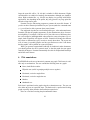
POSTMINI User’s Manual
Version 11.0-00
John Faricelli
Alpha Semiconductor Technology
Hewlett-Packard Company
Contents
1
Introduction
1
2
Functionality
1
3
Supported datafile formats
3.1 ASCII file reader . . . . . . . . . . . . . . . . . . . . . . . . . .
3.2 Plotting analytical functions . . . . . . . . . . . . . . . . . . . .
3.3 MINIMOS coordinate system and terminology . . . . . . . . . .
2
3
5
5
4
Using POSTMINI for visualization
4.1 1D plots . . . . . . . . . . . . . . .
4.2 2D contour plots . . . . . . . . . .
4.3 3D surface plots . . . . . . . . . . .
4.4 Comparison plots . . . . . . . . . .
4.5 Overlay plots . . . . . . . . . . . .
4.6 The FIND function . . . . . . . . .
4.7 The INTEGRATE function . . . . .
4.8 The LINE function . . . . . . . . .
4.9 The MINMAX function . . . . . . .
4.10 The PRINT function . . . . . . . .
4.11 Changing POSTMINI defaults . . .
4.12 The shell function . . . . . . . . . .
4.13 Managing windows on workstations
4.14 The save/restore functions . . . . .
.
.
.
.
.
.
.
.
.
.
.
.
.
.
.
.
.
.
.
.
.
.
.
.
.
.
.
.
.
.
.
.
.
.
.
.
.
.
.
.
.
.
.
.
.
.
.
.
.
.
.
.
.
.
.
.
.
.
.
.
.
.
.
.
.
.
.
.
.
.
.
.
.
.
.
.
.
.
.
.
.
.
.
.
.
.
.
.
.
.
.
.
.
.
.
.
.
.
.
.
.
.
.
.
.
.
.
.
.
.
.
.
.
.
.
.
.
.
.
.
.
.
.
.
.
.
.
.
.
.
.
.
.
.
.
.
.
.
.
.
.
.
.
.
.
.
.
.
.
.
.
.
.
.
.
.
.
.
.
.
.
.
.
.
.
.
.
.
.
.
.
.
.
.
.
.
.
.
.
.
.
.
.
.
.
.
.
.
.
.
.
.
.
.
.
.
.
.
.
.
.
.
.
.
.
.
.
.
.
.
.
.
.
.
.
.
.
.
.
.
.
.
.
.
6
7
7
10
12
14
15
15
16
17
17
18
18
18
20
5
POSTMINI printer support
21
6
Plot annotations
22
7
Expression Evaluator
23
8
POSTMINI startup file
25
9
POSTMINI command file syntax
9.1 Keyword PLOT . . . . . . .
9.2 Keyword GLOBAL . . . . .
9.3 Keyword TITLE . . . . . . .
9.4 Keyword AXIS . . . . . . .
27
31
32
33
34
.
.
.
.
.
.
.
.
i
.
.
.
.
.
.
.
.
.
.
.
.
.
.
.
.
.
.
.
.
.
.
.
.
.
.
.
.
.
.
.
.
.
.
.
.
.
.
.
.
.
.
.
.
.
.
.
.
.
.
.
.
.
.
.
.
.
.
.
.
.
.
.
.
.
.
.
.
.
.
.
.
9.5
9.6
9.7
9.8
9.9
9.10
9.11
9.12
Keyword CURVE . . . . . . . . .
Keyword CONTOUR . . . . . . .
Keyword SURFACE . . . . . . .
Keyword ANNOTATE BOX . . .
Keyword ANNOTATE LINE . . .
Keyword ANNOTATE TEXT . . .
Keyword ANNOTATE MARKER
Keyword ANNOTATE ELLIPSE .
.
.
.
.
.
.
.
.
.
.
.
.
.
.
.
.
35
39
42
44
45
46
47
48
10 Mathmode
10.1 Features . . . . . . . . . . . . . . . . . . . . . . . . . . . . . . .
10.2 Implementation details . . . . . . . . . . . . . . . . . . . . . . .
49
49
50
11 Things to look out for (bugs)
50
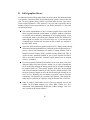
12 List of improvements and bug fixes
12.1 Improvements in version V11.0-00 .
12.2 Improvements in version V10.0-02 .
12.3 Improvements in version V10.0-000
12.4 Improvements in version V9.2-000 .
12.5 Improvements in version V9.1-000 .
12.6 Improvements in version V9.0-000 .
12.7 Improvements in version V8.3-001 .
12.8 Improvements in version V8.3-000 .
12.9 Improvements in version V8.2-001 .
12.10Improvements in version V8.1-003 .
12.11Improvements in version V8.1-001 .
12.12Improvements in version V8.1 . . .
12.13Improvements in version V8.0 . . .
12.14Improvements in version V7.4 . . .
12.15Improvements in version V7.3 . . .
12.16Improvements in version V7.2.5 . .
12.17Improvements in version V7.2.4 . .
12.18Improvements in version V7.2.3 . .
12.19Improvements in version V7.2.1 . .
12.20Improvements in version V7.2 . . .
12.21Improvements in version V7.1 . . .
12.22Improvements in version V7.0 . . .
12.23Improvements in version V6.1 . . .
ii
.
.
.
.
.
.
.
.
.
.
.
.
.
.
.
.
.
.
.
.
.
.
.
.
.
.
.
.
.
.
.
.
.
.
.
.
.
.
.
.
.
.
.
.
.
.
.
.
.
.
.
.
.
.
.
.
.
.
.
.
.
.
.
.
.
.
.
.
.
.
.
.
.
.
.
.
.
.
.
.
.
.
.
.
.
.
.
.
.
.
.
.
.
.
.
.
.
.
.
.
.
.
.
.
.
.
.
.
.
.
.
.
.
.
.
.
.
.
.
.
.
.
.
.
.
.
.
.
.
.
.
.
.
.
.
.
.
.
.
.
.
.
.
.
.
.
.
.
.
.
.
.
.
.
.
.
.
.
.
.
.
.
.
.
.
.
.
.
.
.
.
.
.
.
.
.
.
.
.
.
.
.
.
.
.
.
.
.
.
.
.
.
.
.
.
.
.
.
.
.
.
.
.
.
.
.
.
.
.
.
.
.
.
.
.
.
.
.
.
.
.
.
.
.
.
.
.
.
.
.
.
.
.
.
.
.
.
.
.
.
.
.
.
.
.
.
.
.
.
.
.
.
.
.
.
.
.
.
.
.
.
.
.
.
.
.
.
.
.
.
.
.
.
.
.
.
.
.
.
.
.
.
.
.
.
.
.
.
.
.
.
.
.
.
.
.
.
.
.
.
.
.
.
.
.
.
.
.
.
.
.
.
.
.
.
.
.
.
.
.
.
.
.
.
.
.
.
.
.
.
.
.
.
.
.
.
.
.
.
.
.
.
.
.
.
.
.
.
.
.
.
.
.
.
.
.
.
.
.
.
.
.
.
.
.
.
.
.
.
.
.
.
.
.
.
.
.
.
.
.
.
.
.
.
.
.
.
.
.
.
.
.
.
.
.
.
.
.
.
.
.
.
.
.
.
.
.
.
.
.
.
.
.
.
.
.
.
.
.
.
.
.
.
.
.
.
.
.
.
.
.
.
.
.
.
.
.
.
.
.
.
.
.
.
.
.
.
.
.
.
.
.
.
.
.
.
.
.
.
.
.
.
.
.
.
.
.
.
.
.
.
.
.
.
.
.
.
.
.
.
.
.
.
.
.
.
.
.
51
51
52
53
54
56
56
57
58
60
61
61
62
63
64
66
68
68
69
69
70
70
71
71
12.24Improvements in version V6.0 . . . . . . . . . . . . . . . . . . .
72
13 For further information and support
72
14 Acknowledgments
72
A OpenVMS Specific Notes
A.1 Setup . . . . . . . . . . . . . . . . . . . . . . . . . . . . . . . .
A.2 Command line options . . . . . . . . . . . . . . . . . . . . . . .
A.3 Floating point issues . . . . . . . . . . . . . . . . . . . . . . . .
73
73
73
74
B Unix Specific Notes
B.1 Setup . . . . . . . . . . . . . . . . . . . . . . . . . . . . . . . .
B.2 Command line options . . . . . . . . . . . . . . . . . . . . . . .
B.3 Floating point issues . . . . . . . . . . . . . . . . . . . . . . . .
75
75
76
76
C Win32 Specific Notes
C.1 Setup . . . . . . . . . . . . . . . . . . . . . . . . . . . .
C.2 Command line options . . . . . . . . . . . . . . . . . . .
C.3 Known problems with lib2d graphics library under Win32
C.4 Setup so Postmini can call Ghostscript . . . . . . . . . . .
C.5 Floating point issues . . . . . . . . . . . . . . . . . . . .
C.6 Implementation differences . . . . . . . . . . . . . . . . .
78
78
79
79
80
80
80
.
.
.
.
.
.
.
.
.
.
.
.
.
.
.
.
.
.
.
.
.
.
.
.
D Lib2d graphics library
82
E Interoperability with PC X displays
83
F Displaying Postmini graphics from a remote server to a home PC
84
G POSTMINI File Types and Default Extensions
85
H File quantity names
H.1 MINIMOS quantity names
H.2 SUPREM3 quantity names
H.3 PROMIS quantity names .
H.4 USEOUT quantity names .
H.5 VLSICAP quantity names
H.6 BAMBI quantity names . .
H.7 2DOP quantity names . . .
.
.
.
.
.
.
.
.
.
.
.
.
.
.
.
.
.
.
.
.
.
iii
.
.
.
.
.
.
.
.
.
.
.
.
.
.
.
.
.
.
.
.
.
.
.
.
.
.
.
.
.
.
.
.
.
.
.
.
.
.
.
.
.
.
.
.
.
.
.
.
.
.
.
.
.
.
.
.
.
.
.
.
.
.
.
.
.
.
.
.
.
.
.
.
.
.
.
.
.
.
.
.
.
.
.
.
.
.
.
.
.
.
.
.
.
.
.
.
.
.
.
.
.
.
.
.
.
.
.
.
.
.
.
.
.
.
.
.
.
.
.
.
.
.
.
.
.
.
87
88
89
90
91
92
93
94
H.8 PISCES quantity names . . . . . . . . . . . . . . . . . . . . . . .
H.9 SUPREM4 quantity names . . . . . . . . . . . . . . . . . . . . .
95
96
I
ASCII output file extensions
97
J
Papersizes
98
K Plot examples
99
iv
1
Introduction
POSTMINI is an interactive graphical postprocessor for device and process simulators. The postprocessor reads the save files from a number of simulation programs
(e.g. MINIMOS, MEDICI, TSUPREM4, FLOOPS, etc.) and allows the user to
examine or plot quantities stored in the file. In addition, POSTMINI can import
data from ASCII files or from analytical functions, and can be used as a general
purpose plotting program. Graphical output is available on workstations running
X11 and PostScript devices (monochrome, color and encapsulated forms) and a
variety of raster file formats. The POSTMINI command language can be used to
re-create any plot from commands in a file.
2
Functionality
The available functions in POSTMINI are:
1D - Plot an X-Y graph of 1D data, or plot a 1D cross-section of 2D data
along any vertical or horizontal line.
2D - Plot 2D contours of a quantity.
3D - Plot a quantity as a surface in 3D. These kind of plots are also known
as “bird’s eye” plots.
Compare - Plot several curves on the same graph (can be from the same or
different data files). Can also plot bar charts.
Overlay - Plot multiple contour plots on the same graph. Plots can be overlaid or offset from each other.
Find - Find where an internal quantity reaches a specified value.
Integrate - Integrate an internal quantity in a region or along a line.
Line - Print a cross-section of a 2D data along any vertical or horizontal cut
line into a file.
Minmax - Determine the minimum/maximum of an internal quantity.
Print - Print 2D data in a formatted report into a file.
Read - Read in another data file.
1
Show - List information about the simulation run (e.g. terminal voltages and
currents). Currently only for MINIMOS.
Default - Change default plot attributes of POSTMINI
Restore - Restore a plot from a Postmini command file
Shell - Execute operating commands without leaving POSTMINI.
Save - Save the current plot in a Postmini command file
Window - Manage multiple plot windows on workstations.
Exit, Quit - Terminate POSTMINI.
The quantities that can be printed/plotted depend on the simulation program.
See Appendix H for a list of internal data quantities available from each simulation
program. See Appendices A, B, and C for operating specific notes for OpenVMS,
Unix and Win32, respectively.
3
Supported datafile formats
POSTMINI can read the output file formats for a number of simulators:
ASCII data in column format
SPICE (HSPICE, DECSpice) ASCII output files (via the ASCII file reader)
SPICE3 “raw” files
DECSpice Grapes binary data files
TU Vienna MINIMOS 5.x/6.0 binary solution files (both 2D and 3D formats)
TU Vienna MINIMOS 5.x/6.0 binary doping file
TU Vienna “USEOUT” binary dump format
TU Vienna PROMIS binary data files
Univ. Florida FLOOPS/FLOODS structure files
Stanford and Univ. Texas PISCES IIB 9009 binary mesh and solution files
Stanford SUPREM-IV structure files
2
Avant! MEDICI binary mesh and solution files
Avant! TSUPREM4 ASCII structure files
Avant! TIF (TMA Interchange Format) files
Avant! HSPICE postprocessing waveform files
Vector Technologies FAIM and MCP2D files
POSTMINI can read binary files from either 2D or 3D MINIMOS runs. If
you are plotting from a 3D binary file, you will be requested for a “cut plane”
which will “slice” the device along the length, width or wafer (top view) direction.
POSTMINI supports 3D MINIMOS doping files in a similar manner.
3.1 ASCII file reader
You can also import data from an external ASCII file. The data should be arranged
in columns. Any line which begins with a “C”, “c”, “!” or “#”is taken as a comment
line. You can also use .OFF and .ON to exclude portions of a file from being read. If
you do not have enough data in a line to satisfy a read request, or have non-numeric
data on a line, that line is silently ignored. You can specify which columns are to
be read, as well as data scaling factors mx, my and ax, ay. These scaling factors
transform the data as follows:
scaled data mx input data ax
(1)
You can also specify how many lines to skip, and how many lines to read in a file.
If you have a data file which contains several data sets appended together, you can
read all the data in one step by setting the option Multiple curves in datafile
to yes. This will suppress the retrace when the X axis value goes “backwards.”
This is useful for plotting current-voltage or capacitance-voltage data files. You
can also set the “sampling” frequency, which will cause Postmini to use every
second, third, fourth, etc. point in a file. This is useful for reducing the size of
large, closely spaced, data sets, especially if symbols are also plotted. Postmini
also recognizes SPICE output files and has special support to skip automatically to
the simulation results output via .PRINT statements.
Postmini can handle ASCII files with up to 50000 data points each. If you wish
to plot different columns of data as one curve, you can specify more than Y column
or ALL to select all remaining columns.
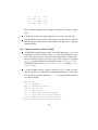
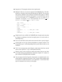
Postmini can also import ASCII files which have X-Y-Z data. The X-Y-Z format is simple way to import 2D data from an arbitrary simulator. Postmini normally
3
expects the the data to lie on a rectangular grid. The file format is similar to the
X-Y ASCII format. You may use the same commenting conventions, along with
scaling factors, including scaling the Z axis. The file format is:
x1
x2
x3
.
.
xn
x1
x2
x3
.
.
xn
.
.
.
y1
y1
y1
z
z
z
y1
y2
y2
y2
z
z
z
z
y2
z
where the x’s are the X coordinate, the y’s are the Y coordinate, and the z’s are the
function value f(x,y). Each X,Y,Z triplet must be on a single line. The (X,Y) coordinate pairs must be unique and must be specified with the X coordinate increasing
(with the Y coordinate fixed), then repeating the set of X coordinates with the next
Y coordinate value, etc.
The ASCII file reader can also read data that is not on a rectangular grid. Switch
the ”data on rectangular grid” flag in the the ”read ASCII file” menu to ”no”. In
this case, a Delaunay triangular grid is imposed on the data.
Postmini can apply general expressions to ASCII data. For example, given a
file with quantities C and E, one could plot C**2 vs. 1/E.
Postmini can also process ASCII files that have character string labels in the X
column. Character strings are delimited by blanks, tabs, equal signs or commas.
Mathmode strings may be used. To embed a blank, use the mathmode escape
;. This type of data is used to place labels under each bar on the X axis on bar
charts. Up to 200 labels may be input. The user must tell Postmini to expect X
column character data via the datafile type option in the ASCII file reader menu.
4
3.2 Plotting analytical functions
Postmini can plot analytical functions of the form y as a function of x (y f x ),
y as a function of x and an additional independent variable
p (y f x p ) or z as a
function of two independent variables x and y (z f x y ). In the first two cases,
1D data is generated. In the third case, 2D data is generated.
You can specify analytical functions by using the READ function at the main
menu (or compare submenu) and specifying an analytical “file type.”
You will be
put into a menu where you can specify the function type (e.g. f x ), the function
to be plotted, and the range of the independent variable(s). You can specify a start,
stop and step increment for each independent variable. Functions can use a variety
of mathematical expressions and math functions, see the section on the Postmini
expression evaluator for more details.
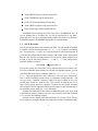
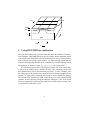
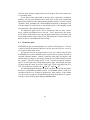
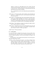
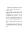
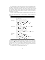
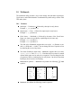
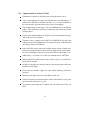
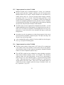
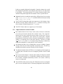
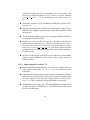
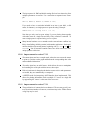
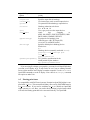
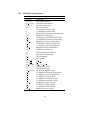
3.3 MINIMOS coordinate system and terminology
The following remarks are specific to using POSTMINI when examining MINIMOS output files. The x coordinate goes along the length direction of the FET,
from source to drain. X=0 occurs at the source end of the gate edge. The y coordinate goes along the depth direction of the FET, with y increasing with increasing
depth. Y=0 is at the oxide/silicon interface. Thus, negative y coordinates are in
the oxide; positive y coordinates are in the silicon. For binary files from 3D MINIMOS runs, you have a third (width) dimension. In the width (z) dimension, the
device extends from the middle of the channel width ( W/2) towards the field
oxide (positive). Z=0 occurs at the thin oxide mask edge in the width direction.
The following diagram illustrates the MINIMOS coordinate system.
5
Z=0
Field oxide
Z=-W/2
GATE
Y=0
Oxide
SOURCE
DRAIN
Y
Z
BULK
X=0
X=L
X
4
Using POSTMINI for visualization
After you have read in a file, you can examine the data with a number of visualization techniques. POSTMINI allows the user to visualize his/her simulation results
with contour maps (both filled color and traditional level curves), quasi-3D plots,
plots at various cross-sections in the structure, etc. After selecting a menu item, the
program will display the data that can be examined (e.g. potential, doping). Select
the quantity to be plotted, or enter 999, Q or <return> to exit this menu.
You will then be placed into a full menu screen that will allow you to make
a plot on your graphics device, annotate the plot, make a hardcopy, or alter the
plot characteristics, such as the horizontal axis limits. To alter a quantity, enter
the number next to the quantity to be modified. You will then be prompted for the
quantity. If, at this point, you decide that you don’t want to change the quantity,
enter an end-of-file (control-Z on VMS, control-D on Unix). If you enter an invalid
response, an error message will appear under the “Messages:” line. If the screen
becomes corrupted by a mail message notification or other system message, enter
R to repaint the menu on the screen.
6
4.1 1D plots
POSTMINI provides a quick way to do an X-Y plot, or plot a quantity along either
a vertical or horizontal line. POSTMINI provides the following default plot scales,
which the user can override:
The default limits for the abscissa (horizontal) axis is the entire device width/length/depth.
The default limits for the ordinate (vertical) axis is the entire data range,
rounded to “nice” numbers. Data outside the range 0.001 to 1000.0 will be
scaled by a power of ten.
You have the option of changing the default limits to plot a portion of the data or
range.
On 1D and comparison plots, you can modify the “scale factor” or remote
exponent for the plot (Note, as of Postmini V7.2, you can only modify the scale
factor for the ordinate). The scale factor is an integer power of ten that will be used
as the remote exponent in the graph. The plot data will then be scaled according to
the following relation
scaled data actual data 10scale
factor
A suggested scale factor will be displayed, this usually results in the best plotting.
A zero scale factor means no scaling will take place before plotting. Example: to
plot data with a range of 2 2 103 to 3 5 103 , you might select a data range of
2.0 to 4.0, with a scale factor of 3 (this would have been the default!).
Axis tic marks are also provided. You can specify the major tic mark increment
(real) and the frequency of minor ticmarks (integer). A major ticmark is a long tic
mark which has a number next to it. Example: a major tic mark increment of 0.1
with a minor tic frequency of 5 would plot major tics every 0.1 units, and plot a
minor tic every 0.02 units (thus dividing the major tic interval in five).
The annotation option can be used to interactively add text, lines, arrows,
boxes, symbols and elliptical arcs to the plot. Text is processed by the “mathmode” utility, which allows you to enter sub and/or superscripts, Greek letters, and
certain math symbols using a subset of the TEX math syntax. Read section 10 for
details on how to enter mathmode format strings.
4.2 2D contour plots
POSTMINI can plot a contour map (level curves) of simulation quantities over all
or a portion of the device. The user is asked to specify the portion of the device to
7
plot, and the contour values to plot. POSTMINI can plot up to 9 contours on one
graph. There are several different ways to specify contour values:
You can specify the contours by individual value, e.g.
1.0 2.0 3.0 4.0 5.0
To specify a number of contours equally spaced between a min and max
range, use the e notation:
e number-of-contours
minimum
maximum
For example, to specify 5 contours between 1 and 5:
e 5 1 5
This would result in contours at 1, 2, 3, 4 and 5.
To specify contours with a given step value, use the s notation:
s step-value
minimum
maximum
For example, to specify contours between 1 and 5 with a step of 1:
s 1 1 5
This would result in contours at 1, 2, 3, 4 and 5.
To specify a number of contours with logarithmic spacing, use the l notation:
l number-of-contours
minimum
maximum
For example, to specify 5 contours between 1014 and 1018 in logarithmic
steps:
l 5 1E14 1E18
This would result in contours at 1014 , 1015 , 1016 , 1017 , and 1018 .
To specify contours with a logarithmic step, use the d notation:
8
d step minimum
maximum
For example, to specify contours between 104 and 106 with a log step of 10:
d 10 1E4 1E6
This would result in contours at 104 , 105 , 106 . When using log steps, the
minimum and maximum have the same sign.
You can combine any or all of these notations when specifying contour values,
but you must not exceed the total number of contours.
On devices supporting many colors such as workstations, the default is to plot
contours with color fill between the contours. A different color is used to denote
different data values. This makes the contour map easier to interpret. A legend on
the side of the plot tells what values the colors represent. The first color represents
all data below the first contour value (note the “ ” before the printed value), the
second color represents all values between the first and second contour value, etc.
The last color represents all values above the maximum of the data (note the “ ”).
You may also specify tranditional contour plots using lines. Different contours
may be distinguished by different colors or by different line styles (solid, dashed,
dotted, etc.), depending on the output device. A key to the contour values is plotted
on the right side of the plot.
You can optionally plot the location of all the junctions in the structure. If you
select this option, a dashed line will be plotted at the approximate junction location.
If you request, the plot software will place small labels on each level curve so they
can be distinguished.
On workstations, you can use the mouse to intteractively zoom in on a portion
of the plot. Enter the Z (zoom) command at the menu prompt. A crosshair cursor
will appear in the plot window. Click and release the first mouse button to enter the
new lower left corner of the plot. The cursor will change to a “stretchy” box. Click
the first mouse button again to enter the new upper right corner of the plot. If you
click outside the plot area, the coordinate of the closest corner is used. Press the
second mouse button to cancel input. To return to the full coordinates, enter the U
(unzoom) command.
On workstations, you can use the mouse to interactively take a “sample” of
the contour data, and display the data value and coordinates. Enter the S (sample)
command a the menu prompt. A crosshair cursor will appear in the plot window.
Click and release the first mouse button to take a sample. The data value at that
point, plus its coordinates, will be displayed on the menu. You can continue to
9
click the mouse button to sample other areas of the plot. Press mouse button two
to exit sample mode.
If your data is better represented by discrete values, rather than a continuous
function, you can switch Postmini into a mode where it plots a box around each
data point in a different color, rather than interpolating a surface. Go to the top level
“Defaults” menu, and change the “Default hidden line method” to histogram. This
will also change 3D surface plots, so that Postmini plots a 3D histogram around
each data point, rather than interpolating a surface.
The annotation option can be used to interactively add text, lines, arrows,
boxes, symbols and elliptical arcs to the plot. Text is processed by the “mathmode” utility, which allows you to enter sub and/or superscripts, Greek letters, and
certain math symbols using a subset of the TEX math syntax. Read section 10 for
details on how to enter mathmode format strings.
4.3 3D surface plots
POSTMINI can plot an internal quantity as a surface in 3D perspective. The user
is asked to specify the portion of the device to plot; this can be used to “zoom” in
on a region of detail in the device.
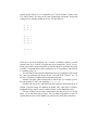
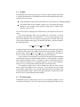
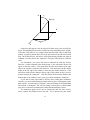
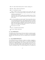
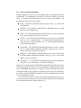
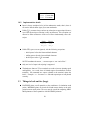
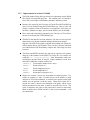
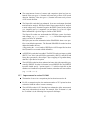
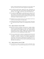
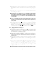
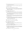
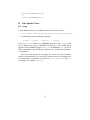
You can also move the viewing position of your “eye” relative to the 3D plot.
POSTMINI uses a polar coordinate system to specify the eye position. Position is
specified with three numbers: a radius r in microns, polar angle φ, in degrees, and
azimuth angle θ, in degrees. Increasing θ rotates the eye counter-clockwise around
the “equator.” Values for θ range from 0o to 360o . You may also specify a negative
angle; it is converted to the corresponding positive angle. Increasing φ moves the
eye down from the “north” pole to the “south” pole. Values for φ range from 0o to
180o . The default eye position is r 8 0, φ 45o , and θ 45o .
The following diagram illustrates the polar coordinate system. You may notice
that this is a left-handed coordinate system. A left-handed system is used to be
consistent with the way 3D plots are displayed by other workers. In the default
view, the source is on the left, and the drain on the right. Note that this is opposite
from the way the SURF program displays MINIMOS data.
10
φ
Z
P(r,φ,θ)
r
X
Y
θ
On devices that support color, the plot will be done using color area fill technique. This method plots the surface in different colors, depending on the “height”
of the data. This makes is very simple to determine the actual value of data being
plotted. A legend is printed on the side of the plot, similar to the 2D color contour
map. On all other devices, the surface will be plotted using a hidden line removal
technique. On color devices, the “underside” of the plot will be done in a different
color.
On workstations, you can use the mouse to intteractively rotate the 3D plot.
Enter the O (orbit) command at the menu prompt. A box around the 3D plot will
appear in the plot window. Click and release the first mouse button at the right
edge of the window to rotate the plot clockwise. Click and release the first mouse
button at the left edge of the window to rotate the plot counter-clockwise. Click
and release the first mouse button at the top edge of the window to move your eye
position towards the “north pole”. Click and release the first mouse button at the
bottom edge of the window to move your eye position towards the “south pole”.
If your data is better represented by discrete values, rather than a continuous
function, you can switch Postmini into a mode where it plots a 3D histogram, rather
than a surface. Go to the top level “Defaults” menu, and change the “Default hidden
line method” to histogram. This will also change contour plots, so that Postmini
plots boxes centered on each data point, rather than interpolating a surface.
The annotation option can be used to interactively add text, lines, arrows,
boxes, symbols and elliptical arcs to the plot. Text is processed by the “math11
mode” utility, which allows you to enter sub and/or superscripts, Greek letters, and
certain math symbols using a subset of the TEX math syntax. Read section 10 for
details on how to enter mathmode format strings.
4.4 Comparison plots
POSTMINI can plot several 1D cross-sections on the same graph. The 1D slices
can be of the same internal quantity, different quantites, or from different simulation runs. You can also import data files from different simulators, including 1D
ASCII files, for plotting.
To use this feature, select COMPARE at the main menu. You will be put into a
subsystem which has these features:
Add - Add a curve to the plot list. You will be prompted for the quantity
to plot, the cut line and coordinate (for 2D data sets). You can also specify
plot attributes such as line type (e.g. solid, dashed), color, and plotting of
symbols. A total of forty separate curves can be plotted at once.
Postmini supports multiple X and Y axes. You can associate a data curve
with either the top or bottom X axis, and the left or right Y axis. Use the
xaxis tag and yaxis tag menu items.
Barchart - Plot all the data as a bar chart.
Clear - Delete all curves from the plot list. Useful for “starting over”.
Delete - Delete a curve from the plot list.
Integrate - Integrate a quantity vertically or horizontally, and add to plot list.
This option applies to 2D data only.
List - List all curves to be plotted, with their labels.
Modify - Modify various aspects of a curve, such as the plot label, curve
color, linetype, or symbol. You can also modify the scale factors (AX, AY,
MX, MY) that were applied the data, or apply an expression to the data. You
can also select whether a curve will be included in the plot. This is useful if
you wish to store a number of data items at one time, but selectively plot the
entries. You can also change the axes the curve will be plotted on. Postmini
supports a top and bottom X axis, and a left and right Y axis.
Plot - Enter the plot menu for displaying the data as an X–Y graph.
12
Read - Read a new data file.
Show - List information about a curve
Exit, quit - Return to main menu.
The plot submenu has a variety of options for plotting:
Plot - Actually makes the plot.
Repaint - Redraws the plot menu in the terminal emulator window.
Marker - Allows the user to set a plot marker with the mouse. Two markers
are supported. Marker A is red; marker B is green. The MA command is
used to set marker A. The user can use the mouse to position a crosshair
on the graph. Pressing mouse button one will fix the crosshair and report
the marker position, and the difference (A-B). The crosshair will remain in
a fixed location on the graph as the user zooming or unzooming the graph.
The MB command works similarly for marker B.
You can also use just the M command as a shortcut. In this case, the first M
command sets marker A, and subsequent M commands sets marker B.
Grid - Turns on the plot grid. Solid lines are used at major tic marks, and
dotted lines are used at minor tic marks. The commands GX and GY can be
used to selectively turn on just the X or Y axis grid. The command GO turns
off the X or Y axis grid. Note, you must replot the graph to see any changes.
Clear - Clears the A and B markers. The commands CA and CB can be used
to selectively clear the A and B marker.
Sample - On workstations, you can use the mouse to interactively take a
“sample” of the plot, and display the X-Y coordinates. Enter the S (sample)
command at the menu prompt. A crosshair cursor will appear in the plot
window. Click and release the first mouse button to take a sample. The data
value coordinates will be displayed on the menu. You can continue to click
the mouse button to sample other areas of the plot — the change from the last
sample point is also printed. Press mouse button two to exit sample mode.
Zoom - On workstations, you can use the mouse to interactively “zoom” into
a region of the plot. Enter the Z (zoom) command at the menu prompt. A
crosshair cursor will appear in the plot window. Click and release the first
mouse button to define the lower left of the zoom area. The cursor will now
13
change to a “strechy” box, which defines the area to be zoomed. Click and
release the first mouse button to perform the zoom. Press mouse button two
to cancel the zoom. The unzoom function U will rescan all the curves and
pick bounds which will enclose all the data.
The Z2 command can be used to zoom in and make the plot bounds half their
current size.
Unzoom - Sets the plot bounds to their maximum values and replots the
graph. The U2 command can be used to zoom out and make the plot bounds
twice their current size.
Annotate - The annotation option can be used to interactively add text, lines,
arrows, boxes, symbols and elliptical arcs to the plot. Text is processed by
the “mathmode” utility, which allows you to enter sub and/or superscripts,
Greek letters, and certain math symbols using a subset of the TEX math syntax. Read section 10 for details on how to enter mathmode format strings.
Hardcopy - Enter the hardcopy submenu for creating files suitable for printing on a variety of printers (e.g. PostScript).
Keepwin - Tells Postmini to keep the current plot window on the screen, and
open a new window for the next plot. Use the Window command from the
top level menu to reactivate or delete kept windows.
Exit, Quit - Exit the plot submenu.
4.5 Overlay plots
An overlay plot consists of multiple 2D contour plots in the same window. Plots
can overlay each other, such as line contours of electron concentration over color
contours of doping concentration, or they can be spaced apart by scaling the x and
y coordinates.
To use this feature, select OVERLAY at the main menu. You will be put into a
subsystem which has these features:
Add - Add a contour plot to the plot list. You will be prompted for the
quantity to plot, if the dataset contains multiple quantities. You can also
specify plot attributes such as contour values, grid, junctions, etc. You can
also apply scaling or expressions to the x and y coordinates and the data
itself. A total of forty separate contour plots can be plotted at once.
14
Clear - Delete all data from the plot list. Useful for “starting over”.
Delete - Delete a dataset from the plot list.
List - List all data to be plotted.
Modify - Modify various aspects of a dataset, such as contour values, grid,
junctions, etc. You can also apply scaling or expressions to the x and y
coordinates and the data itself.
You can also select whether a dataset will be included in the plot. This is
useful if you wish to store a number of data items at one time, but selectively
plot the entries.
Plot - Plot all the data as an contour graph. The plot menu allows the user
to set certain global plot attributes, such as applying a global set of contours
to be used with all datasets, and setting the dataset that will be used for the
sample function and also for plotting the contour map legend at the side of
the plot. The other functions available for contour plots (e.g. zoom, unzoom,
sample, save) are available for overlay plots.
Read - Read a new data file.
Show - List information about a dataset
Exit, quit - Return to main menu.
4.6 The FIND function
The FIND function will search along a 1D cut line in the device and print out where
a simulation quantity reaches a certain value. For example, you can use FIND to
determine where the lateral electric field is zero along the surface of the MOSFET
(Y=0).
4.7 The INTEGRATE function
The INTEGRATE function will integrate a quantity in an arbitrary rectangular region in the device, or along a 1D cut line in the X, Y or Z direction. INTEGRATE
prompts for the region to integrate, and will check to make sure the region is inside the device. INTEGRATE prints out certain landmarks in the device, such as
the source and drain contact positions, and the gate position, for the user’s convenience in specifing the region. Note that the integration area is rounded to the
15
nearest simulation mesh line, so integration over exact regions is not possible in
general. In most cases, there are sufficient mesh lines to resolve the use specified
integration region. As a check, POSTMINI will print out the actual integration
region for the user to check. Also note that the resulting integrated value is given
per centimeter (cm) device width (or length/depth, if 3D data is being integrated).
Integration over a line can be thought of as integrating over a plane that is
inserted perpendicularly to the simulated device (in the z, or width direction, for
example). When performing a line integration of a vector quantity, such as current density or electric field, the vector component perpendicular to the cut line is
usually chosen. For example, if the cut line is in the vertical (Y) direction, the integral of the x component of the current density gives the amount of current flowing
though across that line. One should be cautious when integrating the y component
of the electric field at the oxide interface since field is discontinuous at that point.
POSTMINI computes the electric field at the semiconductor side of the interface
and uses the result at that point.
POSTMINI also allows you to perform a 1D integration of any 1D data that
has been loaded, e.g. from an ASCII file, etc.
Note well: integrating over an area with the same X or Y coordinate is not the
same as integrating over a line. Quantities integrated over a region are weighted
by area (cm2 ), while those integrated over a line are weighted by length (cm).
POSTMINI prints the units of the integrated quantity to remind the user.
Note well: the integration method does not take nonplanar boundaries correctly
into account (uses entire area weight, rather than area in just silicon). Use caution
when integrating near nonplanar features.
Example 1: Integrate the avalanche generation over the entire device. Multiply
this number by the electronic charge q to get the bulk current per cm of device
width. Note: this number can be different from what MINIMOS prints, especially
when the bulk current is very small compared to the drain current.
Example 2: Integrate the X component of the minority current in a vertical
direction in the middle of the channel. This gives the drain current per cm width
of the device. Note, if MODEL=AVAL or HOT, there may be a slight difference
between this current and the drain current printed by MINIMOS, due to additional
current generated by impact ionization. By varing the length of the integration line,
one can determine the amount of current that passes a certain depth.
4.8 The LINE function
Using the LINE function, you can print simulation internal quantities along any
vertical or horizontal line. The first lines of the file are a header which lists the
16
quantity and cut line selected. This header is commented out using the CURV
program convention, so these files can be directly read by CURV. Following the
header, the data is printed out in two columns: the coordinate (in microns) and the
quantity at that coordinate.
When you print data into a file, POSTMINI creates a file in your current directory, using the following algorithm to generate the file name:
1. The stem of the binary file name is the first part of the print file. Example:
binary file is GEN505000.BIN; stem is GEN505000.
2. The coordinate of the cut is appended to the file name in the format nnnnC,
where nnnn is the absolute value of the cut coordinate value in 1000’ths of
microns, and C is the cut direction (X or Y). Examples: cut at X = 1.25
1250X; cut at Y = 0 050 microns 0050Y.
microns 3. The file type is a mnemonic code which depends on the quantity selected.
See section 8dix B for the list of extensions and their meaning.
4.9 The MINMAX function
The MINMAX function allows you to locate the minimum and maximum of a
quantity in the simulation. Note that it is possible that there will be several places
in the device which have the same minimum or maximum value. POSTMINI will
report the first one it finds as it scans the device. You can limit the seach to a portion
of the device; this is useful if you wish to limit seaching to the semiconductor
region (e.g. y 0 in a planar MOSFET).
4.10 The PRINT function
Using the PRINT function, you can print simulation internal quantities over the
entire device to a file. Output consists of a neatly printed array of data values, with
corresponding x and y coordinates.
When you print data into a file, POSTMINI creates a file in your current directory, using the following algorithm to generate the file name:
1. The stem of the binary file name is the first part of the print file. Example:
binary file is GEN505000.BIN; stem is GEN505000.
2. The file type is a mnemonic code which depends on the quantity selected.
See section 8 for the list of extensions and their meaning.
17
4.11 Changing POSTMINI defaults
POSTMINI allows you to change a number of default plot attributes. Use the
default function to modify them. The following attributes can be modified from
within Postmini:
Attribute
Force solid lines on contour plots
Linewidth scale factor
Hidden line algorithm
Default hardcopy device
Workstation window size factor
Hardcopy reduction factor
Hardcopy orientation
Text scale factor
Force autoscale of coordinate axes
Length unit name
Possible values
Yes/No
0.0 – 5.0
Device dependent
Horizon function
Painter’s algorithm
(See list of supported devices)
0.1 factor 1.0
the factor is a percent of
the full workstation screen
0.1 factor 1.0
Landscape/Portrait
1.0 enlarges all text
1.0 shrinks
Yes/No
Arbitrary string
4.12 The shell function
You can execute operating system commands without leaving POSTMINI by using
the shell function. Under VMS, your DCL prompt will be set to Postmini>, to
remind you that you must return to POSTMINI (type LOGOUT to do this). Under
Tru64 Unix, a C-shell process is created. Type “exit” or “control-D” to return to
POSTMINI.
4.13 Managing windows on workstations
When POSTMINI is run on a workstation, it can plot data in multiple windows.
Select the “windows” option from the main menu. From there, you can opt to delete
any or all plot windows on the screen, or select the “style” of window management.
The three available styles are:
Single window - All plots go to a single window.
18
Multiple - Each plot type (e.g. 1D, contour, 3D, comparison) uses a separate
window.
Reactivate - Reactivate plot windows that have been “saved” on the screen.
Retained - All plots go to a single window; however, you can elect to save
the current window on screen. POSTMINI will prompt you when the plot
is completed if you want to save the window. POSTMINI will open a new
window for the next plot. Retained windows remain on the screen until you
delete them. You may keep up to 10 windows on the screen at once.
The default style is “retained”.
If you use several windows, you will probably want to rearrange or shrink/expand
the windows to your liking. Use the normal Motif window manager functions to
manipulate the GKS plot window. Under Motif, when a window is re-sized, the underlying graphics are redrawn to fit in the window, while maintaining the original
aspect ratio of the plot.
Under Motif, you may notice that the window “input focus” is transferred to
the GKS window whenever there in any input or output to that window. This
is inconvenient when using Postmini, since you need to click on your terminal
window to restore input focus so you can type at the terminal window. This also
has the side effect of popping the terminal window up so that it covers the graphics
output. This is especially annoying when performing graph annotations. One way
to avoid this problem is to change the Motif window manager input focus policy
so that input focus is assigned to the window where the mouse is pointing. To do
this, click and hold down mouse button 1 on any part of the background window. A
menu should come up. Point to “Options ” and select the “Workspace” submenu.
Under “To make a window active”, select the “Move the pointer into the window”
option. Also, turn off the option “Raise it to the top of the screen” under “When
a window becomes active.” Then save the settings and restart the Motif window
manager.
If you do not like the “focus follows mouse” approach, you can just turn off
the option “Raise it to the top of the screen” and restart the Motif window manager. When the Postmini graphic window comes up, focus will be on the graphics
window, but you can move it back to the terminal string by clicking anywhere
on the terminal window. Click on the window border to raise the window to the
foreground.
19
4.14 The save/restore functions
Postmini supports the option to save a description of the current plot in a Postmini
command file. The command file is ASCII text, and can be edited with any text
editor. It contains all the information necessary to re-plot your graphics. The
command file consists of several sections:
PLOT – The PLOT command describes the type of plot – e.g. 1D, 2D, 3D
or COMPARE.
GLOBAL – The GLOBAL command and its subsequent lines set overall
factors, such as defining colors
AXIS – The AXIS command defines the limits on the various axis parameters, such as minimum, maximum, tic marks, etc.
CURVE – The CURVE command defines the how to restore an individual
curve of a 1d or comparison plot. It contains datafile information (filename, data type, cut line coordinate, etc.) as well as plotting information
(color/marker information).
CONTOUR – The CONTOUR command defines how to restore a contour
plot. It contains datafile information (filename, data type, etc) as well as
contour values used, and other plot options.
SURFACE – The SURFACE command defines how to restore a surface plot.
It contains datafile information (filename, data type, etc) as well as other
options, such as eye position.
ANNOTATE – The ANNOTATE command defines the various annotations
of the plot – boxes, lines/arrows, text, markers and ellipses.
In general, you would generate a POSTMINI command file using the save function.
It is entirely possible to generate one yourself, although it would probably be better
to use a POSTMINI generated file as a template. The restore function attempts to
catch invalid input as best as possible, and reports syntax errors to the terminal by
line number of the POSTMINI command file. Section sec:pmifile lists the current
set of command file keywords.
Once you restore a plot, you will be placed into an appropriate full screen, e.g.
if you restored a 2D contour plot, you will be placed in the 2D contour plot menu.
You can then plot, annotate, make a hardcopy, etc.
20
Note that POSTMINI when restores a plot, it re-reads the original datafiles. If
the datafiles have been deleted, modified or are in another directory, then POSTMINI may not be able to restore the plot, or a unexpected graph may be displayed.
POSTMINI automatically saves your last plot in a file called POSTMINI.PMI
when you exit the program. Under VMS, a new version of the file is created, so
you should occasionally purge the POSTMINI.PMI files.
5
POSTMINI printer support
If you want to make a hardcopy plot file, select the Hardcopy menu option. Another full screen menu will come up. To generate a hardcopy, enter P. To return
to the previous menu without making a hardcopy, enter Q or E. You may make a
hardcopy without previewing the graph on your screen. Note: POSTMINI will
only create the plot file; it is up to you to print the file.
POSTMINI supports a number of output devices. Under lib2d graphics, the
supported devices are: color and monochrome PostScript, encapsulated PostScript
(for inclusion in other documents, like Microsoft Word or LaTeX), Portable Network Graphics (PNG) raster files, Portable PixMap (PPM) raster files, Raw (binary) PPM files and Tagged Image File Format (TIFF) raster files. The plot file
will have the name corresponding to the data file you read in, with an extension
depending on the type of hardcopy, e.g. .ps for PostScript.
Supported Hardcopy Devices (Lib2d graphics)
Hardcopy device
Default
extension
Postscript
.ps
Color Postscript
.ps
Encapsulated Postscript
.eps
Color Encapsulated Postscript .eps
PNG
.png
PPM
.ppm
PPMRAW
.ppmraw
TIFF
.tiff
You may specify a different output file name from the hardcopy menu. The PNG
format is highly recommended as it generates highly compact files and with good
fidelity. PNG files are supported for import and display by the Microsoft Office 97
and 2000 suites, Internet Explorer and Netscape. For raster file formats, one can
specify the raster resolution, in pixels per inch (dpi). The higher the resolution, the
21
larger the raster file will be. 50–100 dpi is suitable for Web documents. Higher
resolution files are suitable for hardcopy documentation, although care should be
taken. High resolution files, e.g. 300 dpi, may display very quickly in MS Office
applications, but depending on the printer, they may generate very large print files
and take a long time to print.
Postmini uses the Ghostscript program to generate the raster file formats. If
you do not have Ghostscript installed on your system (under the command name
gs), you will not be able to generate these raster formats.
One might ask why there are two PostScript file types: color and monochrome.
Postmini will alter the graphics appearance for the monochrome device for maximum legibility. For example, if one has an X-Y plot with curves of different colors,
the curves might be indistinguishable when printed to a non-color printer. For example, both red and blue will appear as black. Postmini will change the different
line colors to different line types, in order to clearly show them. The expert user
will, of course, just modify graph to use line types and not use color if s/he knows
that the graphic will be printed on a non-color printer.
When you generate encapsulated PostScript for inclusion in other documents,
you should generate the file in portrait mode, so that the graph does not appear
rotated by 90 degrees. Postmini automatically does this for encapsulated PostScript
and all the raster formats.
6
Plot annotations
POSTMINI allows the user to interatively annotate any graph. This feature is available only on workstations. The user can add the following items to a graph:
Boxes, both filled or outline
Elliptical arcs (useful in grouping multiple curves together)
Horizontal, vertical or angled lines
Horizontal, vertical or angled arrows
Markers
Mathmode text
Each item is positioned on the graph using the workstation mouse. The user can
also delete any item, or reposition items. The final result is a professional looking
graph, especially when plotted to the PostScript output device.
Here are a few hints on using the plot annotation feature:
22
When you ask to draw a vertical or horizontal line, POSTMINI will “snap”
the line to the vertical or horizontal, even if you try to draw a line that is at
an angle.
Filled boxes drawn using a color of “0” (background color) can be used to
block out portions of the plot (like electronic “white–out”). This is especially
useful in placing text in colored or busy areas of a plot. First draw a filled
box the size of the text, then place the text over the box.
Elliptical arcs are drawn in two steps (v8.2 and higher). First, the user clicks
on the lower left and upper right corners of a rectangle that is the bounding
box for the arc. Postmini then displays an elliptical arc in “real time.” The
end points of the arc change as the user moves the mouse. Clicking on mouse
button one finishes the process.
Under some conditions, it is possible for an elliptic arc to “cover” another
item, so that the underlying item cannot be selected for deletion or re-positioning.
To uncover the item, move the elliptic arc off the item you wish to select.
POSTMINI uses the built-in PostScript fonts (default: Helvetica Bold) when
plotting to the PostScript device. These fonts are professional quality, and
are highly legible, even after photo-reduction. The down side of using these
fonts is that they are not exactly the same as the fonts used on the workstation. Although the fonts are all scaled to the same size, it is possible that text
may come out slightly different in size on these two devices. The difference
is usually negligible. The other hardcopy devices do not have this problem.
You can use horizontal or vertical line annotations to “measure” distances.
For example, to measure the horizontal distance from the edge of a MOSFET
gate to the junction edge, enter a horizontal line with one end on the gate
and the other on the junction edge (remember, horizontal lines “snap” to
horizontal, so you enter an angled line if that’s more convenient). Then move
the horizontal line down to the horizontal plot axis to determine its length.
7
Expression Evaluator
Postmini has a very general expression evaluator code. This allows the user to
apply arbitrary expressions to their X or Y axis data, either when read in from an
ASCII file, or in a comparison plot. Expressions use a syntax similar to Fortran.
The common arithmetic operators +, -, *, / and ** (exponentiation) are supported,
23
along with comparison operators ( , , , , ), binary and (&), binary or
(|), logical and (&&), logical or (||), parenthesis to group operations, as well as a
number of functions listed below.
function
name
sqrt
log
exp
log10
abs
sin
cos
tan
asin
acos
atan
atan2
Operation
sqrt
log base e
exponential function
log base 10
absolute value
sine function (radian argument)
cosine function (radian argument)
tangent function (radian argument)
arcsin function (returns radians)
arccos function (returns radians)
arctan function (returns radians)
arctan function with two arguments (returns
radians)
max(...)
maximum function (arb. number of arguments)
min(...)
minimum function (arb. number of arguments)
sind
sine function (degree argument)
cosd
cosine function (degree argument)
tand
tangent function (degree argument)
sinh
hyperbolic sine function
cosh
hyperbolic cosine function
tanh
hyperbolic tangent function
ran
random function [0,1.0], takes one (dummy)
argument
merge(a,b,c) if c is true, then a, else b
The following functions are valid for 1-D data
integrate(y,x) Integrate y(x) from initial x to current x value
deriv(y,x)
Differentiate y with respect to x
select(a,t)
if t is true, then return expression a
Note that only one differentiate function is allowed per expression. Versions
9.1-002 and higher of Postmini implement a two-pass function evaluator, which
allows implementation of a central difference differentiator, which is more numerically accurate than in previous versions.
24
When applying expressions to simulator data, a single variable is allowed, either x, y or z, which refers to the X, Y or Z data which will be transformed.
When applying expressions to ASCII data, the situation is more complicated. If
only one X and Y column have been loaded, then the variables x or y are permitted
in either the X or Y expression. If multiple Y columns have been loaded, then the
“y” variables are named after the columns in which they appeared in the original
file. For example, if you loaded columns 2 and 3 as Y columns, then the y variable
names you could use in an expression are y2 and y3.
The merge function can be used to implement an if-then-else construct.
For example, one could specify the Y expression as merge(y,0,y>0). Where y
was greater than zero, its value would be plotted, otherwise zero would be plotted.
The select function can be used to select a subset of the data to be plotted.
For example, one could specify the Y expression as select(y, x>0). This would
plot only data where the x variable was greater than zero. More complicated tests
can be constructed from simpler tests combined with logical and and or.
The ran function can be used to provide a sequence of random numbers. Due
to a limitation in the expression parser, a single argument must be supplied to the
ran function. Its value is ignored.
If an expression is used, any linear scaling factors (AX,AY,MX,MY) are not applied.
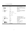
8
POSTMINI startup file
When POSTMINI starts up, it reads a file named POSTMINI DEFAULTS.DAT from
your current directory. If no such file exists, it tried to read it from your home
directory. The startup file can be used to modify many features of Postmini. The
file consists of lines as follows:
keyword =
[value1 [[value2] ...]
Keywords are case independent. Blanks or commas may be used to separate values.
Comment lines begin with an exclamation point “!” in column 1. You may place
several items on one line by separating the items with a semicolon. The following
is a sample startup file:
!
!
!
!
A sample Postmini default file
Make hardcopy in portrait orientation
25
hc_orientation = portrait
! Define default 3D view at radius=8, phi=45 degrees,
! theta=45 degrees
3d_view = 8 45 45
! Use Courier font
default_font = courier
! Redefine color #2 as light gray
color_2 = 0.7 0.7 0.7
The following table lists all valid keywords for the Postmini startup file POSTMINI DEFAULTS.DAT.
In the following table, string means any string, int means any integer, and
real means any real number. String values are taken from the first non-blank
character after the equal sign to the last non-blank character of the line. The following keywords are recognized:
Postmini default file keywords
Key
Values
3D VIEW
real real real AUTOSCALE
YES | NO
COLOR nn
real real real – or –
HARDCOPY
string postscript | eps
| color postscript | color eps
| png | tiff | ppm | ppmraw
portrait | landscape
HC ORIENTATION
26
Description
Default 3D viewpoint (radius, phi, theta)
If “YES”, always generate new default plot axis
limits using an autoscaling algorithm
If “NO”, remember the last coordinate axis limits the user specified and use for the next plot
(default)
Defines red/green/blue components of color nn nn
ranges from 0 to 15. Postmini normally uses colors 0–11.
Color 0 specifies the background color
Name of color nn
Default hardcopy device
Hardcopy orientation
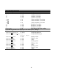
Postmini default file keywords (cont)
Key
Values
HIDDEN LINE METHOD
painter — horizon
LENGTH UNIT NAME
string real AND SCALE
YES | NO
OXIDE FILL
PLOT SCALE FACTOR
DEFAULT FONT
real (0.1 to 10.0)
string LINEWIDTH SCALE
SOLID CONTOUR LINES
TEXT SCALE
WRITE PMIFILE
real No value
real (0.1 to 10.0)
YES | NO
Z COLORMAP MINIMUM
Z COLORMAP MAXIMUM
real real 9
Description
3D hidden line method
Name of length unit and scale to cm
Fill regions of oxide with background color if oxide does not have any data associated with it
For debugging only, default: YES
Plot reduction/enlargement factor
Selects text font to use for Postscript plots (see
section 9)
Linewidth scale factor
Makes all 2D contour lines solid
Text reduction/enlargement factor
If YES, writes .PMI file at end of Postmini run
(default: YES)
Value of colormap minimum for 3D plots
Value of colormap maximum for 3D plots
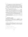
POSTMINI command file syntax
The Postmini command file describes all the data needed to recreate a Postmini
plot from the original data files. The command file breaks a Postmini plot into
several parts, such as type of plot, axis description, data source, annotations, etc.
In order to use the same code as for reading the Postmini defaults file, the Postmini
command file uses a similar general syntax: a keyword, an (optional) equal sign,
and an (optional) list of arguments. Certain special keywords called main keywords
introduce each part of the plot, and tell Postmini what to expect next. Each main
keyword is followed by subkeys which give further information.
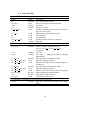
The following table lists all valid main keywords for the Postmini command
file. Note that some keys go together; for example, a file with a PLOT 2D key
must have a CONTOUR key. Keywords may be in any case. They must be spelled
out completely. Comments are started by an exclamation point ! in column 1.
A choice is denoted by the syntax word1 | word2 | .... Note that new main
keywords may be added in later versions of Postmini.
27
Key
PLOT
CURVE
Values
1D | 2D | 3D |
COMPARE | BARCHART
OVERLAY
none
string X | Y | Z
(optional)
BOTTOM | TOP |
LEFT | RIGHT
none
CONTOUR
none
SURFACE
ANNOTATE
none
LINE | BOX | TEXT |
MARKER | ELLIPSE
GLOBAL
TITLE
AXIS
Description
Type of plot
Global plot parameters
Titling to appear at top of plot
Axis parameters
Source of data for a 1D or COMPARE plot.
There can be multiple CURVE commands in a
COMPARE plot
Source of data for a 2D contour plot
There can be multiple CONTOUR commands in an
OVERLAY plot
Source of data for a 3D surface plot
Data for an annotation
28
The subkeywords for each main keyword are listed in the following tables.
Note that new subkeywords may be added in later versions of Postmini. In the following table, string means any string, int means any integer, and real means
any real number. String values are taken from the first non-blank character after
the equal sign to the last non-blank character of the line. Quoting is not needed to
maintain the case of strings.
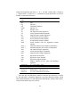
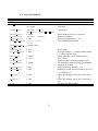
Postmini 7.4-000 and higher supports symbolic names for colors, line types,
marker types and PostScript fonts, as well as integers. Postmini recognizes the
following:
Item
Color
Line types
Marker types
PostScript
fonts
Values
Dependent on plot type
See tables below
Also: invisible, off, none
solid, dashed, dotted, dash dot
dash 2 dot dash 3 dot long dash
long short dash spaced dash spaced dot
double dot triple dot
none off omit
circle, square, triangle up, triangle down
solid circle, solid square
solid tri up, solid tri down
dot, plus, asterisk, cross
bowtie, hourglass, diamond
solid bowtie, solid hourglass, solid diamond
none off omit
times, times italic
times bold, times bold italic
helvetica, helvetica oblique
helvetica bold, helvetica bold oblique
courier, courier olblique
courier bold, courier bold oblique
You can still use integers to specify these items, if you wish. Note well! If you have
used the COLOR NN command to change Postmini’s default colors, the color name
associated with index NN will no longer be recognized by Postmini. In its place,
the name userdefinednn will be recognized. The color names are taken from the
list of X11 colors (on Unix, see: /usr/lib/X11/rgb.txt).
The default colors for 1D and comparison plots are:
29
Color Index
0
1
2
3
4
5
6
7
8
9
10
11
12
13
14
15
Name
white
black
red
green
blue
cyan
magenta
yellow
lightgreen
gold
lightblue
orange
purple
brown
gray
violet
The default colors for 2D and 3D plots are:
Color Index
0
1
2
3
4
5
6
7
8
9
10
11
12
13
14
15
Name
white
black
purple
blue
deepskyblue
cyan
green3
green
yellow
gold
orange
red
undefined1
undefined2
undefined3
undefined4
30
9.1 Keyword PLOT
Keyword PLOT
Subkey
Values
Description
Does not have any subkeys at this time.
31
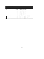
9.2 Keyword GLOBAL
Keyword GLOBAL
Subkey
COLOR nn
COLORMAP TYPE
HARDCOPY DEVICE
HC ORIENTATION
HC SCALE FACTOR
HIDDEN LINE METHOD
LENGTH UNIT NAME
AND SCALE
LINEWIDTH SCALE
PLOT SCALE FACTOR
Values
real real real or string SPECTRUM | RED BLUE
GRAY SCALE | INVERTED GRAY SCALE
string LANDSCAPE | PORTRAIT
real device | painter |
horizon
string real Description
Red,green,blue components of color
color name
colormap type
real real Scales all lines
Scales plot window, 1.0 makes window smaller,
1.0 makes window larger
Default font name (see list of names above)
Scales all text
Suppresses labels at bottom of compare plots
Two chararacters used as left and right delimiters
around the units string
Scales the hardcopy plot (0.1 1.0)
Modifies the aspect ratio of the hardcopy plot (0.1
2.0, default=0.77)
Offsets the hardcopy plot in the X direction ( 1.0)
Offsets the hardcopy plot in the Y direction ( 1.0)
Sets raster plot file resolution
DEFAULT FONT
TEXT SCALE
SUPPRESS LABELS
UNIT DELIMITERS
string real HC SCALE FACTOR
HC ASPECT RATIO
real real HC XOFFSET
real HC YOFFSET
real HC DPI
real string 32
Default hardcopy device (see section 8)
Hardcopy orientation
Hardcopy reduction factor, 1.0
Type of hidden line algorithm
9.3 Keyword TITLE
Keyword TITLE
Subkey
string Values
Description
Does not have any subkeys at this time.
The TITLE command is used to put text labels at the top of plots. For 1D, 2D, 3D
plots, only one title line can be specified. For comparison plots, up to five title
lines can be specified. For overlay plots, up to three title lines can be specified. If
you use more than two titles, you should also specify either SUPPRESS LABELS or
CURV MODE on the GLOBAL command to make more room on the plot for titling.
33
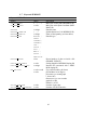
9.4 Keyword AXIS
Keyword AXIS
Subkey
ABS
EXPONENT
LABEL
LOG
LOG TIC FREQ
Values
No value
int string No value
int Description
Take absolute value of data
Power of 10 used to scale (divide) data
Axis label
Take log10 of data
Number of decades between major tic marks on
log scale (Z axis only)
MAJOR TIC
real Major ticmarks placed at this interval
MAX
Axis maximum
real real MIN
Axis minimum
MINOR TIC FREQ
Number of minor ticmarks per major tic
real string UNITS
Data units
The following are supported for comparison plots only
AUTOSCALE
No value Choose min/max, depending on data
MIN,MAX,MAJOR TIC,MINOR TIC FREQ
are ignored.
COLOR
Axis color
string string FORMAT
Any value “C” language format for a floating
point number
MAJOR GRID
No value Plot a grid line at each major tic mark
MAJOR GRID LINETYPE int Linetype for major grid lines
MAJOR TIC FACTOR
Major tic scale factor (ratio of length of major tic
real to minor tic)
MINOR GRID
No value Plot a grid line at each minor tic mark
MINOR GRID LINETYPE int Linetype for minor grid lines
real MINOR TIC SIZE
Minor tic scale factor (in percent of entire graph)
NONUMBERING
No value Omits numbering at major tic marks
OMIT
No value Do not draw in the axis at all
THICKNESS
Axis thickness scale factor
real The following are supported for contour and overlay plots only
INVERT
No value Draw the Y axis with increasing values going
down
34
9.5 Keyword CURVE
Keyword CURVE
Subkey
ALONG OXIDE
AX
AY
COLOR
CUT LINE AXIS
CUT LINE COORD
CUT PLANE AXIS
CUT PLANE COORD
Values
No value
real real string X | Y | Z
real X | Y | Z
real DATAFILE RECORD
string 1 | 2 | 3
string MINIMOS | PROMIS |
SUPREM3S | SUPREM3P |
2DOP | USEOUT |
SUPREM4 | PISCES | UTPISCES
ASCII | TIF | GRAPES |
SPICE3 | HSPICE | FAIM | MCP2D |
MEDICI | FLOOPS
ANALYTICAL
int DOPFILE GATE LENGTH
DOPFILE INTERFACE FILE
real string INTEGRATED
INTEGRATION DIRECTION
X | Y | Z
DATAFILE
DATAFILE DIMENSION
DATAFILE QUANTITY
DATAFILE TYPE
35
Description
Make cutline along oxide interface
Added to X axis data
Added to Y axis data
Color of curve
Make cutline along this axis
Make cutline at this coordinate
Make cutline on this plane (MINIMOS 3D)
Make cutline at this plane coordinate (MINIMOS
3D)
Data file name
Spatial dimension (3 for MINIMOS 3D)
Name of data quantity (see later tables)
Data file type
Record number of data set inside a file
(PROMIS, USEOUT)
Scaling length for MINIMOS doping file
Interface file associated with a MINIMOS doping
file
Quantity is integrated
Direction to integrate
Keyword CURVE (cont)
Subkey
LABEL
LINETYPE
LINEWIDTH
MARKER COLOR
MARKER SIZE
MARKER TYPE
MX
MY
SORT
XABS
XAXIS TAG
Values
string string real string real string real real No value
No value
TOP | BOTTOM
X EXPRESSION
YABS
YAXIS TAG
string No value
LEFT | RIGHT
Y EXPRESSION
VLSICAP GATE EDGE
VLSICAP SI SIO2 INTERFACE
string real real Description
Text string
Line types (see list above)
Linewidth (1.0 == default)
Marker color
Marker size (1.0 == default)
Postmini marker type (see list above)
Multiplies X axis data
Multiplies Y axis data
Sorts data on X coordinate before plotting
Takes absolute value of X coordinate
Associates this curve with the
top or bottom axis
(comparison plots only)
Expression to apply to X axis data
Takes absolute value of Y coordinate
Associates this curve with the
left or right axis
(comparison plots only)
Expression to apply to Y axis data
Position of gate edge
Position of Si/SiO2 interface
36
Keyword CURVE (cont)
The following parameters are valid only for the ASCII datatype
Subkey
Values
Description
AZ
Adds to Z coordinate
real CHARACTER DATA IN X COL No value Labels for barcharts
COL X
int Column which has X axis data
COL Y
Column(s) which have Y axis data
int – or –
ALL
All remaining columns
COL Z
Column which has Z axis data
int ERRORBARS
Plot error bars using Z column data
MZ
Multiplies Z coordinate
real int READ LINES
Read only n lines in file
SAMPLE FREQ
int Read every int lines
SKIP LINES
Skip n lines in file before reading
int SWEEP
No value Suppress retrace if X axis data is
non-monotonic
ZABS
No value Takes absolute value of Z coordinate
ZSORT
No value Sorts data on Z coordinate before plotting
The following parameters are valid only for the GRAPES datatype
Subkey
Values
Description
GRAPES XAXIS QUANTITY
Quantity to plot along X axis
USE GRAPES DICTIONARY
No value Use dictionary information to translate between
netlist names and SPICE internal names/node
numbers.
The following parameters are valid only for the SPICE3 datatype
Subkey
Values
Description
SPICE3 XAXIS QUANTITY
Quantity to plot along X axis
The following parameters are valid only for the HSPICE datatype
Subkey
Values
Description
HSPICE XAXIS QUANTITY
Quantity to plot along X axis
37
Keyword CURVE (cont)
The following parameters are valid only for the ANALYTICAL datatype
Subkey
Values
Description
ANALYTICAL EXPRESSION
Analytical expression
string ANALYTICAL FUNCTION TYPE F(X) |
Analytical function type
F(X,P) | F(X,Y)
real ANALYTICAL XSTART
Starting x value
ANALYTICAL XEND
real Ending x value
ANALYTICAL XSTEP
X step
real real ANALYTICAL PSTART
Starting p value
ANALYTICAL PEND
Ending p value
real real ANALYTICAL PSTEP
P step
ANALYTICAL YSTART
real Starting y value
ANALYTICAL YEND
Ending y value
real real ANALYTICAL YSTEP
Y step
38
9.6 Keyword CONTOUR
Keyword CONTOUR
Subkey
COLOR
CUT PLANE AXIS
CUT PLANE COORD
Values
No value
X | Y | Z
real DATAFILE RECORD
string 2 | 3
string MINIMOS | PROMIS
SUPREM3S | SUPREM3P |
2DOP | USEOUT |
SUPREM4 | PISCES | UTPISCES
ASCII | TIF |
FAIM | MCP2D |
MEDICI | FLOOPS
ANALYTICAL
int DOPFILE GATE LENGTH
DOPFILE INTERFACE FILE
real string JUNCTIONS
GRID
NEGATE
VLSICAP GATE EDGE
VLSICAP SI SIO2 INTERFACE
VALUES
No value
No value
No value
real real real real ...
(up to 9 values)
DATAFILE
DATAFILE DIMENSION
DATAFILE QUANTITY
DATAFILE TYPE
39
Description
Enables color fill contour
Make plot on this plane (MINIMOS 3D)
Make plot at this plane coordinate (MINIMOS 3D)
Data file name
Spatial dimension (3 for MINIMOS 3D)
Name of data quantity (see later tables)
Data file type
Record number of data set inside
a file (PROMIS, USEOUT)
Scaling length for MINIMOS doping file
Interface file associated with a MINIMOS doping file
Plots junctions
Plots grid
Negates data before plotting
Position of gate edge
Position of Si/SiO2 interface
Contour values
Keyword CONTOUR (cont)
The following parameters are valid only for the ASCII datatype
Subkey
Values
Description
AX
Added to X axis data
real real AY
Added to Y axis data
AZ
Added to Z axis data
real int COL X
Column which has X axis data
COL Y
int Column which has Y axis data
COL Z
Column which has Z axis data
int real MX
Multiplies X axis data
MY
Multiplies Y axis data
real real MZ
Multiplies Z axis data
SKIP LINES
int Skip n lines in file before reading
The following parameters are valid only for the ANALYTICAL datatype
Subkey
Values
Description
string ANALYTICAL EXPRESSION
Analytical expression
ANALYTICAL FUNCTION TYPE F(X) |
Analytical function type
F(X,P) | F(X,Y)
real ANALYTICAL XSTART
Starting x value
ANALYTICAL XEND
Ending x value
real real ANALYTICAL XSTEP
X step
ANALYTICAL PSTART
Starting p value
real real ANALYTICAL PEND
Ending p value
ANALYTICAL PSTEP
real P step
ANALYTICAL YSTART
Starting y value
real real ANALYTICAL YEND
Ending y value
ANALYTICAL YSTEP
Y step
real 40
Keyword CONTOUR (cont)
The following parameters are may be used for any datatype in OVERLAY plots
Subkey
Values
Description
AX
Added to X axis data
real real AY
Added to Y axis data
AZ
real Added to Z data
MX
Multiplies X axis data
real real MY
Multiplies Y axis data
MZ
Multiplies Z data
real string X EXPRESSION
Expression to apply to X axis data
Y EXPRESSION
Expression to apply to Y axis data
string string Z EXPRESSION
Expression to apply to Z data
41
9.7 Keyword SURFACE
Keyword SURFACE
Subkey
CUT PLANE AXIS
CUT PLANE COORD
Values
X | Y | Z
real DATAFILE RECORD
string 2 | 3
string MINIMOS |
PROMIS |
SUPREM3S |
SUPREM3P |
2DOP |
USEOUT |
ASCII |
MEDICI |
FLOOPS |
ANALYTICAL
int DOPFILE GATE LENGTH
DOPFILE INTERFACE FILE
real string EYE POSITION
real real real VLSICAP GATE EDGE
VLSICAP SI SIO2 INTERFACE
real real DATAFILE
DATAFILE DIMENSION
DATAFILE QUANTITY
DATAFILE TYPE
Description
Make plot on this plane (MINIMOS 3D)
Make plot at this plane coordinate (MINIMOS 3D)
Data file name
Spatial dimension (3 for MINIMOS 3D)
Name of data quantity (see later tables)
Data file type
Record number of data set inside a file
(PROMIS, USEOUT)
Scaling length for MINIMOS doping file
Interface file associated with a MINIMOS doping file
Eye position (radius, phi, theta)
phi and theta are in degrees
phi rotates eye around graph
(-180 to 180)
theta moves eye over or under
graph (0 to 180)
Default: 8 -45 45
Position of gate edge
Position of Si/SiO2 interface
42
Keyword SURFACE (cont)
The following parameters are valid only for the ASCII datatype
Subkey
Values
Description
AX
Added to X axis data
real real AY
Added to Y axis data
AZ
Added to Z axis data
real int COL X
Column which has X axis data
COL Y
int Column which has Y axis data
COL Z
Column which has Z axis data
int real MX
Multiplies X axis data
MY
Multiplies Y axis data
real real MZ
Multiplies Z axis data
SKIP LINES
int Skip n lines in file before reading
Subkey
Values
Description
string ANALYTICAL EXPRESSION
Analytical expression
ANALYTICAL FUNCTION TYPE F(X) |
Analytical function type
F(X,P) | F(X,Y)
real ANALYTICAL XSTART
Starting x value
ANALYTICAL XEND
Ending x value
real real ANALYTICAL XSTEP
X step
ANALYTICAL PSTART
real Starting p value
ANALYTICAL PEND
Ending p value
real real ANALYTICAL PSTEP
P step
ANALYTICAL YSTART
Starting y value
real real ANALYTICAL YEND
Ending y value
ANALYTICAL YSTEP
Y step
real 43
9.8 Keyword ANNOTATE BOX
Keyword ANNOTATE BOX
Coordinate range from X=0 to 1.0 and Y=0 to 1.0
(unless using graph coordinates)
Subkey
Values
Description
COLOR
string Color of box outline
FILLED
No value Fill interior of box with color
string INTERIOR COLOR
Color of interior of box
X LOC
X coordinate of lower left corner
real real X LOC2
X coordinate of upper right corner
Y LOC
Y coordinate of lower left corner
real real Y LOC2
Y coordinate of upper right corner
USE GRAPH COORDINATES
Use graph coordinates to position annotation
44
9.9 Keyword ANNOTATE LINE
Keyword ANNOTATE LINE
Coordinate range from X=0 to 1.0 and Y=0 to 1.0
(unless using graph coordinates)
Subkey
Values
Description
ARROW
No value Put arrow head on line
DOUBLE ARROW
No value Put arrow head on both ends of line
string COLOR
Color of line
LINETYPE
Linetype
string real X LOC
X coordinate of lower left corner
X LOC2
X coordinate of upper right corner
real real Y LOC
Y coordinate of lower left corner
Y LOC2
real Y coordinate of upper right corner
USE GRAPH COORDINATES
Use graph coordinates to position annotation
45
9.10 Keyword ANNOTATE TEXT
Keyword ANNOTATE TEXT
Coordinate range from X=0 to 1.0 and Y=0 to 1.0
(unless using graph coordinates)
Subkey
Values
Description
string COLOR
Text color
JUSTIFICATION
LEFT | RIGHT
CENTERED
Text justification
string LABEL
Text string
ORIENTATION
HORIZONTAL
Text orientation
VERTICAL
real Scale factor for text (default: 1.0)
SCALE
X LOC
X coordinate of lower left corner
real real Y LOC
Y coordinate of lower left corner
USE GRAPH COORDINATES
Interpret X LOC and Y LOC as
coordinates
USE X GRAPH COORDINATES
Interpret X LOC as a graph coordinate
USE Y GRAPH COORDINATES
Interpret Y LOC as a graph coordinate
CLIP
Clip text to the graph window
46
graph
9.11 Keyword ANNOTATE MARKER
Keyword ANNOTATE MARKER
Coordinate range from X=0 to 1.0 and Y=0 to 1.0
(unless using graph coordinates)
Subkey
Values
MARKER COLOR
(See list of colors)
MARKER TYPE
(See list of markers)
X LOC
real real Y LOC
USE GRAPH COORDINATES
Description
Color of marker
Marker type
X coordinate of lower left center of marker
Y coordinate of lower left center of marker
Use graph coordinates to position annotation
47
9.12 Keyword ANNOTATE ELLIPSE
Keyword ANNOTATE ELLIPSE
Coordinate range from X=0 to 1.0 and Y=0 to 1.0
(unless using graph coordinates)
Subkey
Values Description
COLOR
int Color of ellipse
X LOC
X coordinate of lower left corner of bounding box
real real X LOC2
X coordinate of upper right corner of bounding
box
real X LOC3
X coordinate of cut vector from center of bounding box
real Y LOC
Y coordinate of lower left corner of bounding box
Y LOC2
real Y coordinate of upper right corner of bounding
box
real Y LOC3
Y coordinate of cut vector from center of bounding box
USE GRAPH COORDINATES
Use graph coordinates to position annotation
48
10 Mathmode
The mathmode utility provides a way to enter strings with sub and/or superscripts,
Greek letters, and a limited number of mathematical symbols using a subset of the
TEX math syntax.
10.1 Features
Subscripts — Underscore ( ) followed by subscript in curly braces.
Example: V_{gs} produces Vgs
Superscripts — Caret (ˆ) followed by superscript in curly braces.
Example: nˆ{+} produces n Greek letters — Backslash ( ) followed by the name of the Greek letter.
Upper case letters are specified by capitalizing the first letter only.
Example: \delta produces δ
Example: \Delta produces ∆
Text font styles: Mathmode supports three text styles: \rm (Roman, or normal) \bf (bold) and \it (italic). You can change the font of a portion of text
by enclosing the text in curly braces.
Text fonts (PostScript output only): Mathmode supports three text fonts:
\Times, \Courier and \Helvetica. Note that these keys must be entered
with an initial upper case in order to be recognized. You can change the font
of a portion of text by enclosing these in curly braces. On devices other than
PostScript, these keys have no meaning.
Mathematical symbols — Mathmode can produce the following TEX math
symbols:
\cdot
\geq
\infty
\int
\leq
\nabla
\AA
∞
∇
˚
A
\oint
\partial
\pm
\prime
\sum
\times
\bot
∂
∑
\_
\ˆ
\{
\}
\\
\;
\surd
ˆ
(space)
Mathmode also defines the following control sequences:
49
Current time
Current date
User name
\time
\date
\user
10.2 Implementation details
Input is always considered to be in-line mathematics mode; that is, there is
no need to include dollar signs ($) to start math mode.
Unlike TEX, you must always enclose any subscripts or superscripts in braces,
even if the superscript or subscript is only one character. This exception was
allowed so other underscores in the text will not inadventantly cause subscripts.
Right
10ˆ{2}
\mu_{0}
Wrong
10ˆ2
\mu_0
Unlike TEX, spaces are not ignored, with the following exceptions:
– initial spaces before the first non-blank character
– trailing spaces after the last non-blank character
– the first space after a TEX command
NOTE: In mathmode context, \\ means output a \ not “end of line.”
Only one level of super/sub scripting is supported.
The hardware fonts on VTxxx terminals are used to increase plotting speed
and legibility. As a result, there is limited support for mathmode on these
terminals. All commands are output verbatim to the terminal, minus the
intial \. Example: \mu A becomes muA. Sub and superscripts are still plotted
correctly.
11 Things to look out for (bugs)
POSTMINI prints out all quantities at the coordinates of simulation mesh
points. MINIMOS prints out electric field and current density at the midpoints between mesh points. The user must be careful in comparing MINIMOS printouts of these quantities with POSTMINI printouts.
50
The horizon hidden line removal algorithm for hardcopy devices sometimes
makes mistakes when the plotted data has spikes in it. It also will fail if
you select a theta angle within a few degrees of zero. To work around the
problem, switch to the painters method, which is more accurate, but takes
longer to plot.
The QuickWin library supplied with certain versions of Compaq Visual Fortran does not use fixed width fonts to display text from Fortran IO statements
under Windows98. The solution is to use the updated library in Compaq Visual Fortran V6.1. This bug does not appear under Windows95 or NT 4.0.
The SUPREM3 structure file reader is very old and has not been used in
years. It may or may not work with Stanford’s SUPREM3 code.
12 List of improvements and bug fixes
12.1 Improvements in version V11.0-00
Postmini’s internals have been significantly overhauled so that almost all
large arrays are now dynamically allocated. This greatly reduces the memory
footprint of Postmini. It also allows Postmini to read and process ’arbitrary’
sized files, including very large ASCII files. Array sizes are now limited only
by the operating system and computer configuration.
A reader for HSPICE postprocessing waveform files (ascii and binary) has
been added (not for external distribution).
You can give Postmini a ’hint’ as to the number of data points in your file
using the -estimated npts command line option. This is useful when reading very large files and will reduce the number of memory re-allocations/data
copies that need to be done.
The GRAPES file reader now allows the variables TIME or FREQ to appear in
arithmetic expressions.
Support for BAMBI and VLSICAP file formats has been removed.
Under Win95/98, it is likely that the command line used to run Ghostscript
to create raster files (e.g. PNG files) will exceed 128 characters. Long line
lengths may cause the raster conversion to fail. This has been worked around
by putting Ghostscript command line options in a temporary file (Win32
only).
51
12.2 Improvements in version V10.0-02
The number of contours in 2D plots has been increased from 9 to 18.
A new color mapping for contour and 3D plots has been implemented. A
red/blue color spectrum is available from the Defaults menu, in addition to
the color spectrum, gray and inverted gray scale color mappings.
The 1d dataset flag was not being set by the SUPREM4, Pisces and Floops
readers. This could cause problems in comparison plots which mix 1D and
2D data sources.
Certain active dopant quantities in TIF files were not being labeled correctly.
This could cause user confusion.
The name of the y quantity from a SPICE3 or GRAPES file was not being
loading into an internal datastructure for comparison plots. Null characters
were being written to the PMI file.
In the ASCII file reader, remove any trailing carriage returns on input lines.
Some Fortran runtime libraries don’t ignore trailing carriage return characters. This could happen if the file was created on Win32 and copied to Unix.
Added string /* in column 1-2 as start of a comment line for ASCII files.
Improve ASCII file reader so that it makes a better “guess” as to which variant of SPICE created it.
On Win32, entering just a carriage return at a plot menu prompt could cause
Postmini to crash (sigh).
Linux code now includes support for raster format hardcopy (omitted by
accident).
Hardcopy scale factor taken out, as this did not work well.
Unzoom2 function in comparison plots could crash Postmini if a log scale
was selected for either the x or y axis.
The problem with setting the X window plot icon under Tru64 Unix was
fixed.
52
12.3 Improvements in version V10.0-000
The Lib2d graphics library has been created as a replacement for the Digital
GKS library on OpenVMS and Unix. This enabled ports of Postmini to
Linux/X86, Linux/Alpha, AIX/RS6000, Sun/Sparc and other systems.
Structure files created by the University of Florida FLOOPS/FLOODS can
now be read by Postmini using the FLOOPS data type. Data on 1D or 2D
meshes is supported. Data on 3D meshes is not supported. At this time (24Jan-2001), quantities on edges, such as current densities, are not available.
Pisces mesh and solution files generated by the University of Texas Pisces
can now be read using the UTPISCES data type.
The SPICE3 file interface has been enhanced. One can now load a specific
dataset from a raw file that contained multiple simulation run outputs.
Bug fixes: The SPICE3 file reader would fail when reading a file which contained complex data in ASCII format. There was also a memory allocation
error which affected ASCII and binary complex data. These bugs have been
corrected.
The Grapes and SPICE3 interface now supports an expression to be plotted,
using any of the quantities in the SPICE3 or Grapes file. For example, one
could plot v(5) + exp(-10*v(10)**2). If the intermediate results contain imaginary quntities from AC analysis, complex arithmetic is used. New
functions to manipulate complex numbers are:
CMPLX(x,y)
REAL(x)
IMAG(x)
MAG(x)
PHASE(x)
Form complex number from x and y
Return real part of x
Return imaginary part of x
Return magnitude of x
Return phase (in degrees) of x
Support for crosshair ”cursors” has been added to comparison plots. Two
cursors are supported, A and B. Crosshair cursors can be added to a graph
using the MA or MB menu commands. A crosshair cursor appears on the graph
and the user can position it with the mouse. When mouse button one is
pressed, the cursor is drawn as an annotation to the graph, and the cursor
position and delta between mark A and B is reported to the screen. The
cursor is attached to the graph, so the graph can be zoomed or unzoomed.
Marks A and B can be cleared with the CA and CB menu commands. C will
clear both marks.
53
A second mode of crosshair operation is to enter just M. In this case, mark A
will be placed, then on subsequent M commands, mark B will be placed.
X and Y graph grids can be enabled on comparison plots using the GX and
GY menu commands. The GO command turns off graph grids.
More of the code has been converted to use Fortran90/95 dynamic allocation
features. This has significantly reduced the amount of static storage (”bss”
in Unix terms) used in Postmini.
Hatched fill on bar charts is now supported.
General code cleanup for porting to other operating systems. Changed code
to use standard Fortran90/95 constructs rather than extensions to Fortran 77.
Some use of language extensions remain, these will be cleaned up as time
permits.
The MINIMOS file reader has been set to read the standard TU-Vienna MINIMOS 5.0/6.0 binary format, rather than the one specific to Compaq’s internal MINIMOS.
12.4 Improvements in version V9.2-000
Analytical functions can now be specified and plotted. Two 1D datasets
functions are supported: y as a function of x (y=f(x)) and y as a function
of x with an additional parameter p (y=f(x,p)). In addition, a 2D dataset
function z as a function of x and y (z=f(x,y)) may be created. The range of
independent variables (e.g. x) is specified by a start/stop/step triad. Analytical functions are specified by using the Read function, and specifying the
analytical datatype.
Annotations can now be “attached” to either the background (how things
used to work before) or to the graph coordinates When annotations are attached to the background, their position remains fixed as the graph’s minimum or maximum X or Y plot bounds are changed. In effect, the annotations
are overlaid on the graphics window. When annotations are attached to the
graph, their position tracks changes in the graph’s minimum or maximum
X or Y plot bounds. When annotations are attached to graph coordinates,
their angle, aspect ratio, etc. will change according to the aspect ratio of the
graph. Text font size, however, remains fixed. Please note: attachment to
graph coordinates is not available for 3D plots, since it is impossible to map
a 2D position on the plot window uniquely onto a 3D space.
54
The function evaluator has been enhanced to allow implementation of central difference differentiation, which is more numerically accurate that the
backward difference previously used. As a side-effect, functions that have
use the deriv() expression are now evaluated twice.
The function evaluator now supports more than one integrate function in an
expression.
The print function will now print data from triangular datasets. Data is output
in x,y,value triplets. Triangle information is not output.
The size of two dimensional data sets (both rectangular and triangular grid
based) from process and device simulation tools has been raised to from
14400 to 22500 points.
Arrays used in 3D surface plots are now allocated dynamically. This reduces
the memory usage of Postmini when these features are not used.
The Grapes file interface has been enhanced. The user can now list the
nodes, resistors, capacitors, mosfets, and voltage sources found in the grapes
file, along with their dictionary alias names (if dictionary information was
found in the DECSPICE output file). In addition, Postmini will look for
dictionary information in a DECSPICE output file with extension .SPO or
.SPICE OUTPUT (before just the .SPO extension was searched).
Line annotations may now have arrowheads on both ends.
Mathmode now has expressions for \date, \time and \user.
Rotated text in annotations used to appear distorted. This has been corrected.
When selecting data from a Grapes file, if data other than time or frequency
was selected for the X axis, zeros were used instead. This has been corrected.
The AUTOSCALE key on the X or Y axis can now be used in Postmini
command files for 2D contour plots.
Support for CURV command files has been dropped.
55
12.5 Improvements in version V9.1-000
Multiple 2D plots can be performed using the ’overlay’ set of functions.
Overlay works much like ’compare’ plot does, but for 2D contour plots.
Multiple datasets can be read in, and plot attributes for each dataset (e.g.
contour levels) can be set. The user can apply linear scaling or arbitrary
expressions to the X, Y or Z data. Plots can overlap each other, or can
be spaced apart by scaling the x or y coordinates. NOTE: the contour plot
routines for rectangular grid datasets assume that the X and Y coordinates
are monotonically increasing. If you change this by using scaling or applying
an expression, the plot may be invalid or crash Postmini.
3D surface plots are now supported for triangular based meshes. A crude
clipping algorithm has been implemented: any triangle that crosses the current X or Y axis limits is not plotted. 3D histogram plots are not yet implemented; it is not obvious how to do determine how large to make each
histogram box.
An option to set the axis parameters so that the plot appears in the correct
aspect ratio has been added to comparison plots. The aspect ratio flag is not
obeyed if any axis has log scaling.
A new command line option “papersize” has been added to select the papersize (e.g. A4, legal) for hardcopy plots.
12.6 Improvements in version V9.0-000
The limit on the number of data points in X-Y plots (1D or comparison)
is now 50000. Some arrays which are used to store data are now dynamically allocated, in order to reduce memory consumption. Standard Fortran90
features are used to implement dynamic arrays.
The ASCII file reader has been enhanced to support plotting expressions
which involve multiple columns of data. For example, if one had three
columns of data, one could load column 1 for the X axis, and columns 2
and 3 for the Y axis. One could then apply a y expresion involving column
2 and 3. When more than one Y column is loaded, the Y expression uses
variable names of the form ”ynnn”, where ”nnn” is the column number. To
continue the previous example, to plot the average of columns 2 and 3, use
the y expression: ”(y2+y3)/2”.
56
The zoom/unzoom feature of contour and comparison plots has been enhanced. If the user types Z2, Postmini will zoom in by a factor of 2X in each
direction. Similarly, if the user types U2, Postmini will zoom out by a factor
of 2X in each direction.
The Grapes file reader has been enhanced. It can now read output from both
transient and ac analysis. DECSpice limits Grapes output from AC analysis
to node voltages only. Postmini recognizes the SPICE syntax for the real part
(VR), imaginary part (VI), magnitude (VM) and phase (VP) of an AC signal.
Phase information is given in degrees, similar to DECSPICE.
The Grapes file reader now understands the DECSpice syntax for relative
node voltages, e.g. V(5,3) means V(5) - V(3). Recall that complex arithmetic is used for AC quantities.
DECSpice puts incorrect information in the GRAPES file when a user specifies a non-default temperature. The Postmini GRAPES file reader has been
adjusted to handle this case.
A bug parsing the .PRINT header of DECSpice ASCII output files has been
fixed (commas were treated as field delimiters).
A SPICE3 file reader has been added. The SPICE3 reader can input so-called
SPICE3 ”raw” files, both ASCII files generated by SPICE3, and ASCII and
binary files generated by PowerSpice. Byte swapping of big-endian binary
data files is provided as an option.
The ASCII file reader has been enhanced to better deal with output files generated by HSPICE. In order for Postmini to read HSPICE files, the HSPICE
input file should specify ”.options ingold = 2” in his/her input file so that
numbers are formatted in exponential notation, rather than use letter suffixes
(e.g. 1.0n for 1.0e-9).
12.7 Improvements in version V8.3-001
The number of curves in a comparison plot has been increased to 40.
For 1D or comparison plots, the maximum number of X-Y points has been
reduced to 10000 in order to conserve memory.
The ASCII file reader for X-Y data has been enhanced to allow non-numeric
data in any column that is not used. For example, if the X column is 1, and
the Y column is 4, the following lines represent valid input:
57
1.0
1.0
1.0
1.0
2.0
ABC
2.0
A:B/C
3.0
3.0
DEFG
Y2K
4.0
4.0
4.0
4.0
Note: the field separators are any number of blanks, tabs, commas or equal
signs.
A Grapes file that has only node voltages in it can now be read correctly.
The PISCES file reader has been converted to read the ’classic’ Stanford
PISCES format (version 9009), rather than the one specific to Compaq’s
internal PISCES.
12.8 Improvements in version V8.3-000
A GRAPES file reader is now available. The reader supports the .DICTIONARY
information found in the SPICE output (.spo) file. The GRAPES file support is split into two parts: the read of the GRAPES data, and the selection of a particular voltage or current to plot. Node voltages are specified
as V(nnn), resistor/capacitor/voltage supply currents as I(element name),
and MOSFET drain current as IDR(element name). Examples: V(10)
I(VIN) IDR(M1).
It is now possible to apply a general expression to X or Y data as read in
from an ASCII file, or as applied to a comparsion (multiple X-Y curve) plot.
The expression can use the operators +, -, /, *, ** (exponentiation) parenthesis and the functions:
sqrt == sqrt
log == log base e
exp == exponential function
log10 == log base 10
abs == absolute value
sin == sine function (radian argument)
cos == cosine function (radian argument)
tan == tangent function (radian argument)
asin == arcsin function (returns radians)
58
acos == arccos function (returns radians)
atan == arctan function (returns radians)
atan2== arctan function with two arguments (returns radians)
max(...) == maximum function (arb. number of arguments)
min(...) == minimum function (arb. number of arguments)
sind == sine function (degree argument)
cosd == cosine function (degree argument)
tand == tangent function (degree argument)
Example: to plot Ids vs. 1 Le f f , one would set then the X expression to 1 x.
Example: to plot failure rate vs. time using the Weibull
distribu probability
tion function, one would set the Y expression to log log 1 1 y .
On contour plots, an option has been added to color regions of different materials with different colors. This is useful to examine the output of process
simulation. If you wish to color materials, you must switch off color filled
contours and plot contour lines.
Hardcopy output options have changed. The options X and Y reduction factor, isotropic scaling and expand to full page have been removed. Hardcopy
output now always expands to the full extent of the page, consistent with the
portrait/landscape orientation of the plot. The user can manipulate the shape
of the plot by changing the aspect ratio (height/width) and an overall reduction factor. The default aspect ratio is 0.77. Text scaling for the PostScript
output device has been enhanced to try to maintain undistorted text, even
when the plot aspect ratio changes drastically.
Bar charts are now available as an option from the compare plot submenu.
Plots with multiple datasets are supported; each dataset appears as a separately colored bar. On monochome output devices, colors are replaced by
different types of hatch marks.
In addition, the ASCII file reader has been extended to support character
labels which are displayed under the X axis to label each bar. This new
mode can be selected interactively from the Datafile type menu item, or
the CHARACTER DATA IN X COL key in a Postmini command file. Up to 200
strings can be read in. Character strings are delimited in the file by spaces,
tabs, commas or equal signs. Mathmode strings may be used. If you wish to
embed a blank in a string, use the Mathmode escape code (
;) for a space.
59
Labels are normally displayed horizontally. Postmini estimates the overall
label length and switched to vertical display when there are too many labels
to plot legibly. The current heuristic is to switch when the product of the
maximim string label length times the number of bars is greater than 80.
Mathmode has been extended to support three different fonts for text (using
codes: \Times \Courier \Helvetica) and three different font styles (using
codes: \roman \italic \bold).
The XY ASCII column data reader now supports up to 100 columns. Some
data files created by Warren Anderson use a ”*” to indicate a missing value
from a column. Postmini interprets the ”*” as a zero.
The TIF X-Y data reader now supports up to 250 columns.
12.9 Improvements in version V8.2-001
Plot windows that have been “kept” on the screen can now be reactivated.
Go to the top level menu and enter the “window” menu. The “reactivate”
function can be used to reactivate any plot window on the screen. The current window is automatically “kept” and can be restored later. Postmini
implements this function by saving a Postmini command file for each kept
window to a temporary file in your home directory. The files are called
PM TEMPWIN.xxxx, where xxxx is a unique string. Restoring a window may
require that a datafile be re-read; this may cause some delay.
One dimensional data of up to 20000 points can now be handled. Support
for larger data sizes have been frequently requested by users. This has significantly increased the amount of memory used by Postmini.
Two dimensional data from ASCII files on a rectangular grid can support up
to 50000 points. Data that is not on a rectangular grid has a limit of 14400
points.
One can now load multiple Y columns when reading X-Y data from ASCII
files. One can also specify ALL to load all the columns in the file (except for
the X column). Postmini automatically assumes SWEEP mode, so that any
retraces are suppressed.
The ASCII file reader can now accept X-Y-Z data that is not on a rectangular
grid, via a user controlled switch. A Delaunay triangulation code from Steve
60
Fortune of AT&T Bell Laboratories (unencumbered) is used to impose a grid
on the data. 3D surface plots are still not supported on triangular data.
The ASCII file reader has been enchanced: the reader “understands” output files from both DEC SPICE and SOI-SPICE (and probably other SPICE
derivatives). The READ LINES option now works for all ASCII file types.
The method for adding elliptical arc annotations has been improved. The
user first draws a rubber-band box which is the bounding box of the ellipse.
The user then moves the mouse around the ellipse; Postmini will draw the
elliptical arc using the mouse position to cut the ellipse in “real time.” Click
mouse button 1 to add; mouse button 2 to reject.
Mathmode has been extended so that it can be used to label the X and Y axes
on surface plots (these appear at non-right angles).
Postmini now intercepts interrupts (control-C on Unix, control-C and controlY on VMS) and will make an orderly exit, including deleting any temporary
files.
12.10 Improvements in version V8.1-003
Most process and device simulators assume that the Y (depth) coordinate
increases in the downward direction. In order for surface plots to appear
correct, Postmini has always flipped the X and Y axes. Surface plots now
have the option of using a “normal” coordinate system, which is useful for
visualizing data from other simulators. When data is imported from ASCII
files, the axes are set to use a right-handed coordinate system.
The way to suppress lines or symbols in comparison plots has been made
more intuitive. Previously, one had to specify that the color of the curve
or symbol was ”invisible” to suppress it. User feedback suggested that it
was clearer to use the line type or symbol type field to suppress the line or
symbol. Hence, users can now specify a line type or symbol type of none to
suppress the line or symbol. Users can still use the old method of specifying
an invisible color if they wish.
12.11 Improvements in version V8.1-001
The ASCII file reader has been enhanced to use the Z column data to draw
error bars on a curve. The error bar is drawn from Y-Z to Y+Z, in other
61
words, the the Z column data is used as the “delta.” The error bar takes
the color of the curve. If only symbols are plotted, then the error bar takes
the color of the symbol.
Error bars are only supported for comparison plots.
The MINIMOS binary file reader has been enhanced to handle files created
by recent versions of DEC MINIMOS (dated 6/96 or later).
In the contour plot menu, both the min/max of the entire dataset and the
min/max within the current X-Y plot limits is now shown.
The number of symbols has been increased by six: bowtie, hourglass, diamond, and filled versions of the above.
Linetypes for line annotations could be set to values 1-12, but only line types
1-4 would appear on the graph.
Fix bug in which annotations did not show up in hardcopy plot when using
the restore function and a plot was not first made to the screen.
12.12 Improvements in version V8.1
It is now possible to specify two different X or Y axes interactively in comparison plots. Before, one had to use the Postmini command file to access
this feature.
The ASCII file reader has been enhanced to support X-Y-Z data and also
X-Y data that is sorted on the Z column. The latter feature is only supported
for comparison plots.
The ASCII file reader has been enhanced to recognize DEC SPICE output
files and extract column data from SPICE .PRINT statements. No special
user intervention is necessary: Postmini examines the first line of the file to
determine if the file is SPICE output.
Handling of VT graphics terminals (ReGIS) is improved. The color sidebar
on 3D plots is now readable. A better attempt is made to reset the colormap
after each plot.
Axis labels with values between 0.01 and 0.001 were not formatted with
enough decimal places. This could cause erroneous roundup/down. Real
numbers printed in the full screen menus had a similar problem. These numbers are now formatted with an additional decimal place.
62
TMA Medici binary mesh and solution files are now supported. The mesh
file contains the grid and doping. The solution file contains potential, electron and hole densities and quasi-Fermi levels, and also current densities, if
the currents keyword was specified on the Medici solve statement. Electron, hole and lattice temperatures are also output, if these quantities were
solved for. Note that a solution file must have a corresponding mesh file in
order to be processed by Postmini. You have the option of reading just the
mesh file in order to examine the grid and/or doping. Mesh and solution files
are usually much smaller than TMA TIF files, because they are binary data,
and read in faster. They are less flexible, however, because only certain data
is contained in them.
12.13 Improvements in version V8.0
Two new datatypes, FAIM and MCP2D, are now supported. These output file
formats are generated by Vector Technologies tools. Due to the nature of the
data from these tools, surface plots of FAIM output can be performed, but
not for MCP2D. X–Y or contour plots can be done on either format file.
Postmini versions up to 8.0 could only handle 1D data of up to 500 points,
and 2D rectangular grid data of no more than 120 by 120 points. Postmini
internals have been re-written to relax these limits without significantly increasing the amount of memory required by the program. One dimensional
data of up to 2000 points can now be handled. 2D rectangular grid data
(MINIMOS, 2DOP, PROMIS) can have up 2000 points in either x or y direction, as long as the total number of points does not exceed 14,400. In addition, the FAIM and USEOUT data formats can support up to 50,000 data
points. Datasets based on triangles (e.g. TIF, SUPREM4) are unaffected,
and have total data point limit of 14,400. These new limits are also available
to programs which use the callable (subroutine) interface to Postmini.
In contour plots, a new mode is available which alters the coordinate plot
bounds so that the plot appears in the correct aspect ratio. This is useful for
examining physical features in process simulation. The mode may be set or
unset from the contour plot menu. Note that when the aspect ratio flag is set,
the zoom feature will not follow the exact bounding box that the user inputs
with the mouse, but rather a box that maintains the correct aspect ratio.
A new 3D surface plot type called HISTOGRAM is now available. In HISTOGRAM
mode, 3D surface plots of data consist of rectangular box at each data point,
63
with the box height and color corresponding to the size of the data. This
mode can be entered through the DEFAULTS menu, or from the statement
HIDDEN LINE METHOD = HISTOGRAM under the GLOBAL section of the .PMI
file.
The number of regions for TIF, SUPREM4, and PISCES plots has been increased to 20.
Eight additional linetypes are available for comparison plots: dash-two-dots,
dash-three-dots, long-dash, long-short-dash, spaced-dash, spaced-dot, doubledot, triple-dot.
The 1D integration module now provides some program defined defaults for
the integration limits and cut lines.
Postmini now creates its GKS error log file in the user’s home directory,
rather than in the current directory. This allows Postmini to run in a directory where it does not have write permission. The form of the error log filename is now GKSERRORS DATE PID COUNT. This change allows more than
one Postmini to run in the same directory without each of them stomping on
the GKS error file.
On Ultrix and Tru64 Unix, Postmini now closes and then re-opens standard
output to enable FORTRAN carriage control. This is mainly needed for
callable Postmini.
12.14 Improvements in version V7.4
In the POSTMINI command language, you can now use symbolic names for
colors, markers and linetypes, e.g. COLOR = RED. Check section 9 for more
information.
When Postmini computes the quasi-Fermi potentials from data in a 2D MINIMOS binary file, it now sets the majority carrier potential to the bulk voltage
(or source voltage for SOI) when only minority carriers are solved for (e.g.
MODEL=2-D). This is consistent with what MINIMOS uses internally.
POSTMINI can now read the “new” TIF and SUPREM4 file formats created
by TMA tools such as TSUPREM-4 6.1. POSTMINI automatically detects
the old or new file format.
64
A number of bugs were fixed in TIF file support: certain quantities which
should have appeared in non-silicon regions were not being plotted in contour plots; nodes were being assigned an incorrect material type, sometimes
leading to oddities in contour plots; POSTMINI always computed the net
doping, even if it appeared in the TIF file; TIF files that had oxide velocity in
them caused POSTMINI to mislabel the quantities that appeared in the file.
POSTMINI now maintains the entire MINIMOS 3D binary file in memory;
this makes taking slices of the data along different planes much faster. The
arrays to hold the 3D data are allocated only when needed; this minimizes
memory requirements for users who do not process 3D files. This change
avoids the need for the POSTMINI “incore” version.
POSTMINI can now interpret CURV command files. POSTMINI uses the
actual CURV language parser to read the file, in order to maintain maximum compatibility. You can invoke the CURV parser on a file by specifying
the /curv option on the command line, or by simply using a file with an
extension of .crv. POSTMINI’s X-Y comparison plots were signficantly
enhanced to support most of CURV’s features (see below).
You can now specify separate X and Y scaling factors, as well as X and Y
offsets, for any graph when output to a hardcopy device.
You can now specify an “isotropic” scaling for any graph when output to a
hardcopy device. This will scale the plot to the largest square that will fit on
the output device.
A semicolon in column 1 or 2 may be used as a comment character for ASCII
files.
The following new features apply only to X-Y comparison plots:
If you do not specify the MIN, MAX or MAJOR TIC parameters on a AXIS command, Postmini will use default values which depend on the data.
You can now overlay an X or Y grid on the plot by using the MAJOR GRID,
MINOR GRID, MAJOR GRID LINETYPE, MINOR GRID LINETYPE parameters.
You can alter the axis apperance using the COLOR, OMIT, NONUMBERING,
FORMAT, THICKNESS, MINOR TIC SCALE and MAJOR TIC FACTOR parameters.
65
Specifying the XABS and YABS parameters on a CURVE command will make
Postmini take the absolute value of the X or Y coordinate before plotting that
data.
Specifying the SORT parameter on a CURVE command will make Postmini
sort the data by X coordinate.
Specifying the ZSORT parameter on a CURVE command will make Postmini
sort the data by a third column (Z coordinate) in an ASCII data file. Associated parameters are COL Z, MZ, AZ and ZABS. This is equivalent to the CURV
CONTOUR feature.
The TITLE command can be used to specify multiple titles for a plot. If the
main title is set from the interactive menu, that title will now appear the any
saved .PMI file.
Specifying the parameter CURV MODE in the GLOBAL command will alter the
the position and size of the plot so that it is compatible with the CURV
program. Titles are centered over the graph. PostScript output files use the
Times Roman font. The PS FONT ID key has no effect in CURV MODE.
12.15 Improvements in version V7.3
POSTMINI no longer uses the GKS logical GKS$WS TYPE to determine which
output device to use. The /device option can be used to specify this from
the command line. The default type is Motif.
Support has been added for PROMIS 1.7, which can use a curvilinear coordinate system mesh (this is approximated in Postmini by converting to a
triangular mesh).
Support has been added for reading structure files generated by the TMA
SUPREM-IV process simulator. Use the SUPREM4 datafile type to read these
files.
Support has been added for TMA “TIF” (Technology Independent Format)
files. Note well: Postmini can read TIF files generated by the current field
test version of TMA tools on AXP OSF/1. The data formatting will change
slightly in the released version of the TMA tools; this will require a small
change to the TIF read routines in Postmini.
Linear data scaling for ASCII files can now be done when the file is read in.
66
Integration of 2D triangular data has been implemented.
Multiple X and/or Y axes are now supported in COMPARE plots. This functionality is accessible at this time only through the .PMI file. The user may
now specify a different X axis on the top or bottom of the graph, or a different Y axis on the left or right side of the graph. To acess this feature, specify
LEFT or RIGHT on the AXIS Y command, or BOTTOM or TOP on the AXIS X
command. To associate a CURVE with a particular axis, use XAXIS TAG =
BOTTOM or TOP and YAXIS TAG = LEFT or RIGHT.
AXIS Y LEFT
MIN = ...; MAX =
AXIS Y RIGHT
MIN = ...; MAX =
CURVE
DATAFILE = ...;
CURVE
DATAFILE = ...;
...; ...
...;
...; YAXIS_TAG = LEFT
...; YAXIS_TAG = RIGHT
Sample mode is now available in COMPARE plots. Sample mode now prints
the change in coordinates since the last sample point, so it can be used as a
measuring device.
Lines in an ASCII file which contain non-numerical data are quietly skipped.
Contour plots can use log or linear interpolation to compute contours. The
interpolation type is selected depending on the specific data, but the use can
override it.
The Y axis on contour plots can be flipped, so that contour data from external
sources where positive Y is “up” can be plotted correctly.
Numeric values on the color bar in contour and surface plots are now done
in scientific notation using Mathmode, rather than computer “E” notation, so
plots conform to IEEE publication standards.
You can suppress the label legends at the bottom of comparison plots via a
switch from the comparison plot menu. This is useful when preparing plots
for inclusion in another document, or for publication. It also allows more
space for annotation text at the top of the graph.
67
12.16 Improvements in version V7.2.5
Support for the SUPREM4 and PISCES simulators has been implemented.
Postmini was extended to support the triangular meshes used by these simulators. 3D surface plots are not yet supported. In the case of SUPREM4,
Postmini reads the ASCII structure file output by SUPREM4. In the case of
PISCES, the binary mesh and, optionally, the binary solution file is read.
Manipulation of ASCII files containing X-Y data in columns has been rationalized. To read an ASCII datafile into Postmini, the READ command is now
used. This change allows Postmini to treat ASCII data the same as any other
source of 1D data. Thus, one can now perform a 1D X-Y plot or integration
of ASCII data.
1D X-Y plots can now have a logarithmic X axis.
The user can now specify the colormap type (color, gray scale, inverse gray
scale) from the hardcopy menu.
The GKS V5.0A bug which causes POSTMINI to crash when linear scale
X-Y plots have a large range has been worked around.
In comparison plots, the user can cause the plot labels at the bottom of the
graph to be suppressed via an option from the plot menu. The graph is then
moved down on the page, leaving room for text annotations at the top of the
graph.
Initial plot attributes for a curve in a comparison plot are now set from a full
screen menu. Information required for importing an ASCII file is now gotten
from a full screen menu.
12.17 Improvements in version V7.2.4
The modify submenu of comparison plots has been converted to a full screen
menu, rather than prompting the user with several questions.
The user can now change the AX, MX, AY, MY scaling parameters used in comparison plots “on the fly” without re-reading the datafile. The scaling parameters can now be applied to data from any source, not just ASCII data.
Several small code changes were made to accomodate GKS V5.0A changes
in default parameters.
68
The input parser for PMI and default setting files has been altered to allow
multiple parameters on one line. Use a semicolon to separate items. Example:
AXIS X; MIN=0.0; MAX=10.0; LABEL= X axis;
If you need to have a semicolon included in an item (a text label, or file
name, for instance), use single quotes to quote the string. Example:
LABEL=’This is a string with a ; in it’;
Note that you only need to quote strings if you are placing them together
with other items on a single line and only if they contain a semicolon. To
enter a single quote in a quoted string, use two quotes.
Many internal routines were re-named to make external name conflicts less
likely when linking callable postmini with another application. Such applications should avoid external names beginning with pm, anno , surf and
mathmode . Not all external Postmini names have been converted to have
unique prefixes at this time.
12.18 Improvements in version V7.2.3
2D contour plots now have a sample mode, where the user can use the mouse
to point to a position on the graph and find out the corresponding data value
and coordinate information.
3D surface plots have an orbit feature, which allows the user to manipulate
the bounding box of the plot with the mouse, then replot.
If the axis min/max is changed such that the current axis tic mark parameters
are invalid, they are automatically re-computed.
A SWEEP mode for interpreting ASCII data has been implemented. This
allows for plotting information such as multiple I–V curves in a single file
by suppressing the ’retrace’ at the start of the next curve.
12.19 Improvements in version V7.2.1
The specification of contours has been enhanced. The user may specify contours by min/max/number of contours, or min/max/step value. Either a linear
or log step may be used.
69
2D contour plots now have a zoom mode, where the user can use the mouse
to zoom in on a region of interest.
A logarithmic X (abscissa) axis may now be specified on comparison (multiple curve X–Y) plots.
Save/restore of integrated quantities is now supported.
Read of ASCII files with up to 25 columns of data and up to 250 characters
per line are now supported. The user can specify a number of lines to be
skipped before reading data.
12.20 Improvements in version V7.2
POSTMINI has changed its plot user interface to a full screen menu mode.
Users can change one or more plot attributes and re-plot without having to
answer questions on all the plot attributes. More attributes, like plot labeling,
can be now modified by the user.
Hardcopy is more flexible. Users may request a hardcopy without making a
screen preview first. User may change the hardcopy output file name, orientation, and use of color.
The monochrome hidden line drawing algorithm has been optimized to be
more efficient. Drawing speed has improved 20–50%, and PostScript hardcopy file size has decreased by 20–50%.
A subroutine interface to Postmini is now available.
POSTMINI now takes options from the command line.
12.21 Improvements in version V7.1
POSTMINI now has the ability to save all the information necessary to recreate any plot in a file and restore it.
The format of the POSTMINI.NOTE file has changed to an new format compatible with the POSTMINI command file.
POSTMINI can now display arbitrary slices through a 3D doping file. It automatically reads in the interface file (.INT) file associated with a MINIMOS
doping file (if it exists) and displays it.
2D PROMIS plots now include the oxide shape information.
70
12.22 Improvements in version V7.0
POSTMINI can now read a number of device and process simulation data
files, including PROMIS, SUPREM3, BAMBI, VLISCAP, 2DOP and USEOUT files.
Plot file names are no longer always POSTMINI.XXX, but take the name of
the data file from which they were read.
Curves in contour plots can now be automatically labeled, if desired.
Plot annotations are automatically saved and can be restored. Line style can
be specified on annotations.
In contour plots of MINIMOS data, the oxide is painted white in order to be
better distinguished. This is not done if the plotted quantity has a value in
the oxide.
In contour plots of VLSICAP data, the boundaries and original triangular
mesh can be plotted. POSTMINI gets this information from the VLSICAP
.INP and .LGF files. POSTMINI looks in the “standard” VLSICAP directories for these files (e.g. .INP files are in [.input] and .LGF files are in
[.lgf vlsi]). If these files do not exist or are inconsistent with the .L3D data
file, then these annotations may not be plotted or may be incorrect.
A POSTMINI DEFAULTS.DAT file is read at startup to define Postmini defaults.
12.23 Improvements in version V6.1
POSMTINI now supports color PostScript. Color PostScript can be printed
on an LJ250 printer using the DEC PSPRINT utility (DECprint Utility for
PostScript to Sixel Printing). This provides outstanding color printing.
POSTMINI can now plot data from plain ASCII files, as long as the data is
in columns. It supports the CURV .ON and .OFF commands in data files,
comment lines using C or !, as well as scaling of the input data.
POSTMINI now gives the user complete control of line type, line color,
symbol type and symbol color on COMPARE plots.
71
In comparison plots, you can now select whether a curve will be included in
a plot. With this feature, you can load several different data curves at once,
and plot only the ones you want.
The user is now supplied with default values for most prompts.
12.24 Improvements in version V6.0
POSTMINI now supports both 2D and 3D MINIMOS binary files. In the 3D
case, users can plot data along the length, width or top (wafer) planes.
A new 3D plotting algorithm has been developed which provides hidden line
removal on hardcopy devices.
Color fill contour and 3D plots are now available.
Contour plots now have a position scale plotted next to the plot window.
Plotting of the axis tic marks and scales now uses a “sliding-scale” technique,
which is better for plot bounds that are not even numbers.
3D plots now zoom to the exact device coordinates specified by the user,
interpolating when necessary.
POSTMINI now supports DECWindows and the LJ250 printer.
13 For further information and support
The support contact (and author) of POSTMINI is John Faricelli, 508-841-3237,
[email protected]. Your comments, questions, bug reports and suggestions for improvements to POSTMINI are highly valued. If you would like to see
a new feature in POSTMINI, please contact me.
14 Acknowledgments
Nadim Khalil provided the 3D plot routines from his SURF program for use in
POSTMINI and for the CURV parser code. Marden Seavey provided the initial
code used to read VLSICAP data files, and Christian Schiebl provided assistance in
interpreting the input and mesh files. Gerd Nanz provided the code to read BAMBI
files. Nadim Khalil, Bill McGee and Christian Schiebl provided invaluable input
on the new full screen menu user interface in POSTMINI V7.2.
72
The Delaunay triangulation code used in Postmini was written by Steve Fortune
of AT&T Bell Laboratories. He requested that the following notice appear in any
documentation. This notice applies ONLY to the delaunay.c code.
/* The author of this software is Steven Fortune. Copyright (c) 1994 by AT&T
* Bell Laboratories.
* Permission to use, copy, modify, and distribute this software for any
* purpose without fee is hereby granted, provided that this entire notice
* is included in all copies of any software which is or includes a copy
* or modification of this software and in all copies of the supporting
* documentation for such software.
* THIS SOFTWARE IS BEING PROVIDED AS IS, WITHOUT ANY EXPRESS OR IMPLIED
* WARRANTY. IN PARTICULAR, NEITHER THE AUTHORS NOR AT&T MAKE ANY
* REPRESENTATION OR WARRANTY OF ANY KIND CONCERNING THE MERCHANTABILITY
* OF THIS SOFTWARE OR ITS FITNESS FOR ANY PARTICULAR PURPOSE.
*/
A
A.1
OpenVMS Specific Notes
Setup
To run Postmini, first define it as a foreign symbol (typically you would place this
DCL command in your login.com):
$ POSTMINI :== $YOURDISK:[YOUR.DIRECTORY]POSTMINI.EXE
where YOURDISK:[YOUR.DIRECTORY] is the disk and directory specification where
Postmini resides on your machine.
To run Postmini, use the following command:
$ POSTMINI [ options ] [ datafile ] [ filetype ]
where datafile is a datafile (e.g. MINIMOS binary file) and filetype is the
type of datafile being read (e.g. MINIMOS, PISCES, etc.). If the datafile has an
extension that POSTMINI recognizes (e.g. .bin for MINIMOS, .pmi for POSTMINI command file), then the filetype is optional. For a complete list of datafiles,
see Appendix G.
A.2
Command line options
POSTMINI takes the following command line options on OpenVMS:
73
OpenVMS options
Option
/batch
/output=file
/inverse gray
/portrait
/scale=fac
/gray
/swap endian
/papersize=type
/device=type
/geometry=x11geometry
Action
Runs Postmini in non-interactive mode
Specifies output file for hardcopy
Use inverted gray scale on color output devices
Use portrait mode on hardcopy output devices
Hardcopy reduction scale factor
0.1 fac 1.0
Uses a gray scale on color output devices
Apply
byte
swapping
to
binary file (SPICE3, PISCES UTPISCES, MINIMOS, Medici, PROMIS, USEOUT)
Set papersize for hardcopy plots
Allowed types: A,B,C,D,E,legal (US)
A0,A1,A2,A3,A4,B4,B5 (metric)
Specifies default plot or hardcopy device
Plot devices:
X11
Hardcopy devices (normally used with /batch):
postscript color postscript epsf
color epsf
png ppm ppmraw tiff
X11 geometry specification for the
initial position of plot windows
e.g. /geometry=700x500+500+0
If you are using X to display your graphics, you must also tell OpenVMS where
you want your X display to go. It may need to be set if you are running Postmini
on one system and have the X display on another computer. Use the SET DISPLAY
OpenVMS command to set the X display. Note: there is no /display command
line option as under Unix.
A.3
Floating point issues
For compatibility with VAX based systems, Postmini on OpenVMS Alpha is compiled with /D FLOAT. This means that all binary files read by POSTMINI must be
in D FLOAT format. If you need to read data in G FLOAT (default on OpenVMS
Alpha systems), or IEEE float, you can do this by defining a logical name which
will cause the floating point data to be converted on the fly. For OpenVMS:
74
$ define FOR$CONVERT009 vaxg
or
$ define FOR$CONVERT009 ieee
B
Unix Specific Notes
B.1
Setup
C-shell and Korn-shell users can define an alias for Postmini as follows:
alias postmini /directory/where/postmini/was/installed/postmini
To run Postmini, use the following command:
postmini [ options ] [ datafile ] [ filetype ]
where datafile is a datafile (e.g. MINIMOS binary file) and filetype is the
type of datafile being read (e.g. MINIMOS, PISCES, etc.). If the datafile has an
extension that POSTMINI recognizes (e.g. .bin for MINIMOS, .pmi for POSTMINI command file), then the filetype is optional. For a complete list of datafiles,
see Appendix D.
Since most Unix systems do not support file versions, the plot file naming
scheme is slightly different. If a new plot file would overwrite an existing file, the
new plot file name is modified to be of the form “file.n.extension” where “n”
is an integer. For example: nmos.2.ps.
75
B.2
Command line options
Unix options
Option
-batch
-o file
-inverse gray
-portrait
-scale fac
-gray
-swap endian
-papersize type
-device type
-geometry x11geometry
-display name
B.3
Action
Runs Postmini in non-interactive mode
Specifies output file for hardcopy
Use inverted gray scale on color output devices
Use portrait mode on hardcopy output devices
Hardcopy reduction scale factor
0.1 fac 1.0
Use gray scale on color output devices
Apply byte swapping to binary file (SPICE3)
Note: on Tru64 Unix and Alpha/Linux, the
following data files are also affected by the
-swap endian option: PISCES, UTPISCES,
MINIMOS, Medici, PROMIS, USEOUT
Set papersize for hardcopy plots
Allowed types: A,B,C,D,E,legal (US)
A0,A1,A2,A3,A4,B4,B5 (metric)
Specifies default plot or hardcopy device
Plot devices:
X11
Hardcopy devices (normally used with -batch):
postscript color postscript epsf
color epsf
png ppm ppmraw tiff
X11 geometry specification for the
initial position of plot windows
e.g. -geometry 700x500+500+0
X11 display, e.g. foo:0
Floating point issues
On Compaq Tru64 Unix and Linux, Postmini uses little endian IEEE floating point.
On other Unix systems, big endian floating point format is typically used. Postmini
on Tru64 Unix and Alpha/Linux supports the -swap endian command line option
which will convert big endian data ’on the fly’ as needed to little endian format for
all binary formats. For X86/Linux, the Lahey/Fujitsu compiler can perform endian
conversion for binary files read by Postmini by setting the FORT90L environment
76
variable as follows: "setenv FORT90L=-Wl,-T9".
77
C
C.1
Win32 Specific Notes
Setup
You can run the postmini executable from a command window, by double clicking on the executable from Windows Explorer, or by setting up a shortcut to the
executable on your desktop.
If you run Postmini from a command window, you may the following command
line options:
postmini [ options ] [ datafile ] [ filetype ]
where datafile is a datafile (e.g. MINIMOS binary file) and filetype is the
type of datafile being read (e.g. MINIMOS, PISCES, etc.). If the datafile has an
extension that POSTMINI recognizes (e.g. .bin for MINIMOS, .pmi for POSTMINI command file), then the filetype is optional. For a complete list of datafiles,
see Appendix D.
78
C.2
Command line options
Option
-batch
-o file
-inverse gray
-portrait
-scale fac
-gray
-swap endian
-papersize type
-device type
-geometry geometry
C.3
Action
Runs Postmini in non-interactive mode
Specifies output file for hardcopy
Use inverted gray scale on color output devices
Use portrait mode on hardcopy output devices
Hardcopy reduction scale factor
0.1 fac 1.0
Use gray scale on color output devices
Apply
byte
swapping
to
binary file (SPICE3, PISCES UTPISCES, MINIMOS, Medici, PROMIS, USEOUT)
Set papersize for hardcopy plots
Allowed types: A,B,C,D,E,legal (US)
A0,A1,A2,A3,A4,B4,B5 (metric)
Specifies default plot or hardcopy device
Plot devices:
win32
Hardcopy devices (normally used with -batch):
postscript color postscript epsf
color epsf
png ppm ppmraw tiff
geometry specification for the
size of plot windows, in widthxspace
e.g. -geometry 700x500
Known problems with lib2d graphics library under Win32
Although the lib2d graphics library is used under Win32, the QuickWin library
provided with Compaq Visual Fortran is still used to draw graphics under windows.
Using the native win32 GDI interface would probably require lib2d to support
multi-threading, with one thread handling the windows message queue. Perhaps
some day... until then, there are a few oddities you may see.
QuickWin only supports 5 linestyles: solid, dashed, dotted, dash-dot and dash2-dot. All other linestyles are drawn as solid lines. Even the five supported
linestyles are not drawn correctly all the time. Sigh. Hardcopy output has the
correct linestyles.
When creating an elliptical curve annotation, an initial ellipse is supposed to
79
appear so you can cut it, but it does not. This is a limitation of the V6.5 QuickWin
graphics library.
Under Win98, a number of issues have been seen that have not been a problem
under Windows2000:
The stretchy box locator used for the zoom function, annotate box, etc. does
not appear.
Under some circumstances, the fonts used by the Windows desktop to display text under shortcuts change to a larger font, even after Postmini exits.
C.4
Setup so Postmini can call Ghostscript
Postmini uses Ghostscript to create raster (bitmap) format files. It does this by
generating postscript, and then using ghostscript as a rasterizing engine. In order
for this to work, you need to define two environment variables: GS LIB and GS EXE.
GS LIB should point to a semicolon separated list of directories where Ghostscript
can find its fonts and initialization files. GS EXE should point to the complete path
for the ghostscript executable.
Under Windows2000, go to Start->Settings->Control Panel double click
on System, click Advanced tab, click environment variables and add them there.
Under Win95/98, edit AUTOCONFIG.BAT and use the SET command to define these
environment variables and then reboot. Be sure to make a backup copy of AUTOCONFIG.BAT
before you edit it!
Example:
SET GS_LIB=C:\gs\gs7.04;C:\gs\fonts
SET GS_EXE=C:\gs\gs7.04\bin\gswin32c.exe
C.5
Floating point issues
On Win32, Postmini supports little endian IEEE floating point. On many Unix
systems, big endian floating point format is typically used (e.g. Sun, RS/6000,
MIPS, etc.). Postmini on Win32 supports the -swap endian command line option
which will convert big endian data ’on the fly’ as needed.
C.6
Implementation differences
The following implementation differences are noted:
80
The shell environment symbol Windows-NT is used to determine whether
Postmini is running on Windows-NT. It used is mainly to determine which
executable to use to start up a new shell.
Since win32 does not support file versions, the plot file naming scheme is
slightly different. If a new plot file would overwrite an existing file, the new
plot file name is modified to be of the form “file.n.extension” where “n”
is an integer. For example: nmos.2.ps.
81
D
Lib2d graphics library
A replacement for the GKS graphics library has been written. This allows Postmini
to be ported to a number of other Unix based operating systems, such as Linux and
AIX. The new graphics library (lib2d) is provided under the same open source
license terms as Postmini is. This software is very new, and is expected to have a
number of bugs. Please report problems as you identify them Here is a list of the
current known issues:
The current implementation of the X windows graphics driver in the lib2d
library supports automatic refresh/redraw of graphics windows when they
are exposed or de-iconified by maintaining its own backing pixmap. If you
resize the plot window, the current plot is redrawn into the new window size,
either clipped to a smaller size or tiled to a larger size. If you enter the plot
command again, Postmini will recognize the new window size and plot to
the full window extent.
At present, lib2d can generate graphical output for X11 displays and PostScript
(both normal and encapsulated forms). Postmini invokes the ghostscript program to convert from PostScript to a number of bitmap formats, such as
Portable Network Graphics (PNG), Portable PixMap (PPM) and TIFF. If
you do not have ghostscript intalled on your system, Postmini will not be
able to create these raster files. Postmini expects ghostscript to be invoked
via the gs command.
If you keep up many Postmini plot windows active at one time, a new Postmini plot window may come up with a ’strange’ set of colors. Normally this
can be rectified by bringing the mouse pointer into the window, clicking on
the window border, etc. This typically happens when there are not enough
color cells for Postmini to allocate its colors from the default colormap. This
has been reported to happen even for the first Postmini plot window on certain X servers. Running color cell intensive programs, such as Netscape,
concurrenly with Postmini can exacerbate this problem. This should normally only be a problem on X displays using the PseudoColor visual class.
Under X windows, lib2d cannot recover if the user manually closes a plot
window via the window manager (e.g. Motif, KDE, Gnome, etc). As a
workaround, lib2d intentionally disables the window manager ”close window” function on lib2d plot windows.
82
E
Interoperability with PC X displays
Postmini is often run on a Unix system, with the X display sent to a desktop PC.
Here are some issues that have come up in the past, and workarounds.
No PC X display specific problems are known for the lib2d graphics.
83
F
Displaying Postmini graphics from a remote server to a
home PC
If you are logged into an OpenVMS or Tru64 Unix host from your home PC running Windows software, it is recommended that you use the lib2d graphics version
of Postmini, along with PC X display software. The typical sequence of events is:
Set up your connection to the Internet, either via dialup networking or a
broadband connection.
Determine the IP address assigned to your PC. One way to do this is to run
the ipconfig command from a command (MS-DOS) window.
Start the PC’s X server.
Run the terminal emulation package of your choice to access the remote system. Postmini uses the most basic VT100 (ANSI) cursor control sequences,
so most any terminal emulator should do.
Log onto the remote computer system. Set the X display from your remote
system. Example: if the PC’s IP address is 10.80.34.148, and your remote
system is Unix, the issue a setenv DISPLAY 10.80.34.148:0.
Run Postmini as usual from the remote system
You may notice that on low bandwidth connections, there may be a noticible delay
(many seconds) in drawing the plot window. Also, when performing mouse operations in the plot window, you may notice some delay between in the actual mouse
position and the software cursor in the plot window.
You may wish to try the “free” PC X server software (Web URL: http://www.microimages.com/freestuf
Please note: I have not tried it with Postmini. I have tested the Postmini with the
eXcursion X server.
84
G POSTMINI File Types and Default Extensions
POSTMINI takes two optional arguments: the name of a data file to be read, and a
datafile name type. If the data file name does not have an extension that POSTMINI
recognizes, you must also specify the type. You may abbreviate the data file type,
as long as it is unambiguous. Example:
postmini nchan_test.bin m
reads a MINIMOS binary file named nchan test.bin into POSTMINI. You may
also specify a PMI file on the command line.
The following table lists the supported data file types:
Datafile type
2dop
Ascii
Bambi
FLoops
Minimos
PIsces
UTpisces
PMi
PRomis
SPICE3
SUPREM3P
SUPREM3S
SUPREM4
USeout
Vlsicap
TIF
Medici
Description
2D or 3D MINIMOS doping file
ASCII columns data file
BAMBI data file
FLOOPS/FLOODS structure file
MINIMOS 2D or 3D binary file
PISCES binary mesh file (Stanford PISCES 9009)
(Postmini will prompt for solution file)
PISCES binary mesh file (UTexas PISCES)
(Postmini will prompt for solution file)
POSTMINI command file
PROMIS binary save file
SPICE3 (PowerSpice) save file
SUPREM3 PRINT MINIMOS file
SUPREM3 binary structure file
SUPREM4 ASCII structure file
USEOUT binary data file
VLSICAP data file
TMA interchange format
TMA Medici binary mesh file
The following table lists the datafile extensions that POSTMINI recognizes:
85
Datafile extension
.2dop or .dop
.bin or .bin3d
.crv2d or .crv3d
.dat
.grp
.grapes input
.pmi
.raw
.save
.spo
.tif
.useout
Description
2D or 3D MINIMOS doping file
MINIMOS 2D or 3D binary file
MINIMOS I-V data file (ASCII)
ASCII data file
DECSPICE GRAPES output file
DECSPICE GRAPES output file
POSTMINI command file
SPICE3 (or PowerSpice) save file
PROMIS binary save file
SPICE output file
TMA TIF output file
USEOUT binary data file
86
H File quantity names
87
H.1 MINIMOS quantity names
MINIMOS quantity names
Quantity
Description
POTENTIAL
Electrostatic potential
NET DOPING
Net doping concentration
ELECTRONS
Electron concentration
HOLE
Hole concentration
EX
X component of electric field
EY
Y component of electric field
EJ
Electric field in direction of current density
EMAG
Magnitude of electric field
JX N
X component of electron current density
JY N
Y component of electron current density
JMAG N
Magnitude of electron current density
JX P
X component of hole current density
JY P
Y component of hole current density
JMAG P
Magnitude of hole current density
AVL
Avalanche generation rate
QFN
Electron quasi-Fermi potential
QFP
Hole quasi-Fermi potential
MU N
Electron mobility
MU P
Hole mobility
EXCESS N
Nd n
EXCESS P
p Na!
NET CHARGE
Nd n p Na!
NSS
Fixed interface charge
DIT
Fast interface charge
DIT CHARGED Charged fast interface charge
JZ N
Z component of electron current density
JZ P
Z component of hole current density
EZ P
Z component of electric field
VX N
X component of electron velocity
VY N
Y component of electron velocity
VMAG N
Magnitude of electron velocity
VX P
X component of hole velocity
VY P
Y component of hole velocity
VMAG P
Magnitude of hole velocity
88
H.2 SUPREM3 quantity names
SUPREM3 quantity names
Starred quantities only available from SUPREM structure files
Quantity
Description
B
Active boron concentration
P
Active phosphorous concentration
AS
Active arsenic concentration
SB
Active antimony concentration
NET DOPING
Net active concentration
B CHEM
Chemical boron concentration "
P CHEM
Chemical phosphorous concentration "
AS CHEM
Chemical arsenic concentration "
SB CHEM
Chemical antimony concentration "
B INACTIVE
Inactive boron concentration "
P INACTIVE
Inactive phosphorous concentration "
AS INACTIVE Inactive arsenic concentration "
SB INACTIVE Inactive antimony concentration "
89
H.3 PROMIS quantity names
PROMIS quantity names
Quantity
Description
B
Boron concentration
P
Phosphorous concentration
AS
Arsentic concentration
SB
Antimony concentration
AS INACTIVE
Inactive arsenic concentration
INTERSTITIALS
Silicon interstitial concentration
VACANCIES
Silicon vacancy concentration
ELECTRONCS
Electron concentration
HOLES
Hole concentration
ATOMIC NO NN
Element with atomic number NN
POTENTIAL
Electrostatic potential
SI SIO2 INTERFACE Silicon/Oxide interface
SIO2 THICKNESS
Oxide thickness
NET DOPING
Net doping concentration
90
H.4 USEOUT quantity names
USEOUT quantity names
Quantity Description
USEOUT
Useout quantity (may represent anything)
91
H.5 VLSICAP quantity names
VLSICAP quantity names
Quantity
Description
POTENTIAL Potential
EX
X component of electric field
EY
Y component of electric field
92
H.6 BAMBI quantity names
BAMBI quantity names
Quantity
Description
POTENTIAL
Electrostatic Potential
ELECTRONS
Electron concentration
HOLES
Hole concentration
EX
X component of electric field
EY
Y component of electric field
EMAG
Magnitude of electric field
MU N
Electron mobility
MU P
Hole mobility
JX N
X component of electron current density
JY N
Y component of electron current density
JMAG N
Magnitude of electron current density
JX P
X component of hole current density
JY P
Y component of hole current density
JMAG P
Magnitude of hole current density
JX TOTAL
X component of total current density
JY TOTAL
Y component of total current density
JMAG TOTAL
Magnitude of total current density
NET DOPING
Net doping concentration
NET CHARGE
Nd n p Na!
NET RECOMBINATION Net recombination rate
X ERROR
X error estimate
Y ERROR
Y error estimate
TOTAL ERROR
Total error estimate
N INT
Integrated electron concentration
P INT
Integrated hole concentration
N P INT
Integrated n p
RECOMB INT
Integrated recombination
QFN
Electron quasi-Fermi potential
QFP
Hole quasi-Fermi potential
93
H.7 2DOP quantity names
2DOP quantity names
Quantity
Description
DONORS
Donor concentration
ACCEPTORS
Acceptor concentration
NET DOPING
Net doping
UPPER OXIDE Upper oxide shape
LOWER OXIDE Lower oxide shape
94
H.8 PISCES quantity names
PISCES quantity names
Quantity
Description
POTENTIAL Electrostatic potential
NET DOPING Net doping concentration
ELECTRONS Electron concentration
HOLES
Hole concentration
QFN
Electron quasi-Fermi potential
QFP
Hole quasi-Fermi potential
EX
X component of electric field
EY
Y component of electric field
JX T
X component of total current density
JY T
Y component of total current density
JX N
X component of electron current density
JY N
Y component of electron current density
JX P
X component of hole current density
JY P
Y component of hole current density
CUR POT
Current flowlines
NET RECOMB Net recombination
95
H.9 SUPREM4 quantity names
SUPREM4 quantity names
Quantity
Description
POTENTIAL
Electrostatic potential
NET DOPING
Net doping concentration
VACANCIES
Vacancy concentration
INTERSTITIALS Interstitial concentration
ELECTRONS
Electron concentration
HOLES
Hole concentration
AS CHEM
Chemical arsenic concentration
P CHEM
Chemical phosphorous concentration
B CHEM
Chemical boron concentration
SB CHEM
Chemical antimony concentration
XVELOCITY
X component of interface velocity
YVELOCITY
Y component of interface velocity
DRYO2
Dry O2 concentration
WETO2
Wet O2 concentration
ITRAPS
Interstitial trap concentration
DELA
Delta Interface Area
AS
Active arsenic concentration
P
Active phosphorous concentration
B
Active boron concentration
SB
Active antimony concentration
SUPREM ID NN
Impurity NN
96
I ASCII output file extensions
The following extensions are used for data files created by the LINE and PRINT
functions for MINIMOS. Similar extensions are used for other simulators.
.PSI
.DCONC
.ECONC
.HCONC
.EL
.ET
.EJ
.EMAG
.JL E
.JT E
.JMAG E
.JL H
.JT H
.JMAG H
.AVL
.QF E
.QF H
.ML E
.MT E
.ML H
.MT H
.CH E
.CH H
.CH NET
.ICH
potential
doping concentration
electron carrier density
hole carrier density
lateral electric field
transverse electric field
field in direction of current
magnitude of electric field
lateral electron current density
transverse electron current density
magnitude of electron current density
lateral hole current density
transverse hole current density
magnitude of hole current density
avalanche generation rate
electron quasi-Fermi level
hole quasi-Fermi level
electron lateral mobility
electron transverse mobility
hole lateral mobility
hole transverse mobility
(Nd n)
(p Na )
net charge
Fixed interface charge
97
J
Papersizes
US sizes (inches)
Name
Size
A
8.5” x 11”
LEGAL
8.5” x 14”
B
11” x 17”
C
17” x 22”
D
22” x 34”
E
34” x 44”
COMP
11” x 14”
Metric sizes (cm)
Name
Size
A0
84.1 x 118.9
A1
59.4 x 84.1
A2
42.0 x 59.4
A3
29.7 x 42.0
A4
21.0 x 29.7
A5
14.8 x 21.0
B4
25.7 x 36.4
B5
18.2 x 25.7
98
K Plot examples
This section contains four plots from the results of a simulation of an n-channel device simulated with MINIMOS. Plot annotations were added to POSTMINI graphs
interactively using a workstation and mouse. All plots were printed on a PostScript
printer.
A 1D plot of the electron current density versus depth at X = 0.5 µm.
A comparison plot showing the electron concentration from source to drain
at depths of Y = 0.0 µm, 0.01 µm and 0.02 µm.
A 3D surface plot of the doping (log scale) over the region from X = -0.5 µm
to 1.5 µm, and Y = 0.0 µm to 0.4 µm.
A contour map of the doping in the same region as the 3D plot.
99
Electron Concentration (abs) at X = 0.50000
; 11−MAY−94 10:59:25
Data source: NCHAN_TEST.BIN
1019
Electron Concentration (cm−3)
##
1018
10
##
#
#
#
#
17
#
1016
#
1015
0
0.01
0.02
0.03
0.04
0.05
Depth (microns)
Electron Concentration (cm −3)
1021
1020
Y=0.0
1019
1018
Y=0.01
1017
Y=0.02
1016
1015
−0.5
0
0.5
Length (microns)
Y=0.0
Y=0.01
Y=0.02
100
1.0
1.5
21
20
19
18
17
16
15
14
13
12
11
0
Log Electron Concentration (cm−3)
Electron Concentration (cm −3)
Data source: NCHAN_TEST.BIN
th
Dep
0.1
0.3
ons)
r
(mic
0.2
1.5
0.4
1.0
0
−0.5
0.5
)
icrons
Length (m
Electron Concentration (cm−3) 11−MAY−94 10:59:39
Data source: NCHAN_TEST.BIN
0
1015
Junction
1016
1017
0.1
Depth (microns)
1018
> 1019
1019
1.51 x 10 20
0.2
1018
1017
0.3
1016
< 1015
15
10
0.4
−0.5
0
0.5
Length (microns)
101
1.0
1.5