Download SENRef User's Guide - BonPhysics Research and Investigations BV

SENRef User’s Guide
V1.1
TOP VIEW
V.O. de Haan
April 2009
SENRef User’s Guide
Contents
1. Introduction .......................................................................................................................... 3
2. Start program........................................................................................................................ 5
3. Instrument Window.............................................................................................................. 7
4. Import Measurement Window ........................................................................................... 11
5. Sample Window ................................................................................................................. 14
6. QxQyPlot Window............................................................................................................. 24
7. QxCuts Window................................................................................................................. 26
8. QyCuts Window................................................................................................................. 30
9. Fitting Window .................................................................................................................. 34
10. Thanks Window ................................................................................................................. 40
Appendix A: Format of Data file ............................................................................................. 41
Appendix B: Format of Data file.............................................................................................. 43
Appendix C: Background of performed calculations............................................................... 44
Appendix D: Self-Affine Gaussian correlation function and its Fourier transform................. 55
24-4-2009
page
2
SENRef User’s Guide
1. Introduction
The acronym SENRef represents the words Spin Echo Neutron Reflection. Hence, the program
was designed to interpret these kinds of measurements. Such measurements can be performed
either in Time-of-Flight (TOF) mode or in monochromatic mode. In TOF mode the incident
angle is fixed and in general a position sensitive detector (PSD) is used as a neutron counting
device. The wavelength ( ) of the neutrons is determined by the time it takes for the neutron
after passing the chopper to reach the detector. In this time slot the neutrons will have
interacted with the sample surface, either by refraction, specular reflection or off-specular
reflection. In monochromatic mode the wavelength of the neutrons is fixed to some small
interval and the incident angle is varied. The angle after interaction with the sample can be
determined, either by a PSD or by a slit in front of a single detector. The definition of the
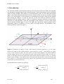
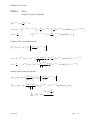
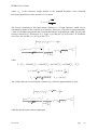
sample geometry is given in figure 1.
Figure 1: Definition of angles in spin echo neutron reflection geometry. k is the angle
r
between the path of the incident neutron (represented by vector k , indicated by the green
arrow, or the red arrow where the start of the vector has been shifted to the sample surface)
and the sample surface. #k is the angle the path of the incident neutron makes with the xyr
plane. p the angle between the path of the off-specular scattered neutron (vector p ) and the
sample surface and #p is the angle between the path of the off-specular scattered neutron and
the xy-plane. &s is the angle between the path of the off-specular scattered neutron and the
path of the not-scattered neutron.
In general the wave vectors are given by:
r 2
k=
24-4-2009
cos (
) cos ( k )
sin ( k )
cos ( k ) sin ( k )
k
r 2
p=
cos (
) cos ( )
sin ( )
cos ( ) sin ( )
p
p
p
p
p
page
3
SENRef User’s Guide
Throughout the program the small angle approximation for the determination of the wave
vectors is used, hence
r 2
k=
1
1
2
( k)
2
1
2
k
k
( k)
2
r 2
p=
1
1
2
( )
2
1
2
p
( )
2
p
p
p
The neutron beam of a reflectometer is always collimated in two directions. The first
direction, parallel to the sample surface is in general very wide, and the second direction
perpendicular to the surface is in general small, some mm to 1/10 of mm. The latter slit width
is important for the resulting profile resolution and determines also the coherence length of
the neutron beam along the sample surface. The former slit width is kept wide to keep the
beam intensity as high as possible as the reflected intensity will be orders of magnitude
smaller than the incident intensity (as much as 6 to 8 orders have been achieved).
The Spin Echo technique can be used to code a component of the direction of an individual
neutron in the beam and find out the component of the scattering angle in the same direction1.
If this direction is used along the wide slit direction, then also the scattering angle parallel to
the sample can be determined, yielding information on the sample surface in all directions.
The information obtained in the direction parallel to the surface are the sample surface
correlation functions and perpendicular to the surface the sample profile2.
1
J. Plomp, “Spin-echo development for a time-of-flight neutron reflectometer”, Thesis Delft University of
Technology, 2009
2
V.O. de Haan, “Coherence approach to neutron propagation in spin echo instruments”, 1st ed, BonPhysics
Research and Investigations B.V., 2007.
24-4-2009
page
4
SENRef User’s Guide
2. Start program
The program is written in Microsoft Visual Studio 2005 (Visual Basic) and will need the
.NET Framework. This will all ready be installed on your computer, installed at set-up, or you
should provide it yourself.
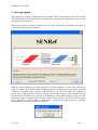
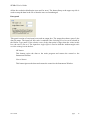
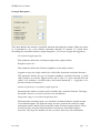
When the program is started a splash screen will pop up showing a disclaimer you have to
accept before the program continues:
Push the Accept button if you agree that the use of the program is at your own risk and no
rights or claims can be derived from using the program. If this button is pressed the program
continues, searching in the resources sub directory of the directory where the program is
stored, for a XML-formatted file that contains the default settings. If the program can not
locate the file in this directory, the user is prompted by a file input dialog box typical for the
operating system to indicate where the file can be found. The user can select a session data
file or press the CANCEL button. If this button is pressed the program issues a warning,
indicating that no session data file was loaded:
24-4-2009
page
5
SENRef User’s Guide
After pressing the OK button the program continuous with the default values of the program.
The above SENRef Warning dialog box will appear whenever the user does something
unexpected.
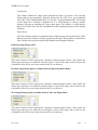
For all parameters tooltips are given, explaining shortly the use of the control that is pointed
at with the mouse.
The program has a button driven interface which consists of 1 tab control with 7 major tab
windows: Instrument, Sample, QxQyPlot, QxCuts and QyCuts, Fitting and Thanks and three
buttons Load Session, Save Session and Make Session Default.
Load Session button
This button enables the session data input. If pressed a file selection dialog will pop up
requesting a filename. The used extension is XML as the session data file is XML
formatted. If a valid filename is chosen the session data file will be loaded, enabling
the continuation of a previous session.
Save Session button
This button enables the session data output. If pressed a file selection dialog will pop
up requesting a filename. The used extension is XML as the session data file is XML
formatted. If a valid filename is chosen the session data file will be saved, enabling the
continuation in a future session.
Make Session Default button
This button enables the creation of a default session data file. If pressed the session
data is saved in the default session data file that will be automatically loaded at the
next start of the program.
Clicking the names of the tab windows will select that window. The Instrument Window is
used to define the instrument parameters and load the measured data. The Sample Window is
used to define the sample parameters, load sample profiles and perform calculations. The
QxQyPlot, QxCuts and QyCuts windows are used for diagnostic purposes and defining the
cuts. These windows work for either or both the loaded data, including the calculation of the
error bars (for QxCuts and QyCuts), and the calculated data. The Fitting window can be used
to fit the selected sample model to the data. The Thanks windows contains clickable images
yielding information about the program and theory behind the calculations used.
24-4-2009
page
6
SENRef User’s Guide
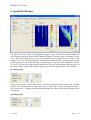
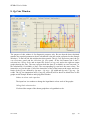
3. Instrument Window
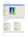
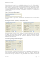
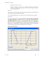
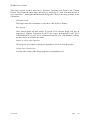
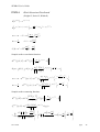
To the left the Instrument Window has 4 panels: Instrument, Reflected Angle Range,
Wavelength Range (or Incident Angle Range) and Data panel. To the right there is space for
viewing the data after loading. Depending on the status of the instrument panel and the data
loaded, graphs are given of the relevant neutron or X-ray intensity plots. At the bottom there
are two buttons: Load and Save.
Instrument panel
Time-Of-Flight mode:
Monochromatic mode:
The instrument panel consists of three selection boxes for the measurement type and a check
box for the Spin Echo mode, four input boxes Spin Echo Constant (or Footprint angle),
Incident Angle (or Wavelength), Resolution and Coherence length and a Load and Show
button.
24-4-2009
page
7
SENRef User’s Guide
Selection boxes measurement type
Select either Time-of-Flight (only for neutron scattering), Monochromatic Neutron or
Monochromatic X-Ray. In Time-of-Flight mode the second input box on the
instrument panel changes to the input box for the Incident Angle. In monochromatic
mode it changes to the one for the Wavelength. The first input box changes from Spin
Echo Constant in Time-Of-Flight mode into Footprint Angle in monochromatic mode.
In Time-of-Flight mode the 3rd panel from the top changes to the Wavelength Range
panel. In monochromatic mode it changes to the Incident Angle Range panel.
Check box Spin Echo
In Time-of-Flight mode, it is possible to indicate weather the measurements are made
with Spin Echo or without. Without Spin Echo only the non-polarized scattered
intensity can be calculated or loaded / saved. With Spin Echo the plus and minus
scattered intensity can be calculated or loaded / saved. As an extra in the Spin Echo
mode, the polarisation and the shim intensity can be shown. Further the input box Spin
Echo Constant and the Load button will be enabled.
Input box Spin Echo Constant
In Time-Of-Flight mode the spin echo constant is used. The input must be changed to
the desired value and depends on the setting of the apparatus. The value represents the
spin echo length in micrometers divided by the square of the wavelength of the
neutrons in nanometres.
Input box Footprint Angle
In Monochromatic mode the spin echo constant is not used, but the footprint angle is
important. The value represents the incident angle at which the incident beam just
covers the sample length in the direction of the beam. For larger incident angles the
beam footprint is reduced with the ratio sin(Footprint angle) / sin(Incident angle) and
the intensity with the square of this ratio. The input must be changed to the desired
value and depends on the setting of the apparatus.
Input boxes Incident Angle (or Wavelength), Resolution and Coherence length
These inputs must be changed to the desired values. The Incident Angle is the angle
between incident beam and sample surface. The resolution is the standard deviation of
the Gaussian distributed Incident Angle spread of the beam. The coherence length is
the width of a homogeneous, Gaussian distributed, mutual coherence function. As the
three variables are coupled (see chapter 6.1.1 of reference in footnote 2) changing one
will result in a corresponding change of the others. For SENRef the relation between
these parameters is:
rc =
1000
2
k
,
k
where rc is the Coherence Length in micrometer units,
the Wavelength in
nanometer, k the Incident Angle in milliradians and
k is the Resolution also
in milliradians.
24-4-2009
page
8
SENRef User’s Guide
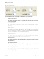
Load button
This button enables the empty beam polarization input. If pressed a file selection
dialog will pop up requesting a filename. Extensions are OUT (for a space delimited
file), OSV (for a TAB delimited file) or CSV (for a comma delimited file). The format
of the input file is defined in appendix B. If a valid filename is chosen, another
window will pop up enabling the correct data input. This window is called Import
Data File Window (See also the Load Button on the Grating Data panel on the Sample
Window).
Show button
The Show button enables investigation of the loaded empty beam polarization. If this
button is pressed a window will pop up showing the data. This window is called Show
Data Window (See also the Load Profile Button on the Sample Window).
Reflected Angle Range panel
This panel consists of three input boxes: Minimum, Maximum and Number. They define the
linear range and step over which the reflected angle is varied. This range will be used for the
calculations if the Scales from Data selection box is not checked.
Incident Angle Range panel (Available when in Monochromatic Mode)
This panel consists of three input boxes: Minimum, Maximum and Number. They define the
linear range and step over which the incident angle is varied. This range will be used for the
calculations if the Scales from Data selection box is not checked.
Wavelength Range panel (Available when in Time-Of-Flight Mode)
This panel consists of three input boxes: Minimum, Maximum and Number. They define the
linear range and step over which the wavelength is varied. This range will be used for the
calculations if the Scales from Data selection box is not checked.
24-4-2009
page
9
SENRef User’s Guide
Data panel
This panel consists of one input box, one output box and two selection boxes. The input box
is a number to change the logarithmic colour scale of the graphs. The output box is only
visible when a data file has been loaded and shows the name of the data file. The selection
boxes are the Scales from Data selection box and the 10 Log selection box:
Scales from Data selection box
If selected (checked) the calculation scales are the same as the data scales. If not
selected the calculation scales are as defined on the Instrument Window.
10 Log selection box
If selected (checked) the colour plot scale is logarithmic with base 10. If not selected
the scale is linear.
Save button
This button enables the data output. If pressed a file selection dialog will pop up requesting a
filename. Extensions are OUT (for a space delimited file), OSV (for a TAB delimited file) or
CSV (for a comma delimited file). If a valid filename is chosen the data will be saved under
that name. The format of the file is the same as of the input file (see Appendix A), but errors
will not be included.
Load button
This button enables the data input. If pressed a file selection dialog will pop up requesting a
filename. Extensions are OUT (for a space delimited file), OSV (for a TAB delimited file) or
CSV (for a comma delimited file). If a valid filename is chosen another window will pop up
enabling the correct data input. This window is called Import Measurement Window.
24-4-2009
page
10
SENRef User’s Guide
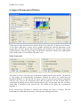
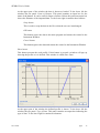
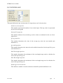
4. Import Measurement Window
To the upper left the window has two panels: Define Type and Name of Measurement Dataset.
To the upper right there is space for two graphs, showing the selected input data. At the
bottom there are three panels: Wavelength Range and Resolution (or Incident Angle Range
and Resolution), Scattered Angle Range and Resolution and Data. Finally at the right bottom
of the window there are two buttons OK and Cancel.
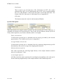
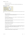
Define Type panel
or
This panel is used to select the type of data that is loaded with the selected file. The data file
is very simple, not containing this information. Initially the values are copied from the
Instrument Window. To the left side the panel consists of selection type buttons comparable
with the ones used in the Instrument panel and an input box for the incident angle or
wavelength depending on the selected measurement type. To the right side one can select
which data is included in the selected file. The format of the input file is defined in
appendix A.
If the selection box Polarized is checked, the selection box Swap is enabled. The box
interchanges the plus and min intensity, inverting the resulting polarization.
24-4-2009
page
11
SENRef User’s Guide
If the selection box Include Error is checked the selection box From File will be enabled. If
both selection boxes are checked the program expects the data to contain the errors, according
to the format of appendix A. If the selection box From File is not checked, but Including
Error is, the program assumes that the data in the file are raw neutron counts and the error is
calculated as the square root of the counts. If selection box Including Error is not checked, all
errors are set to 0.
Name of Measurement Dataset panel
This panel contains an input box for the name of the loaded dataset. It can be used for future
reference.
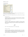
Wavelength or Incident Angle Range and Resolution panel
or
This panel contains 2 selection criteria: Input (nm or A) and Resolution type (File, Gaussian
and Block), three output and two input boxes. Minimum, Maximum and Number define the
range and number of data points in the data file. Relative and Absolute define the resolution
distribution (not used for now).
Scattered Angle Range and Resolution panel
This panel contains 2 selection criteria: Input (Degrees or milliradians) and Resolution type
(File, Gaussian and Block), three output and two input boxes. Minimum, Maximum and
Number define the range and number of data points in the data file. Relative and Absolute
24-4-2009
page
12
SENRef User’s Guide
define the resolution distribution (not used for now). The button Swap at the upper top side is
used to swap the data in the file so that the axes are interchanged.
Data panel
This panel consists of two input boxes and an output box. The output box shows (part of) the
data file name. The input box Min value is enabled if the Including Error box was selected in
the Define Type panel. If the relative error of the data point is larger than the value in this
box, the error is set to 0. The input box Angle Offset is used to shift the incident angle scale
over the value given in the box.
OK button
This button copies the data to the main program and returns the control to the
Instrument Window.
Cancel button
This button ignores the data and returns the control to the Instrument Window.
24-4-2009
page
13
SENRef User’s Guide
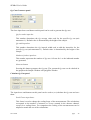
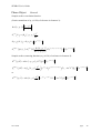
5. Sample Window
To the left side this window has four panels: Sample Surface Type, Specular Data, Grating
Data or Isotropic Data (or nothing) and Calculation Data. To the right side it has a selection
box Type, two output graphs, two buttons Calculate and Save, an input box Orders in colour
scale and a selection box 10 Log Scale. The panel Grating Data appears if a 1D or 2D profile
is selected. The panel Isotropic Data appears if an Isotropic profile is selected.
Sample Surface Type panel
This panel defines the type of profile or correlation function describing the sample. From this
function the scattering is calculated according to the approximation selected in the Calculation
Data panel. The panel has one selection box and two buttons and an output box.
24-4-2009
page
14
SENRef User’s Guide
Selection box
Several predefined sample surface types can be selected. An 1D or 2D surface type is
described by a height profile. An isotropic sample surface type is defined by a
Gaussian correlation function. The formula used depends on the selected
approximation and is given in Appendix C. The profile or correlation can be
predetermined or user defined.
Capillary Waves selection
The Gaussian roughness correlation function is given by:
C (r ) =
2
rmin
r
ln
+1
2
rmin
1
where
is the roughness and the correlation length. See also the reference
in footnote 3. The value for rmin is a cut-off value rmin = a / N , where
N = value of input box Number of points per correlation length
a = value of input box Integration range in correlation length
Gravitational Waves selection
The Gaussian roughness correlation function is given by:
C (r ) =
2
K 0 (r / +
)
where
is the roughness, the correlation length and K 0 the modified Bessel
function of zero-the order. See also the reference in footnote 3. The value for r
= 0 is cut-off for K 0 ( ) = 1 (
0.45689248915903589527).
Self-affine fractional selection
The Gaussian roughness correlation function is given by:
C (r ) =
2
e (r /
)2 h
where
is the roughness, the correlation length and h the so-called
jaggedness parameter. See also the reference in footnote 3.
24-4-2009
page
15
SENRef User’s Guide
Self-affine fract (anal) selection
Similar to Self-affine fractional, but calculated analytically following the
method described by R. Pynn, Phys. Rev. B, Vol.45, No 2, January 1992 p602612. See also appendix D.
Output box
The output box, just below the Load button, shows the filename of the loaded profile
(if present, other wise the output box is empty).
If a user defined height profile or correlation is selected, the button Load is enabled.
Load button
This button enables the profile input. Note that for a 1D or 2D user defined profile
the height distribution is loaded and for an isotropic defined profile the
correlation function. If pressed a file selection dialog will pop up requesting a
filename. Extensions are OUT (for a space delimited file), OSV (for a TAB delimited
file) or CSV (for a comma delimited file). The format of the input file is defined in
appendix B. If a valid filename is chosen another window will pop up enabling the
correct data input. This window is called Import Data File Window.
Import Data File Window
24-4-2009
page
16
SENRef User’s Guide
At the upper part of the window the data is shown as loaded. To the lower left the
window has one panel: Name of Dataset. This panel contains an input box for the
name of the dataset. It can be used for future reference. Below this panel an output box
shows the filename of the imported data. To the lower right it contains three buttons:
Swap button
This is used to swap the data in the file so that the axes are interchanged.
OK button
This button copies the data to the main program and returns the control to the
Instrument Window.
Cancel button
This button ignores the data and returns the control to the Instrument Window.
Show button
This button presents the used profile. If this button is pressed a window will pop up
showing the profile as it is defined. This window is called Show Data.
At the upper part of the window the defined profile is shown. To the lower left the
window has one panel: Type of Data. This panel contains an output box indicating the
type of data. To the lower right it contains two buttons:
24-4-2009
page
17
SENRef User’s Guide
Save button
This is used to save the data into a file. Extensions are OUT (for a space
delimited file), OSV (for a TAB delimited file) or CSV (for a comma delimited
file). If a valid filename is chosen the data will be saved under that name. The
format of the file is the same as of the input file (see Appendix B).
OK button
This button returns the control to the Instrument Window.
Specular Data panel
or
This panel defines the sample surface and the way the specular part of the reflectivity is
calculated. It consists of two selection boxes, Theory and Average Gamma, and one (or two in
X-Ray mode) input box (es) Gamma substrate (and at wavelength)
Theory selection box
If selected the specular part is calculated from the theory provided by the selected
approximation. The formula used is given in Appendix C.
Average Gamma selection box
If selected the specular part is calculated from the scattering length density profile
determined by the surface average of the height profile function.
Gamma substrate input box
This value represents the scattering length density of the sample substrate material
times 4 in nanometer-2 units.
at wavelength input box
In X-Ray mode this value represents the wavelength corresponding to the value given
for the scattering length density of the sample material in the Gamma input box.
24-4-2009
page
18
SENRef User’s Guide
Grating Data panel
This panel defines the height profile function describing the sample. Either by means of a
predefined or a user defined height profile function.
The panel has three check boxes, SA Rough, Gaussian Dist. and Gauss Envel, and 9 input
boxes.
SA Rough Check box
If checked the scattering is convoluted with the scattering determined by a Self-Affine
roughness as defined by the Isotropic Data panel. The values taken for the Self-Affine
roughness distribution are taken from that data.
Gauss Envelop check box
If checked the sample correlation function is multiplied by a Gaussian envelop
function with a correlation length given by the input box Correlation length. This
mimics a not perfect periodicity or represents an artificial resolution contribution. The
formula used is
e
1
2
r
rc
2
,
where r is the correlation distance and rc the correlation length.
Gauss Dist. check box
If checked the sample is described by a height profile function. The correlation
function is calculated assuming the grating is not perfect periodic, but has a Gaussian
correlated distribution. The formula used depends on the selected approximation and
is given in Appendix C. The height profile function can be predetermined or user
defined. This is determined by the Grating data panel.
24-4-2009
page
19
SENRef User’s Guide
Correlation length input box
This value determines correlation length of the sample correlation function in
nanometers. It is only enabled when the Gauss Envelop selection box is selected.
Gamma Layer input box
This value represents the scattering length density of the sample layer material times
4 in nanometer-2 units.
Height Input box
This value determines the sample height in nanometers. If a height profile function is
loaded it represents the total height of the loaded profile.
Period Input box
This value determines the sample repetition period in nanometers. If a height profile
function is loaded it represents the repetition period of the loaded profile.
DutyCycle Base Input box
This value determines the sample base width of either block or trapezium in % of the
period value.
Slope Input box
This value determines the slope in % of the trapezium. 100 % is an angle of 45
degrees. The minimum angle depends on the height of the sample, the period and the
dutycycle of the base.
In Plane Angle Input box
This value determines the orientation angle of the sample profile with respect to the
beam. For 0o the grating profile is parallel to the beam direction and for 90o it is
perpendicular.
Divergence In Plane Angle input box
This value determines the spread in the In Plane Angle parameter. The distribution
function is a block with a constant width and amplitude given by this value.
Number of points per In Plane Angle input box
This number determines the number of interval steps used to calculate the influence of
the divergence of the In Plane Angle parameter.
24-4-2009
page
20
SENRef User’s Guide
Isotropic Data panel
This panel defines the isotropic correlation functions describing the sample. Either by means
of a predefined or by a user defined correlation function. It consists of 5 input boxes
describing the correlation function, sample Roughness, Correlation Length and Jaggedness.
Correlation Length input box
This parameter defines the correlation length of the sample surface.
Roughness Input box
This parameter defines the Gaussian roughness of the sample surface.
Jaggedness input box (Only enabled for a Self-affine fractional correlation function)
This parameter defines the type of Gaussian roughness correlation function. A small
value produces an extreme jagged surface and a value of 1 gives smooth hills and
valleys. It is related to a fractal surface with fractal dimension 3 – Jaggedness. See
also the reference in footnote 3.
Number of points per correlation length input box
Determines the number of points used to calculate the correlation function. The larger
the number, the more accurate and slower the calculations.
Integration range in correlation length input box
Determines the maximum range over which the correlation function extends in units
of correlation lengths. The larger the range, the more accurate the results for small
momentem tranfer, and the less accurate the results for large moment transfer. These
can also be more accurate when the number of points per correlation length is
increased. The larger the number, the more accurate and slower the calculations.
24-4-2009
page
21
SENRef User’s Guide
Calculation Data panel
This panel defines the theory used to perform the scattering calculations and some parameters
needed to perform the calculations. The panel contains 2 input boxes and 3 selection boxes:
Number per Coherence length input box (for 1D profile)
This number determines the number of orders used to calculate the scattering for a
periodic structure. (It corresponds to the range of n in the summations of Appendix C).
In general, if the separate Qx-cuts can be distinguished in the scattering, then this
parameter can be 1. If they start to overlap, this number must be increased. If they
coincide (due to scattering in the z-direction only), to get an accurate result the number
must be taken large enough. A rule of thumb for an X-profile:
Number of points Coherence length =
= 1 + Period / Coherence length / Cos (In Plane Angle),
the Cos function changes into a Sin function for an Z-profile. It is wavelength
dependent, as the coherence length is wavelength dependent. The calculations are
slower if the number is larger.
Number per Coherence length input box (for 2D profile)
This number determines the number of intervals used to calculate the Fourier
transform of the 2D correlation function determined from the user defined height
profile function. The Fourier transform extends to 5 times the coherence length.
Number of points per Angle Div input box
This number determines the number of intervals used to calculate the influence of the
width of the interval of the scattered angle channels.
Selection box
This selection enables the selection of the theory used for the calculations. Options are
First Born approximation, Phase Object approximation, Distorted Wave Born
approximation (see Appendix C for detail) or Extended Phase Object approximation
(see Thanks Window, click on picture below text). The Extended Phase Object
approximation is not implemented for the Gaussian distribution of the profile’s. For
this approximation one can either choose the height to be constant, or the scattering
length density of the layer to be constant by selecting the appropriate radio button after
the Height input box or Gamma Layer input box. For this approximation it is also
possible to have a different scattering length density for the substrate and the layer.
Note that the colour of the DWBA selection box turns red if the calculations render an
unrealistic result, due to the imaginary part of the wave vector transfer becoming too
24-4-2009
page
22
SENRef User’s Guide
large negative. Then the criteria for the DWBA are not fulfilled. Roughly the criteria
are: small disturbances (less then a few nanometer in height) only close to the critical
edge, or far away from the critical edge.
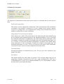
Type selection box
With this box the type of data shown in selected. Chose Shim, Plus intensity, Min intensity or
Polarization.
Calculate button
This button starts the calculations. It can take a while before it finishes. The bar directly to the
right indicates progress made. During calculations the Save button changes into a Stop button
that can be used for obvious reasons. After stopping in this way, the data the calculated is not
reliable!
Save button
This button enables the data output. If pressed a file selection dialog will pop up requesting a
filename. Extensions are OUT (for a space delimited file), OSV (for a TAB delimited file) or
CSV (for a comma delimited file). If a valid filename is chosen the data will be saved under
that name.
Orders in colour scale input box
The input box is a number to change the logarithmic colour scale of the graphs.
10 Log Scale selection box
If selected the output of the shown graph has a logarithmic scale.
24-4-2009
page
23
SENRef User’s Guide
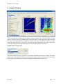
6. QxQyPlot Window
The purpose of this window is for diagnostic purposes only. The data calculated matches the
last calculation action performed on the Sample Window. The QxQy plot is calculated in such
a way that the integral over Qx, Qy of the scattering function gives the same value as the
integral over , Lp. To the left side this window has two panels: The Qx Range panel and the
Qy Range panel. To the right side it has a selection box 10 Log Scale and an input box Orders
in colour scale and two output graphs showing the plots for the calculations and the data. At
the bottom of the window three buttons appear: the Calculate button and two Save buttons.
Qx Range panel
This panel consists of three input boxes: Minimum, Maximum and Number and a button
Default. They define the linear range and step over which Qx is varied. Note that the unit of
Qx is micrometer-1. Pushing the default button changes the values to the range available in the
calculations.
Qy Range panel
24-4-2009
page
24
SENRef User’s Guide
This panel consists of three input boxes: Minimum, Maximum and Number and a button
Default. They define the linear range and step over which Qy is varied. Note that the unit of
Qy is nanometer-1. Pushing the default button changes the values to the range available in the
calculations.
Calculate button
This button starts the calculations. It can take a while before it finishes.
Save buttons
These button enable the data output. If pressed a file selection dialog will pop up
requesting a filename. Extensions are OUT (for a space delimited file), OSV (for a
TAB delimited file) or CSV (for a comma delimited file). If a valid filename is chosen
the data will be saved under that name.
Orders in colour scale input box
The input box is a number to change the logarithmic colour scale of the graphs.
10 Log Scale selection box
If selected the output of the shown graph have a logarithmic scale.
24-4-2009
page
25
SENRef User’s Guide
7. QxCuts Window
The purpose of this window is for diagnostic purposes only. Be sure that the data calculated
matches the required parameters (hence calculation is the last action performed on the Sample
Window). To the left side this window has three panels: The Qx Cuts Definition panel, the Qx
cuts Generator panel and the Calculate Qx Cuts panel. To the left bottom side it has a
selection box 10 Log Scale and an input box Orders in log scale and to the right an output
graph showing the cuts. The cuts represent both the data (if available) as error bars and / or
the calculations (if available) as lines. The corresponding Qx cuts have the same colour. The
intensities are just the sum of all of the intensities in the points between the upper and lower
limits of the Qx cut defined by Qx max = Qx avg + Qx width and Qx min = Qx avg - Qx
width. If Qx is equal to 0, the cut is the specular one between Incident Angle + Delta Angle
and Incident Angle – Delta Angle. The Qx cut summation areas (if any are selected) will be
shown as black lines on the graphs on the Sample Window and QxQyPlot Window.
Orders in colour scale input box
The input box is a number to change the logarithmic colour scale of the graphs.
10 Log Scale selection box
If selected the output of the shown graph have a logarithmic scale.
24-4-2009
page
26
SENRef User’s Guide
Qx Cuts Definition panel
or
This panel defines the Qx cuts by means of 6 input boxes and 1 selection box:
Number of cuts input box
This number represents the number of cuts in the figure. Each Qx value is represented
by one line in the graph.
Selected Cut input box
This number indicates from which Qx cut the values are indicated in the two lower
input boxes.
Qx avg input box
This number gives the average Qx value of the cuts. When equal to 0 the lowest Input
box of the current panel is changed to Delta Angle (unit milliradians), when different
from 0 the lowest Input box is Qx width (unit micrometer-1).
Delta Angle input box
This number determines the angle difference of the scattered angle between which the
intensities are added to find the specular cut (unit milliradians).
Qx width input box
This number determines the intervals used to add the intensities for the specific Qx cut
(unit micrometer-1).
Min Wavelength input box
This number determines the minimum of the wavelength range used to calculate the
cuts for the specific Qx cut.
Max Wavelength input box
This number determines the maximum of the wavelength range used to calculate the
cuts for the specific Qx cut.
24-4-2009
page
27
SENRef User’s Guide
Enable Qx Cut selection box
This indicates weather or not the selected cut should be plotted and fitted or not.
Qx Cuts Generator panel
The selection box, four input boxes and button on this panel can be used to generate the Qx
cuts.
Qx first order input box
This number determines the Qx average value of the first order cut used to add the
intensities for the specific Qx cut (unit micrometer-1).
Qx width input box
This number determines the Qx interval width used to add the intensities for the
specific Qx cut (unit micrometer-1).
Number of Positive orders Input box
This number represents the number of Qx cuts with a positive order. All cuts for 1 to
the indicated number are generated.
Number of Negative orders Input box
This number represents the number of Qx cuts with a negative order. All cuts for 1 to
the indicated number are generated.
Include specular selection box
If the selection box is checked the generated Qx cuts will include the specular one. For
the width of the specular one the resolution of the incident angle is taken (see
Instrument Window, Instrument Panel, Resolution input box).
Generate button
Pressing this button generates the Qx cuts. The generated Qx cuts can be checked in
the graph on the Sample Window and QxQyPlot window.
24-4-2009
page
28
SENRef User’s Guide
Calculate Qx Cuts panel
The input boxes and buttons on this panel can be used to (re-)calculate the Qx cuts and save
them.
Scale Factor input boxes
This factor is used to change the scaling factor of the measurements. The calculations
correspond to the number of neutrons or X-rays counted in the detector channel,
except for a scaling factor. For comparison the scaling of the measurements can be
adapted to match the one of the calculations.
Polarization Correction selection buttons
These buttons are visible if the polarization of the empty beam has been loaded using
the Load button on the Instrument panel on the Instrument Window. If Calc is selected
the calculated polarization is multiplied by the loaded empty beam polarization. If the
wavelength is outside the available wavelength range, the calculated polarization is set
to 0. If Data is selected the measured polarization is divided by the loaded empty
beam polarization. If the wavelength is outside the available wavelength range, the
measured polarization is set to 0. If None is selected no correction is done. Remember
to use the Calculate button to let the changed selection take effect.
Calculate button
Pressing this button (re-)calculates the Qx cuts. The Qx cuts can be checked in the
graph to the right.
Save button
This button enables the data output. If pressed a file selection dialog will pop up
requesting a filename. Extensions are OUT (for a space delimited file), OSV (for a
TAB delimited file) or CSV (for a comma delimited file). If a valid filename is chosen
the data will be saved under that name.
24-4-2009
page
29
SENRef User’s Guide
8. QyCuts Window
The purpose of this window is for diagnostic purposes only. Be sure that the data calculated
matches the required parameters (hence calculation is the last action performed on the Sample
Window). To the left side this window has three panels: The Qy Cuts Definition panel, the Qy
cuts Generator panel and the Calculate Qy Cuts panel. At the left bottom side it has a
selection box 10 Log Scale and an input box Orders in log scale and to the right an output
graph showing the cuts. The cuts represent both the data (if available) as error bars and / or
the calculations (if available) as lines. The corresponding Qy cuts have the same colour. The
intensities are just the sum of all of the intensities of the points between the upper and lower
limits of the Qy cut, defined by Qy max = Qy avg + Qy width and Qy min = Qy avg - Qy
width. The Qy cut summation areas (if any are selected) will be shown as black lines on the
graphs on the Sample Window and QxQyPlot Window.
Orders in colour scale input box
The input box is a number to change the logarithmic colour scale of the graphs.
10 Log Scale selection box
If selected the output of the shown graph have a logarithmic scale.
24-4-2009
page
30
SENRef User’s Guide
Qy Cuts Definition panel
This panel defines the Qy cuts by means of 6 input boxes and 1 selection box:
Number of cuts input box
This number represents the number of cuts in the figure. Each Qy value is represented
by one line in the graph.
Selected Cut input box
This number indicates from which Qy cut the values are indicated in the two lower
input boxes.
Qy avg input box
This number determines the value of the average Qy value the cuts should (unit
nanometer-1).
Qy width input box
This number determines the intervals used to add the intensities for the specific Qy cut
(unit nanometer-1).
Min Wavelength input box
This number determines the minimum of the wavelength range used to calculate the
cuts for the specific Qy cut.
Max Wavelength input box
This number determines the maximum of the wavelength range used to calculate the
cuts for the specific Qy cut.
Enable Qy Cut selection box
This indicates weather or not the selected cut should be plotted and fitted or not.
24-4-2009
page
31
SENRef User’s Guide
Qy Cuts Generator panel
The three input boxes and button on this panel can be used to generate the Qy cuts.
Qy first order input box
This number determines the Qy average value used for the specific Qy cut (unit
nanometer-1). Default value is determined by the height of the sample.
Qy width input box
This number determines the Qy interval width used to add the intensities for the
specific Qy cut (unit nanometer-1). Default value is determined by the height of the
sample.
Number of orders input box
This number represents the number of Qy cuts. All cuts for 1 to the indicated number
are generated.
Generate button
Pressing this button generates the Qy cuts. The generated Qy cuts can be checked in
the graph on the Sample Window and QxQyPlot window.
Calculate Qy Cuts panel
The input boxes and buttons on this panel can be used to (re-)calculate the Qy cuts and save
them:
Scale Factor input boxes
This factor is used to change the scaling factor of the measurements. The calculations
correspond to the number of neutrons or X-rays counted in the detector channel,
except for a scaling factor. For comparison the scaling of the measurements can be
adapted to match the one of the calculations.
24-4-2009
page
32
SENRef User’s Guide
Polarization Correction selection buttons
These buttons are visible if the polarization of the empty beam has been loaded using
the Load button on the Instrument panel on the Instrument Window. If Calc is selected
the calculated polarization is multiplied by the loaded empty beam polarization. If the
wavelength is outside the available wavelength range, the calculated polarization is set
to 0. If Data is selected the measured polarization is divided by the loaded empty
beam polarization. If the wavelength is outside the available wavelength range, the
measured polarization is set to 0. If None is selected no correction is done. Remember
to use the Calculate button to let the changed selection take effect.
Calculate button
Pressing this button (re-)calculates the Qy cuts. The Qy cuts can be checked in the
graph to the right.
Save button
This button enables the data output. If pressed a file selection dialog will pop up
requesting a filename. Extensions are OUT (for a space delimited file), OSV (for a
TAB delimited file) or CSV (for a comma delimited file). If a valid filename is chosen
the data will be saved under that name.
24-4-2009
page
33
SENRef User’s Guide
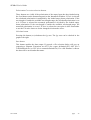
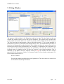
9. Fitting Window
The purpose of this window is for fitting the model to the data. The data fitted are the cuts
defined and enabled on the QxCuts and QyCuts Windows. The program only calculated the
point needed to determine these cuts. Lesser cuts and the smaller ranges increase the fit speed.
The fit is based on the minimization of the so called chi-squared, i.e. The average quadrate of
the difference between fit and data point divided by the error. The minimization procedure is
based on the Marquardt-Levenberg method. This method calculates the steepest decent from
the matrix inversion of the Jacobian matrix. If a change in a fit parameter has no influence (or
very small) on the calculated chi-squared, the possibility exist that the inversion of the
Jacobian matrix is singular and the fit does not converge to the (local) minimum. This is
indicated by the Matrix inversion indicator turning to red. The window has three control
panels, Select Fit Parameters, Define Fit Parameters and Fit Control and a results panel, Fit
Results and a button, Reset Fit.
Reset Fit button
Pressing this button initialized the model parameters. The start values are taken from
the Instrument and Sample Windows.
24-4-2009
page
34
SENRef User’s Guide
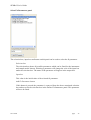
Select Fit Parameters panel
The selection box, input box and button on this panel can be used to select the fit parameter.
Selection box
The selection box shows all possible parameters which can be fitted for the instrument
and sample model chosen. Selecting a parameter will change the vale of the input box
under the selection box. The name of the parameter will appear in the output box.
Input box
This value is the initial value of the selected fit parameter.
Add Fit Parameter button
If this button is pressed the parameter is removed from the above mentioned selection
box and moved to the selection box in the Define Fit Parameters panel. This parameter
will now be fitted.
24-4-2009
page
35
SENRef User’s Guide
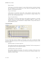
Define Fit Parameters panel
The selection box, three input boxes and three buttons on this panel can be used to set the
right upper and lower limits of the fit parameters. The smaller the range the faster and reliable
the algorithm will find the desired minimum.
Selection box
The selection box shows all parameters are fitted. Selecting a parameter will change
the vale of the input boxes under the selection box.
Min Value input box
This value determines the lower limit of the fit parameter selected in the selection box.
Start Value input box
This value determines the initial value of the fit parameter selected in the selection
box.
Max Value input box
This value determines the upper limit of the fit parameter selected in the selection box.
24-4-2009
page
36
SENRef User’s Guide
Remove button
If this button is pressed the parameter is removed from the above mentioned selection
box and returned to the selection box in the Select Fit Parameters panel. This
parameter will is not fitted anymore.
Copy to model button
If this button is pressed the actual value of the parameter selected in the above
selection box is copied to the parameter in the Instrument or Sample Window. The
previous value of this parameters is lost.
Copy All to model button
If this button is pressed the actual value of all possible fit parameters in the both
selection boxes of the Select and Define Fit Parameter Panels are copied to the
respective parameters in the Instrument or Sample Window. The previous values of
these parameters are lost.
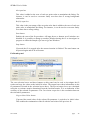
Control Fit panel
The four input boxes and two buttons on this panel can be used to control the fitting
procedure. The graph at the lower side of the panel shows the chi-squared as function of the
iteration number.
Maximum number of iterations input box
This number determines the maximum number of iterations. The fit can stop sooner, if
the required accuracy in chi-squared is reached.
10 LOG Iteration accuracy input box
This number determines fit accuracy. It is used as a measure of the step size to
determine the gradient of the function and it determines the minimum change in chisquared to continue fitting.
24-4-2009
page
37
SENRef User’s Guide
Abs input box
This value is added to the error of each cut point value to manipulate the fitting. For
instance, it can be used to overcome faulty error bars due to wrong background
subtraction.
Rel(%) input box
This value is the percentage of the cut point value that is added to the error of each cut
point value to manipulate the fitting. For instance, it can be used to overcome faulty
error bars due to wrong scaling.
Start button
Enables the start of the fit procedure. All input boxes or buttons on all windows are
disabled. It is possible to change to another Window during the fit to investigate its
progress on either the Sample, QxCuts or QyCuts Windows.
Stop button
If pressed the fit is stopped after the current iteration is finished. The start button can
be pressed again and de fit will restart.
Fit Results panel
The two selection boxes and three buttons on this panel can be used to investigate the fit
results and copy the values to the initial fit values. The output boxes show information on the
fit parameters selected in the selection boxes above. The Spread output boxes are calculated
using the co-variance matrix determined from the Jacobian matrix. It is an indication of the
accuracy of the selected fit parameter. The Correlation output box is the correlation between
the selected fit parameters.
Copy to Start Value button
If pressed the actual value of the selected fit parameter is copied to its initial value.
This enables the continuation of the fit with the end value of the previous fit.
24-4-2009
page
38
SENRef User’s Guide
Copy All to Start Value button
If pressed the actual value of all fit parameters are copied to their initial value. This
enables the continuation of the previous fit.
24-4-2009
page
39
SENRef User’s Guide
10. Thanks Window
The purpose of this window is for information purposes only. You can find this guide by
clicking on the upper left picture. The theoretical background for the calculations can be
found in the book ‘Coherence approach to neutron propagation in spin echo instruments’.
This is opened if the lower left picture is clicked. Clicking on the Extended Phase Object
gives information about these calculations. Clicking the right pictures opens the home pages
of the corresponding institutes.
24-4-2009
page
40
SENRef User’s Guide
Appendix A: Format of Data file
The files are simple ASCII files. The input format is as follows:
Up Spin or Down Spin or Non-Polarized
Without Errors:
[Y0 Y1
Y2 ….. Yn Yn+1//
X1 D11 D12 ….. D1n//
X2 D21 D22 ….. D2n//
…
Xm Dm1 Dm2 ….. Dmn//
Xm+1]
Up Spin or Down Spin or Non-Polarized
With Errors:
[Y0 Y1 Y1 Y2 Y2 ….. Yn Yn Yn+1 Yn+1//
X1 D11 E11 D12 E12 ….. D1n E1n//
X2 D21 E21 D22 E22 ….. D2n E2n//
…..
Xm Dm1 Em1 Dm2 Em2 ….. Dmn Emn//
Xm+1]
Polarized
Without Errors:
[Y0 Y1 Y1 Y2 Y2 ….. Yn Yn Yn+1 Yn+1//
X1 P11 M11 P12 M12 ….. P1n M1n//
X1 P21 M21 P22 M22 ….. P2n M2n//
…..
Xm Pm1 Mm1 Pm2 Mm2 ….. P1m M1m//
Xm+1]
24-4-2009
page
41
SENRef User’s Guide
Polarized
With Errors:
[Y0 Y1 Y1
Y1
Y1
Y2 Y2
Y2
Y2
….. Yn Yn
Yn
Yn Yn+1 Yn+1//
X1 P11 EP11 M11 EM11 P12 EP12 M12 EM12 ….. P1n EP1n M1n EM1n//
X2 P21 EP21 M21 EM21 P22 EP22 M22 EM22 ….. P2n EP2n M2n EM2n//
…..
Xm Pm1 EPm1 Mm1 EMm1 Pm2 EPm2 Mm2 EMm2 ….. Pmn EPmn Mmn EMmn//
Xm+1]
Where:
‘ [‘ indicates start of file
‘ //‘ indicates end of line
‘]’ indicates end of file
‘…..’ indicates user required repetition of sequence
Y0 is a number: Not used
Yi (i=1..n) : start values of scattered angle interval i (In ascending order)
Yi+1 (i=1..n) : end values of scattered angle interval i (In ascending order)
Xj (j=1..m): start value of incident angle (Monochromatic mode) or wavelength (TOFmode) interval j (In ascending order)
Xj+1 (j=1..m): end value of incident angle (Monochromatic mode) or wavelength
(TOF-mode) interval j (In ascending order)
Dij: Data values for Xj;Yi
Eij: Error in data values for Xj;Yi (standard deviation)
Pij: Data values Up Spin for Xj;Yi
EPij: Error in data values Up Spin for Xj;Yi (standard deviation)
Mij: Data values Down Spin for Xj;Yi
EMij: Error in data values Down Spin for Xj;Yi (standard deviation)
24-4-2009
page
42
SENRef User’s Guide
Appendix B: Format of Data file
(1 Dimensional Profile and Empty beam polarization)
The files are simple ASCII files. The input format is as follows:
[Y0 Y1//
X1 D1//
X2 D2//
…
Xm Dm]
Where:
‘ [‘ indicates start of file
‘ //‘ indicates end of line
‘]’ indicates end of file
‘…..’ indicates user required repetition of sequence
Y0 is a number: Not used
Y1 is a number: Not used
Xj (j=1..m): Distance (Profile mode) or wavelength (Polarization mode) in [nm]
Dj: Data values for Xj: Height in [nm] (Profile mode) or Polarization
24-4-2009
page
43
SENRef User’s Guide
Appendix C: Background of performed calculations.
In general the calculations are done using the equations described in chapter 6 of the reference
of footnote 2. To speed up the calculations it was assumed that the incident mutual coherence
function on the sample position was homogeneous and Gaussian distributed with a large
coherence length in the beam direction and a small one in the direction perpendicular to it.
The coherence length is the standard deviation of the Gaussian distribution.
In principle the spin-echo signal for a grating must be determined using eqs. (7.14) and (7.15)
of reference in footnote 2. However, if there is only structure in the z-direction and the in
plane angle is 0, then eq. (7.24) can be used to speed up the calculations. If some in-plane
angle different from 0 is used in principle this is wrong, for the scattering in the x-direction.
Then the Number per Coherence length parameter must be increased to find the correct spinecho signal for the scattering.
In the following the basic equations for the several sample types and approximations are
given.
24-4-2009
page
44
SENRef User’s Guide
DWBA
General
Sample surface correlation function
(Combination of eqs. (6.96) to (6.99) of reference in footnote 2):
(0,0)
s
G
Spec
s
G
T ( py )
p 2y
r
p
=
A
R
p
( ) s ( y ) 2 = As
4
(
)
OffSpec
s
G
8 py
p
r r r
r
p, k , r// = Gs(0,0) ( p ) 1 + y E e
p 'y
(
(
2
2
)
r
2 ip ' y H ( rs )
1
*
r r
4 p y2 T ( k y )
r r r
i ( y ) H ( r// + rs )
(0,0) r
p, k , r// = Gs ( p )
E
e
2
T ( py )
y
)
i
yH
(
r
( rs )
E e
i
yH
r
( rs )
)
2
Sample surface scattering function
(Combination of eqs. (6.104) to (6.107) of reference in footnote 2):
r r
S k p, k = e
(
)
r r
iQ// r//
r r r
Gs p, k , r// d 2 r//
(
)
r r
r r
r r
Sk p, k = SkSpec p, k + S kOffSpec p, k
(
S
Spec
k
)
(
(
r r
p, k = 4
)
2
r r
SkOffSpec p, k = As
(
)
)
As
2
(
T ( py )
2
2
8 py
T ( py ) T ( k y )
16
2
2
)
(
r
py
Q// 1 +
E e
p 'y
( )
e
r r
iQ// r//
E e
i
( y)
*
)
r
2 ip ' y H ( rs )
r r
H ( r// + rs ) i
yH
2
1
r
( rs )
d 2 r//
4
2
2
( ) (
r
Q// E e
i
yH
r
( rs )
)
y
or
r r
SkOffSpec p, k = As
(
24-4-2009
)
2
T ( py ) T ( k y )
16
2
2
e
r r
iQ// r//
e
i
yH
r
( r// )
d 2 r//
2
4
2
2
(Q ) E (e
r
//
i
yH
r
( rs )
)
2
y
page
45
2
SENRef User’s Guide
DWBA
Gaussian Random Distribution
(standard deviation , average µ, complex constant q):
(
E e
r
iqH ( rs )
E e
i
)=e
2 2
q / 2+iµ q
*
( y ) H ( rr// + rrs )
r
1
C r// = A
s
As
i
yH
r
( rs )
2
=e
y
(
(
2
r
C ( r// )
* 2
)e
y
)
r
r r
H ( rs ) H rs + r// d 2rs , C(0) =
( y)
2
/2
2
Sample surface correlation function:
Spec
s
G
(
(
p
r r r
r
p, k , r// = Gs(0,0) ( p ) 1 + y e
p 'y
)
2 p '2y
2
2
r r r
r 4 p T (ky )
GsOffSpec p, k , r// = Gs(0,0) ( p ) y2
e
T
p
(
)
y
y
(
)
)
2
1
{ }
Re
2
y
2
2
e
y
r
C ( r// )
1
Sample surface scattering function:
S kSpec
(
r r
p, k = 4
)
r r
S kOffSpec p, k = As
(
24-4-2009
)
2
T ( py )
As
2
2
2
8 py
T ( py )T ( ky )
16
2
2
e
Re
(
r
py
Q// 1 +
e
p 'y
( )
( )
2
y
2
e
r r
iQ// r//
2 p '2y
2
e
y
r
C ( r// )
2
)
2
1
1 d 2 r//
y
page
46
SENRef User’s Guide
DWBA
Block
(Height H, Period L, Width D)
(
E e
iqH ( xs )
) = 1 + DL ( e
0
x<D
D
x<
E e
i
1)
iqH
*
( y ) H ( x + xs )
L
2
i
yH
( xs )
E e
i
(
D
1 e
L
=1
*
( y ) H ( x + xs )
i
yH
) + Lx ( 2e { } cos ( H Re{ }) 1
2D
{ }
= 1+
e
cos ( H Re { } ) 1)
(
L
{ y}
2 H Im
( xs )
H Im
y
H Im
{ y}
2 H Im
e
y
y
y
Sample surface correlation function:
r r r
r
D py
p, k , r// = Gs(0,0) ( p ) 1 +
e
L p 'y
G
(
0
x<D
D
x<
Spec
s
(
)
)
2 ip ' y H
2
1
2
r r r
r 4 py T ( k y ) x
GsOffSpec p, k , r// = Gs(0,0) ( p )
2
T ( py ) L
y
(
)
2
r r r
r 4 py T ( k y ) D
GsOffSpec p, k , r// = Gs(0,0) ( p )
2
T ( py ) L
y
(
L
2
2
D
D
+
L
L
2
)
( 2e
( 2e
{ y}
H Im
{ y}
H Im
(
cos H Re {
(
cos H Re {
y
})
y
})
1 e
1 e
{ y}
2 H Im
{ y}
2 H Im
)
Sample surface scattering function:
S kSpec
(
r r
p, k = 4
)
2
r r
S kOffSpec p, k = As
(
)
As
2
T ( py )
2
2
8 py
T ( py )T ( k y )
4
2
n=
24-4-2009
( )
( Qz )
y
×
,n 0
(
r
D py
Q// 1 +
e
L p 'y
( Qx
(e
2n
2 H Im
)
{ y}
)
2 ip ' y H
2e
1
{ y}
H Im
(
cos H Re {
y
}) + 1) ×
D
L
sin 2 n
(n )
2
2
page
47
)
)
SENRef User’s Guide
DWBA
Block Gaussian Distributed
(Height H, Period L, Width D)
(
E e
r
iqH ( rs )
E e
i
)=e
2 2
q / 2+iµ q
*
( y ) H ( rr// + rrs )
0
x<D
D
L
x<
2
C ( 0) =
i
yH
r
C r// =
r
( rs )
H
=e
(
D x
L
2
r
C r// =
H
D
L
D
L
2
2
r
C ( r// )
* 2
)e
( y)
y
2
/2
2
2
D
D
1
L
L
= H2
2
2
y
Sample surface correlation function:
Spec
s
G
(
p
r r r
r
p, k , r// = Gs(0,0) ( p ) 1 + y e
p 'y
(
)
OffSpec
s
G
(
2 p '2y
2
4 p y2 T ( k y )
r r r
(0,0) r
p, k , r// = Gs ( p )
e
2
T
p
(
)
y
y
)
0
x<D
D
L
x<
2
GsOffSpec
)
2
1
{ }
Re
2
y
2
r r r
r 4 py T ( k y )
p, k , r// = Gs(0,0) ( p )
e
2
T ( py )
y
(
)
OffSpec
s
G
(
2
2
e
{ }
2
y
Re
2
r r r
r 4 p T (ky )
p, k , r// = Gs(0,0) ( p ) y2
e
T ( py )
y
)
y
2
{ }
Re
2
y
r
C ( r// )
1
y
e
2
D x
L
2
H2
2
y
e
H2
D
L
D
L
2
1
2
1
Sample surface scattering function:
S
Spec
k
(
r r
p, k = 4
)
2
r r
S kOffSpec p, k = As
(
)
2
H2
×
n=
,n 0
(H
24-4-2009
y
As
2
y
T ( py )T ( ky )
Qx
2
2
8 py
4
2
e
2 Im
(
r
py
Q// 1 +
e
p 'y
( )
( )
y
2
2
2 p '2y
2
)
2
1
( Qz ) ×
y
2n
L
) + ( 2n
2 2
2
T ( py )
)
2
"
"1
"
"
$
H2
2
y
sin 2n
2n
D
L
+ cos 2n
D
L
e
D 2
H
L
2
y
!
#
#
#
#
%
page
48
SENRef User’s Guide
Phase-Object
General
Sample surface correlation function
(Fourier transform of eq. (6.124) of reference in footnote 2):
RPO ( k y , p y ) =
(0,0)
s
G
py
p 'y
ky
p 'y
2
r
p y2
k = As RPO ( p y , p y ) 2
4
( )
( ) (
r
r r r
GsSpec p, k , r// = Gs(0,0) k E e
(
)
r
r r r
GsOffSpec p, k , r// = Gs(0,0) k
(
)
r
iq y H ( rs )
)
2
RPO ( k y , p y )
( )R (
py , py )
PO
(
r r
iq H ( r + r )
E e y ( // s
r
H ( rs ) )
) E (e
r
iq y H ( rs )
)
2
Sample surface scattering function (eq. (6.124) of reference in footnote 2):
r r
SkSpec p, k = As RPO ( p y , p y ) p 2y
(
)
2
( ) (
r
Q// E e
p2
r r
SkOffSpec p, k = As RPO ( k y , p y ) y2
4
or
(
S
OffSpec
k
(
)
p 2y
r r
p, k = As RPO ( k y , p y ) 2
4
24-4-2009
)
e
e
r r
iQ// r//
r r
iQ// r//
e
r
iq y H ( rs )
)
2
(
r r
iq H ( r + r )
E e y ( // s
r
iq y H ( r// )
d 2 r//
2
r
H ( rs ) )
4
2
)d r
2
//
2
4
(Q ) E (e
r
//
2
2
(Q ) E ( e
r
r
iq y H ( rs )
//
r
iq y H ( rs )
)
)
2
2
page
49
SENRef User’s Guide
Phase-Object
Gaussian Random Distribution
(standard deviation , average µ, complex constant q):
(
E e
r
iqH ( rs )
)=e
(
r r
iq H ( r + r )
E e y ( // s
r
1
C r// = A
s
2 2
q / 2+iµ q
r
H ( rs ) )
As
)
=e
q 2y
(
2
(
r
C ( r// )
)
)
r
r r
H ( rs ) H rs + r// d 2rs , C(0) =
2
Sample surface correlation function:
r
r r r
GsSpec p, k , r// = Gs(0,0) k e
(
)
( )
r
r r r
GsOffSpec p, k , r// = Gs(0,0) k
(
)
2 2
qy
RPO ( k y , p y )
( )R (
PO
py , py )
e
2 2
qy
(
e
r
q 2y C ( r// )
)
1
Sample surface scattering function:
r r
S kSpec p, k =
(
)
2
r
(Q ) A R (
//
s
PO
p y , p y ) p 2y e
r r
S kOffSpec p, k = As RPO ( k y , p y ) p y2e
(
24-4-2009
)
2 2
qy
e
r r
iQ// r//
2 2
qy
(
e
r
q 2y C ( r// )
)
1 d 2 r//
page
50
SENRef User’s Guide
Phase-Object
Block
(Height H, Period L, Width D)
(
E e
iqH ( xs )
) = 1 + DL ( e
0
x<D
D
x<
(
E (e
1)
iqH
iq H ( x + xs )
E e y(
L
2
) = 1 + 2Lx ( cos ( q H ) 1)
)
) = 1 + 2LD ( cos ( q H ) 1)
H ( xs ) )
iq y ( H ( x + xs ) H ( xs )
y
y
Sample surface correlation function:
r
D
D
r r r
GsSpec p, k , r// = Gs(0,0) k 1 2
1
1 cos ( q y H )
L
L
(
0
D
)
x<D
x<
(
( )
OffSpec
s
G
(
r
r r r
p, k , r// = Gs(0,0) k
)
RPO ( k y , p y )
( )R (
py , py )
PO
(
)
(
)
( )R (
py , py )
PO
x
L
2 cos ( q y H ) 1
RPO ( k y , p y )
r
r r r
GsOffSpec p, k , r// = Gs(0,0) k
L
2
)
(
D
D
+
L
L
)
2 cos ( q y H ) 1
D
L
2
2
Sample surface scattering function:
r r
SkSpec p, k =
(
)
2
r
(Q ) A R ( p ,
//
s
PO
y
r r
SkOffSpec p, k = As RPO ( k y , p y ) p y2
(
)
×
n=
24-4-2009
,n 0
p y ) p y2 1 2
( Qz ) 2 (1
( Qx
2n
)
(
D
D
1
1 cos ( q y H )
L
L
)
)
cos ( q y H ) ×
D
L
sin 2 n
(n )
2
page
51
SENRef User’s Guide
Phase-Object
Block Gaussian Distributed
(Height H, Period L, Width D)
(
E e
r
iqH ( rs )
)=e
(
r r
iq H ( r + r )
E e y ( // s
0
x<D
D
L
x<
2
C ( 0) =
2 2
q / 2+iµ q
)=e
r
H ( rs ) )
r
C r// =
H
(
r
C ( r// )
2
D x
L
2
r
C r// =
2
q 2y
H
D
L
2
2
D
L
2
)
D
D
1
L
L
= H2
Sample surface correlation function:
r
r r r
GsSpec p, k , r// = Gs(0,0) k e
(
0
D
)
x<D
( )
OffSpec
s
G
L
x<
2
(
2 2
qy
RPO ( k y , p y )
r
r r r
p, k , r// = Gs(0,0) k
)
OffSpec
s
G
(
( )R (
py , py )
PO
r
r r r
p, k , r// = Gs(0,0) k
)
e
RPO ( k y , p y )
( )R (
PO
py , py )
2 2
qy
e
e
2 2
qy
q 2y H 2
e
D x
L
q 2y H 2
D
L
D
L
2
1
2
1
Sample surface scattering function:
r r
S kSpec p, k =
(
)
2
r
(Q ) A R (
//
s
PO
r r
S kOffSpec p, k = As RPO ( k y , p y ) p y2
(
)
H 2 q y2
×
n=
,n 0
Qx
2n
L
( H q ) + ( 2n )
24-4-2009
2
2 2
y
2
"
"1
"
"
$
p y , p y ) p 2y e
2 2
qy
( Qz ) ×
sin 2n
H 2 q y2
2n
D
L
+ cos 2n
D
L
e
D 2 2
H qy
L
!
#
#
#
#
%
page
52
SENRef User’s Guide
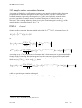
Born Approximation
Similar to Phase-Object Approximation except that RPO ( k y , p y ) is replaced by
RFB ( k y , p y ) =
24-4-2009
2
4 p y2 ( p y
ky )
2
.
page
53
SENRef User’s Guide
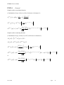
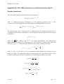
2-D sample surface correlation function
According to Sinha3, for a reflectometer geometry (no angular resolution in the direction
perpendicular to the beam and parallel to the sample surface, here the z-direction) the
scattered intensity is given by the integral over Qz (this was implicitly assumed in the
previous, but there the sample surface correlation function was either in the z or x
direction.).The resulting intensity is then given by the Fourier integral over the Qx of the
sample surface correlation function for z = 0.
DWBA
General
r r
Sample surface scattering function (which only holds if S kOffSpec ( p, k ) is integrated over Qz):
r r
S k p, k = e
(
)
r r
iQ// r//
r r r
Gs p, k , r// d 2 r//
(
)
so
S
Spec
k
(
r r
p, k = 4
)
2
r r
S kOffSpec p, k = As
(
)
T ( py )
As
2
2
2
8 py
T ( py ) T ( k y )
8
2
(
r
py
Q// 1 +
E e
p 'y
( )
( Qz )
iQx x
e
E e
i
)
r
2 ip ' y H ( rs )
*
( y ) H ( xerx + rrs )
2
1
i
yH
r
( rs )
dx 2
( Qx ) E ( e i
yH
r
( rs )
)
2
y
According to eq. (7.14) of reference in footnote 2 the 2-shim count rate is proportional to this
Sample surface scattering function integrated over the source area, detector area and sample
area. The 2-flip count rate can be found in a similar way using eq. (7.16), where PE in the
ideal case (eq. (7.8) PR = 0) is cos(Qy lse ) , hence:
r r
SkOffSpec
p, k = As
, flip
(
)
2
T ( py )T ( k y )
8
2
( Qz )
e
iQx x
E e
i
r
( y ) H ( xerx +lse + rrs )
*
i
yH
r
( rs )
dx 2
( Qx ) E ( e i
yH
y
while the specular part remains unchanged.
Similar expression can be derived for the Phase-Object and Born Approximations.
3
Sinha et al., Phys. Rev. B 38 (4) 1988, p2297-2312
24-4-2009
page
54
r
( rs )
)
2
SENRef User’s Guide
Appendix D: Self-Affine Gaussian correlation function and its
Fourier transform.
The Self-Affine Gaussian correlation function is defined as:
r
CSA ( r// ) =
2
( r// / )2 h
e
,
where = standard deviation of distribution, h is the jaggedness parameter and
correlation or cut-off length. The expectation value of such a distribution is given by:
(
E e
)=e
r r
r
iQ( H SA ( r// + rs ) H SA ( rs ) )
Q2
(
2
r
CSA ( r// )
)
is the
,
The specular part of the scattering can be calculated from the standard deviation alone,
according to the formulas in Appendix C. The off-specular part is proportional to the Fourier
transform of :
e
where Q =
y
r
Q 2CSA ( r// )
for DWBA and Q = q y
1,
for Born approximation and Phase-object
approximation. According to R. Pynn (Phys. Rev. B, Vol.45, No 2, January 1992 p602-612)
As long as q y2 2 < 1, a reasonable approximation of this value is found by inserting
e
where
Q 2CSA ( x )
1=
2
e
c0 ( , h ) c1 ( , h )
x
c2 ( , h )
x
2
,
= Q , c1 ( , h ) and c2 ( , h ) are parameters which depend only weakly on
but
strong on h, and c0 ( , h ) depends weakly on h and stronger on . Pynn does not give values
for these coefficients but it can be found that a reasonable approximation is given by:
2
c0 ( , h ) =
c1 ( , h,
c2 ( , h,
)=
)=
1
2
1
4
2
"
$
+
4
16
+
,
1 h2 !
#,
( h) %
1 h2 !
1
,
#+
( h ) % 2 coh 2
"1
$
2
!
,1 h 2 # ,
$e
%
( h ) = max "
24-4-2009
page
55
SENRef User’s Guide
where coh is the coherence length defined as the standard deviation of the Gaussian
Resolution distribution of the neutron or X-ray beam:
e
I ( x ) = I0
2
x
1
2
coh
.
2
coh
The Fourier transform of this approximate function is a Voight function, which can be
calculated by means of the complex error function. However, it can also be approximated by
a sum of a weighted Lorentzian and Gaussian distribution, with different width. The way this
is done is shown by P. Thomson et al. (J. Appl. Cryst. 20 (1987) p79-83) and G. K. Wertheim
et al. (Rev. Sci. Ins. 45 (11) (1974) p1369-1371).
(
cos ( qx x ) I ( x ) e
0
=
2 c0 ( , h )
I0
e
e
c1 ( , h )
x
c2 ( , h )
x
2
coh
2
)
Q 2CSA ( x )
"
"
"
qx
"1 + 4
$
1 dx =
+ (1
2
)
ln ( 2 )e
4ln ( 2 )
qx
2
!
#,
#
#
#
%
where
=(
5
G
+ 2.69269
L
4
G
+ 2.42843
2
L
3
G
+ 4.47163
3
L
2
G
+ 0.07842
2
= 1.36603
G
L
- 0.47719
= 2 ln ( 2 ) c2 ( , h,
G +
5
L
)
1
5
,
3
+ 0.11116
L
4
L
),
= c1 ( , h,
L
L
,
).
The 2-flip count rate can be found in a similar way, where the approximation is used:
cos ( qx x ) I ( x ) e
Q 2 CSA
(
2
x 2 + lse
)
1 dx =
0
I0
2
2 c0 ( , h ) c1 ( , h )lse c2 ( , h )lse
e
coh
2
"
"
"
qx
"1 + 4
$
2
+ (1
)
ln ( 2 )e
4ln ( 2 )
qx
2
!
#
#
#
#
%
while the specular part remains unchanged.
24-4-2009
page
56