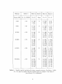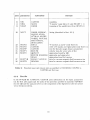
1
January 1996
~-lnstltuut
voor Plasmalyslca Rljnhulzen
Assoclatle Euratom-FOM
Postbus 1207
3430 BE Nieuwegein
Nederland
Edisonbaan 14
3439 MN Nieuwegein
Tel. + 31(0)3D-6096999
Fax. +31(0)30-6031204
CASTOR
Installation and User Guide
S. POEDTS, H.A. HOLTIES, J.P. GOEDBLOED,
G.T.A. HUYSMANS*, and W. KERNER*
*JET Joint Undertaking, Culham, United Kingdom.
RIJNHUIZEN
REPORT
96-229
Contents
1 Introduction
1.1 Resistive MHD eigenvalue problem
1.2 Projections and discretization
1.3 Eigenvalue solvers . . . . . . .
1
1
2 Installation guide
2.1 CASTOR and satellite programs . . . . . . . . .
2.2 Installation of REVISE . . . . . . . . . . . . . .
2.3 Installation of PPPLIB, HGOLIB, and EISLIN
2 .4 Installation of CASTOR . . . . . . . . . . . . .
7
7
3
User guide
3.1 Setting the dimensions . . . . . . . .
3.2 Pre-compiling, compiling, and linking
3.3 Input files . . . . . . . . . .
3.3.1 Namelist NEWRUN
3.3.2 Namelist NEWLAN
3.3.3 Mapping file .
3.3.4 T-matrix .
3.4 Submitting a job
3.5 Output files . . .
3.5.1 Listing ..
3.5.2 Vector plot files
3.5.3 Plot file . . . .
2
4
7
7
8
9
9
10
10
11
13
13
13
13
15
15
15
16
A REVISE
A. l Introduction . . . . . . .
A.2 Contents and use . . . .
A.3 Installation of REVISE .
A.4 IBM-Vlvl version of REVISE .
A.5 List of files . . . . . . . . . . .
17
17
17
18
18
19
B Installation script for PPPLIB
20
C Installation script for HGOLIB
21
References
22
1
Introduction
The aim of this 'Installation and user guide' for the program CASTOR is to provide
practical information for the installation of the program and for using it to determine
the ideal or resistive MHD spectrum, or part of it (e.g. instabilities or 'gap modes')
of axisymmetric toroidal plasmas. For a more technical and detailed description of the
applied numerical methods the reader is referred to the literature cited below.
CASTOR is a Fortran 77 program that solves the linear, resistive MHD eigenvalue
problem in a general toroidal geometry, where the equilibria are assumed to be axisymmetric. The eigenfunctions are essentially two dimensional since their dependence on the
toroidal angle can be described with one toroidal mode number (due to the axisymmetry
of the equilibrium).
CASTOR is used by many people and different versions of the program are available.
The REVISE package (see Appendix A) is used too keep track of the different versions of
the program. This installation and user guide applies to version 9e.
1.1
Resistive MHD eigenvalue problem
CASTOR considers the resistive MHD equations 1 linearized around a static axisymmetric equilibrium. The required information about the equilibrium is passed to CASTOR
through the 'equilibrium mapping file' produced by the equilibrium code HELENA [6].
=#
In CASTOR, a coordinate system (s, (), r/;) is used. The coordinate s
= )1/J/1/J1
labels the magnetic flux surfaces (7/J is the poloidal flux [6]). The coordinate rjJ is the usual
toroidal angle of the cylindrical (R, Z, r/;) coordinate system and the poloidal angle () is
determined such that the field lines are straight in the (0, r/;) plane, i.e.:
dr/;
d(J =
q(?jJ).
(1)
More information on the coordinate system, e.g. the metric coefficients, can be found in
the PhD thesis of Guido Huysmans [1].
The equilibrium density p0 can be chosen arbitrarily since it does not appear in the
Grad-Shafranov equation. In CASTOR, the following equilibrium density profiles can be
chosen:
Po
Po(s) = [1 - (1 - D)s 2 )]",
Po
Po(s) = (1 - D1s 2 )(1 + Ds 2 ),
Po(s) = 1 + Ds 2 + D 1 s4 + D2s 6 + D3s 8 ,
Po
(2)
(3)
(4)
where D, D 1 , D 2 , D 3, and v are input parameters. However, other density profiles can
easily be implemented in the code.
The linear resistive MHD equations are made dimensionless by normalizing the lengths
to the major radius of the equilibrium (RM, the radius of the magnetic axis), the magnetic
field to the equilibrium toroidal field at the position of the magnetic axis (B 0 ), and the
density to the equilibrium density at the magnetic axis (p 0 ). [Notice that the distance and
the magnetic field are normalized differently in HELENA and CASTOR. The distances
1
There also exists a version of CASTOR that includes thermal conduction and radiation \vhich is used
to study the thermal MHD spectrum [11]
1
and the magnetic field are re-scaled in HELENA when the mapping file for CASTOR is
produced.] The normalization of the other quantities follow from these, e.g. the velocity
B 0 / ,;µr;po. Hence,
is normalized with the Alfven velocity at the magnetic axis, i.e. VAo
the following normalizations are used:
=
-t
RM
I,
µoP
B;f
-t
P,
µoRM J
Bo
-t
J,
~µopo
B(f
-t
T,
p
Po
v
VAo
7]
µoRMVAo
-t
p,
-t
v,
-t
'ij'
B
Bo
VAo
RM
tE
VAoBo
-t
B,
-t
t,
-t
E,
where k 8 denotes the Boltzmann constant and m the mean particle mass. Below, only
dimensionless quantities are considered and the notation is simplified by dropping the
bars.
Using the vector potential A:
(5)
B = \7 x A,
instead of B itself, the resistive MHD eigenvalue problem can written in the following
form (in dimensionless units):
),p,
),poV1
),poT1
>,A,
-\7 · (pov1),
-\7(poT1 + p1T 0 ) + (\7 x B 0 ) x (\7 x Ai) - B 0 x (\7 x \7 x Ai),
-pov1 · 'VTo - (1- l)po\7 · V1+271(1- l)(\7 x Bo)· (\7 x \7 x A,),
-B 0 xv 1 -ry\7x\7xA 1 ,
(6)
(7)
(8)
(9)
with the time dependence of the linear perturbations taken to be ~ e' 1• The eigenvalue
), can be complex. The Ohmic term in Eq. (8) has been neglected in CASTOR.
1.2
Projections and discretization
The above system of linear MHD equations can be written in the matrix form:
LU=),RU,
(10)
where L and R are differential operators and U is the state vector defined by
(11)
In CASTOR, the Galerkin method is used and the test functions in the weak form
are chosen to be equal to the discretization functions of the state vector U. The actual
variables used in the numerical solution of the eigenvalue problem are defined as follows.
2
l
For the velocity, vi, the following representation is chosen, which is basically the ERATO
represention [10].
(12)
where J = \17/J/''ils. In terms of the contravariant components v'
and v¢ = Vi · \1 </; one gets simple combinations:
-
v2
= if
F
=vi·
\ls, v 0
B
¢)
(qv - v ,
=Vi·
\10,
(13)
where F = RB¢. For the vector potential, on the other hand, a covariant representation
is chosen:
A= -iAi \1 s - A2 \1B + A3 \1</J.
(14)
In terms of the covariant components A,, A 0 , and A¢ this yields
(15)
Finally, the perurbed density and temperature are multiplied with s:
(16)
so that the actual state vector used in the numerical solution reads:
(17)
The components of the state vector are discretized by means of a combination of cubic
Hermite and quadratic finite elements for the radial (s-) direction and a truncated series of
Fourier modes for the poloidal direction. Due to the considered axisymmetric equilibrium,
the dependence on the toroidal angle can be described by a single Fourier mode. This
yields
Af2
,1,. t)
- k ( s, (I ''-Pi
U
/\r
k
hk ( )
k
hk ( ) ) imO in¢ At
= '\""'
L '\""'
L (amjl
JI s + amj2 j2 s e
e
e '
(18)
m=AI1 j=l
where k labels the eight components of 0, m labels the Fourier harmonics in the poloidal
direction and j labels radial grid points. Not~ce that t_:vo finite elements, hJi (s) and hJ2 ( s),
are used in each radial gridpoint. For vi, A 2 , and A 3 cubic Hermite finite elements are
used, while p, v2 , v3 , T, and Ai are approximated by quadratic finite elements [8].
With two finite elements per variable and per grid point, the total number of unknowns
(a~ 1 , and a~n 12 ) amounts to 2 x 8 x M x N"' with Jvl = Jvl2 -Jvl1 +1 the number of poloidal
Fourier harmonics and N, the number of radial gridpoints. In the Galerkin procedure the
discretization (18) is used in the system (10) and the weak form of this system is obtained
by multiplying it with each of the 2 x 8 x M x Nr finite elements and integrating over the
plasma volume [8]. The application of the Galerkin procedure then yields an algebraic
system of the form
(19)
A·V=AB·V,
where A is a non-Hermitian matrix and B a positive-definite matrix. Both A and B are
tridiagonal block matrices with sub-blocks of dimension 16iV/ x 16Jvl (see [1] where the
matrix elements of A and B are given explicitely).
3
The resistive MHD system (10) is of order six in s and, hence, the solution is fully
determined when six boundary conditions are specified. When the plasma is surrounded
by a perfectly conducting wall at the plasma boundary (s = 1), the normal component
of the velocity and the magnetic field and the tangential electric field must vanish at the
wall. On the axis, regularity conditions need to be specified. In terms of the variables
used in CASTOR one gets:
il1(s=l)=O,
(20)
v1(s=O)=O,
(21)
at the wall and
at the magnetic axis. For the case where the plasma is surrounded by a vacuum and an
ideally conducting wall, the boundary conditions are discussed in [l], Chapter 4.
1.3
Eigenvalue solvers
Above we have seen that the Galerkin formulation of the resistive MHD eigenvalue problem leads to the complex non-Hermitian matrix eigenvalue problem 19. CASTOR contains
five different solvers for the numerical solution of this eigenvalue problem. For more information of numerical methods in non-Hermitian eigenvalue problems see the review paper
by Kerner [7].
Solver 1 uses the standard QR algorithm of the LINPACK library to determine the
complete spectrum of eigenvalues. However, the QR algorithm transforms the banded
matrices in full matrices and the resulting memory requirements restrict the spatial resolution considerably. As a matter of fact, only small problems with a relatively low number
of harmonics and radial grid points can be solved with the QR algorithm (see Table (1)).
Solvers 2, 3, and 4 apply so-called 'inverse vector iteration' schemes to calculate single
eigenvalues. These solvers are used when one is only interested in a few modes, e.g.
the largest positive eigenvalues in MHD stability studies or 'gap modes' (discrete global
modes in continuum gaps). As the inverse vector iteration algorithm conserves the band
structure of the matrices, the memory requirements are much less restrictive and much
larger problems (much higher spatial resolutions) can be treated (see Table (1)). The
three inverse vector iteration solvers differ in the way the matrices are stored and, hence,
they have different memory requirements. Solver 2 uses a standard band storage mode
and keeps both matrices in core. This is the fastest inverse vector iteration solver in
CASTOR but the most demanding as far as computer memory is concerned. Solver 3 is
an 'out of core' solver which means that the matrices are are stored on disk. This has
the advantage that very big problems can be handled with matrices that do not fit into
the central memory of the computer. The disadvantage is of course that a lot of I/O is
required to read/write parts of the matrices from/on disk which makes this solver slow.
Solver 4 keeps the matrices in core but stores them in a more efficient way than solver 2
does. As a result, the memory requirements are less restrictive than for solver 2 but with
this solver more CPU time is needed for the same job. A disadvantage of the inverse
vector iteration solver is that a fairly accurate initial guess has to be supplied in order
to find an eigenvalue. In principle, the solver iterates towards the eigenvalue closest to
the initial guess. In practice, the initial guess must typically be within a factor of two or
three of the actual eigenvalue to get convergence.
4
Solver 5, finally, is a Lanczos solver. This is a kind of combination of the two kinds
of solvers described above. It computes more than one eigenvalue at once, typically 50
eigenvalues, but it does not generate full matrices so that fairly big problems with high
spatial resolutions can be handled. A major disadvantage is that the Lanczos algorithm
is not as 'reliable' as the QR algorithm for non-Hermitian problems. The results depend
sensitively on the provided initial guesses in the studied window of the complex eigenvalue
plane.
5
Memory
Solver 1
Solver 2
Solver 3
Solver 4
Solver 5
Mwords (MB)
M x Nr (NDIMJ)
M x Nr
Mmax
M x Nr
MxN,.
4 (32)
< 59
3 x 128
5 x 45
7 x 23
11
3 x 250
5 x 89
7 x 44
3 x 84
5 x 30
7 x 15
8 (64)
< 86
3 x 271
5 x 97
7 x 49
9 x 29
17
3 x 530
5 x 191
7 x 97
9 x 58
3 x 177
5 x 64
7 x 32
9 x 19
16 (128)
< 123
5 x 201
7 x 10²
9 x 61
11 x 41
13 x 29
25
5 x 396
7 x 202
9 x 121
11 x 80
13 x 57
5 x 132
7 x 67
9 x 40
11 x 27
13 x 19
32 (256)
< 175
5 x 408
7 x 208
9 x 125
11 x 84
13 x 60
15 x 44
37
5 x 805
7 x 410
9 x 249
II x 166
13 x 118
15 x 88
5 x 269
7 x 137
9 x 83
11 x 55
13 x 39
15 x 29
64 (512)
< 249
7 x 420
9 x 254
11x170
13 x 121
15 x 91
17 x 70
19 x 56
21 x 46
53
7 x 831
9 x 503
11 x 336
13 x 240
15 x 180
17 x 140
19 x 111
21 x 91
7 x 277
9 x 168
11 x 112
13 x 80
15 x 60
17 x 47
19 x 37
21 x 30
128 (1024)
< 352
9x510
11 x 341
13 x 244
15 x 183
17 x 142
19 x 114
21 x 93
75
9 x 10¹²
11 x 678
13 x 485
15 x 364
17 x 283
19 x 226
21 x 185
9 x 338
11 x 226
13 x 162
15 x 121
17 x 94
19 x 75
21 x 62
Table 1: Possible spatial resolutions for given computer memory. For Solver 1 (QR)
111 x Nr must be smaller than the number given in column 2. For Solver 3
(out-of-core) Nr is 'unlimited'.
6
1
2
Installation guide
This installation guide contains information to install CASTOR from scratch, i.e. assuming none of the help programs (see below) has been installed yet. First, it is explained
what subroutine libraries are used by CASTOR. Next, it is explained how to install these
subroutine libraries and the program CASTOR.
2.1
CASTOR and satellite programs
CASTOR is not a stand-alone program. It makes use of PPPLIB (Plasma Physics Plot
LIBrary) subroutines for generating graphics and of HGOLIB (Hans GOedbloed LIBrary)
subroutines for the numerics. However, both PPPLIB and HGOLIB are written in standard Fortran 77, so these subroutine libraries are portable. They need to be installed
first, before running CASTOR. In addition, CASTOR uses some BLAS routines (Basic
Linear Algebra Subroutines) and subroutines from EISPACK and LINPACK, all available
on Cray (standard). On other machines, the required EISPACK and LINPACK routines
need to be linked to CASTOR after compilation. They are provided in the file eislin.f
which needs to be installed as a library first. Moreover, on Crays CASTOR uses some
standard Cray routines. On other machines, these routines are replaced by HGOLIB
routines and NAG routines.
Moreover, CASTOR and PPPLIB are provided in REVISE format. This means REVISE needs to be installed first. More information on the use of REVISE and on how to
install this package is given in Appendix A.
Hence, the following files are required for a successful installation of CASTOR version 9e, in addition to REVISE: cas9e.source, ppp15e.source, hgolib.f, eislin.f,
ppplib.mk, hgolib.mk, eislin.mk. The latter three files are Unix scripts which create
the libraries PPPLIB, HGOLIB, and EISLIN as discussed below.
2.2
Installation of REVISE
First of all, the REVISE package needs to be installed. The way this is done is described
in Appendix A.
2.3
Installation of PPPLIB, HGOLIB, and EISLIN
CASTOR 9e works with version 15e of PPPLIB. To install this version of the Plasma
Physics Plot library the file ppp15e. source first needs to be pre-compiled. The resulting
fortran file has to be split in different files, one for each subroutine. This can be done with
the 'fsplit' command. Next, each of these files needs to be compiled and the compiled
files have to be put in a library (with the 'ar' command). For Unix machines, a script
is available to do all this with just one command. The script is called ppplib. mk. Its
contents is printed out in Appendix B.
The installation of HGOLIB is very similar to the installation of PPPLIB except for
the fact that HGOLIB is not provided in REVISE format so that the pre-compilation step
is not required here. Again, a script is available to install HGOLIB on Unix machines.
This script is called hgolib.mk. Its contents is printed out in Appendix C.
7
The installation of EISLIN is only required on computers other than Cray and is
identical to the installation of HGOLIB. Hence, it suffices to replace 'hgolib' by 'eislin'
each time it occurs in the script hgolib .mk (see Appendix C) to install EISLIN on Unix
machines.
2.4
Installation of CASTOR
CASTOR is programmed in a modular structure and consists of the following parts:
PRESET: initialization of input parameters
TEST: built-in test cases
EQUIL: module specifying the equilibrium
VACUUM: module computing vacuum perturbation
MATl-5: module computing the matrices A and B
SOLVl-5: module containing the different eigenvalue solvers
DIAG 1-5: module containing the diagnostic routines
However, as mentioned above, CASTOR is provided in REVISE format. Hence, the source
file cas9e. source contains the main program as well as all the modules. This makes the
installation of CASTOR very simple. It suffices to make a directory, e.g. castor/, and to
copy the file cas9e. source to it.
8
3
User guide
This user guide describes the different steps required to run CASTOR successfully. All
input parameters are described as well as all the output produced by a successful run of
the code.
3.1
Setting the dimensions
Before compiling CASTOR, one has to specify some parameters in the source file of the
code. These parameters determine the dimensions of the vectors and matrices required in
the different algorithms. The parameters are to be specified in the COMDECKs COMMAX and COMPAR at the beginning of the source file. In COMDECK COMMAX one
has to specify:
LANZ = number of Fourier harmonics used for equilibrium quantities (must be lower
than or equal to MANZ);
MANZ= number of Fourier harmonics used for perturbed quantities (usually MANZ =
LANZ);
MDIF =difference between two succeeding Fourier harmonics of the perturbed quantities
(usually MDIF = 1, but for cylindrical plasmas with elliptical cross-sections MDIF
= 2 since even and odd Fourier numbers decouple in that case);
LMAX = number of Fourier harmonics used for the Fourier transforms of equilibrium
quantities (LMAX > LANZ, usually LMAX = 30)
LVANZ = number of Fourier harmonics used for vacuum equilibrium quantities (similar
to LANZ);
lv!VANZ = number of Fourier harmonics used for vacuum perturbed quantities (similar
to MANZ, must be equal to LVANZ);
LVMAX = number of Fourier harmonics used for the Fourier transforms vacuum equilibrium quantities (similar to LMAX);
NG MAX = maximum number of radial grid points.
The other parameters in COMDECK COMMAX do not need to be changed. In order
to connect the vacuum correctly to the plasma, LVANZ must be equal to lv!VANZ and
LVMAX and at least twice the maximum m-value specified (see below).
In COMDECK COMPAR one has to specify:
KILWOR = number of 64-bit words that can be used by the code;
NDIMl = dimension of the matrices generated by the QR-algorithm.
Both these parameters depend on the resolution specified in COMDECK COMMAX (see
above). An estimate of the resolutions that fit in a given core memory (specified by
KILWOR) can be found in Table (1) (for each of the solvers). The recommended value
for NDIMl is 16 x NG x MANZ
9
3.2
Pre-compiling, compiling, and linking
First, cas9e. source needs to be pre-compiled. The resulting fortran file cas9e. f can
then be compiled and linked to PPPLIB and HGOLIB. On a Cray computer the following
two commands do the job:
1) pre cas9e
2) cf77 -o cas9e -lnag -Wf"-em -1 cas9e.lst" cas9e.f $HOME/libs/ppplib.a
$HOME/libs/hgolib.a
and putting them in one script makes it even easier.
3.3
Input files
CASTOR uses NAMELIST formatting to read in data from input unit 'NIN' which is
specified in COMDECK COMPIO (the default is NIN= 10). Two namelists are defined,
viz. NEWRUN and NEWLAN. The parameters in namelist NEWRUN determine the
solver that is used, the radial resolution, the mode numbers, the plasma density, and the
output diagnostics. The parameters in namelist NEWLAN determine input and output
parameters for the Lanczos solver only.
In order to test the solvers after installation, a test case has been built in in CASTOR.
This test case is based on a well-known Solovev equilibrium, so that the results can
be compared to other numerical codes, such as NOVA, ERATO, and PEST [9]. The
definitions of the inverse aspect ratio and the ellipticity (or elongation) used in CASTOR
differ from those used by Solovev:
E
b
a
(i - Jl -
4E~)
2Es
Es
R
,
(22)
(23)
where Es and Es denote the inverse aspect ratio and the ellipticity as defined by Solovev,
respectively. The inverse transformation formulae read:
(1
Es
+ E2 )'
= (~) 1f1.
(24)
(25)
For the test case that is built in in CASTOR we have Es = 1/3 and Es = 2.
The s-grid can be accumulated in two points s 1 and s 2 , e.g. in order to resolve two
(nearly-)singular layers or a singular layer and a boundary layer. This is done in the
subroutine MESHAC which arranges the grid points such that the integral of a given
function is the same for all intervals [s;, s;+iJ· The function is specified in FGAUS as:
fa+ (1 - fa)
(26)
°'
10
1
where f 8 is a constant ( < 1) 'back ground function' that can be used to influence the
number of grid points that participate in the accumulation, and s 1 , o- 1 and s2 , o-2 determine
the centers and widths of the Gaussian functions that are used for the mesh accumulation.
The parameter a is a weight factor that allows to obtain a different degree of accumulation
in the points s 1 and s2 (a < 1). The parameters s 1 , s2 , o- 1 , and o- 2 are determined in
namelist NEWRUN (see below), but the paramters f 8 and a are specified in the code,
viz. in subroutine EQUIL (!8 = BGF=0.3 and a= FACT=l.).
3.3.1
Namelist NEWRUN
MODE = control parameter, switch for used solver and testcases:
0: termination of execution;
1: QR algorithm;
2: Inverse vector iteration, in-core solver;
3: Inverse vector iteration, out-of-core solver;
4: Inverse vector iteration, in-core version of out-of-core solver;
5: Lanczos algorithm;
11-15: testcase, Solovev equilibrium with ts = 1/3 and Es = 2 (t = 0.381966,
b/a = 1.9631867, see Sect. 3.3), solver 1 - 5;
EQNAME = name of the equilibrium (printed out as info on listing);
NLTORE = logical switch parameter:
.T.: toroidal equilibrium;
.F.: cylindrical equilibrium;
NG = number of radial grid points (:".:NG MAX);
RFOUR(l) =the lowest poloidal mode number (others are computed with MANZ and
MDIF);
NTOR = the toroidal mode number;
ETA = the plasma resistivity (17);
ASPECT = the aspect ratio (for NLTORE = .F. only);
QOZYL =the value of the safety factor at the magnetic axis (q 0 );
SIGl =parameter for mesh accumulation (see Eqn. (26));
SIG2 =parameter for mesh accumulation (see Eqn. (26));
XRl =parameter for mesh accumulation, first acc. point (see Eqn. (26));
XR2 = parameter for mesh accumulation, second acc. point (see Eqn. (26) );
R\VALL = position of the wall;
NVPSI = number of radial points in the vacuum metric;
NGV = number of radial points in the vacuum potential solution;
SIGV = sigma for mesh accumulation in the vacuum at the plasma-vacuum interface;
IEQ = parameter to select the equilibrium density profile:
1: density profile given by Eq. (2);
2: density profile given by Eq. (3);
3: density profile given by Eq. (4);
11
IDPOW =parameter v for density profile (see formula (2));
DSURF =parameter D for density profile (see formulas (2), (3), and (4));
DSURFl =parameter D 1 for density profile (see formulas (3), and (4));
DSURF2 =parameter D 2 for density profile (see formula (4));
DSURF3 =parameter D 3 for density profile (see formula (4));
NDIAGFK = print switch for Fourier components of the metric;
YSHIFT(i) = i-th estimate of the eigenvalue for inverse vector iteration (i <:; 100); for
solver 3, the values of VSHIFT are calculated automatic:
NRS = number of automatic shifts of the real part
NIS = number of automatic shifts of the imaginary part
DRS = size of the automatic shifts of the real part
DIS = size of the automatic shifts of the imaginary part
(solver
(solver
(solver
(solver
3 only);
3 only);
3 only);
3 only);
EPS = relative accuracy of the eigenvalue (for vector iteration only);
NPLOT = plot switch for solver 1-4, number of plots for QR solver, solvers 2 - 4: no
diagnostics if NPLOT = O;
Xlv!INQR(i) = lower limit x-axis for i-th QR-plot;
Ylv!INQR(i) = lower limit y-axis for i-th QR-plot;
XMAXQR(i) = upper limit x-axis for i-th QR-plot;
YMAXQR(i) = upper limit y-axis for i-th QR-plot;
ALPHIN = multiplication factor for equilibrium temperature, !!! HANDLE \VITH
CARE !!! ALPHIN SHOULD BE EQUAL TO ONE !!!;
IAS = switch parameter for symmetry in equilibrium:
0: up-down symmetric equilibrium;
1: asymmetric equilibrium;
IBYAC =switch parameter for writing vacuum field data (only if .NE. O);
GAMMA = ratio of specific heats;
IVAC = switch parameter for shape of wall around vacuum:
1: wall shape identical to plasma shape but RWALL times larger with respect to
geometric axis (default);
2,3: the wall radius with respect to geometric axis is given as a Fourier series with
elements specified in FW(l,. . .,NF\V) (see below);
4: use JET wall given in procedure JETGEO (only for IAS.EQ.1!);
F\V = array with Fourier clements of vacuum wall (should have the same normalization
as RMIN);
NF\V = number of elements in FW (see above);
RMIN =minor radius plasma used to scale wall radius (IVAC = 2, 3, 4). For JET wall:
minor radius in meters;
ZCNTR = shift (in meters) of the plasma center with respect to the vacuum wall midplane (IVAC = 4);
12
1
3.3.2
Namelist NEWLAN
ISTART = switch parameter:
0: start with shift (EWSHIFT) and computation of the T-matrix;
1: read T-matrix from disk (see Sect. 3.3.4);
ISTOP
= switch
parameter:
< 0: write T-matrix on disk and continue computation;
~
0: write T-matrix on disk and stop;
KMAX = dimension of the T-matrix;
MXLOOP = maximum number of shifts;
!SHIFT = switch parameter controlling the shifts:
=
1: makes shifts for EWSHIFT and OWS(l:NUS), in this case specify:
NUS: number of given shifts in addition to EWSHIFT;
OWS: vector with the specified shifts;
else: makes shifts for EWSHIFT and region determined by:
XLIML: minimum real part of investigated region;
XLIMR: maximum real part of investigated region;
YLIMB: minimum imaginary part of investigated region;
YLIMT: maximum imaginary part of investigated region;
IHOLE: .TRUE.: there is a region XHOLEL, XHOLER, YHOLEB,
YHOLET, part of the region XLIML, XLIMR, YLIMB, YLIMT, within
which no eigenvalues are to be searched for;
XHOLEL: minimum real part of the hole;
XHOLER: maximum real part of the hole;
YHOLEB: minimum imaginary part of the hole;
YHOLET: maximum imaginary part of the hole;
3.3.3
Mapping file
CASTOR needs a mapping file of the equilibrium. This file is created by HELENA.
For a description of its contents, see the 'HELENA user and installation guide' [6].
CASTOR reads the equilibrium mapping file in on the input unit 'NMAP' specified in
COMDECK COMPIO. The default specification is NMAP = 12.
3.3.4
T-matrix
When Solver 5 (Lanczos) is used with !START = 1 (see Sect. 3.3.2) the 'T-matrix' has
to be supplied. CASTOR reads it in from unit 'NIN2' which is specified in COMDECK
COMPIO (default: NIN2 = 11). The T-matrix can be computed with the option !START = 0 (see Sect. 3.3.2).
3.4
Submitting a job
CASTOR is usually run in batch because it requires a lot of core memory and usually
the amount of core memory is limited for interactive jobs. When submitting CASTOR
in batch, memory and maximum run time have to specified. These parameters determine
13
the jobclass in which the job will run and depend on the specified resolution and solver.
The memory is determined by the parameter KILWOR (see Sect. 3.1). Also, the namelist
input file needs to be allocated to unit 10, i.e. the input file must be called fort.10, and
the equilibrium mapping file needs to be allocated to unit 12 (NMAP = 12 is the default,
see COMDECK COMPIO). The following example script makes a new directory, copies
the file sol203.data to fort.10 and the file sol203.mapping (for the built-in test case) to
fort.12, runs cas9e, and renames the output files on a Cray computer (see below).
#! /bin/sh
# This is a shell script to run CASTOR in batch
#Usage: qsub castor
# Job parameters
#
==============
#QSUB -lM 64.0mw
#QSUB -lT 60
#QSUB
# Working directory
#
=================
mkdir $HOME/castor/Test
cd
$HOME/castor/Test
# File definitions
#
================
cp $HOME/castor/sol203.data
cp $HOME/castor/sol203.mapping
# Run
# --assign -0 -b 20 -s
assign -0 -b 20 -s
assign -0 -b 20 -s
assign -0 -b 20 -s
$HOME/castor/cas9e
# Output
# ======
mv fort. 10
mv fort. 20
mv fort.25
mv fort.26
mv fort.27
mv CASPLOT
rm fort. 12
cos
cos
cos
cos
fort.10
fort.12
u: 15
u: 16
u: 17
u: 18
input.data
listing.data
flowplot. data
qrplot.data
vacuumfield.data
plot .data
14
# End of shell script
3.5
Output files
The CASTOR output is specified in the diagnostics module DIAG which contains three
parts, viz. DIAGl, which determines the output for Solver 1 (QR), DIAG234, which
determines the output for the inverse vector iteration solvers (2, 3, and 4), and DIAG5,
which determines the output for Solver 5 (Lanczos). The output is different for the
different solvers and some output is only generated for debugging pruposes. Below, only
the 'standard' output of CASTOR is described.
The CASTOR standard output consists of three files, viz. a 'listing' with information
on the input parameters, the equilibrium that was used in the run, and the convergence
procedure in case of the inverse vector iteration solvers; a 'flowplot file' with the information on the velocity field that is required to make a 'flowplot' with flowplot. f (this file
is an input file for flowplot .f); and a 'plot file' which is a postscript file which contains
plots of parts of the spectrum for solvers 1 and 5 and plots of the components of the
eigenvector for solvers 2, 3, and 4. More details on each of these output files is given
below in the following subsections.
3.5.1
Listing
The listing is printed out on unit 'NOUT' which is specified in COMDECK COMPIO.
The default unit number is 20. The listing contains:
1) a print-out of the input parameters;
2) a print-out of some calculated parameters, such as the dimension of the matrices, q1 ,
R 0 , etc.;
3) information on the equilibrium after the rescaling with respect to the given value of
qo (QOZYL);
4) information on the s-grid that is used (can be accumulated);
5) information on the iteration procedure (inverse vector iteration solvers) or the obtained
eigenvalues (solvers 1 and 5).
3.5.2
Vector plot files
The inverse vector iteration solvers provide information on the velocity field and the
magnetic field in a 'vector plot files'. The velocity flowplot file is printed out on unit 25.
Together with the 'vector plot file' from HELENA, which contains the information on
the grid points on which the velocity components are specified by CASTOR, the program
flowplot. f can make a flow plot of that eigenvector.
The program vacf ield. f makes a similar 'vector plot' of the vacuum magnetic field,
using the data printed out by CASTOR on units 27 and 28.
The output files described above are the main output files. There are more output
files used by CASTOR. An overview and short description is given below in Table 2.
15
unit
parameter
subroutine
contents
10
11
12
NIN
NIN2
NMAP
CASTOR
SOLV5
IODSK
namelists
'T-matrix' (only Solver 5 with !START= 1)
mapping of the equilibrium (from HELENA)
20
NOUT
listing (described in Sect. 3.5.1)
22
23
24
25
26
NOUT2
NOUT3
NOUTP
NOUTV
NO UTE
27
28
NOUTVB
NOUTB
IODSK, MESHAC,
EQUILV, FKEQ,
FFTRAN, SPLINE,
VFKEQ, VACUUM,
SOLV1-SOLV5,
DIAG(l,234,5)
SOLV5
CASTOR
CASTOR
EIGVFK
QRPLOT
EIGVFK (DIAG234)
DIAG5
EQVAC, VACUUM
DIAG234
Table 2:
3.5.3
'T-matrices a and /3' (only Solver 5)
order of T-matrix and eigenvalues (only Solver 5)
text for first plot pages (input parameters)
velocity data for vector plot of flow
eigenvalues found by QR
eigenvalue and eigenvector
eigenvalues fourd by Lanczos
data for vacuum magnetic field reconstruction
data for vacuum magnetic field reconstruction
Standard input and output units as specified in COMDECK COMPIO in
CASTOR and their use.
Plot file
In the PPPLIB file 'CASPLOT', CASTOR plots information on the input parameters
(on the first plot pages) and the parts of the spectrum specified in namelist NE\VRUl\
(for the QR and the Lanczos solver) or the components of the eigenvector (for the inverse
vector iteration solvers).
16
1
A
A.1
REVISE
Introduction
The REVISE package provides a portable facility for the systematic maintenance of large
computer programs which combines the positive features of updating and screen editing
(rigor and speed), while avoiding the negative ones (slowness and generation of errors).
The REVISE package was developed to control and exchange the progression of changes,
avoiding the introduction of mistakes, informing fellow collaborators in an international
group of scientists of new versions of the numerical tools they are all using for different
purposes on different computers.
The basic information of a current version of a changing program (deck names, numbered lines, index, etc.) is stored into a LIST file which serves as a starting point for
comparison with later versions of the same program. A REVISE LIST file has all COMMON blocks in the beginning and contains switches for parts of the program (a single
Fortran statement or a block of statements) that need to be different at different sites
and/or on different computers.
A.2
Contents and use
REVISE consists of five programs, written in Fortran 77:
1) new.f makes a listing fn.list out of a source file fn.source. This listing contains
information e.g. date and time it was made, absolute line numbers, line numbers
per subroutine, and an index at the end. The optional parameter 1 in new (and
also in mod) controls the output format (it suppresses carriage control characters,
see the comment in the Unix script files new and mod).
2) pre. f is a pre-compiler that converts a REVISE source file fn. source into a Fortran
file fn. f which then has to be compiled with a standard Fortran compiler in order
to get an executable file. The pre-compiler places the COMMON blocks where
necessary and selects Fortran statements applicable on the specified computer at
the specified site.
3) com.f makes a list of modifications from an old listing (previous version of a code)
and a new source file (new version of a code).
4) mod. f makes a new listing out of an old listing and a list of modifications.
5) ext. f makes a source file out of a listing (opposite of new. f).
In new. f and in mod. f the parameter IL MAX (maximum number of lines per page) needs
to be set (depending on local printer) and calls to DATE and TIME functions may need
to be adjusted (depending on the computer that is used, e.g. DATE and CLOCK on Cray
but DATIM on IBM(VM) ). In pre. f the switches for single and block line activation need
to be set (depending on site and computer).
After compilation one gets executable files, viz. new. o, pre. o, com. o, mod. o, and
ext. o (when these names are specified with the -o option). However, one would then
have to allocate all necessary files explicitly. Therefore, scripts have been written which
take care of the proper file allocations. The call, the parameters, the input files, and the
generated output files are specified in Table A.I. For the parameters fn, nfn, mfn the
user has to specify the file names. If mfn is omitted in com, a file name "m+nfn.modif"
17
I Input files I Output files I
Call
new fn [!]
fn.source
fn. list
pre fn [1]
fn.source
fn.f
com fn nfn [mfn)
fn.list
nfn.source
mfn.modif
mod fn mfn [nfn) [!]
fn. list
mfn.modif
mfn. listm
nfn.listr
ext fn
fn.list(r)
fn.source
Table A.1:
The REVISE Unix script files
will be constructed. If nfn is omitted in mod, creation of "nfn.listr" will be suppressed.
The optional parameter 1 in new and mod controls output format. When the scripts are
called without any input parameters or with wrong or insufficient input, information on
the required input parameters is 'echoed' on the standard output device.
A.3
Installation of REVISE
On Unix systems, REVISE can be installed in the following way:
1. make a directory 'revise';
2. copy the files new. f, pre. f, com. f, mod. f, ext. f, and revise. install m this
directory;
3. edit the files new. f, com. f, and pre. f to adjust the parameters to your site or
computer as described in the previous section;
4. replace the fortran compiler call cf77 in the file revise. install if your fortran
compiler is different, e.g. cf77 needs to be replaced by xlf on IBM RISC workstations;
5. execute revise. install, this creates the files new. o, pre. o, com. o, mod. o, and
ext .o;
6. copy the script files pre, new, com, mod, and ext to the directory 'revise' and
put this directory iu your search PATH.
A.4
IBM-VM version of REVISE
The above descriptions of the contents, use, and installation of revise apply to Unix systems. There is also a version of REVISE available for IBM with the VM operating system.
18
I
Call
I LRECL I
Input files
Output files
I LRECL I
NEW fn [1]
fn SOURCE A
80
fn LIST A
93
PRE fn [1]
fn SOURCE A
80
fn FORTRAN A
80
COM fn nfn [mfn]
fn LIST A
nfn SOURCE A
93
80
mfn MODIF A
80
MOD fn mfn [nfn] [1]
fn LIST A
mfn MODIF A
93
80
mfn LISTM A
nfn LISTR A
93
93
EXT fn
fn LIST(R) A
93
fn SOURCE A
80
Table A.2: The REVISE VM EXEC files
In this case, the fortran files are called NEW FORTRAN A, PRE FORTRAN A, COM
FORTRAN A, MOD FORTRAN A, and EXT FORTRAN A, respectively. The five programs are compiled with the FORTVS2 compiler, without optimalisation or vectorisation.
This produces five files NEW TEXT A, PRE TEXT A, COM TEXT A, MOD TEXT A,
and EXT TEXT A.
The script files are replaced by EXEC files written in REXX but the call and the
parameters are essentially the same as for the Unix scripts and are specified in Table A.2.
Again, for the parameters fn, nfn, mfn the user has to specify the file names. If mfn is
omitted in COM, a file name "Mnfn MODIF" will be constructed. If nfn is omitted in
MOD, creation of "nfn LISTR" will be suppressed. All files have RECFM F and LRECL
as indicated in the table. The optional parameter I in NE\,Y and MOD controls output
format.
A.5
List of files
The complete list of files required to install REVISE consists of:
• the 5 fortran files new.f, pre.f, com.f, mod.f, and ext.f (or NEV/ FORTRAN A, PRE
FORTRAN A, COM FORTRAN A, MOD FORTRAN A, and EXT FORTRAN A,
respectively, on IBM VM),
• the 5 script files new, pre, com, mod, and ext (or the 5 EXEC files NEV/, PRE,
COM, MOD, and EXT on IBM VM),
• the installation file revise.install,
• the information file revise.note (contains a short description of REVISE and on how
to use it on VM),
i.e. 12 files in total.
19
B
Installation script for PPPLIB
The following Unix script is called 'ppplib.mk'. It installs PPPLIB version 15e from input
file $HOME/ppplib/ppp15e. source and puts it in the directory $HOME/libs.
#This shell script ppplib.mk constructs the ppplib.a library
echo =============================
echo Making working directory
echo =============================
mkdir $HOME/wd
echo =============================
echo Copying ppp15e.source
echo =============================
cp $HOME/ppplib/ppp15e.source $HOME/wd/ppplib.source
cd $HOME/wd
echo =============================
echo Precompiling ppplib.source
echo =============================
pre ppplib
echo =============================
echo Splitting ppplib.f
echo =============================
fsplit ppplib.f
echo =============================
echo Cat BLOCK DATA subpograms
echo =============================
cat begplt.f lhead.f pos.f calpos.f ebdasc.f > cat.f
mv cat.f begplt.f
echo =============================
echo Compiling all ppplib routines
echo =============================
\rm ppplib.f
cf77 *. f -c
\rm *.f
echo =============================
echo Creating library ppplib.a
echo in directory $HOME/libs
echo =============================
ar vq ppplib.a *·O
ranlib ppplib.a
mkdir $HOME/libs
mv ppplib.a $HOME/libs/ppplib.a
\rm *
cd $HOME
rmdir wd
#end of shell script
20
11
C
Installation script for HGOLIB
The following script, hgolib.mk, creates a library from input file $HOME/libs/hgolib.f
and puts it in the directory $HOME/libs (which is constructed if it does not yet exist).
#This shell script hgolib.mk constructs the hgolib.a library
echo =============================
echo Making working directory
echo =============================
mkdir $HOME/wd
echo =============================
echo Copying hgolib.f
echo =============================
cp $HOME/libs/hgolib.f $HOME/wd/hgolib.f
cd $HOME/wd
echo =============================
echo Splitting hgolib.f
echo =============================
fsplit hgolib.f
echo =============================
echo Compiling all hgolib routines
echo =============================
\rm hgolib. f
cf77 *.f -c
\rm *. f
echo =============================
echo Creating library hgolib.a
echo in directory $HOME/libs
echo =============================
ar vq hgolib.a *.o
ranlib hgolib.a
mkdir $HOME/libs
mv hgolib.a $HOME/libs/hgolib.a
\rm *
cd $HOME
rmdir wd
#end of shell script
21
References
[1] G. Huijsmans, Ph.D. thesis, Vrije Universiteit Amsterdam, 1991, "External resistive
modes in tokamaks"
[2] J.P. Goedbloed, Comp. Phys. Comm., 24, 311-321 (1981), "Conformal mapping
methods in two-dimensional magnetohydrodynamics"
[3] G.T.A. Huysmans, R.M.O. Galviio, and J.P. Goedbloed, Rijnhuizen Report 90-194,
1990, "Documentation of the high beta stability codes HBT and HBTAS at JET"
[4] G.T.A. Huysmans, J.P. Goedbloed, and W. Kerner, Proc. CP90 Conj. on Comp.
Phys. Proc., World Scientific Pub!. Co., 1991, p. 371, "Isoparametric Bicubic Hermite
Elements for Solution of the Grad-Shafranov Equation"
[5] L.S. Soloviev, Reviews of Plasma Physics, Vol. 6, ed. M.A. Leontovich (Consultants
Bureau, New York), 1975, p. 257.
[6] S. Poedts, H.A. Holties, J.P. Goedbloed Rijnhuizen Report 96-228, 1996, "HELENA:
Installation and User Guide"
[7] W. Kerner, J. Comp. Phys., 85, 1989, "Large-scale complex eigenvalue problems"
[8] G. Strang and G.J. Fix, Prentice Hall, Englewood, N.J., 1973, "An analysis of the
finite element method"
[9] C.Z. Chang and M.S. Chance, J. Comp. Phys., ?, 1986, "NOVA: a nonvariational
code for solving MHD stability of axisymmetric toroidal plasmas"
[10] R. Gruber, F. Troyon, D. Berger, L.C. Bernard, S. Rousset, R. Schreiber, 'vV. Kerner,
W. Schneider, and K.V. Rob'erts, Comput. Phys. Commun., 21, 323-371, 1981, "ERATO stability code"
[11] A. De Ploey, R.A.M. Van der Linden, G.T.A. Huysmans, l'vl. Goossens, 'vV. Kerner \V,
and J.P. Goedbloed, Proceedings of the 22th European Conference on Controlled Fusion and Plasma Physics (Bournemouth, England) vol 1 (European Physical Society,
England, 1995) p221.
22
I