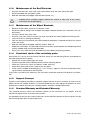
1
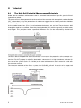
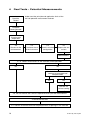
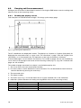
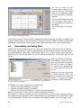
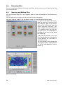
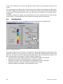
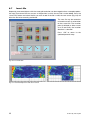
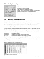
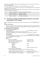
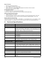
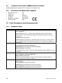
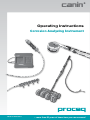
canin
+
Operating Instructions
Corrosion Analyzing Instrument
Made in Switzerland
... more than 50 years of know-how you can measure!
Table of Contents
1
1.1
Safety and Liability
General Information
4
4
1.2Liability
4
1.3
Safety Instructions
4
1.4
Symbols used in the operating instructions
4
1.5
Correct Usage
4
2Tutorial
5
2.1
The Half-Cell Potential Measurement Principle
5
2.2
Factors affecting the Potential Measurement
6
2.3
Application Limits of the Potential Measurement Technique
6
2.4
The Electrical Resistivity Measurement Principle
7
2.5
Influence of Rebars on Electrical Resisitivity Measurements
7
2.6
Effect of Electrical Resistivity on Half-cell Potential Measurements
7
3
Getting Started
8
3.1
Prepare the electrode(s)
8
3.2
Connect the electrode / probe to the indicating device
8
3.3
Power ON and select the correct operating mode
3.4
Functional check of the equipment
4
Real Tests – Potential Measurements
9
10
10
4.1
Planning and preparation
11
4.2
Selecting the correct grid
11
4.3
Choosing the appropriate electrode
11
4.4
Connect to the reinforcement
11
4.5
Functional check of the instrument
11
4.6
Preparation of the test surface
12
4.7
Check to see if coatings need to be removed
12
4.8
Pre-moistening the concrete surface
12
4.9 Carrying out the measurement
4.9.1
Reading the display screen
4.9.2
Measuring with the Rod Electrode
4.9.3
Measuring with the Wheel Electrode
4.9.4
Re-opening an object
4.9.5
Overwriting or deleting readings
4.10Evaluation
4.10.1 Example of a typical distribution
4.11 Confirmation and refining of hotspot positions
13
13
14
15
15
15
16
16
17
5
General Settings
17
5.1Backlight
17
5.2
Navigating around the menus
17
5.3
Selecting the operating mode
18
5.4
Configuring the instrument for potential measurement (See Fig 5.1)
20
5.5
Configuring the instrument for electrical resisitivity measurement (See Fig 5.2)
21
6
CANIN ProVista Software
21
6.1
Installing CANIN ProVista
21
6.2
Starting CANIN ProVista
21
6.3
Downloading and Saving Data 22
6.4
Renaming Files 23
6.5
Opening and Editing Files 23
6.6Configuration
24
6.7
25
Insert file
6.8Edit
26
6.9
26
Additional Functions
6.10 Relative frequency
27
6.11 Cumulative frequency
27
6.12 Chipping graph
28
6.13Annotations
28
7
Measuring the electrical resistivity
29
7.1
Preparing the concrete surface for measurement
29
7.2
Reading the display screen
30
7.3
Measuring with the Wenner Probe
30
8.
Transfer of Electrical Resisitivity Data to a PC (Windows 2000 / XP / Vista)
31
9
32
Technical Specifications
9.1
Technical Information CANIN ProVista software
33
9.2
Standards and Regulations Applied
33
10
Part Numbers and Accessories
33
10.1 Complete Units
33
10.2Accessories
34
11
Maintenance and Support
34
11.1 Functional check of the electrodes
34
11.2 Maintenance of the Rod Electrode
35
11.3 Maintenance of the Wheel Electrode
35
11.4 Functional check of the resistivity probe
35
11.5 Support Concept
35
11.6 Standard Warranty and Extended Warranty
35
1
Safety and Liability
1.1
General Information
This manual contains important information on the safety, use and maintenance of the Canin+. Read
through the manual carefully before the first use of the instrument. Keep the manual in a safe place
for future reference.
1.2Liability
Our “General Terms and Conditions of Sales and Delivery” apply in all cases. Warranty and liability
claims arising from personal injury and damage to property cannot be upheld if they are due to one
or more of the following causes:
•
•
Failure to use the instrument in accordance with its designated use as described in this manual.
Incorrect performance check for operation and maintenance of the instrument and its components.
• Failure to adhere to the sections of the manual dealing with the performance check, operation
and maintenance of the instrument and its components.
• Unauthorised modifications to the instrument and its components.
• Serious damage resulting from the effects of foreign bodies, accidents, vandalism and force
majeure
All information contained in this documentation is presented in good faith and believed to be correct.
Proceq SA makes no warranties and excludes all liability as to the completeness and/or accuracy
of the information.
1.3
Safety Instructions
The equipment is not allowed to be operated by children or anyone under the influence of alcohol,
drugs or pharmaceutical preparations. Anyone who is not familiar with this manual must be supervised when using the equipment.
•
•
•
Carry out the stipulated maintenance properly and at the correct time.
Following completion of the maintenance tasks, perform a functional check.
Pay attention to the correct use and disposal of the copper sulphate solution and the cleaning
material.
1.4
Symbols used in the operating instructions
Danger!: This symbol indicates a risk of serious or fatal injury in the event that certain rules of behaviour are disregarded
i
Note: This symbol indicates important information
1.5
•
Correct Usage
•
•
The instrument is only to be used to determine the corrosion potential of rebars in concrete or the
electrical resistance of concrete.
Replace faulty components only with original replacement parts from Proceq.
Accessories should only be installed or connected to the instrument if they are expressly authorized by Proceq. If other accessories are installed or connected to the instrument then Proceq will
accept no liability and the product guarantee is forfeit.
4
© 2012 by Proceq SA
2Tutorial
2.1
The Half-Cell Potential Measurement Principle
Under normal conditions reinforcement steel is protected from corrosion by a thin, passive film of
hydrated iron oxide.
This passive film is decomposed due to the reaction of the concrete with atmospheric carbon dioxide
(CO2, carbonation), or by the penetration of substances aggressive to steel, in particular chlorides
from de-icing salt or salt water.
At the anode ferrous ions (Fe++) are dissolved and electrons are set free. These electrons drift
through the steel to the cathode, where they form hydroxide (OH-) with the generally available water
and oxygen. This principle creates a potential difference that can be measured by the half-cell
method.
The basic idea of the potential field measurement is to measure the potentials at the concrete surface, in order to get a characteristic picture of the state of corrosion of the steel surface within the
concrete. For this purpose a reference electrode is connected via a high-impedance voltmeter (in
the case of the system Canin+ R = 10 MΩ) to the steel reinforcement and is moved in a grid over
the concrete surface.
The reference electrode of the Canin+ system is a Cu/CuSO4 half-cell. It consists of a copper rod
immersed in a saturated copper sulphate solution, which maintains a constant, known potential.
5
© 2012 by Proceq SA
Typical orders of magnitude (for information only) for the half-cell potential of steel in concrete measured against a Cu/CuSO4- reference electrode are in the following range (RILEM TC 154-EMC):
•
•
•
•
•
•
water saturated concrete without O2: moist, chloride contaminated concrete: moist, chloride free concrete: moist, carbonated concrete: dry, carbonated concrete: dry, non-carbonated concrete: 2.2
-1000 to -900 mV
-600 to -400 mV
-200 to +100 mV
-400 to +100 mV
0 to +200 mV
0 to +200 mV
Factors affecting the Potential Measurement
Provided that the corrosion conditions are equal (chloride content or carbonation of the concrete at
the steel surface) the main influences upon the half-cell potentials are:
Moisture
See the figures above for moist, carbonated concrete and dry, carbonated concrete. Moisture has a
large effect on the measured potential leading to more negative values.
Temperature
In order to measure the potential there must be a contact between the probe and the electrolytes in
the pore system of the concrete. Therefore a measurement below the freezing point is not recommended and can lead to incorrect readings.
Concrete cover thickness (Measure with Profometer / Profoscope)
The potential that can be measured at the surface becomes more positive with increasing concrete
cover. Variations in the concrete cover can cause deviations in the measurements. Very low concrete
cover can lead to more negative potentials which would seem to indicate high levels of corrosion.
Therefore it is advisable to make concrete cover measurements along with the half-cell measurements.
Electrical resistivity of the concrete cover (Measure with the Wenner Probe)
This topic is dealt with in detail in section 2.4
Oxygen content at the reinforcement
With decreasing oxygen concentration and increasing pH-value at a steel surface its potential
becomes more negative. In certain cases of concrete components with a high degree of water saturation, low porosity and/or very high concrete cover and thus low oxygen supply, the potential at the
steel surface may be very negative even though no active corrosion is taking place. Without checking
the actual corrosion state this may lead to misinterpretation of the potential data.
The air permeability of the concrete may be tested with Proceq’s Torrent instrument.
2.3
Application Limits of the Potential Measurement Technique
The potential field measurement even with a coarse grid delivers good results for chloride induced
corrosion. This type of corrosion is typified by pitting developing into troughs. This strongly affects
the diameter of the reinforcement and thereby greatly affects the load bearing capacity. Corrosion
due to carbonation is typified by the development of smaller macro-elements and is only possible to
determine by using a very fine grid if at all.
Corrosion of pre-stressed steel reinforcement is not possible to detect if it is located within a protective tube.
The potential field measurement alone offers no quantitative conclusions about the rate of corrosion.
Empirical studies have shown that there is a direct relationship between the corrosion rate and the
electrical resisitivity. However corrosion rate readings are of limited value as the rebar corrosion rate
varies considerably with time. It is more reliable to work with corrosion readings taken over a period
of time.
6
© 2012 by Proceq SA
2.4
The Electrical Resistivity Measurement Principle
As we have seen above, corrosion is an electro-chemical process. The flow of the ions between the
anodic and cathodic areas and therefore the rate at which corrosion can occur is affected by the
resistivity of the concrete.
The Wenner Probe is used to measure the electrical resistivity of the concrete. A current is applied to
the two outer probes and the potential difference is measured between the two inner probes.
I
Resistivity ρ= 2πaV/l [kΩcm]
V
a
a
a
Empirical tests have arrived at the following threshold values which can be used to determine the likelihood of corrosion.
When ρ ≥ 12 kΩcm corrosion is unlikely
When ρ = 8 to 12 kΩcm corrosion is possible
When ρ ≤ 8 kΩcm corrosion is fairly certain
The electrical resistivity of the concrete cover layer decreases due to:
• increasing concrete water content
• increasing concrete porosity
• increasing temperature
• increasing chloride content
• decreasing carbonation depth
When the electrical resistivity of the concrete is low, the rate of corrosion increases.
When the electrical resisitivity is high, e.g. in case of dry and carbonated concrete, the rate of corrosion decreases.
2.5
Influence of Rebars on Electrical Resisitivity Measurements
The presence of rebars disturbs electrical resisitivity measurements as they conduct current much
better than the surrounding concrete. This is particularly the case when the cover depth is less than
30mm. In order to minimize the effect, none of the electrodes should be placed above a rebar when
measuring, or if this is unavoidable, then perpendicular to the rebar.
2.6
Effect of Electrical Resistivity on Half-cell Potential Measurements
Low electrical resistivity leads to more negative potentials that can be measured on the surface and
the potential gradients become flatter.
In this case the measurement grid for potential measurements may be coarser, as the risk of undetected anodic areas with flatter gradients becomes lower. However, as the resolution between corroding and passive areas is reduced, this may lead to an overestimation of the actively corroding
surface area.
High electrical resisitivity leads to more positive potentials that may be measured on the surface and
potential gradients become steeper.
In this case the measuring grid must be made finer, in order to be able to locate an anode with a
very steep gradient. However, the more potentials may be misinterpreted as passive areas when only
considering the absolute value of the potential.
7
© 2012 by Proceq SA
3
i
3.1
Getting Started
Note: First time user: Complete the tutorial OR see a demo by a qualified Proceq
representative.
Prepare the electrode(s)
Rod Electrode - Before filling, remove the cap with the wooden plug and soak it in water for about
an hour to allow the wood to saturate and swell.
Wheel Electrode - The wooden plug is not intended to be removed. Immerse the wheel in water
well before you intend to use it to allow water to soak into the plug. The felt hoops and the felt hoop
connector should be saturated with water before measuring.
Copper Sulphate (Rod and Wheel) - Prepare the saturated solution by mixing 40 units by weight
of copper sulphate with 100 units by weight of distilled water. In order to ensure that the solution
remains saturated, add an additional teaspoonful of copper sulphate crystals into the electrode.
The electrode should be filled as completely as possible with a minimum of air in the compartment. This ensures that the solution is in contact with the wooden plug even when measuring in an
upwards direction.
Caution! When handling copper sulphate be careful to take note of the safety
instructions on the packaging.
3.2
Connect the electrode / probe to the indicating device
Connect the half-cell electrode or Wenner Probe to the device as shown below:
Rod electrode connects to INPUT A and also
requires GND connection.
Wheel electrode connects to INPUT A, path
measurement connects to INPUT B.
GND connection is also required. (See 4.4)
Wenner probe connects to INTERFACE
RS232C only.
8
© 2012 by Proceq SA
3.3
Power ON and select the correct operating mode
Press the ON/OFF button to power on.
The indicating device has two distinct modes of operation:•
•
Corrosion analysing
Electrical resistivity meter
It will start up in whichever mode was
used last. For potential measurements the
instrument must be in “Corrosion analysing” mode.
Switch between modes by pressing MENU,
place the cursor at “Wenner Probe”,
press START, select “OFF” for Corrosion
Analysing” mode or “ON” for Resistivity
Meter. (See 5.3) Press MENU or END.
3.4
Functional check of the equipment
Perform a functional check of the equipment as described in sections 4.5 and 11.
Congratulations! Your Canin+ is fully operational and you can now start your measurements.
9
© 2012 by Proceq SA
4
Real Tests – Potential Measurements
2
Read the
Tutorial
Understand the principle and application limits of the
half cell potential measurement method.
3
Complete
Getting Started
4.1
Planning and
preparation
4.4
Connect to the
reinforcement
4.5
Functional check
of the instrument
5.4
Check instrument
configuration
4.6
Prepare the test
surface
Measurement
4.7 Is a direct measurement on the concrete surface possible?
Yes
No
Can the influence from surface
coatings be estimated and
compensated?
Yes
No
Remove the
surface coating
4.8, 4.9 Pre-moisten the surface if required and carry out the measurement
4.10 Evaluate the data
4.11 Confirm and refine corrosion hotspot positions at openings in the concrete
10
© 2012 by Proceq SA
4.1
Planning and preparation
In Canin+, the measurement data is stored in files called “Objects”. In order to make the evaluation
simpler it is recommended before beginning work to map out the site and assign various sections to
particular “Objects”. This will facilitate the evaluation in ProVista at a later stage.
In order to minimize the effort needed for the investigation, the site can be divided into sections that
are subjected to similar amounts of wear, by means of a visual inspection. (e.g. Multi-story car park:
Entrance area, traffic lane, parking areas, areas with and without cracks or obvious areas where
puddles form.) Following this inspection, representative sub-sections should be chosen, in which the
potential field measurements are carried out with the Canin+ system.
4.2
Selecting the correct grid
One method is to use a relatively large grid for a first estimate, e.g. 0.50 x 0.50 m2 up to a max of 1.0
x 1.0 m2 using the coarse grid. (See 5.4).
Suspect areas can be further investigated using a finer grid (e.g. 0.15 x 0.15 m2), to identify as closely
as possible the extent of the surface that will require corrective maintenance.
Vertical elements usually require a smaller grid (e.g. 0.15 x 0.15 m2). The same applies to slender
elements, for which the grid will be defined by the geometry, (e.g. steps, beams and joints etc.).
For large horizontal surfaces (parking decks, bridge decks etc.) a grid of 0.25 x 0.25 m2 to 0.5 x
0.5m2 is typically sufficient.
4.3
Choosing the appropriate electrode
Depending on the surface under test, it is necessary to choose which type of electrode will be
employed. For small areas or areas that are difficult to access, the small and light Rod Electrode will
typically be used. For more accessible horizontal, vertical or overhead surfaces, it is much faster to
use the 1-Wheel Electrode. For large horizontal surfaces the 4-Wheel Electrode is recommended for
the reason of the significantly faster automatic measurement in a pre-defined grid.
4.4
Connect to the reinforcement
The ground cable must be connected to the reinforcement of the surface to be measured. This is
usually done by chiseling or drilling to the reinforcement. In some cases it may be possible to use
existing building elements that are connected to the reinforcement (e.g. water pipes, earth points).
The connection to the reinforcement should be made with the least possible resistance. To this end
it may be beneficial to grind the reinforcement with (e.g using an angle grinder) and to connect the
cable with welding tongs.
The connection should be tested for continuity. This requires at least one other point of the reinforcement to be exposed and to check the resistance between the two with an Ohmmeter. The connections should be situated as far as possible in opposing corner areas of the surface under test. The
measured resistance should not be more than 1 Ω above the resistance of the cable used.
4.5
Functional check of the instrument
Before real tests begin, a functional check is recommended (see section 11).
Additionally the probes should provide a stable value close to zero (typically E = ± 20 mV) when they
are held in the air and the Canin+ instrument is connected to earth.
It is also a good idea to make comparison measurements on areas that are clearly damaged against
areas that are clearly intact. (e.g. at the base of a column with obvious corrosion compared with
columns at a height of approximately 1.50 m without any visual damage.) Here also stable values
should be obtained, whereby the measured values in the damaged area should be significantly more
negative than the values from the undamaged area.
11
© 2012 by Proceq SA
If the results obtained are doubtful, then it is often the case that there is a contact problem, e.g.
connection to the reinforcement or the connection between the probe and the Canin+-instrument,
respectively inadequate preparation of the probe (copper sulphate solution). Furthermore it is possible that a film of water on the probe or telescopic extension can create an electrical connection to
the person carrying out the measurement. This can also affect the results. These error sources are
easily corrected and the check should be repeated.
Check the instrument configuration (See 5.4).
4.6
Preparation of the test surface
It is recommended to mark out a grid on the surface corresponding to the grid you wish to use. For
small areas where point measurements will be made with the Rod Electrode this can be done by
using a tape or by drawing the grid on the element. For large areas such as parking and bridge decks
the wheel electrode is preferable. The integrated path measurement ensures the correct grid in the
direction of measurement. To ensure the correct grid between parallel measurement paths marks
can be drawn on the surface. Please note the 4-Wheel Electrode ensures a stable parallel grid and
requires less marks to be drawn on the surface.
4.7
Check to see if coatings need to be removed
It is not possible to make a measurement through an electrically isolating coating (e.g. an epoxy resin
coating, sealing sheets or asphalt layers.)
It is possible to make a measurement through thin dispersion coatings, that are often used, for
example on the walls and ceiling of underground car parks, however this can cause a small shift of
the potentials.
It is always necessary to check whether or not a measurement can be made through a coating.
To do this, potentials should be measured at a few locations
• in the first place through the coating and
• with the coating removed
If possible areas with largely varying potentials should be chosen. If there is no alteration of the
potential, or if a shift of the potential can be compensated by a correction (e.g. ΔE = ± 50 mV), then
a measurement can be made directly on the coating. If not, then the coating must be removed before
making the measurement.
4.8
Pre-moistening the concrete surface
The contact between the pore solution of the concrete and the probe can be impaired by a dried out
concrete skin. This can greatly increases the electrical resisitivity of the concrete.
It is therefore recommended to moisten the surface approximately 10 to 20 minutes before carrying
out the measurement.
If this is not possible, it must be ensured that the sponge on the Rod Electrode or the felt hoops
on the wheel electrode are sufficiently moistened. In this case, when making a measurement, the
probe must be held against the surface until a stable end value is reached. (If the surface is dry at
the beginning of the measurement, it has to be moistened by the sponge on the probe so a stable
value will not be present initially.)
This is only possible with the Rod Electrode.
In the case of the wheel electrode with its continual automatic measurement, it is not possible to
monitor whether or not the measured value is stable. Therefore it is recommended to pre-moisten
the surface section wise and to measure in intervals of a few minutes.
12
© 2012 by Proceq SA
4.9
Carrying out the measurement
Configure your instrument as described in section 5. Pressing the END button saves the settings and
takes the user to the measuring screen.
4.9.1
Reading the display screen
From here press the START button to begin. This brings up the empty page.
Fig 4.1 Page with a grid of 150/150 mm.
The XY- coordinates are displayed in meters. The display has 16 points x 15 points (240 points) for
displaying the measured values as a grey scale. This constitutes a “page”. With the XY-grid set to
150/150mm, as in the example here, this represents a total area of (2250mm x 2100mm).
A total of 980 pages can be stored in the memory. The number of pages that are still available for
use is shown in the top right hand corner of the measuring screen (Fig 5.1). (e.g. 491 P indicates 491
pages are still available.)
The number of pages contained in an object is not limited except by this.
1 – The cursor shows the next measurement location
2 – The arrow shows in which direction the cursor will move. This can be altered to match the measurement direction by pressing the arrow keys.
3 – The measured value.
4 – The Object number.
5 – The meter value. E.g. a 10 will be shown here if we have travelled 10m in the X-direction.
6 – Indications (Switch between the two by pressing MENU whilst in the measuring screen):
Indicator
r
R
*
-
13
Probe type
Rod Electrode
Rod Electrode
Wheel Electrode
Wheel Electrode
Indication
XY-grid
coarse grid
Measurements will be automatically overwritten
Measurements will not be overwritten
© 2012 by Proceq SA
4.9.2
Measuring with the Rod Electrode
The cursor begins in the top left hand corner of the XY-Grid (Fig 4.1). This indicates where the first
measurement will be stored, so it is important to take the first measurement in the corresponding
point marked on the concrete.
i
•
Note: The first measurement must not necessarily be made in the top left hand
corner. Before making any measurement, you may move the cursor around on the
screen using the ↑↓← → buttons to the desired location. This is particularly useful
if there is some kind of obstruction on the test object which means that a measurement cannot be made in that position. By moving the cursor as described you can
move on the grid to clear the obstruction and continue measuring. The important
thing is that your position on the screen should match the actual position on the
concrete.
Moisten the foam rubber plug of the electrode with water and press it lightly onto the first measuring point. The measured value will be shown in mV in the centre of the display. Once it stabilizes, a beep will indicate when the measurement has been acquired automatically. (See 5.4). At
this point the mV value is blended out and a grey scale indication will be placed on the grid. The
cursor will move to the next point to be measured.
Following the measurement it should be possible to see a wet patch when applied on dry concrete. If this is not the case then the foam rubber plug should be moistened with water again.
The simplest way to proceed is to make the measurements as proposed by the instrument. i.e.
begin in the top left hand corner and move along the row in the X-direction according to the
column width, e.g. 150mm between measuring points.
When you come to the end of a row, you must press the ↓ button to indicate this and the cursor
will jump down to the next row. The direction arrow (Field 2 in fig 4.1) will automatically change
direction to ←.
Now you can proceed to measure in the opposite direction along this row. When the end is
reached, i.e. you are back at the Y-axis, the cursor will automatically jump down to the next row
and the direction arrow will change back to →.
When you come to the end of a page the cursor automatically jumps to the next page.
•
•
•
•
•
i
Note: The instrument can also be used to measure along the Y-axis, i.e. up and down
the columns. This is done by altering the direction arrow to ↓ before starting. In this
case you must indicate to the instrument that you have reached the end of a column
by pressing the → button.
i
Note: The PRINT button can be used to mark an “X” on the display in the place of a
measurement value. This is useful for marking the position of cracks etc.
When you have finished making all of the measurements you require on the concrete press the END
button. The measured values are stored automatically.
14
© 2012 by Proceq SA
4.9.3
Measuring with the Wheel Electrode
As described in 4.9.2, begin at the location corresponding to the top left hand corner of the screen
and move in the direction indicated or alter this accordingly.
•
•
Press the START button to acquire the first reading.
Now proceed to move the wheel electrode in the Y-direction (down) as indicated by the direction
arrow (Field 2 in fig 4.1). The measurement readings will be acquired automatically in the preselected row spacing.
When you come to the end of a column, press the → button to indicate this and the cursor will
jump right to the next column. The direction arrow will automatically change direction to ↑.
Now place the wheel physically one column spacing to the right and acquire the first measurement by pressing the START button. Proceed to measure back along the Y-axis (up) as indicated
by the direction arrow.
When you come to the end of the measurement surface, (the X-axis) the cursor will automatically
jump to the next column and the direction arrow will change back to ↓.
Following each manual or automatic change in the direction arrow, the path measurement and
the automatic acquisition of the potential reading is halted.
These breaks in the measurement process can be used for example to refill the water compartment. Automatic measurement begins again when the START button is pressed.
During such breaks, the measured value is shown in the status row. (Field 3 in Fig 4.1)
The maximum speed of travel should not exceed a maximum of 1m/sec.
Measurements along the X-axis cannot be acquired. (Objects may be rotated later in ProVista)
•
•
•
•
•
•
•
•
i
Note: The nozzle (Ø 1 mm) is fit as standard. On dry surfaces, the felt hoop should
leave a clearly visible trace as you measure. Depending on the character of the
concrete it may be necessary to increase to one of the larger nozzle diameters (Ø
2 or 3 mm).
i
Note: On dry, vertical surfaces, measurements should be made downwards as this
ensures an even moistening of the surface.
4.9.4
Re-opening an object
An object can be re-opened and missing measurements can be entered or suspect measurements
can be overwritten. However the following points should be observed.
Once an object has been closed and a new object has been opened, it is no longer possible to add
pages to a previously opened object.
If you have worked out the size of the area assigned to an object (see 4.1), it is possible to reserve
the number of pages you will require in the case that you are not able to complete the measurement
in one go.
A page is reserved once it has appeared on the screen. In order to reserve the necessary pages,
simply move the cursor to each page you will require. For a better orientation it may help to place an
“X” (see Note in 4.9.2) somewhere on the page (but not in the top left hand corner).
The last object that was opened can be re-opened and extended at any time.
4.9.5
Overwriting or deleting readings
Existing readings can be overwritten by moving the cursor to the appropriate point and making a
new reading with the electrode. Once the reading has registered, the cursor will move to the next
measuring point along the axis indicated by the direction arrow.
To delete an existing reading, move the cursor to the point you wish to delete and press PRINT for
two seconds. Once the reading has been deleted, the cursor will move to the next measuring point
along the axis indicated by the direction arrow.
15
© 2012 by Proceq SA
4.10Evaluation
Typically, two criteria must be considered for the evaluation. (This is merely a guideline. The actual
evaluation should be carried out by a corrosion engineer.)
1.
Active corrosion can be expected at locations where a negative potential is surrounded by
increasingly positive potentials, i.e. locations with a positive potential gradient. Potential differences with delta of around +100mV within a 1m measurement area, together with negative
potentials are a clear indication of active corrosion.
2.
In order to plan corrective maintenance it is necessary to draw a border between areas of
active corrosion (anodes) and passive areas (cathodes) within the surfaces showing potential
gradients. In order to do this it is necessary to set a threshold potential that defines the intersection between the two states. ProVista has functionality which aids in this. (Read section 6
for details).
4.10.1 Example of a typical distribution
If the surface under test has both actively corroding as well as passive rebars, then the two states
exhibit differing statistical distributions of the potential. In the graphical representations provided
by ProVista there are typically three characteristic sections (Fig. 4.2). A flattening out of the section
shows that in these value ranges, there is less data available, i.e. the boundaries of the distribution
are here.
Fig. 4.2 Example of a relative frequency chart and cumulative frequency chart.
The potential ranges of active corrosion and passivity overlap.
The red cursor (leftmost) = minimum of the passive distribution.
The yellow cursor (rightmost) = maximum of the active distribution.
Active corrosion is practically certain in the region of the left hand (more negative) straight section.
Once these cursor lines have been set, the surfaces in this potential range will be automatically
displayed in the corresponding colour in the CANIN ProVista “Chipping Plot”.
In the example the red cursor line marks this threshold. A typical “Chipping Plot” taken from a practical example is shown below.
16
© 2012 by Proceq SA
The right hand side straight section almost certainly corresponds to passive reinforcement. This
is displayed automatically in the “Chipping Plot”
in green.
In the overlapping range active corrosion and
areas of passivity can be present with the same
potential values. Areas with potential values in
this area are displayed automatically in yellow in
the “Chipping Plot”. In this overlapping range it is
assumed that a definite statement on the corrosion state is not possible and such sub-sections
may only be evaluated by more extensive investigations.
4.11
Confirmation and refining of hotspot positions
Once the potentials have been evaluated, it is recommended to make openings in the concrete to
verify the threshold potential. Prior to making the opening it is recommended to locate the exact position of the reinforcement bars by means of a rebar locator (e.g. Proceq’s Profometer, Profoscope).
Moreover a fine measurement with the Rod Electrode using a small grid is recommended to determine the actual “Hotspot” (local potential minimum).
5
General Settings
5.1Backlight
The display has a back light which can be switched on or off by pressing the END button for more
than 2 seconds when the measurement screen is displayed. When the backlight is on, an asterisk is
shown in the top right hand corner.
5.2
Navigating around the menus
The diagrams in Fig 5.1 and Fig 5.2 show the menu structure for configuring the equipment for
potential measurement and electrical resisitivity measurement respectively. On start up, the measuring screen is shown. Press MENU to access the main menu for the mode selected.
For all the selected menus: Use the ↑↓ and ← → buttons to select menu items and adjust settings.
•
•
•
If the option START is indicated at the bottom of the screen, pressing this will take you to the
selected menu item.
Pressing MENU saves the settings and takes you back to the main menu.
Pressing END saves the settings and takes you to the measurement screen.
5.3
Selecting the operating mode
Wenner Probe – This menu item switches between operating modes.
For potential measurement it is OFF.
For resistivity measurement it is ON.
17
© 2012 by Proceq SA
Fig 5.1 Menu Overview for Potential Measuring
MENU
END
END
START
MENU
START
Use the ↑↓ and →←to select, navigate and adjust settings
Pressing END saves the settings and takes you to the measuring screen
Pressing MENU saves the settings and takes you to the next higher menu
END
MENU
END
18
© 2012 by Proceq SA
MENU
Main menu for resistivity measuring
ON
OFF
Fig. 5.2 Menu Overview for Resistivity Measuring
19
© 2012 by Proceq SA
END
MENU
START
END
END
START
OFF
MENU
ON
Main menu for potential measurement
Use the ↑↓ and →←to select, navigate and
adjust settings
Pressing END saves the settings and takes you
to the measuring screen
Pressing MENU saves the settings and takes
you to the next higher menu
END
MENU
MENU
5.4
Configuring the instrument for potential measurement (See Fig 5.1)
Display – The values determine the grey scale values that will be used on the screen. The total range
possible is between +200 and -950 mV. An optimal base setting is between -0 and -350 mV.
This range can be adjusted at any time later to make the display easier to read. It does not affect any
measurements made, only how they are displayed.
Object No. – Set the name for the “file” where the current measurement data will be stored.
i
Note: Object No. 1 is a Demo-Object consisting of 6 pages of data, which can be
edited. However, when the instrument is switched off and on, the original values will
be restored.
Language – The language is valid for both potential and resistivity modes.
Electrodes – Set Way Encoder to “Yes” for the wheel electrode and “No” for the Rod Electrode.
Select the number of electrodes, typically 1 for the Rod Electrode and 1 or 4 for the wheel electrode.
The option Automatic Measuring is for the Rod Electrode only. The wheel electrode always measures
automatically.
i
Note: If automatic measuring is selected, then measured values of < -50mV will be
acquired automatically once the value has stabilized. If automatic measuring is not
selected then values have to be acquired by pressing the START button. In both
cases, values between +200 and -50mV have to be acquired by pressing the START
button.
XY-Grid – Define the scale of the measurement grid.
i
Note: The XY-Grid values can only be altered if a new “Object” has been defined. If
an Object already contains measurements, then it is no longer possible to change
the grid.
i
Note: X and Y must be equal if you wish to export the data to ProVista
Coarse Grid – Define how many times the coarse grid is larger than the XY-Grid already defined.
Example: when distance between measurement points in the XY-Grid is set to 150 mm and the
number of steps in the coarse grid is set to 5, the distance between measurement points in the
coarse grid is 5x 150 = 750mm. This is useful for carrying out an initial sweep and switching to a fine
grid for detailed investigations. (See 4.2)
i
Note: When the equipment is switched off, the coarse grid number of steps is reset
to “1”.
Data Output – Used to clear the memory and re-open objects for display. Data transfer to a PC is
handled by CANIN ProVista (See 6.3).
Clear Memory erases all of the stored measurements for the active mode. It is not possible to delete
single objects. Once this has been confirmed, it is not possible to undo the action. The objects for
the other mode are unaffected.
20
© 2012 by Proceq SA
5.5
Configuring the instrument for electrical resisitivity measurement (See Fig 5.2)
Most of the screens are identical to the potential mode and have been explained there.
Device Constants – Enter the 3-digit code engraved on the resistivity probe. (See 11.4)
Data Output – Used to clear the memory and re-open objects for display as in 5.4. In this mode also
used to export data to a PC. Select the Object you wish to export. Press the END button to open
the measuring screen where the main information of this object will be displayed. Transfer the data
to the PC using Hyperterminal as described in section 8.
6
CANIN ProVista Software
The CANIN ProVista software enables the data transfer, the graphical presentation of the potential
fields and a statistical analysis of the measurement data collected and stored on the Canin+. In addition, CANIN ProVista allows the automatic derivation of a chipping plot for concrete replacement.
These graphs can be inserted in an assessment report and serve the corrosion engineer together
with results of non-destructive and destructive tests like concrete cover depth, carbonation depth,
chloride profile etc. as basis for interpretation of his results.
The programme does not state the condition of the concrete structure, e.g. severity of corrosion of
the rebars and it cannot propose the remedial actions. The engineer must be able to interpret all
measured values in order to propose the necessary actions.
Additionally all graphics can be exported for editing in drawing programs and thereby inserted into
plans for the execution of repair measures.
6.1
Installing CANIN ProVista
Locate the file “CaninInstallerx.xx.zip” file provided on the data carrier. Unzip the file and open the
folder called “Volume”.
Locate the file “setup.exe” and click on it.
Follow the instructions you see on the screen. This will install CANIN
ProVista on your PC. It will also create a desktop icon for launching the
program.
6.2
Starting CANIN ProVista
Either click on the desktop icon or click on the CaninProVista entry in the
“Start” menu. “Start – Programs – CaninProVista”.
21
© 2012 by Proceq SA
The user can insert his own
company logo by placing a bitmap file with the name Logo.
bmp in the Configuration folder
in the CaninProVista installation
directory.
The size of the bitmap has to be
210 x 50 pixels. From there it
will automatically be copied into
the graphs.
The Proceq logo is unchangeable.
Fig. 6.1: Canin ProVista Main Window
There are four sections. The top contains labelling information including a user logo, the middle is the
graphical representation of the measurement, the bottom contains additional numerical information
regarding the measurement and the graph, and the right hand side contains the navigation pane.
6.3
Downloading and Saving Data
Connect the indicating device to your PC using the transfer cable (330 00 456) and the RS-232 –
USB adaptor (390 00 542). In order to download data, the Data Output submenu must be visible on
the indicating device. Select Menu “Data Output” (Fig 5.2) in the Canin+ display device and press
START. Click on VistaTransfer button to start the download programme. A dialog box appears (see
Fig. 6.2).
Select the respective COM port.
All the objects stored in the display unit are listed in the field on
the left. By default, all objects
are selected for downloading,
i.e. all the check boxes contain
a cross.
Especially If you are using a USB
to Serial converter make sure
that a COM port from COM1 to
COM4 is assigned. All higher
COM ports are not supported.
Fig. 6.2: VistaTransfer Window
If the object list is empty, please check the following:
• Whether the correct COM port is selected.
• Whether the cable is properly connected.
• Whether the Data Output submenu is visible on the indicating device.
Click the check boxes to select and de-select the individual list entries.
Use “Browse” to select the location you wish to store the data. Click the “Save selected” button to
start the downloading procedure. The PC downloads all the selected objects and stores them as files
in the selected folder. The file names are identical to the object numbers and the file type is PVO.
22
© 2012 by Proceq SA
6.4
Renaming Files
You can use Windows Explorer to rename stored files. Any file names can be used. The file type
must always be PVO.
6.5
Opening and Editing Files
Click on the button Open File in the navigation pane and select the desired file in the Window that
appears.
Files of type pvo or bin are the only files that Canin ProVista recognizes.
If the file is valid, the window in Fig. 6.3 appears asking you for the desired rotation/mirroring.
It may be that the objects from a complete site were not all measured in the
same direction. (See 4.9.3). ProVista
allows this to be corrected. Select the
correct orientation and press “OK”
again to display the measurement file
as a potential map in the main window (see Fig. 6.4). If the selected file is
invalid for any reason a warning dialog
box will pop up.
To be valid, the grid that is set in the
Canin+ display device must be equal in
x-and y-direction, e.g. 150x150mm or
305x305mm (1x1ft).
The Canin+ display device accepts the
unit length [mm] only. CANIN ProVista
can convert and display the scale of
length in ft.
Fig. 6.3: Orientation selection window
Fig. 6.4: Potential Map
23
© 2012 by Proceq SA
A title, short comment, the name of the operator and the date can be entered at the top of the
screen.
The scale represents the dimensions in either meters or feet. (See 6.6) The legend to the right shows
the colour coding of the measurement values (in millivolts) and the number of measurement points
in each range. The three fields Xmax, Xmin, Ymin allow the user to zoom in on a particular area in
the graph.
The bottom section of the window shows the positions for cursors A and B and the mV value of their
current position. The grid direction values indicate the resolution of the measurement.
6.6Configuration
Click on “Configuration” to alter the appearance and the language of the potential map.
Fig. 6.5: Configuration Window
The number range to which the colours are assigned can be changed through varying the base value
and delta. The base value may not be any smaller than -999 and the combination of the base value
delta may not lead to any colour representing anything above 1000 mV. By pressing “Default”, the
base value and delta are changed to -400mV and 50mV respectively.
•
•
•
•
•
24
Left clicking on a colour allows the colour for that particular range to be selected.
Warnings for overwriting and deleting values in a graph can be set.
Set imperial or metric units for the display with the drop down menu “Unit length”.
“Diagram Orientation” allows the origin of the graph to be changed.
Set the language of the program with the drop down menu.
© 2012 by Proceq SA
6.7
Insert file
Separately measured objects with the same grid resolution can be merged to form a complete potential map. Place one of the two cursors at the position in which the new file is to be added. Press the
“Insert File” button and select the file you wish to add. If the file is valid, the next screen (Fig. 6.6) will
allow the file to be correctly positioned.
The new file may be rotated or
mirrored to match its orientation
to the current file. The insertion
point is defined as either cursor
A or B and finally the insertion
direction is selected.
Press “OK” to return to the
updated potential map.
Fig. 6.6: Insert Window
Fig. 6.7: Potential Map before and after Insertion
25
© 2012 by Proceq SA
6.8Edit
Individual values and sections of the potential graph may be edited.
Fig. 6.7: Edit graph screen
Use the A and B cursors to select the values to be edited. Press “Edit”. Four actions are available.
•
•
•
•
Delete the values lying in the area between cursors A and B.
Set the values lying in the area between A and B to a specific value.
Delete the value to the bottom right of cursor A.
Set the value to the bottom right of cursor A to a specific value.
6.9
•
•
•
•
•
•
26
Additional Functions
“Save File” to save your changes.
“Print View” prints the currently visible section of the potential map respectively chipping graph.
“Print File” prints the entire measurement file, even areas that are not visible in the current view
of the potential map/chipping graph, using as many pages as necessary.
“Get BMP” creates a BMP image file of the current view of the potential map or chipping graph
which can be exported to third party software for reporting.
“General View” resets the range of the potential map and chipping graph so that the entire graph
is visible again.
“Undo” allows the last 10 edits and insertions to be undone.
© 2012 by Proceq SA
6.10
Relative frequency
With the relative frequency function, a bar graph (as show in Fig.
6.8) of the measurement data is
created. The width of the bars
represents the measurement
range while the height of the
bar represents the relative frequency of measurements points
within that range. The range of
the graph can be changed by
entering the desired minimum
and maximum values in the
respective fields on the x-axis.
The limits are -1000 to +1000
mV. The class width can also be
changed.
Fig. 6.8: Relative frequency diagram
6.11
Cumulative frequency
Fig. 6.9: Cumulative frequency diagram
Following an evaluation (See 4.10), the corrosion engineer can place the 3 cursors in such a way that
they represent areas of different corrosion degrees.
They determine the colour distribution in the chipping graph.
It is possible to overlay two or even all three cursors and thereby decrease the number of divisions.
The cumulative frequency needs to be activated at least once for a newly opened file in order to be
able to view the chipping graph.
The range of the cumulative frequency graph can be changed by entering the desired minimum and
maximum values in the respective fields on the x-axis. The limits are -1000 to +1000 mV. The class
width can also be changed.
27
© 2012 by Proceq SA
6.12
Chipping graph
After having accessed the cumulative frequency graph, the “Potential Map” button becomes active.
By clicking on it, the visualization switches to the chipping graph (see Fig. 6.10).
The four colour regions of the chipping graph are based upon the three cursor positions in the
cumulative frequency graph.
These positions represent potential limits identified by the engineer as areas of equal condition where
the concrete has to be chipped to a certain depth for repair purposes.
Fig. 6.10: Chipping graph
6.13Annotations
Information about the concrete structure like measured chloride content, cracks or other defects
can be placed directly in the potential map or the chipping graph. The information will be printed
and shown in bitmaps.
By default they are created with an arrow that can be moved to point at a specific spot in the graph.
Annotations can be added by right clicking on the potential map or chipping graph and selecting
“Create Annotation”.
Fig. 6.11: Annotation window Fig. 6.12: Annotation Attributes
Right click on an annotation to select its attributes. If the Lock Name attribute is not selected, the
entire annotation (point, label and arrow) can be moved by left clicking on the annotation and dragging it around. If the Lock Name attribute is selected, the name will stay fixed and only the annotation
point with the arrow can be moved.
28
© 2012 by Proceq SA
i
Note: Always deselect the Lock Name attribute once an attribute is placed at the
proper position and before any print, BMP, or display change functions are used
(see Fig. 9.16).
i
Note: After having added annotations (see section Annotations) to a graph, changing the units length will cause the annotations to be misplaced. Therefore, before
adding annotations, ensure that the graph has the desired units.
Once you have added annotations, it is recommended that the file is saved. The dimensions of the
graph or the colour scale can then be changed. When changes to the dimensions of the graph are
relatively large, it can occur that label location of the annotation will move. To restore the annotations
correctly, the file can be re-opened.
It is also not recommended that annotations within one file be added at different dimension levels,
i.e. zoom levels.
7
Measuring the electrical resistivity
Fig 7.1 Wenner four-point probe with cable and control plate
The four foam pads of the probe should be moistened with water. Connect the resistivity probe to
the INTERFACE RS 232 C of the indicating device and assure that the device is in resistivity mode.
(See 5.3)
Check the configuration of the instrument. (See 5.5)
i
7.1
Note: The Wenner Probe constantly draws current. Therefore it should only be connected to the Indicating Device when measurements are being carried out.
Preparing the concrete surface for measurement
The concrete surface must not be coated with any electrically insulating coating and it should be
clean. The rebar grid beneath the surface should be marked out with the help of a rebar locator
(e.g. Profometer, Profoscope). The desired measurement grid should be suitably marked out on the
surface and mapped to objects.
29
© 2012 by Proceq SA
7.2
Reading the display screen
Object number
Mean value / measured values.
Minimum value / maximum value.
Table position: Value stored at that position.
Actual resistivity measurement: Proportion of current flow
through the concrete relative to the nominal current.
The position in which a measured value can be stored in the
table can be selected with the cursor keys.
Fig 7.2 Resistivity measurement screen
7.3
Measuring with the Wenner Probe
In order to obtain a reliable reading, it is necessary to have a good electrical contact between the
foam pads of the resistivity probe and the concrete surface.
As far as possible, reinforcement bars should not be directly beneath the probe and should not run
parallel to the probe. The recommended procedure is to measure diagonally to the rebars. (e.g RILEM
TC154-EMC: ELECTROCHEMICAL TECHNIQUES FOR MEASURING METALLIC CORROSION recommends making 5 readings from the same location moving the probe a few mm between each
measurement and taking a median from the 5 values.).
The well-moistened probe should be pressed lightly against the surface of the concrete until the
reading is stable.
The “Current” field (See Fig 7.2) monitors the current flow through the concrete. If there is a bad contact between the electrodes and the concrete or if the conductivity of the concrete is small, the flow
of the current will be reduced. This gives an indication as to the reliability of the reading obtained.
50% to 100%
The reading is reliable.
20% to 50%
“Value not exact” will be displayed on the screen.
0% to 20%
The resistance is >99kΩcm or the contact is very poor.
Once the reading is stable it can be saved by pressing the STORE button. It will be saved in a table
in the position indicated on the display (e.g “G7” in Fig 7.2). The table has a maximum size of 16x16
cells. The position in the table where the measurement is stored must be selected manually on the
screen (Fig 7.2).
Use the ←→ buttons to select a letter from A to P.
Use the ↑↓ buttons to select a number from 1 to 16.
Fig 7.3 Table for resistivity measurements.
30
© 2012 by Proceq SA
Each time a new reading is stored, the statistical values (mean value, max and min values) are recalculated and displayed.
An existing reading can be deleted by pressing the STORE button for two seconds.
An existing reading can be overwritten by selecting the corresponding position in the table and
performing a new measurement.
The table structure is maintained when the data is transferred to the PC so that the user can generate
a graphical representation in EXCEL.
i
Note: As a general rule of thumb from literature on this topic:
When ρ ≥ 12 kΩcm Corrosion is unlikely
When ρ = 8 to 12 kΩcm Corrosion is possible
When ρ ≤ 8 kΩcm Corrosion is fairly certain
8. Transfer of Electrical Resisitivity Data to a PC (Windows 2000 / XP / Vista)
Windows HyperTerminal is used to transfer the resistivity data to a PC via the INTERFACE RS232C
port.
Preparing the Hardware
•
Connect the serial port of the PC with the transfer cable (part no. 330 00 456) to the RS232 port
of the indicating device. In case your PC hardware doesn’t support serial ports you can use the
USB converter (part no. 390 00 542).
Preparing the PC for the Data Transfer
•
•
•
•
31
Create directory “C:\PROCEQ”
Windows 2000 / XP Start HyperTerminal via Menu:
Start/Programs/Accessories/Communications/HyperTerminal
If two items “HyperTerminal” are installed, start PC/phone Icon and choose “Hypertrm”. Go to “Settings”
Windows Vista Install HyperTerminal from Internet:
In case your operating system doesn’t include a HyperTerminal application, you can download
it from www.hilgraeve.com and install it. Go to “Settings”
Settings
– Do not install a Modem Cancel with «No»
– Enter “PROCEQ” and choose an Icon Confirm with «OK»
– Select line “Connect using e.g. Com1” Confirm with «OK»
– Change the default data to:
Baud rate : 9600
Data Bits : 8
Parity : none
Stop Bits : 1
Flow control : Xon/Xoff Confirm with «OK»
– Check if you can not get line feeds:
Open “file/properties/settings/ASCII-setup” und activate the checkbox
“Append line feeds to incoming line ends”.
Confirm twice with «OK»
- Choose “transfer/capture text” in the menu and enter the complete path of the new file
e.g. C:\PROCEQ\Data.txt in the dialog box. Confirm with «Start»
© 2012 by Proceq SA
Start of Transfer
•
•
•
•
Switch on the Indicating Device.
Press “MENU” and select “Data Output”
Select “Data to PC” as described in the operation instructions of the instrument.
Start by pressing the button “START”.
Data Storage in the PC
• Choose in the menu “Transfer/capture text/stop”.
The data are stored in the file Data.txt and are ready for further processing.
Saving the HyperTerminal Settings
•
•
•
Choose “File/Exit” in the menu.
Answer the question “You are currently connected, you want to disconnect now?” with “Yes”.
Answer the question “Do you want to save the connection named PROCEQ ?” with “Yes”.
Display and Processing the Data
The text file “Data.txt” in the folder “C:\PROCEQ” can be displayed with any text editor or word
processing program. For editing and further processing of the data we recommend MS Excel.
9
Technical Specifications
General
Temperature range:
Display:
Impedance:
Memory:
Data Output:
Battery Operation:
Case Dimensions:
Weight:
Potential Measurement
Measurement range:
Resolution:
Electrodes:
0° to 60°C
128 x 128 pixel graphic LCD with backlight
10 MΩ
Non-volatile memory for simultaneous storage of up to 235’000
potential measurements (980 pages @ 240 measurements each
organised in up to 71 objects) and 5’800 resistivity measurements (24
object files / tables @ 256 measurements each)
RS 232 interface, with USB adapter
Six LR 6 batteries, 1.5V for up to:
- 60 hours (or 30 hours with activated backlight) during potential
measurement
- 40 hours (or 20 hours with activated backlight) during resistivity
measurement
580x480x210 mm (22.8”x18.9”x8.3”)
Net. 10.6 kg (23.5 lbs); Shipping 14kg (31.1 lbs)
(with rod and 1-Wheel Electrodes as well as Wenner Probe)
-999 mV to +340 mV
1mV
Rod Electrode (copper/copper sulphate)
1- and 4-Wheel electrode systems (copper/copper sulphate) with
telescopic handle, integrated path measurement and water reservoir
Data Transfer:
Resistivity Measurement
Measurement range:
Resolution:
Resistivity probe:
Nominal current:
Frequency:
Data Transfer:
32
CANIN ProVista software for downloading data and evaluation on
PC
0 to 99 kΩcm
1 kΩcm
Resistivity probe with integrated electronics for measuring the specific resistivity using the four-point method.
180μA
72 Hz
by Windows Hyperterminal for analysis with third party software (e.g.
EXCEL)
© 2012 by Proceq SA
9.1
Technical Information CANIN ProVista software
System requirements: Windows 2000, Windows XP, Windows Vista
9.2
•
•
•
•
•
•
Standards and Regulations Applied
BS 1881, Part 201
UNI 10174
DGZfP B3
SIA 2006
RILEM TC 154-EMC
ASTM C876-91
UK
Italy
Germany
Switzerland
International
USA 10 Part Numbers and Accessories
10.1
Complete Units
Part No.
330 00 201
Description
Canin+ Configuration with Rod Electrode
Basic equipment
Indicating device Canin+, carrying strap, protection sleeve for indicating
device, transfer cable, USB-serial adapter, operating instructions, carrying
case Canin+
Rod Electrode accessories
330 00 205
Rod Electrode with spare parts, electrode cable 1.5m (4.9 ft.), cable coil 25m
(82 ft.), CANIN ProVista PC software on memory stick, bottle with copper sulphate 250g,
Canin+ Configuration with Rod and Wheel Electrodes
Basic equipment (see item 330 00 201)
Rod Electrode accessories (see item 330 00 201)
Wheel Electrode accessories
330 00 203
1-Wheel Electrode system, tool kit to wheel electrode system, bottle with citric
acid 250g
Canin+ with Wenner Probe
Basic equipment (see item 330 00 201)
Wenner Probe accessories
330 00 206
Wenner resistance probe with spare rubber foam pads, cable to Wenner
Probe, control plate to Wenner Probe
Canin+ Combined Configuration with Rod and Wheel Electrodes and
Wenner Probe
Basic equipment (see item 330 00 201)
Rod Electrode accessories (see item 330 00 201)
Wheel Electrode accessories (see item 330 00 205)
Wenner Probe accessories (see item 330 00 203)
33
© 2012 by Proceq SA
10.2Accessories
330
330
330
330
330
330
380
380
330
330
330
330
330
380
00
00
01
01
00
00
02
04
01
00
00
00
01
02
259
322
001
004
286
320
520
250
224
285
290
470
225
508 S
Canin+ Rod Electrode copper/copper sulphate
Telescopic extension for Rod Electrode, with 3 m cable
Canin+ 1-Wheel Electrode
Canin+ 4-Wheel Electrode
Cable coil, l=25 m (82 ft), with clamp (Required for potential measurements)
Felt hoop for Wheel Electrode Canin+
Canin+ Wenner Probe with cable
Test block for resistance-probe
O-Ring 120 X 5 mm
Copper sulphate 250g
Citric acid 250g
Protective sleeve for display instrument
Cable clip for telescopic extension
Foam pad to resistance probe, set of 4 pcs.
11 Maintenance and Support
11.1
Functional check of the electrodes
Correct function can be checked by use of a reference electrode.
Cable roll
Reference Electrode
GND
Wooden Plug
Input A
Electrode cable
Display instrument
Fig 11.1 Functional control set-up
Fig 11.1 shows a wheel electrode under control. The Rod Electrode is used as reference electrode
and the potential of the two electrodes cancel each other out. For correct operation, the tolerance
values indicated below should be observed.
Tolerance values:
Reference electrode with Rod Electrode
0 ± 5 mV
Reference electrode with wheel electrode
0 + 20 mV
If the electrode is out of tolerance, clean it as described below and redo the functional test.
34
© 2012 by Proceq SA
11.2
•
•
•
Maintenance of the Rod Electrode
Unscrew the two caps, wash with water and carefully clean the inner side of the tube.
Clean the copper rod using emery cloth.
Refill the electrode with copper sulphate (See section 3.1)
Caution! When handling copper sulphate be careful to take note of the safety
instructions on the packaging.
11.3
•
•
•
•
•
•
•
•
•
Maintenance of the Wheel Electrode
Remove the felt hoops and wash in lukewarm water.
Remove the plastic filling screw and pour the copper sulphate solution into a container. (This can
be reused.)
Flush out several times with water.
Dissolve 1 part citric acid in 10 parts hot water and half fill the wheel. Replace the filling screw.
Leave for 6 hours, shaking occasionally.
Pour out the citric acid solution (no special disposal procedure is required) and flush out several
times with water.
Refill the electrode with copper sulphate solution. (See 3.1)
Replace the felt hoops. The felt hoop connector must be in place between the dampening nozzle
and the wooden plug of the wheel electrode.
When not in use, store the wheel electrode with the wooden plug facing upwards.
11.4
Functional check of the resistivity probe
See section 5.5. Assure that the Device Constant shown on the Indicating Device corresponds to
the code engraved on the probe.
•
•
•
•
•
Moisten the 4 foam rubber pads with water.
Connect the probe with the RS232 interface of the indicating device.
Power on. If necessary switch to “Wenner” mode. (See 5.3).
Place the 4 foam pads on the 4 spots of the test plate.
In the „actual“ window the reading (e.g. ρ = 12 ± 1 kΩcm.) appears. The value should be according to the one mentioned on the test plate.
If the value is outside of the tolerance, the instrument should be returned to Proceq for re-calibration.
11.5
Support Concept
Proceq is committed to providing a complete support service for this instrument by means of our
global service and support facilities. It is recommended that the user register the product on www.
proceq.com to obtain the latest on available updates and other valuable information.
11.6
Standard Warranty and Extended Warranty
The standard warranty covers the electronic portion of the instrument for 24 months and the
mechanical portion of the instrument for 6 months.
An extended warranty for one, two or three years for the electronic portion of the instrument may be
purchased up to 90 days of date of purchase.
35
© 2012 by Proceq SA
Proceq Europe
Ringstrasse 2
CH-8603 Schwerzenbach
Phone +41-43-355 38 00
Fax
+41-43-355 38 12
[email protected]
Proceq UK Ltd.
Bedford i-lab, Priory Business Park
Stannard Way
Bedford MK44 3RZ
United Kingdom
Phone +44-12-3483-4515
[email protected]
Proceq USA, Inc.
117 Corporation Drive
Aliquippa, PA 15001
Phone+1-724-512-0330
Fax+1-724-512-0331
[email protected]
Proceq Asia Pte Ltd
12 New Industrial Road
#02-02A Morningstar Centre
Singapore 536202
Phone+65-6382-3966
Fax+65-6382-3307
[email protected]
Proceq Rus LLC
Ul. Optikov 4
korp. 2, lit. A, Office 412
197374 St. Petersburg
Russia
Phone/Fax + 7 812 448 35 00
[email protected]
Proceq Middle East
P. O. Box 8365, SAIF Zone,
Sharjah, United Arab Emirates
Phone +971-6-557-8505
Fax +971-6-557-8606
[email protected]
Proceq SAO Ltd.
South American Operations
Alameda Jaú, 1905, cj 54
Jardim Paulista, São Paulo
Brasil Cep. 01420-007
Phone +55 11 3083 38 89
[email protected]
Proceq China
Unit B, 19th Floor
Five Continent International Mansion, No. 807
Zhao Jia Bang Road
Shanghai 200032
Phone +86 21-63177479
Fax
+86 21 63175015
[email protected]
www.proceq.com
Subject to change without notice.
Copyright © 2012by Proceq SA, Schwerzenbach
Part number: 820 33 002E ver 04 2012
... more than 50 years of know-how you can measure!