Download GROMACS USER MANUAL Version 2.0

Groningen Machine for Chemical Simulations
GROMACS USER MANUAL
Version 2.0
A L
E N T
R
A
P
ADV I
S OR Y
IT
EXPLIC
S
LYRIC
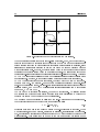
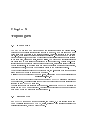
Phospholipase A2 ready to attack a lecithin
mono layer
i
GROMACS USER MANUAL
Version 2.0
November 5, 1999
David van der Spoel
Aldert R. van Buuren
Emile Apol
Pieter J. Meulenho
D. Peter Tieleman
Alfons L.T.M. Sijbers
Berk Hess
K. Anton Feenstra
Erik Lindahl
Rudi van Drunen
Herman J.C. Berendsen
BIOSON
(c) Copyright.
BIOSON Research Institute and
Laboratory of Biophysical Chemistry
University of Groningen
Nijenborgh 4
9747 AG Groningen
The Netherlands
Fax: +31 (0)50 63 4800
ii
Preface & Disclaimer.
This manual is not complete and has no pretention to be complete, due to lack of time of
the contributors. It is meant as a source of information and references for the GROMACS
user. It contains the background physics of MD simulations and is still being worked on
which in some cases means that the information is not correct.
When citing this document in any scientic publication please refer to it as:
van der Spoel, D., A. R. van Buuren, E. Apol, P. J. Meulenho, D. P.
Tieleman, A. L. T. M. Sijbers, B. Hess, K. A. Feenstra, E. Lindahl, R. van
Drunen and H. J. C. Berendsen Gromacs User Manual version 2.0
Nijenborgh 4, 9747 AG Groningen, The Netherlands. Internet:
http://md.chem.rug.nl/~gmx 1999
or, if you use BibTeX, you can directly copy the following:
@Manual{gmx20,
title =
author =
address =
year =
"Gromacs {U}ser {M}anual version 2.0",
"David van der Spoel and Aldert R. van Buuren and Emile
Apol and Pieter J. Meulenhoff and D. Peter Tieleman and
Alfons L. T. M. Sij\-bers and Berk Hess and K. Anton
Feenstra and Erik Lindahl and Rudi van Drunen
and Herman J. C. Berendsen",
"Nij\-enborgh 4, 9747 AG Groningen, The Netherlands.
Internet: http://md.chem.rug.nl/\~{ }gmx",
"1999"
}
Please do also cite the original GROMACS paper [1].
Any comment is welcome, please send it by e-mail to [email protected]
Groningen, November 5, 1999
BIOSON Research Institute and Department of Biophysical Chemistry
University of Groningen
Nijenborgh 4
9747 AG Groningen
The Netherlands
Fax: 31-50-634800
iii
Online Manual
If you have access to a WWW browser such as NCSA mosaic or Netscape please look up
our HTML page:
http://md.chem.rug.nl/~gmx.
Violated Copyrights
The following commercial thingies may be mentioned here and there in the text (plus some
that we forgot here).
GROMOS is a trademark of Biomos B.V.
SPARC
is a trademark of Sun Microsystems inc. and Texas Instruments inc.
CM5
is a trademark of Thinking Machines inc.
Quanta
is a trademark of Molecular Simulations inc.
Cerius
is a trademark of Molecular Simulations inc.
HyperChem is a trademark of AutoDesk inc.
The gure on front page was made with Molscript [2].
iv
Contents
1 Introduction.
1
2 Denitions and Units.
9
1.1 Computational Chemistry and Molecular Modeling . . . . . . . . . . . . . .
1.2 Molecular Dynamics Simulations . . . . . . . . . . . . . . . . . . . . . . . .
1.3 Energy Minimization and Search Methods . . . . . . . . . . . . . . . . . . .
1
2
5
2.1 Notation . . . . . . . . . . . . . . . . . . . . . . . . . . . . . . . . . . . . . . 9
2.2 MD units . . . . . . . . . . . . . . . . . . . . . . . . . . . . . . . . . . . . . 9
2.3 Reduced units . . . . . . . . . . . . . . . . . . . . . . . . . . . . . . . . . . . 11
3 Algorithms
3.1
3.2
3.3
3.4
3.5
3.6
3.7
3.8
Introduction . . . . . . . . . .
Periodic boundary conditions
The group concept . . . . . .
Molecular Dynamics . . . . .
3.4.1 Initial conditions . . .
3.4.2 Compute forces . . . .
3.4.3 Update conguration .
3.4.4 Constraint algorithms
3.4.5 Output step . . . . . .
Simulated Annealing . . . . .
Langevin Dynamics . . . . . .
Energy Minimization . . . . .
3.7.1 Steepest Descent . . .
3.7.2 Conjugate Gradient .
Normal Mode Analysis . . . .
.
.
.
.
.
.
.
.
.
.
.
.
.
.
.
.
.
.
.
.
.
.
.
.
.
.
.
.
.
.
.
.
.
.
.
.
.
.
.
.
.
.
.
.
.
.
.
.
.
.
.
.
.
.
.
.
.
.
.
.
.
.
.
.
.
.
.
.
.
.
.
.
.
.
.
.
.
.
.
.
.
.
.
.
.
.
.
.
.
.
.
.
.
.
.
.
.
.
.
.
.
.
.
.
.
.
.
.
.
.
.
.
.
.
.
.
.
.
.
.
.
.
.
.
.
.
.
.
.
.
.
.
.
.
.
.
.
.
.
.
.
.
.
.
.
.
.
.
.
.
.
.
.
.
.
.
.
.
.
.
.
.
.
.
.
.
.
.
.
.
.
.
.
.
.
.
.
.
.
.
.
.
.
.
.
.
.
.
.
.
.
.
.
.
.
.
.
.
.
.
.
.
.
.
.
.
.
.
.
.
.
.
.
.
.
.
.
.
.
.
.
.
.
.
.
.
.
.
.
.
.
.
.
.
.
.
.
.
.
.
.
.
.
.
.
.
.
.
.
.
.
.
.
.
.
.
.
.
.
.
.
.
.
.
.
.
.
.
.
.
.
.
.
.
.
.
.
.
.
.
.
.
.
.
.
.
.
.
.
.
.
.
.
.
.
.
.
.
.
.
.
.
.
.
.
.
.
.
.
.
.
.
.
.
.
.
.
.
.
.
.
.
.
.
.
.
.
.
.
.
.
.
.
.
.
.
.
.
.
.
.
.
.
.
.
.
.
.
.
.
.
.
.
.
.
.
.
.
.
.
.
.
.
.
.
.
.
.
.
.
.
.
.
.
.
.
.
.
.
.
.
.
.
.
.
.
.
.
.
.
13
13
13
15
15
17
18
21
24
28
29
29
29
30
30
30
vi
CONTENTS
3.9 Free energy perturbation . . . . . . . . . . . . . . . .
3.10 Essential Dynamics Sampling . . . . . . . . . . . . .
3.11 Parallelization . . . . . . . . . . . . . . . . . . . . . .
3.11.1 Methods of parallelization . . . . . . . . . . .
3.11.2 MD on a ring of processors . . . . . . . . . .
3.12 Parallel Molecular Dynamics . . . . . . . . . . . . .
3.12.1 Domain decomposition . . . . . . . . . . . . .
3.12.2 Domain decomposition for non-bonded forces
3.12.3 Parallel PPPM . . . . . . . . . . . . . . . . .
3.12.4 Parallel sorting . . . . . . . . . . . . . . . . .
4 Force elds
.
.
.
.
.
.
.
.
.
.
.
.
.
.
.
.
.
.
.
.
.
.
.
.
.
.
.
.
.
.
.
.
.
.
.
.
.
.
.
.
.
.
.
.
.
.
.
.
.
.
.
.
.
.
.
.
.
.
.
.
.
.
.
.
.
.
.
.
.
.
4.1 Non-bonded interactions . . . . . . . . . . . . . . . . . . . . . . .
4.1.1 The Lennard-Jones interaction . . . . . . . . . . . . . . .
4.1.2 Buckingham potential . . . . . . . . . . . . . . . . . . . .
4.1.3 Coulomb interaction . . . . . . . . . . . . . . . . . . . . .
4.1.4 Coulomb interaction with reaction eld . . . . . . . . . .
4.1.5 Modied non-bonded interactions . . . . . . . . . . . . . .
4.1.6 Modied short-range interactions with Ewald summation
4.2 Bonded interactions . . . . . . . . . . . . . . . . . . . . . . . . .
4.2.1 Bond stretching . . . . . . . . . . . . . . . . . . . . . . . .
4.2.2 Morse potential bond stretching . . . . . . . . . . . . . .
4.2.3 Bond angle vibration . . . . . . . . . . . . . . . . . . . . .
4.2.4 Improper dihedrals . . . . . . . . . . . . . . . . . . . . . .
4.2.5 Proper dihedrals . . . . . . . . . . . . . . . . . . . . . . .
4.2.6 Special interactions . . . . . . . . . . . . . . . . . . . . . .
4.2.7 Position restraints . . . . . . . . . . . . . . . . . . . . . .
4.2.8 Angle restraints . . . . . . . . . . . . . . . . . . . . . . . .
4.2.9 Distance restraints . . . . . . . . . . . . . . . . . . . . . .
4.3 Free energy calculations . . . . . . . . . . . . . . . . . . . . . . .
4.3.1 Near linear thermodynamic integration . . . . . . . . . .
4.4 Methods . . . . . . . . . . . . . . . . . . . . . . . . . . . . . . . .
4.4.1 Exclusions and 1-4 Interactions. . . . . . . . . . . . . . .
4.4.2 Charge Groups. . . . . . . . . . . . . . . . . . . . . . . . .
.
.
.
.
.
.
.
.
.
.
.
.
.
.
.
.
.
.
.
.
.
.
.
.
.
.
.
.
.
.
.
.
.
.
.
.
.
.
.
.
.
.
.
.
.
.
.
.
.
.
.
.
.
.
.
.
.
.
.
.
.
.
.
.
.
.
.
.
.
.
.
.
.
.
.
.
.
.
.
.
.
.
.
.
.
.
.
.
.
.
.
.
.
.
.
.
.
.
.
.
.
.
.
.
.
.
.
.
.
.
.
.
.
.
.
.
.
.
.
.
.
.
.
.
.
.
.
.
.
.
.
.
.
.
.
.
.
.
.
.
.
.
.
.
.
.
.
.
.
.
.
.
.
.
.
.
.
.
.
.
.
.
.
.
.
.
.
.
.
.
.
.
.
.
.
.
.
.
.
.
.
.
.
.
.
.
.
.
.
.
.
.
31
31
32
32
34
37
38
38
40
41
43
44
44
45
46
46
47
49
50
50
51
52
53
54
56
56
57
57
61
63
65
65
65
CONTENTS
4.5
4.6
4.7
4.8
4.4.3 Treatment of cut-os . . . . . .
Dummy atoms. . . . . . . . . . . . . .
Long Range Electrostatics . . . . . . .
4.6.1 Ewald summation . . . . . . .
4.6.2 PME . . . . . . . . . . . . . . .
4.6.3 PPPM . . . . . . . . . . . . . .
4.6.4 Optimizing Fourier transforms
All-hydrogen forceeld . . . . . . . . .
GROMOS-96 notes . . . . . . . . . . .
4.8.1 The GROMOS-96 force eld .
4.8.2 GROMOS-96 les . . . . . . .
5 Topologies
5.1 Introduction . . . . . . . . . . . . . . .
5.2 Particle type . . . . . . . . . . . . . .
5.2.1 Atom types . . . . . . . . . . .
5.2.2 Dummy atoms . . . . . . . . .
5.3 Parameter les . . . . . . . . . . . . .
5.3.1 Atoms . . . . . . . . . . . . . .
5.3.2 Bonded parameters . . . . . . .
5.3.3 Non-bonded parameters . . . .
5.3.4 Exclusions and 1-4 interaction
5.3.5 Residue database . . . . . . . .
5.3.6 Hydrogen database . . . . . . .
5.3.7 Termini database . . . . . . . .
5.4 File formats . . . . . . . . . . . . . . .
5.4.1 Topology le . . . . . . . . . .
5.4.2 Molecule.itp le . . . . . . . . .
5.4.3 Ifdef option . . . . . . . . . . .
5.4.4 Coordinate le . . . . . . . . .
6 Special Topics
vii
.
.
.
.
.
.
.
.
.
.
.
.
.
.
.
.
.
.
.
.
.
.
.
.
.
.
.
.
.
.
.
.
.
.
.
.
.
.
.
.
.
.
.
.
.
.
.
.
.
.
.
.
.
.
.
.
.
.
.
.
.
.
.
.
.
.
.
.
.
.
.
.
.
.
.
.
.
.
.
.
.
.
.
.
.
.
.
.
.
.
.
.
.
.
.
.
.
.
.
.
.
.
.
.
.
.
.
.
.
.
.
.
.
.
.
.
.
.
.
.
.
.
.
.
.
.
.
.
.
.
.
.
.
.
.
.
.
.
.
.
.
.
.
.
.
.
.
.
.
.
.
.
.
.
.
.
.
.
.
.
.
.
.
.
.
.
.
.
.
.
.
.
.
.
.
.
.
.
.
.
.
.
.
.
.
.
.
.
.
.
.
.
.
.
.
.
.
.
.
.
.
.
.
.
.
.
.
.
.
.
.
.
.
.
.
.
.
.
.
.
.
.
.
.
.
.
.
.
.
.
.
.
.
.
.
.
.
.
.
.
.
.
.
.
.
.
.
.
.
.
.
.
.
.
.
.
.
.
.
.
.
.
.
.
.
.
.
.
.
.
.
.
.
.
.
.
.
.
.
.
.
.
.
.
.
.
.
.
.
.
.
.
.
.
.
.
.
.
.
.
.
.
.
.
.
.
.
.
.
.
.
.
.
.
.
.
.
.
.
.
.
.
.
.
.
.
.
.
.
.
.
.
.
.
.
.
.
.
.
.
.
.
.
.
.
.
.
.
.
.
.
.
.
.
.
.
.
.
.
.
.
.
.
.
.
.
.
.
.
.
.
.
.
.
.
.
.
.
.
.
.
.
.
.
.
.
.
.
.
.
.
.
.
.
.
.
.
.
.
.
.
.
.
.
.
.
.
.
.
.
.
.
.
.
.
.
.
.
.
.
.
.
.
.
.
.
.
.
.
.
.
.
.
.
.
.
.
.
.
.
.
.
.
.
.
.
.
.
.
.
.
.
.
.
.
.
.
.
.
.
.
.
.
.
.
.
.
.
.
.
.
.
.
.
.
.
.
.
.
.
.
.
.
.
.
.
.
.
.
.
.
.
.
.
.
.
.
.
.
.
.
.
.
.
.
.
.
.
.
.
.
.
.
.
.
.
.
.
.
.
.
.
.
.
.
.
.
.
.
.
.
.
.
.
.
.
.
.
.
.
.
.
.
.
.
.
.
.
.
.
.
.
.
.
.
.
.
.
.
.
.
.
.
.
.
.
.
.
.
.
.
.
.
.
.
.
.
.
.
.
.
.
.
.
.
.
.
.
66
67
69
69
70
71
72
73
73
73
73
75
75
75
76
77
78
78
79
80
81
81
83
84
86
86
92
93
94
97
6.1 Calculating potentials of mean force: the pull code . . . . . . . . . . . . . . 97
6.1.1 Overview . . . . . . . . . . . . . . . . . . . . . . . . . . . . . . . . . 97
6.1.2 Usage . . . . . . . . . . . . . . . . . . . . . . . . . . . . . . . . . . . 98
viii
CONTENTS
6.1.3 Output . . . . . . . . . . . . . . . . . . . .
6.1.4 Limitations . . . . . . . . . . . . . . . . . .
6.1.5 Implementation . . . . . . . . . . . . . . . .
6.1.6 Future development . . . . . . . . . . . . .
6.2 Removing fastest degrees of freedom . . . . . . . .
6.2.1 Hydrogen bond-angle vibrations . . . . . .
6.2.2 Out-of-plane vibrations in aromatic groups
6.3 Running with PVM. . . . . . . . . . . . . . . . . .
6.4 Running with MPI . . . . . . . . . . . . . . . . . .
7 Run parameters and Programs
7.1 Online and html manuals . . . .
7.2 File types . . . . . . . . . . . . .
7.3 Run Parameters . . . . . . . . .
7.3.1 General . . . . . . . . . .
7.3.2 Preprocessing . . . . . . .
7.3.3 Run control . . . . . . . .
7.3.4 Langevin dynamics . . . .
7.3.5 Energy minimization . . .
7.3.6 Output control . . . . . .
7.3.7 Neighbor searching . . . .
7.3.8 Electrostatics and VdW .
7.3.9 Temperature coupling . .
7.3.10 Pressure coupling . . . . .
7.3.11 Simulated annealing . . .
7.3.12 Velocity generation . . . .
7.3.13 Solvent optimization . . .
7.3.14 Bonds . . . . . . . . . . .
7.3.15 NMR renement . . . . .
7.3.16 Free Energy Perturbation
7.3.17 Non-equilibrium MD . . .
7.3.18 Electric elds . . . . . . .
7.3.19 User dened thingies . . .
7.4 Program Options . . . . . . . . .
.
.
.
.
.
.
.
.
.
.
.
.
.
.
.
.
.
.
.
.
.
.
.
.
.
.
.
.
.
.
.
.
.
.
.
.
.
.
.
.
.
.
.
.
.
.
.
.
.
.
.
.
.
.
.
.
.
.
.
.
.
.
.
.
.
.
.
.
.
.
.
.
.
.
.
.
.
.
.
.
.
.
.
.
.
.
.
.
.
.
.
.
.
.
.
.
.
.
.
.
.
.
.
.
.
.
.
.
.
.
.
.
.
.
.
.
.
.
.
.
.
.
.
.
.
.
.
.
.
.
.
.
.
.
.
.
.
.
.
.
.
.
.
.
.
.
.
.
.
.
.
.
.
.
.
.
.
.
.
.
.
.
.
.
.
.
.
.
.
.
.
.
.
.
.
.
.
.
.
.
.
.
.
.
.
.
.
.
.
.
.
.
.
.
.
.
.
.
.
.
.
.
.
.
.
.
.
.
.
.
.
.
.
.
.
.
.
.
.
.
.
.
.
.
.
.
.
.
.
.
.
.
.
.
.
.
.
.
.
.
.
.
.
.
.
.
.
.
.
.
.
.
.
.
.
.
.
.
.
.
.
.
.
.
.
.
.
.
.
.
.
.
.
.
.
.
.
.
.
.
.
.
.
.
.
.
.
.
.
.
.
.
.
.
.
.
.
.
.
.
.
.
.
.
.
.
.
.
.
.
.
.
.
.
.
.
.
.
.
.
.
.
.
.
.
.
.
.
.
.
.
.
.
.
.
.
.
.
.
.
.
.
.
.
.
.
.
.
.
.
.
.
.
.
.
.
.
.
.
.
.
.
.
.
.
.
.
.
.
.
.
.
.
.
.
.
.
.
.
.
.
.
.
.
.
.
.
.
.
.
.
.
.
.
.
.
.
.
.
.
.
.
.
.
.
.
.
.
.
.
.
.
.
.
.
.
.
.
.
.
.
.
.
.
.
.
.
.
.
.
.
.
.
.
.
.
.
.
.
.
.
.
.
.
.
.
.
.
.
.
.
.
.
.
.
.
.
.
.
.
.
.
.
.
.
.
.
.
.
.
.
.
.
.
.
.
.
.
.
.
.
.
.
.
.
.
.
.
.
.
.
.
.
.
.
.
.
.
.
.
.
.
.
.
.
.
.
.
.
.
.
.
.
.
.
.
.
.
.
.
.
.
.
.
.
.
.
.
.
.
.
.
.
.
.
.
.
.
.
.
.
.
.
.
.
.
.
.
.
.
.
.
.
.
.
.
.
.
.
.
.
.
.
.
.
.
.
.
.
.
.
.
.
.
.
.
.
.
.
.
.
.
.
.
.
.
.
.
.
.
.
.
.
.
.
.
.
.
.
.
.
.
.
.
.
.
.
.
.
.
.
.
.
.
.
.
.
.
.
.
.
.
.
.
.
.
.
.
.
.
.
.
.
.
.
.
.
.
.
.
.
.
.
.
.
.
. 101
. 102
. 102
. 102
. 102
. 103
. 105
. 106
. 107
109
. 109
. 109
. 109
. 109
. 111
. 111
. 112
. 112
. 112
. 113
. 114
. 116
. 117
. 118
. 118
. 118
. 119
. 120
. 121
. 121
. 122
. 122
. 122
CONTENTS
ix
7.5 Programs by topic . . . . . . . . . . . . . . . . . . . . . . . . . . . . . . . . 123
8 Analysis.
8.1
8.2
8.3
8.4
8.5
8.6
8.7
8.8
8.9
8.10
8.11
8.12
8.13
Groups in Analysis. . . . . . . . . . . . . . . . .
Looking at your trajectory . . . . . . . . . . . .
General properties . . . . . . . . . . . . . . . .
Radial distribution functions . . . . . . . . . .
Correlation functions . . . . . . . . . . . . . . .
8.5.1 Theory of correlation functions . . . . .
8.5.2 Using FFT for computation of the ACF
8.5.3 Special forms of the ACF . . . . . . . .
8.5.4 Some Applications . . . . . . . . . . . .
8.5.5 Mean Square Displacement . . . . . . .
Bonds, angles and dihedrals . . . . . . . . . . .
Radius of gyration and distances . . . . . . . .
Root mean square deviations in structure . . .
Covariance analysis . . . . . . . . . . . . . . . .
Hydrogen bonds . . . . . . . . . . . . . . . . .
Protein related items . . . . . . . . . . . . . . .
Interface related items . . . . . . . . . . . . . .
Chemical shifts . . . . . . . . . . . . . . . . . .
A Technical Details.
A.1 Installation. . . . . . . . . . . .
A.2 Single or Double precision . . .
A.3 Porting GROMACS . . . . . . .
A.3.1 Multi-processor Porting
A.4 Environment Variables . . . . .
B Some implementation details.
.
.
.
.
.
.
.
.
.
.
.
.
.
.
.
.
.
.
.
.
.
.
.
.
.
.
.
.
.
.
.
.
.
.
.
B.1 Single Sum Virial in GROMACS . . . . . . .
B.1.1 Virial. . . . . . . . . . . . . . . . . .
B.1.2 Virial from non-bonded forces. . . .
B.1.3 The intramolecular shift (mol-shift).
B.1.4 Virial from Covalent Bonds. . . . . .
.
.
.
.
.
.
.
.
.
.
.
.
.
.
.
.
.
.
.
.
.
.
.
.
.
.
.
.
.
.
.
.
.
.
.
.
.
.
.
.
.
.
.
.
.
.
.
.
.
.
.
.
.
.
.
.
.
.
.
.
.
.
.
.
.
.
.
.
.
.
.
.
.
.
.
.
.
.
.
.
.
.
.
.
.
.
.
.
.
.
.
.
.
.
.
.
.
.
.
.
.
.
.
.
.
.
.
.
.
.
.
.
.
.
.
.
.
.
.
.
.
.
.
.
.
.
.
.
.
.
.
.
.
.
.
.
.
.
.
.
.
.
.
.
.
.
.
.
.
.
.
.
.
.
.
.
.
.
.
.
.
.
.
.
.
.
.
.
.
.
.
.
.
.
.
.
.
.
.
.
.
.
.
.
.
.
.
.
.
.
.
.
.
.
.
.
.
.
.
.
.
.
.
.
.
.
.
.
.
.
.
.
.
.
.
.
.
.
.
.
.
.
.
.
.
.
.
.
.
.
.
.
.
.
.
.
.
.
.
.
.
.
.
.
.
.
.
.
.
.
.
.
.
.
.
.
.
.
.
.
.
.
.
.
.
.
.
.
.
.
.
.
.
.
.
.
.
.
.
.
.
.
.
.
.
.
.
.
.
.
.
.
.
.
.
.
.
.
.
.
.
.
.
.
.
.
.
.
.
.
.
.
.
.
.
.
.
.
.
.
.
.
.
.
.
.
.
.
.
.
.
.
.
.
.
.
.
.
.
.
.
.
.
.
.
.
.
.
.
.
.
.
.
.
.
.
.
.
.
.
.
.
.
.
.
.
.
.
.
.
.
.
.
.
.
.
.
.
.
.
.
.
.
.
.
.
.
.
.
.
.
.
.
.
.
.
.
.
.
.
.
.
.
.
.
.
.
.
.
.
.
.
.
.
.
.
.
.
.
.
.
.
.
.
.
.
.
.
.
.
.
.
.
.
.
.
.
.
.
.
127
. 127
. 128
. 129
. 129
. 131
. 131
. 132
. 132
. 132
. 133
. 133
. 136
. 137
. 138
. 139
. 141
. 143
. 144
145
. 145
. 145
. 146
. 146
. 147
149
. 149
. 149
. 150
. 150
. 151
x
CONTENTS
B.1.5 Virial from Shake. . . . . . . . . . . . . . . .
B.2 Optimizations . . . . . . . . . . . . . . . . . . . . . .
B.2.1 Inner Loop for Water . . . . . . . . . . . . .
B.2.2 Shake for Water - SETTLE . . . . . . . . . .
B.2.3 Fortran Code . . . . . . . . . . . . . . . . . .
B.3 Computation of the 1.0/sqrt function. . . . . . . . .
B.3.1 Introduction. . . . . . . . . . . . . . . . . . .
B.3.2 General . . . . . . . . . . . . . . . . . . . . .
B.3.3 Applied to oating point numbers . . . . . .
B.3.4 Specication of the lookup table . . . . . . .
B.3.5 Separate exponent and fraction computation
B.3.6 Implementation . . . . . . . . . . . . . . . . .
B.4 Tabulated functions . . . . . . . . . . . . . . . . . .
B.4.1 Your own potential function . . . . . . . . . .
.
.
.
.
.
.
.
.
.
.
.
.
.
.
.
.
.
.
.
.
.
.
.
.
.
.
.
.
.
.
.
.
.
.
.
.
.
.
.
.
.
.
.
.
.
.
.
.
.
.
.
.
.
.
.
.
.
.
.
.
.
.
.
.
.
.
.
.
.
.
.
.
.
.
.
.
.
.
.
.
.
.
.
.
.
.
.
.
.
.
.
.
.
.
.
.
.
.
.
.
.
.
.
.
.
.
.
.
.
.
.
.
.
.
.
.
.
.
.
.
.
.
.
.
.
.
.
.
.
.
.
.
.
.
.
.
.
.
.
.
.
.
.
.
.
.
.
.
.
.
.
.
.
.
.
.
.
.
.
.
.
.
.
.
.
.
.
.
. 152
. 152
. 152
. 153
. 153
. 154
. 154
. 154
. 155
. 156
. 157
. 158
. 159
. 160
C Long range corrections
161
D Averages and uctuations
165
C.1 Dispersion . . . . . . . . . . . . . . . . . . . . . . . . . . . . . . . . . . . . . 161
C.1.1 Energy . . . . . . . . . . . . . . . . . . . . . . . . . . . . . . . . . . . 161
C.1.2 Virial and pressure . . . . . . . . . . . . . . . . . . . . . . . . . . . . 162
D.1 Formulae for averaging . . . . . . .
D.2 Implementation . . . . . . . . . . .
D.2.1 Part of a Simulation . . . .
D.2.2 Combining two simulations
D.2.3 Summing energy terms . . .
E Manual Pages
E.1
E.2
E.3
E.4
E.5
E.6
E.7
do dssp .
editconf .
eneconv .
g anaeig .
g analyze
g angle . .
g bond . .
.
.
.
.
.
.
.
.
.
.
.
.
.
.
.
.
.
.
.
.
.
.
.
.
.
.
.
.
.
.
.
.
.
.
.
.
.
.
.
.
.
.
.
.
.
.
.
.
.
.
.
.
.
.
.
.
.
.
.
.
.
.
.
.
.
.
.
.
.
.
.
.
.
.
.
.
.
.
.
.
.
.
.
.
.
.
.
.
.
.
.
.
.
.
.
.
.
.
.
.
.
.
.
.
.
.
.
.
.
.
.
.
.
.
.
.
.
.
.
.
.
.
.
.
.
.
.
.
.
.
.
.
.
.
.
.
.
.
.
.
.
.
.
.
.
.
.
.
.
.
.
.
.
.
.
.
.
.
.
.
.
.
.
.
.
.
.
.
.
.
.
.
.
.
.
.
.
.
.
.
.
.
.
.
.
.
.
.
.
.
.
.
.
.
.
.
.
.
.
.
.
.
.
.
.
.
.
.
.
.
.
.
.
.
.
.
.
.
.
.
.
.
.
.
.
.
.
.
.
.
.
.
.
.
.
.
.
.
.
.
.
.
.
.
.
.
.
.
.
.
.
.
.
.
.
.
.
.
.
.
.
.
.
.
.
.
.
.
.
.
.
.
.
.
.
.
.
.
.
.
.
.
.
.
.
.
.
.
.
.
.
.
.
.
.
.
.
.
.
.
.
.
.
.
.
.
.
.
.
.
.
.
.
.
.
.
.
.
.
.
.
.
.
.
.
.
.
.
.
.
.
.
.
.
.
.
.
.
.
.
.
.
.
.
.
.
.
.
.
.
.
.
.
.
.
.
.
.
.
.
.
.
. 165
. 166
. 166
. 167
. 168
171
. 171
. 172
. 173
. 173
. 174
. 175
. 176
CONTENTS
E.8 g chi . . . .
E.9 g cluster . .
E.10 g com . . .
E.11 g confrms .
E.12 g covar . . .
E.13 g density . .
E.14 g dielectric
E.15 g dih . . . .
E.16 g dipoles . .
E.17 g disre . . .
E.18 g dist . . .
E.19 g enemat .
E.20 g energy . .
E.21 g gyrate . .
E.22 g h2order .
E.23 g hbond . .
E.24 g helix . . .
E.25 g mdmat . .
E.26 g mindist .
E.27 g msd . . .
E.28 g nmeig . .
E.29 g nmens . .
E.30 g order . . .
E.31 g potential .
E.32 g rama . . .
E.33 g rdens . .
E.34 g rdf . . . .
E.35 g rms . . .
E.36 g rmsdist .
E.37 g rmsf . . .
E.38 g rotacf . .
E.39 g saltbr . .
E.40 g sas . . . .
E.41 g sgangle .
xi
.
.
.
.
.
.
.
.
.
.
.
.
.
.
.
.
.
.
.
.
.
.
.
.
.
.
.
.
.
.
.
.
.
.
.
.
.
.
.
.
.
.
.
.
.
.
.
.
.
.
.
.
.
.
.
.
.
.
.
.
.
.
.
.
.
.
.
.
.
.
.
.
.
.
.
.
.
.
.
.
.
.
.
.
.
.
.
.
.
.
.
.
.
.
.
.
.
.
.
.
.
.
.
.
.
.
.
.
.
.
.
.
.
.
.
.
.
.
.
.
.
.
.
.
.
.
.
.
.
.
.
.
.
.
.
.
.
.
.
.
.
.
.
.
.
.
.
.
.
.
.
.
.
.
.
.
.
.
.
.
.
.
.
.
.
.
.
.
.
.
.
.
.
.
.
.
.
.
.
.
.
.
.
.
.
.
.
.
.
.
.
.
.
.
.
.
.
.
.
.
.
.
.
.
.
.
.
.
.
.
.
.
.
.
.
.
.
.
.
.
.
.
.
.
.
.
.
.
.
.
.
.
.
.
.
.
.
.
.
.
.
.
.
.
.
.
.
.
.
.
.
.
.
.
.
.
.
.
.
.
.
.
.
.
.
.
.
.
.
.
.
.
.
.
.
.
.
.
.
.
.
.
.
.
.
.
.
.
.
.
.
.
.
.
.
.
.
.
.
.
.
.
.
.
.
.
.
.
.
.
.
.
.
.
.
.
.
.
.
.
.
.
.
.
.
.
.
.
.
.
.
.
.
.
.
.
.
.
.
.
.
.
.
.
.
.
.
.
.
.
.
.
.
.
.
.
.
.
.
.
.
.
.
.
.
.
.
.
.
.
.
.
.
.
.
.
.
.
.
.
.
.
.
.
.
.
.
.
.
.
.
.
.
.
.
.
.
.
.
.
.
.
.
.
.
.
.
.
.
.
.
.
.
.
.
.
.
.
.
.
.
.
.
.
.
.
.
.
.
.
.
.
.
.
.
.
.
.
.
.
.
.
.
.
.
.
.
.
.
.
.
.
.
.
.
.
.
.
.
.
.
.
.
.
.
.
.
.
.
.
.
.
.
.
.
.
.
.
.
.
.
.
.
.
.
.
.
.
.
.
.
.
.
.
.
.
.
.
.
.
.
.
.
.
.
.
.
.
.
.
.
.
.
.
.
.
.
.
.
.
.
.
.
.
.
.
.
.
.
.
.
.
.
.
.
.
.
.
.
.
.
.
.
.
.
.
.
.
.
.
.
.
.
.
.
.
.
.
.
.
.
.
.
.
.
.
.
.
.
.
.
.
.
.
.
.
.
.
.
.
.
.
.
.
.
.
.
.
.
.
.
.
.
.
.
.
.
.
.
.
.
.
.
.
.
.
.
.
.
.
.
.
.
.
.
.
.
.
.
.
.
.
.
.
.
.
.
.
.
.
.
.
.
.
.
.
.
.
.
.
.
.
.
.
.
.
.
.
.
.
.
.
.
.
.
.
.
.
.
.
.
.
.
.
.
.
.
.
.
.
.
.
.
.
.
.
.
.
.
.
.
.
.
.
.
.
.
.
.
.
.
.
.
.
.
.
.
.
.
.
.
.
.
.
.
.
.
.
.
.
.
.
.
.
.
.
.
.
.
.
.
.
.
.
.
.
.
.
.
.
.
.
.
.
.
.
.
.
.
.
.
.
.
.
.
.
.
.
.
.
.
.
.
.
.
.
.
.
.
.
.
.
.
.
.
.
.
.
.
.
.
.
.
.
.
.
.
.
.
.
.
.
.
.
.
.
.
.
.
.
.
.
.
.
.
.
.
.
.
.
.
.
.
.
.
.
.
.
.
.
.
.
.
.
.
.
.
.
.
.
.
.
.
.
.
.
.
.
.
.
.
.
.
.
.
.
.
.
.
.
.
.
.
.
.
.
.
.
.
.
.
.
.
.
.
.
.
.
.
.
.
.
.
.
.
.
.
.
.
.
.
.
.
.
.
.
.
.
.
.
.
.
.
.
.
.
.
.
.
.
.
.
.
.
.
.
.
.
.
.
.
.
.
.
.
.
.
.
.
.
.
.
.
.
.
.
.
.
.
.
.
.
.
.
.
.
.
.
.
.
.
.
.
.
.
.
.
.
.
.
.
.
.
.
.
.
.
.
.
.
.
.
.
.
.
.
.
.
.
.
.
.
.
.
.
.
.
.
.
.
.
.
.
.
.
.
.
.
.
.
.
.
.
.
.
.
.
.
.
.
.
.
.
.
.
.
.
.
.
.
.
.
.
.
.
.
.
.
.
.
.
.
.
.
.
.
.
.
.
.
.
.
.
.
.
.
.
.
.
.
.
.
.
.
.
.
.
.
.
.
.
.
.
.
.
.
.
.
.
.
.
.
.
.
.
.
.
.
.
.
.
.
.
.
.
.
.
.
.
.
.
.
.
.
.
.
.
.
.
.
.
.
.
.
.
.
.
.
.
.
.
.
.
.
.
.
.
.
.
.
.
.
.
.
.
.
.
.
.
.
.
.
.
.
.
.
.
.
.
.
.
.
.
.
.
.
.
.
.
.
.
.
.
.
.
.
.
.
.
.
.
.
.
.
.
.
.
.
.
.
.
.
.
.
.
.
.
.
.
.
.
.
.
.
.
.
.
.
.
.
.
.
.
.
.
.
.
.
.
.
.
.
.
.
.
.
.
.
.
.
. 177
. 178
. 179
. 179
. 180
. 180
. 181
. 182
. 182
. 184
. 184
. 185
. 185
. 186
. 187
. 187
. 189
. 190
. 190
. 191
. 191
. 192
. 192
. 193
. 193
. 194
. 194
. 195
. 196
. 196
. 197
. 198
. 198
. 199
xii
CONTENTS
E.42 g velacc . .
E.43 genbox . . .
E.44 genconf . .
E.45 gendr . . .
E.46 genion . . .
E.47 genpr . . .
E.48 gmxcheck .
E.49 gmxdump .
E.50 grompp . .
E.51 highway . .
E.52 make ndx .
E.53 mdrun . . .
E.54 mk angndx
E.55 ngmx . . . .
E.56 nmrun . . .
E.57 pdb2gmx .
E.58 protonate .
E.59 tpbconv . .
E.60 trjcat . . . .
E.61 trjconv . . .
E.62 wheel . . .
E.63 xpm2ps . .
E.64 xrama . . .
.
.
.
.
.
.
.
.
.
.
.
.
.
.
.
.
.
.
.
.
.
.
.
.
.
.
.
.
.
.
.
.
.
.
.
.
.
.
.
.
.
.
.
.
.
.
.
.
.
.
.
.
.
.
.
.
.
.
.
.
.
.
.
.
.
.
.
.
.
.
.
.
.
.
.
.
.
.
.
.
.
.
.
.
.
.
.
.
.
.
.
.
.
.
.
.
.
.
.
.
.
.
.
.
.
.
.
.
.
.
.
.
.
.
.
.
.
.
.
.
.
.
.
.
.
.
.
.
.
.
.
.
.
.
.
.
.
.
.
.
.
.
.
.
.
.
.
.
.
.
.
.
.
.
.
.
.
.
.
.
.
.
.
.
.
.
.
.
.
.
.
.
.
.
.
.
.
.
.
.
.
.
.
.
.
.
.
.
.
.
.
.
.
.
.
.
.
.
.
.
.
.
.
.
.
.
.
.
.
.
.
.
.
.
.
.
.
.
.
.
.
.
.
.
.
.
.
.
.
.
.
.
.
.
.
.
.
.
.
.
.
.
.
.
.
.
.
.
.
.
.
.
.
.
.
.
.
.
.
.
.
.
.
.
.
.
.
.
.
.
.
.
.
.
.
.
.
.
.
.
.
.
.
.
.
.
.
.
.
.
.
.
.
.
.
.
.
.
.
.
.
.
.
.
.
.
.
.
.
.
.
.
.
.
.
.
.
.
.
.
.
.
.
.
.
.
.
.
.
.
.
.
.
.
.
.
.
.
.
.
.
.
.
.
.
.
.
.
.
.
.
.
.
.
.
.
.
.
.
.
.
.
.
.
.
.
.
.
.
.
.
.
.
.
.
.
.
.
.
.
.
.
.
.
.
.
.
.
.
.
.
.
.
.
.
.
.
.
.
.
.
.
.
.
.
.
.
.
.
.
.
.
.
.
.
.
.
.
.
.
.
.
.
.
.
.
.
.
.
.
.
.
.
.
.
.
.
.
.
.
.
.
.
.
.
.
.
.
.
.
.
.
.
.
.
.
.
.
.
.
.
.
.
.
.
.
.
.
.
.
.
.
.
.
.
.
.
.
.
.
.
.
.
.
.
.
.
.
.
.
.
.
.
.
.
.
.
.
.
.
.
.
.
.
.
.
.
.
.
.
.
.
.
.
.
.
.
.
.
.
.
.
.
.
.
.
.
.
.
.
.
.
.
.
.
.
.
.
.
.
.
.
.
.
.
.
.
.
.
.
.
.
.
.
.
.
.
.
.
.
.
.
.
.
.
.
.
.
.
.
.
.
.
.
.
.
.
.
.
.
.
.
.
.
.
.
.
.
.
.
.
.
.
.
.
.
.
.
.
.
.
.
.
.
.
.
.
.
.
.
.
.
.
.
.
.
.
.
.
.
.
.
.
.
.
.
.
.
.
.
.
.
.
.
.
.
.
.
.
.
.
.
.
.
.
.
.
.
.
.
.
.
.
.
.
.
.
.
.
.
.
.
.
.
.
.
.
.
.
.
.
.
.
.
.
.
.
.
.
.
.
.
.
.
.
.
.
.
.
.
.
.
.
.
.
.
.
.
.
.
.
.
.
.
.
.
.
.
.
.
.
.
.
.
.
.
.
.
.
.
.
.
.
.
.
.
.
.
.
.
.
.
.
.
.
.
.
.
.
.
.
.
.
.
.
.
.
.
.
.
.
.
.
.
.
.
.
.
.
.
.
.
.
.
.
.
.
.
.
.
.
.
.
.
.
.
.
.
.
.
.
.
.
.
.
.
.
.
.
.
.
.
.
.
.
.
.
.
.
.
.
.
.
.
.
. 199
. 200
. 201
. 201
. 202
. 202
. 203
. 203
. 204
. 205
. 205
. 206
. 207
. 207
. 208
. 208
. 209
. 210
. 210
. 211
. 212
. 213
. 213
Bibliography
215
Index
221
List of Figures
3.1
3.2
3.3
3.4
3.5
3.6
3.7
3.8
3.9
3.10
3.11
3.12
3.13
Periodic boundary conditions in two dimensions. . . . . . . .
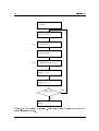
The global MD algorithm . . . . . . . . . . . . . . . . . . . .
A Maxwellian distribution, generated from random numbers.
The computational box in two dimensions. . . . . . . . . . . .
The Leap-Frog integration method. . . . . . . . . . . . . . . .
The MD update algorithm . . . . . . . . . . . . . . . . . . . .
The three position updates needed for one time step. . . . . .
Free energy cycles. . . . . . . . . . . . . . . . . . . . . . . . .
The interaction matrix. . . . . . . . . . . . . . . . . . . . . .
Interaction matrices for dierent N . . . . . . . . . . . . . . .
The Parallel MD algorithm. . . . . . . . . . . . . . . . . . . .
Data ow in a ring of processors. . . . . . . . . . . . . . . . .
Index in the coordinate array. . . . . . . . . . . . . . . . . . .
.
.
.
.
.
.
.
.
.
.
.
.
.
.
.
.
.
.
.
.
.
.
.
.
.
.
.
.
.
.
.
.
.
.
.
.
.
.
.
.
.
.
.
.
.
.
.
.
.
.
.
.
.
.
.
.
.
.
.
.
.
.
.
.
.
.
.
.
.
.
.
.
.
.
.
.
.
.
.
.
.
.
.
.
.
.
.
.
.
.
.
.
.
.
.
.
.
.
.
.
.
.
.
.
14
16
17
19
21
25
27
32
35
35
36
37
39
4.1
4.2
4.3
4.4
4.5
4.6
4.7
4.8
4.9
4.10
4.11
4.12
4.13
The Lennard-Jones interaction. . . . . . . . . . . . . . . . . .
The Buckingham interaction. . . . . . . . . . . . . . . . . . .
The Coulomb interaction with and without reaction eld. . .
The Coulomb Force, Shifted Force and Shift Function S (r),. .
Bond stretching. . . . . . . . . . . . . . . . . . . . . . . . . .
The Morse potential well, with bond length 0.15 nm. . . . . .
Angle vibration. . . . . . . . . . . . . . . . . . . . . . . . . .
Improper dihedral angles. . . . . . . . . . . . . . . . . . . . .
Improper dihedral potential. . . . . . . . . . . . . . . . . . . .
Proper dihedral angle. . . . . . . . . . . . . . . . . . . . . . .
Ryckaert-Bellemans dihedral potential. . . . . . . . . . . . . .
Position restraint potential. . . . . . . . . . . . . . . . . . . .
Distance Restraint potential. . . . . . . . . . . . . . . . . . .
.
.
.
.
.
.
.
.
.
.
.
.
.
.
.
.
.
.
.
.
.
.
.
.
.
.
.
.
.
.
.
.
.
.
.
.
.
.
.
.
.
.
.
.
.
.
.
.
.
.
.
.
.
.
.
.
.
.
.
.
.
.
.
.
.
.
.
.
.
.
.
.
.
.
.
.
.
.
.
.
.
.
.
.
.
.
.
.
.
.
.
.
.
.
.
.
.
.
.
.
.
.
.
.
44
45
46
49
50
52
52
53
54
54
55
57
58
xiv
LIST OF FIGURES
4.14 Atoms along an alkane chain. . . . . . . . . . . . . . . . . . . . . . . . . . . 65
4.15 Dummy atom construction. . . . . . . . . . . . . . . . . . . . . . . . . . . . 67
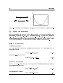
6.1 Schematic picture of pulling a lipid out of a lipid bilayer with AFM pulling.
Vrup is the velocity at which the spring is retracted, Zlink is the atom to
which the spring is attached and Zspring is the location of the spring. . . . . 98
6.2 Overview of the dierent reference group possibilities, applied to interface
systems. C is the reference group. The circles represent the center of mass
of 2 groups plus the reference group, and dc is the reference distance. . . . . 99
6.3 Dummy atom constructions for hydrogen atoms. . . . . . . . . . . . . . . . 104
6.4 Dummy atom constructions for aromatic residues. . . . . . . . . . . . . . . 105
8.1
8.2
8.3
8.4
8.5
8.6
8.7
8.8
8.9
8.10
8.11
8.12
8.13
The window of ngmx showing a box of water. . . . . . . . . . . . .
Denition of slices in g rdf. . . . . . . . . . . . . . . . . . . . . . .
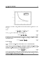
gOO (r) for Oxygen-Oxygen of SPC-water. . . . . . . . . . . . . . .
Mean Square Displacement of SPC-water. . . . . . . . . . . . . . .
Dihedral conventions. . . . . . . . . . . . . . . . . . . . . . . . . .
Options of g sgangle. . . . . . . . . . . . . . . . . . . . . . . . . .
A minimum distance matrix for a peptide [3]. . . . . . . . . . . . .
Geometrical Hydrogen bond criterion. . . . . . . . . . . . . . . . .
Insertion of water into an H-bond. . . . . . . . . . . . . . . . . . .
Analysis of the secondary structure elements of a peptide in time. .
Denition of the dihedral angles and of the protein backbone.
Ramachandran plot of a small protein. . . . . . . . . . . . . . . . .
Helical wheel projection of the N-terminal helix of HPr. . . . . . .
.
.
.
.
.
.
.
.
.
.
.
.
.
.
.
.
.
.
.
.
.
.
.
.
.
.
.
.
.
.
.
.
.
.
.
.
.
.
.
.
.
.
.
.
.
.
.
.
.
.
.
.
. 128
. 130
. 130
. 134
. 135
. 135
. 137
. 139
. 140
. 141
. 141
. 142
. 142
B.1 IEEE single precision oating point format . . . . . . . . . . . . . . . . . . 155
List of Tables
1.1 Typical vibrational frequencies. . . . . . . . . . . . . . . . . . . . . . . . . .
2.1
2.2
2.3
2.4
Basic units used in GROMACS . .
Derived units . . . . . . . . . . . .
Some Physical Constants . . . . .
Reduced Lennard-Jones quantities
.
.
.
.
.
.
.
.
.
.
.
.
.
.
.
.
.
.
.
.
.
.
.
.
.
.
.
.
.
.
.
.
.
.
.
.
.
.
.
.
.
.
.
.
.
.
.
.
.
.
.
.
.
.
.
.
.
.
.
.
.
.
.
.
.
.
.
.
.
.
.
.
.
.
.
.
.
.
.
.
.
.
.
.
.
.
.
.
.
.
.
.
3
10
10
11
11
3.1 The number of interactions between particles. . . . . . . . . . . . . . . . . . 35
4.1 Constants for Ryckaert-Bellemans potential (kJ mol;1 ). . . . . . . . . . . . 55
4.2 Parameters for the dierent functional forms of the non-bonded interactions. 66
5.1
5.2
5.3
5.4
Particle types in GROMACS . . . . . . . .
Static atom type properties in GROMACS
The topology (*.top) le, part 1. . . . . . .
The topology (*.top) le, part 2. . . . . . .
.
.
.
.
.
.
.
.
.
.
.
.
.
.
.
.
.
.
.
.
.
.
.
.
.
.
.
.
.
.
.
.
.
.
.
.
.
.
.
.
.
.
.
.
.
.
.
.
.
.
.
.
.
.
.
.
.
.
.
.
.
.
.
.
.
.
.
.
.
.
.
.
76
79
90
91
7.1 The GROMACS le types. . . . . . . . . . . . . . . . . . . . . . . . . . . . 110
B.1 List of C functions and their Fortran equivalent, plus the source les. . . . . 154
B.2 User specied potential function data. . . . . . . . . . . . . . . . . . . . . . 160
xvi
LIST OF TABLES
Chapter 1
Introduction.
1.1 Computational Chemistry and Molecular Modeling
GROMACS is an engine to perform molecular dynamics simulations and energy minimiza-
tion. These are two of the many techniques that belong to the realm of computational
chemistry and molecular modeling. Computational Chemistry is just a name to indicate
the use of computational techniques in chemistry, ranging from quantum mechanics of
molecules to dynamics of large complex molecular aggregates. Molecular modeling indicates the general process of describing complex chemical systems in terms of a realistic
atomic model, with the aim to understand and predict macroscopic properties based on
detailed knowledge on an atomic scale. Often molecular modeling is used to design new
materials, for which the accurate prediction of physical properties of realistic systems is
required.
Macroscopic physical properties can be distinguished in (a) static equilibrium properties,
such as the binding constant of an inhibitor to an enzyme, the average potential energy of a
system, or the radial distribution function in a liquid, and (b) dynamic or non-equilibrium
properties, such as the viscosity of a liquid, diusion processes in membranes, the dynamics
of phase changes, reaction kinetics, or the dynamics of defects in crystals. The choice of
technique depends on the question asked and on the feasibility of the method to yield
reliable results at the present state of the art. Ideally, the (relativistic) time-dependent
Schrodinger equation describes the properties of molecular systems with high accuracy,
but anything more complex than the equilibrium state of a few atoms cannot be handled
at this ab initio level. Thus approximations are mandatory; the higher the complexity
of a system and the longer the time span of the processes of interest is, the more severe
approximations are required. At a certain point (reached very much earlier than one would
wish) the ab initio approach must be augmented or replaced by empirical parameterization
of the model used. Where simulations based on physical principles of atomic interactions
still fail due to the complexity of the system (as is unfortunately still the case for the
prediction of protein folding; but: there is hope!) molecular modeling is based entirely
on a similarity analysis of known structural and chemical data. The QSAR methods
(Quantitative Structure-Activity Relations) and many homology-based protein structure
predictions belong to the latter category.
2
Introduction.
Macroscopic properties are always ensemble averages over a representative statistical ensemble (either equilibrium or non-equilibrium) of molecular systems. For molecular modeling this has two important consequences:
The knowledge of a single structure, even if it is the structure of the global energy
minimum, is not sucient. It is necessary to generate a representative ensemble at
a given temperature, in order to compute macroscopic properties. But this is not
enough to compute thermodynamic equilibrium properties that are based on free
energies, such as phase equilibria, binding constants, solubilities, relative stability of
molecular conformations, etc. The computation of free energies and thermodynamic
potentials requires special extensions of molecular simulation techniques.
While molecular simulations in principle provide atomic details of the structures
and motions, such details are often not relevant for the macroscopic properties of
interest. This opens the way to simplify the description of interactions and average
over irrelevant details. The science of statistical mechanics provides the theoretical
framework for such simplications. There is a hierarchy of methods ranging from
considering groups of atoms as one unit, describing motion in a reduced number of
collective coordinates, averaging over solvent molecules with potentials of mean force
combined with stochastic dynamics [4], to mesoscopic dynamics describing densities
rather than atoms and uxes as response to thermodynamic gradients rather than
velocities or accelerations as response to forces [5].
For the generation of a representative equilibrium ensemble two methods are available: (a)
Monte Carlo simulations and (b) Molecular Dynamics simulations. For the generation of
non-equilibrium ensembles and for the analysis of dynamic events, only the second method
is appropriate. While Monte Carlo simulations are more simple than MD (they do not
require the computation of forces), they do not yield signicantly better statistics than
MD in a given amount of computer time. Therefore MD is the more universal technique.
If a starting conguration is very far from equilibrium, the forces may be excessively large
and the MD simulation may fail. In those cases a robust energy minimization is required.
Another reason to perform an energy minimization is the removal of all kinetic energy
from the system: if several 'snapshots' from dynamic simulations must be compared,
energy minimization reduces the thermal 'noise' in the structures and potential energies,
so that they can be compared better.
1.2 Molecular Dynamics Simulations
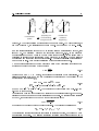
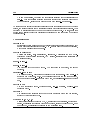
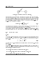
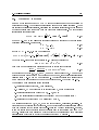
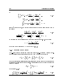
MD simulations solve Newton's equations of motion for a system of N interacting atoms:
mi @@tr2i = F i; i = 1 : : : N:
(1.1)
F i = ; @@Vri
(1.2)
2
The forces are the negative derivatives of a potential function V (r1 ; r 2 ; : : : ; rN ):
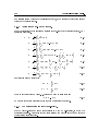
1.2 Molecular Dynamics Simulations
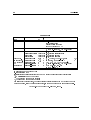
type of bond
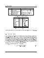
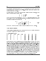
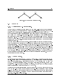
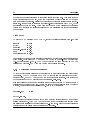
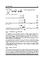
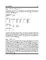
C-H, O-H, N-H
C=C, C=O,
HOH
C-C
H2 CX
CCC
O-H O
O-H O
3
type of
vibration
stretch
stretch
bending
stretch
sciss, rock
bending
libration
stretch
wavenumber
(cm;1 )
3000{3500
1700{2000
1600
1400{1600
1000{1500
800{1000
400{ 700
50{ 200
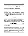
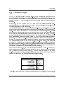
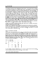
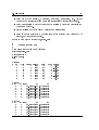
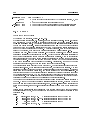
Table 1.1: Typical vibrational frequencies (wavenumbers) in molecules and hydrogenbonded liquids. Compare kT=h = 200 cm;1 at 300 K.
The equations are solved simultaneously in small time steps. The system is followed for
some time, taking care that the temperature and pressure remain at the required values,
and the coordinates are written to an output le at regular intervals. The coordinates as
a function of time represent a trajectory of the system. After initial changes, the system
will usually reach an equilibrium state. By averaging over an equilibrium trajectory many
macroscopic properties can be extracted from the output le.
It is useful at this point to consider the limitations of MD simulations. The user should be
aware of those limitations and always perform checks on known experimental properties
to assess the accuracy of the simulation. We list the approximations below.
The simulations are classical
Using Newton's equation of motion automatically implies the use of classical mechanics to describe the motion of atoms. This is all right for most atoms at normal
temperatures, but there are exceptions. Hydrogen atoms are quite light and the
motion of protons is sometimes of essential quantum mechanical character. For
example, a proton may tunnel through a potential barrier in the course of a transfer over a hydrogen bond. Such processes cannot be properly treated by classical
dynamics! Helium liquid at low temperature is another example where classical mechanics breaks down. While helium may not deeply concern us, the high frequency
vibrations of covalent bonds should make us worry! The statistical mechanics of a
classical harmonic oscillator diers appreciably from that of a real quantum oscillator, when the resonance frequency approximates or exceeds kB T=h. Now at room
temperature the wavenumber = 1= = =c at which h = kB T is approximately
200 cm;1 . Thus all frequencies higher than, say, 100 cm;1 are suspect of misbehavior in classical simulations. This means that practically all bond and bond-angle
vibrations are suspect, and even hydrogen-bonded motions as translational or librational H-bond vibrations are beyond the classical limit (see Table 1.1). What can
we do?
Well, apart from real quantum-dynamical simulations, we can do either of two things:
(a) If we perform MD simulations using harmonic oscillators for bonds, we should
4
Introduction.
make corrections to the total internal energy U = Ekin + Epot and specic heat CV
(and to entropy S and free energy A or G if those are calculated). The corrections to
the energy and specic heat of a one-dimensional oscillator with frequency are: [6]
(1.3)
U QM = U cl + kT 21 x ; 1 + ex x; 1
CVQM
= CVcl + k
!
x2ex ; 1 ;
(ex ; 1)2
(1.4)
where x = h=kT . The classical oscillator absorbs too much energy (kT ), while
the high-frequency quantum oscillator is in its ground state at the zero-point energy
level of 21 h .
(b) We can treat the bonds (and bond angles) as constraints in the equation of
motion. The rational behind this is that a quantum oscillator in its ground state
resembles a constrained bond more closely than a classical oscillator. A good practical reason for this choice is that the algorithm can use larger time steps when the
highest frequencies are removed. In practice the time step can be made four times
as large when bonds are constrained than when they are oscillators [7]. GROMACS
has this option for the bonds, and for the bond angles. The exibility of the latter
is rather essential to allow for the realistic motion and coverage of congurational
space [7].
Electrons are in the ground state
In MD we use a conservative force eld that is a function of the positions of atoms
only. This means that the electronic motions are not considered: the electrons are
supposed to adjust their dynamics innitely fast when the atomic positions change
(the Born-Oppenheimer approximation), and remain in their ground state. This
is really all right, almost always. But of course, electron transfer processes and
electronically excited states can not be treated. Neither can chemical reactions be
treated properly, but there are other reasons to shy away from reactions for the time
being.
Force elds are approximate
Force elds provide the forces. They are not really a part of the simulation method
and their parameters can be user-modied as the need arises or knowledge improves.
But the form of the forces that can be used in a particular program is subject
to limitations. The force eld that is incorporated in GROMACS is described in
Chapter 4. In the present version the force eld is pair-additive (apart from longrange coulomb forces), it cannot incorporate polarizabilities, and it does not contain
ne-tuning of bonded interactions. This urges the inclusion of some limitations in
this list below. For the rest it is quite useful and fairly reliable for bio macromolecules in aqueous solution!
The force eld is pair-additive
This means that all non-bonded forces result from the sum of non-bonded pair interactions. Non pair-additive interactions, the most important example of which is
interaction through atomic polarizability, are represented by eective pair potentials.
1.3 Energy Minimization and Search Methods
5
Only average non pair-additive contributions are incorporated. This also means that
the pair interactions are not pure, i.e., they are not valid for isolated pairs or for
situations that dier appreciably from the test systems on which the models were
parameterized. In fact, the eective pair potentials are not that bad in practice. But
the omission of polarizability also means that electrons in atoms do not provide a
dielectric constant as they should. For example, real liquid alkanes have a dielectric
constant of slightly more than 2, which reduce the long-range electrostatic interaction between (partial) charges. Thus the simulations will exaggerate the long-range
Coulomb terms. Luckily, the next item compensates this eect a bit.
Long-range interactions are cut-o
In this version GROMACS always uses a cut-o radius for the Lennard-Jones interactions and sometimes also for Coulomb. Due to the minimum-image convention
(only one image of each particle in the periodic boundary conditions is considered
for a pair interaction), the cut-o range can not exceed half the box size. That is
still pretty big for large systems, and trouble is only expected for systems containing charged particles. But then real bad things may happen, like accumulation of
charges at the cut-o boundary or very wrong energies! For such systems you should
consider using one of the implemented long-range electrostatic algorithms.
Boundary conditions are unnatural
Since system size is small (even 10,000 particles is small), a cluster of particles will
have a lot of unwanted boundary with its environment (vacuum). This we must
avoid if we wish to simulate a bulk system. So we use periodic boundary conditions,
to avoid real phase boundaries. But liquids are not crystals, so something unnatural
remains. This item is mentioned in the last place because it is the least evil of all.
For large systems the errors are small, but for small systems with a lot of internal
spatial correlation, the periodic boundaries may enhance internal correlation. In that
case, beware and test the inuence of system size. This is especially important when
using lattice sums for long-range electrostatics, since these are known to sometimes
introduce extra ordering.
1.3 Energy Minimization and Search Methods
As mentioned in sec. 1.1, in many cases energy minimization is required. GROMACS
provides a simple form of local energy minimization, the steepest descent method.
The potential energy function of a (macro)molecular system is a very complex landscape
(or hyper surface) in a large number of dimensions. It has one deepest point, the global
minimum and a very large number of local minima, where all derivatives of the potential
energy function with respect to the coordinates are zero and all second derivatives are
nonnegative. The matrix of second derivatives, which is called the Hessian matrix, has
nonnegative eigenvalues; only the collective coordinates that correspond to translation and
rotation (for an isolated molecule) have zero eigenvalues. In between the local minima there
are saddle points, where the Hessian matrix has only one negative eigenvalue. These points
are the mountain passes through which the system can migrate from one local minimum
6
Introduction.
to another.
Knowledge of all local minima, including the global one, and of all saddle points would
enable us to describe the relevant structures and conformations and their free energies, as
well as the dynamics of structural transitions. Unfortunately, the dimensionality of the
congurational space and the number of local minima is so high that it is impossible to
sample the space at a sucient number of points to obtain a complete survey. In particular,
no minimization method exists that guarantees the determination of the global minimum.
However, given a starting conguration, it is possible to nd the nearest local minimum.
Nearest in this context does not always imply nearest in a geometrical sense (i.e., the
least sum of square coordinate dierences), but means the minimum that can be reached
by systematically moving down the steepest local gradient. Finding this nearest local
minimum is all that GROMACS can do for you, sorry! If you want to nd other minima
and hope to discover the global minimum in the process, the best advice is to experiment
with temperature-coupled MD: run your system at a high temperature for a while and
then quench it slowly down to the required temperature; do this repeatedly! If something
as a melting or glass transition temperature exists, it is wise to stay for some time slightly
below that temperature and cool down slowly according to some clever scheme, a process
called simulated annealing. Since no physical truth is required, you can use your phantasy
to speed up this process. One trick that often works is to make hydrogen atoms heavier
(mass 10 or so): although that will slow down the otherwise very rapid motions of hydrogen
atoms, it will hardly inuence the slower motions in the system while enabling you to
increase the time step by a factor of 3 or 4. You can also modify the potential energy
function during the search procedure, e.g. by removing barriers (remove dihedral angle
functions or replace repulsive potentials by soft core potentials [8]), but always take care
to restore the correct functions slowly. The best search method that allows rather drastic
structural changes is to allow excursions into four-dimensional space [9], but this requires
some extra programming beyond the standard capabilities of GROMACS .
Three possible energy minimization methods are:
Those that require only function evaluations. Examples are the simplex method and
its variants. A step is made on the basis of the results of previous evaluations. If
derivative information is available, such methods are inferior to those that use this
information.
Those that use derivative information. Since the partial derivatives of the potential
energy with respect to all coordinates are known in MD programs (these are equal
to minus the forces) this class of methods is very suitable as modication of MD
programs.
Those that use second derivative information as well. These methods are superior
in their convergence properties near the minimum: a quadratic potential function is
minimized in one step! The problem is that for N particles a 3N 3N matrix must
be computed, stored and inverted. Apart from the extra programming to obtain
second derivatives, for most systems of interest this is beyond the available capacity.
There are intermediate methods building up the Hessian matrix on the y, but they
also suer from excessive storage requirements. So GROMACS will shy away from
1.3 Energy Minimization and Search Methods
7
this class of methods.
The steepest descent method, available in GROMACS , is of the second class. It simply
takes a step in the direction of the negative gradient (hence in the direction of the force),
without any consideration of the history built up in previous steps. The step size is
adjusted such that the search is fast but the motion is always downhill. This is a simple
and sturdy, but somewhat stupid, method: its convergence can be quite slow, especially in
the vicinity of the local minimum! The faster converging conjugate gradient method (see
e.g. [10]) uses gradient information from previous steps. In general, steepest descents will
bring you close to the nearest local minimum very quickly, while conjugate gradients brings
you very close to the local minimum, but performs worse far away from the minimum.
8
Introduction.
Chapter 2
Denitions and Units.
2.1 Notation
The following conventions for mathematical typesetting are used throughout this document:
Item
Notation Example
Vector
Bold italic
ri
Vector Length Italic
ri
We dene the lowercase subscripts i, j , k and l to denote particles: ri is the position vector
of particle i, and using this notation:
rij = rj ; ri
(2.1)
rij = jrij j
(2.2)
The force on particle i is denoted by F i and
F ij = force on i exerted by j
(2.3)
Please note that we changed notation as of ver. 2.0 to rij = rj ; ri since this is the
notation commonly used. If you encounter an error, let us know.
2.2 MD units
GROMACS uses a consistent set of units that produce values in the vicinity of unity for
most relevant molecular quantities. Let us call them MD units. The basic units in this
system are nm, ps, K, electron charge (e) and atomic mass unit (u), see Table 2.1.
Consistent with these units are a set of derived units, given in Table 2.2.
The electric conversion factor f = 4"1 o = 138:935 485(9) kJ mol;1 nm e;2 . It relates
the mechanical quantities to the electrical quantities as in
2
2
V = f qr or F = f rq2
(2.4)
10
Denitions and Units.
Quantity
length
mass
Symbol Unit
r
nm = 10;9 m
m
u (atomic mass unit) = 1.6605402(10)10;27 kg
(1/12 of the mass of a C atom)
1:6605402(10) 10;27 kg
time
t
ps = 10;12 s
charge
q
e = electronic charge = 1:60217733(49) 10;19 C
temperature
T
K
Table 2.1: Basic units used in GROMACS . Numbers in parentheses give accuracy.
Quantity
energy
Force
pressure
Symbol Unit
E; V kJ mol;1
F kJ mol;1 nm;1
p
kJ mol;1 nm;3 = 1030 =NAV Pa
1:660 54 106 Pa = 16:6054 Bar
velocity
v
nm ps;1 = 1000 m/s
dipole moment
e nm
electric potential
kJ mol;1 e;1 = 0:010 364 272(3) Volt
electric eld
E
kJ mol;1 nm;1 e;1 = 1:036 427 2(3) 107 V/m
Table 2.2: Derived units
Electric potentials and electric elds E are intermediate quantities in the calculation of
energies and forces. They do not occur inside GROMACS . If they are used in evaluations,
there is a choice of equations and related units. We recommend strongly to follow the
usual practice to include the factor f in expressions that evaluate and E :
X qj
j jr ; rj j
X
E (r) = f qj j(rr;;rrjjj)3
j
(r) = f
(2.5)
(2.6)
With these denitions q is an energy and qE is a force. The units are those given in
Table 2.2: about 10 mV for potential. Thus the potential of an electronic charge at a
distance of 1 nm equals f 140 units 1:4 V. (exact value: 1.439965 V)
Note that these units are mutually consistent; changing any of the units is likely to produce
inconsistencies and is therefore strongly discouraged ! In particular: if A are used instead
of nm, the unit of time changes to 0.1 ps. If the kcal/mol (= 4.184 kJ/mol) is used instead
of kJ/mol for energy, the unit of time becomes 0.488882 ps and the unit of temperature
changes to 4.184 K. But in both cases all electrical energies go wrong, because they will still
be computed in kJ/mol, expecting nm as the unit of length. Although careful rescaling of
charges may still yield consistency, it is clear that such confusions must be rigidly avoided.
In terms of the MD units the usual physical constants take on dierent values, see Table 2.3.
All quantities are per mol rather than per molecule. There is no distinction between
2.3 Reduced units
11
Symbol Name
NAV Avogadro's number
R
gas constant
kB
Boltzmann's constant
h
Planck's constant
h
Dirac's constant
c
velocity of light
Value
6:022 136 7(36) 1023 mol;1
8:314 510(70) 10;3 kJ mol;1 K;1
idem
0:399 031 32(24) kJ mol;1 ps
0:063 507 807(38) kJ mol;1 ps
299 792:458 nm/ps
Table 2.3: Some Physical Constants
Quantity
Symbol Relation to SI
Length
r
r ;1
Mass
m
m M;1p
Time
t
t ;1 =M
Temperature
T
kB T ;1
Energy
E
E ;1
Force
F
F ;1
Pressure
P
Pp
3 ;1
Velocity
v
v M=
Density
N 3 V ;1
Table 2.4: Reduced Lennard-Jones quantities
Boltzmann's constant k and the gas constant R: their value is 0:008 314 51 kJ mol;1 K;1 .
2.3 Reduced units
When simulating Lennard-Jones (LJ) systems it might be advantageous to use reduced
units (i.e., setting ii = ii = mi = kB = 1 for one type of atoms). This is possible. When
specifying the input in reduced units, the output will also be in reduced units. There is
one exception: the temperature, which is expressed in 0:008 314 51 reduced units. This
is a consequence of the use of Boltzmann's constant in the evaluation of temperature in
the code. Thus not T , but kB T is the reduced temperature. A GROMACS temperature
T = 1 means a reduced temperature of 0.008. . . units; if a reduced temperature of 1 is
required, the GROMACS temperature should be 120.2717.
In Table 2.4 quantities are given for LJ potentials:
" 12 6 #
VLJ = 4 r ; r
(2.7)
12
Denitions and Units.
Chapter 3
Algorithms
3.1 Introduction
In this chapter we rst give describe two general concepts used in GROMACS : periodic
boundary conditions (sec. 3.2) and the group concept (sec. 3.3). The MD algorithm is
described in sec. 3.4: rst a global form of the algorithm is given, which is rened in
subsequent subsections. The (simple) EM (Energy Minimization) algorithm is described
in sec. 3.7. Some other algorithms for special purpose dynamics are described after this.
In the nal sec. 3.11 of this chapter a few principles are given on which parallelization of
GROMACS is based. The parallelization is hardly visible for the user and is therefore not
treated in detail.
A few issues are of general interest. In all cases the system must be dened, consisting
of molecules. Molecules again consist of particles with dened interaction functions. The
detailed description of the topology of the molecules and of the force eld and the calculation of forces is given in chapter 4. In the present chapter we describe other aspects of
the algorithm, such as pair list generation, update of velocities and positions, coupling to
external temperature and pressure, conservation of constraints. The analysis of the data
generated by an MD simulation is treated in chapter 8.
3.2 Periodic boundary conditions
The classical way to minimize edge eects in a nite system is to apply periodic boundary
conditions. The atoms of the system to be simulated are put into a space-lling box,
which is surrounded by translated copies of itself (Fig. 3.1). Thus there are no boundaries
of the system; the artifact caused by unwanted boundaries in an isolated cluster is now
replaced by the artifact of periodic conditions. If a crystal is simulated, such boundary
conditions are desired (although motions are naturally restricted to periodic motions with
wavelengths tting into the box). If one wishes to simulate non-periodic systems, as
liquids or solutions, the periodicity by itself causes errors. The errors can be evaluated
by comparing various system sizes; they are expected to be less severe than the errors
resulting from an unnatural boundary with vacuum.
14
Algorithms
i’
i’
i’
i’
i
i’
j
i’
i’
Rc
i’
Figure 3.1: Periodic boundary conditions in two dimensions.
There are several possible shapes for space-lling unit cells. Some, as the truncated octahedron [11] approach a spherical shape better than a cubic box and are therefore more
economical for studying an (approximately spherical) macromolecule in solution, since
less solvent molecules are required to ll the box given a minimum distance between
macromolecular images. However, a periodic system based on the truncated octahedron is
equivalent to a periodic system based on a triclinic unit cell. The latter shape is the most
general space-lling unit cell; it comprises all possible space-lling shapes [12]. Therefore
GROMACS will in future versions be based on the triclinic unit and will not contain other
unit cell shapes. However, in the present version only rectangular boxes are allowed.
GROMACS uses periodic boundary conditions, combined with the minimum image convention: only one - the nearest - image of each particle is considered for short-range
non-bonded interaction terms. For long-range electrostatic interactions this is not always
accurate enough, and GROMACS therefore also incorporates lattice sum methods like
Ewald Sum, PME and PPPM.
The box can be of arbitrary dimensions, but must be rectangular. An isolated cluster
of molecules can of course be simulated as well within these restrictions by dening the
periodic box size to be much larger than the cluster size.
The minimum image convention implies that the cut-o radius used to truncate nonbonded interactions must not exceed half the smallest box size:
Rc < 21 min(a; b; c);
(3.1)
otherwise more than one image would be within the cut-o distance of the force. When
a macromolecule, such as a protein, is studied in solution, this restriction does not sufce. In principle a single solvent molecule should not be able to `see' both sides of the
macromolecule. This means that an edge a of the box must exceed the length of the
3.3 The group concept
15
macromolecule in the direction of that edge plus two times the cut-o radius Rc . It is
common to compromise in this respect, and make the solvent layer somewhat smaller in
order to reduce the computational cost.
Each unit cell (cubic, rectangular or triclinic, the latter not being implemented in GROMACS ) is surrounded by 26 translated images. Thus a particular image can always be
identied by an index pointing to one of 27 translation vectors and constructed by applying
a translation with the indexed vector (see 3.4.2).
3.3 The group concept
In the GROMACS MD and analysis programs one uses groups of atoms to perform certain
actions on. The maximum number of groups is 256, but every atom can only belong to
four dierent groups, one of each of the following kinds:
T-coupling group The temperature coupling parameters (reference temperature, time
constant, number of degrees of freedom, see 3.4.3) can be dened for each T-coupling
group separately. For example, in a solvated macromolecule the solvent (that tends
to produce more heating by force and integration errors) can be coupled with a
shorter time constant to a bath than a macromolecule, or a surface can be kept cooler
than an adsorbing molecule. Many dierent T-coupling groups may be dened.
Freeze group Atoms that belong to a freeze group are kept stationary in the dynamics.
This is useful during equilibration, e.g. to avoid that badly placed solvent molecules
will give unreasonable kicks to protein atoms, although the same eect can also be
obtained by putting a restraining potential on the atoms that must be protected.
The freeze option can be used on one or two coordinates of an atom, thereby freezing
the atoms in a plane or on a line. Many freeze groups can be dened.
Accelerate group On each atom in an 'accelerate group' an acceleration ag will be
imposed. This is equivalent to an external force. This feature makes it possible to
drive the system into a non-equilibrium state and enables to perform non-equilibrium
MD to obtain transport properties.
Energy monitor group Mutual interactions between all energy monitor groups are
compiled during the simulation. This is done for Lennard Jones and Coulomb terms
separately. In principle up to 256 groups could be dened, but that would lead to
256256 items! Better use this concept sparingly.
The use of groups in analysis programs is described in chapter 8.
3.4 Molecular Dynamics
A global ow scheme for MD is given in Fig. 3.2. Each MD or EM run requires as input a
set of initial coordinates and - optionally - initial velocities of all particles involved. This
chapter does not describe how these are obtained; for the setup of an actual MD run check
the online manual at http://md.chem.rug.nl/~gmx.
16
Algorithms
THE GLOBAL MD ALGORITHM
1. Input initial conditions
Potential interaction V as a function of atom positions
Positions r of all atoms in the system
Velocities v of all atoms in the system
+
repeat 2,3,4 required number of steps:
2. Compute forces
The force on any atom
F i = ; @@Vri
is computed by calculating the force between non-bonded
atom pairs:
F i = Pj F ij
plus the forces due to bonded interactions (which may depend
on 1, 2, 3, or 4 atoms), plus restraining and/or external forces.
The potential and kinetic energies and the pressure tensor are
computed.
+
3. Update conguration
The movement of the atoms is simulated by numerically
solving Newton's equations of motion
d2 ri = F i
dt2 or mi
dri = v ; dvi = F i
i dt
dt
m
i
+
4. if required: Output step
write positions, velocities, energies, temperature, pressure, etc.
Figure 3.2: The global MD algorithm
17
Probability
3.4 Molecular Dynamics
0.0
0
Velocity
Figure 3.3: A Maxwellian distribution, generated from random numbers.
3.4.1 Initial conditions
Topology and force eld
The system topology, including a description of the force eld, must be loaded. These
items are described in chapter 4. All this information is static; it is never modied during
the run.
Coordinates and velocities
Then, before a run starts, the box size and the coordinates and velocities of all particles
are required. The box size is determined by three vectors (nine numbers) b1 ; b2 ; b3 , which
represent the three basis vectors of the periodic box. While in the present version of
GROMACS only rectangular boxes are allowed, three numbers suce, but the use of
three vectors already prepares for arbitrary triclinic boxes to be implemented in a later
version.
If the run starts at t = t0 , the coordinates at t = t0 must be known. The leap-frog
algorithm, used to update the time step with t (see 3.4.3), requires that the velocities
must be known at t = t0 ; 2t . If velocities are not available, the program can generate
initial atomic velocities vi ; i = 1 : : : 3N from a Maxwellian distribution (Fig. 3.3) at a given
absolute temperature T :
r m
i exp(; mi vi2 )
p(vi) = 2kT
(3.2)
2kT
where k is Boltzmann's constant (see chapter 2). To accomplish this, normally distributed
random numbers are generated by adding twelve random numbers Rk in the range 0 Rk < 1 and subtracting 6.0 from their psum. The result is then multiplied by the standard
deviation of the velocity distribution kT=mi . Since the resulting total energy will not
correspond exactly to the required temperature T , a correction is made: rst the centerof-mass motion is removed and then all velocities are scaled such that the total energy
18
Algorithms
corresponds exactly to T (see eqn. 3.10).
Center-of-mass motion
The center-of-mass velocity is normally set to zero at every step. Normally there is no
net external force acting on the system and the center-of-mass velocity should remain
constant. In practice, however, the update algorithm develops a very slow change in the
center-of-mass velocity, and thus in the total kinetic energy of the system, specially when
temperature coupling is used. If such changes are not quenched, an appreciable center-ofmass motion develops eventually in long runs, and the temperature will be signicantly
misinterpreted. The same may happen due to overall rotational motion, but only when an
isolated cluster is simulated. In periodic systems with lled boxes, the overall rotational
motion is coupled to other degrees of freedom and does not give any problems.
3.4.2 Compute forces
As mentioned in chapter 4, internal forces are either generated from xed (static) lists,
or from dynamics lists. The latter concern non-bonded interactions between any pair of
particles.
Pair lists generation
The non-bonded pair forces need to be calculated only for those pairs i; j for which the
distance rij between i and the nearest image of j is less than a given cut-o radius rc . Some
of the particle pairs that fulll this criterion are excluded, when their interaction is already
fully accounted for by bonded interactions. GROMACS employs a pair list that contains
those particle pairs for which non-bonded forces must be calculated. The pair list contains
the particle numbers and an index for the image displacement vectors that must be applied
to obtain the nearest image, for all particle pairs that have a nearest-image distance less
than rshort. The list is updated every nstlist steps, where nstlist is typically 10 or
20. There is an option to calculate the total non-bonded force on each particle due to
all particle in a shell around the list-cuto, i.e, at a distance between rshort and rlong.
This force is calculated during the pair list update and retained during nstlist steps.
The vector rij = rj ; ri connecting nearest images is found by constructing
xij = xij ; a round(xij =a)
(3.3)
yij = yij ; b round(yij =b)
(3.4)
zij = zij ; c round(zij =c)
(3.5)
where the length of the box edges are denoted by a; b; c, and the function round(x) delivers
the integer number that is nearest to x. The translation vector index is determined by the
27 combinations of the -1, 0, or +1 values of the three round function results (assuming
that all primary particles are in the central box).
The particles will move during the simulation, and may move outside the primary box.
Before a new pair list is made up, all particles will be reset to the primary box, which lies
3.4 Molecular Dynamics
19
X
0
1
2
3
4
5
0
1
Y
2
3
4
j
i
k
5
Figure 3.4: The computational box in two dimensions, divided into NS grid cells with
three particles, i, j and k. Each NS grid cell is of size rc =2.
in the positive quadrant with respect to an origin at r0 , by applying
xi = xi ; a round([xi ; x0 ; a=2]=a)
yi = yi ; b round([yi ; y0 ; b=2]=b)
zi = zi ; c round([zi ; z0 ; c=2]=c)
(3.6)
(3.7)
(3.8)
Image calculation on a grid.
GROMACS uses an interaction list for non-bonded interactions, usually called the neighbor
list. This list is made every nstlist MD steps, where nstlist is typically 10 MD steps.
To make the neighbor list all particles that are close (i.e. within the cut-o) to a given
particle must be found. This searching, usually called neighbor searching (NS), involves
periodic boundary conditions and determining the image (see sec. 3.2). When the cut-o
is large compared to the box edge l (> 0.4l) searching is done using an O(N 2 ) algorithm
that computes all distances and compares them to the cut-o rc. When the cut-o is
smaller than 0.4l in all directions (x,y and z) searching is done using a grid, the NS
grid. All particles are put on the NS grid, with the smallest spacing rc=2 in each of
the directions 1 . We have depicted the computational box, divided into NS grid cells in
Fig. 3.4. In each spatial dimension, a particle i has three images. For each direction the
image may be -1,0 or 1, corresponding to a translation over -1, 0 or +1 box vector. We do
not search the surrounding NS grid cells for neighbors of i and then calculate the image, but
rather construct the images rst and then search neighbors corresponding to that image
of i. Since we demand that the number of NS grid cells 5 in each direction the same
neighbor will not be found twice. For every particle, exactly 125 (53 ) neighboring cells are
searched. Therefore, the algorithm scales linear with the number of particles. Although
1 In fact the cut-o is divided into sub-blocks, the number of which can be chosen by the user. The
default for this number (grid ) is 2, such that the NS grid spacing must be rc=2. For simplicity we will
just use this particular choice in the remainder of the text. However, it can be easily understood that if
grid = 3, we need at least 2grid = 7 grid-cells, each of which has size rc =3
20
Algorithms
the prefactor is large (125) the scaling behavior makes the algorithm far superior over the
standard O(N 2 ) algorithm when the number of particles exceeds a few hundred.
In the example of Fig. 3.4 the image tx = 0 of particle i will nd j as a neighbor, while
image tx = 1 of particle i will nd k as a neighbor.
Charge groups
Where applicable, neighbor searching is carried out on the basis of charge groups. A charge
group is a small set of nearby atoms that have net charge zero. Charge groups are dened
in the molecular topology. If the nearest image distance between the geometrical centers
of the atoms of two charge groups is less than the cuto radius, all atom pairs between the
charge groups are included in the pair list. This procedure avoids the creation of charges
due to the use of a cut-o (when one charge of a dipole is within range and the other
not), which can have disastrous consequences for the behavior of the Coulomb interaction
function at distances near the cut-o radius. If molecular groups have full charges (ions),
charge groups do not avoid adverse cut-o eects, and you should consider using one of
the lattice sum methods supplied by GROMACS [13].
If appropriately constructed shift functions are used for the electrostatic forces, no charge
groups are needed. Such shift functions are implemented in GROMACS (see chapter 4)
but must be used with care: in principle they should be combined with a lattice sum for
long-range electrostatics.
The actual neighbor search is performed on a grid. The details of the algorithm are not
relevant for the user and are not given here.
Potential energy
When forces are computed, the potential energy of each interaction term is computed as
well. The total potential energy is summed for various contributions, such as Lennard
Jones, Coulomb, and bonded terms. It is also possible to compute these contributions for
groups of atoms that are separately dened (see sec. 3.3).
Kinetic energy and temperature
The temperature is given by the total kinetic energy of the N -particle system:
Ekin = 21
N
X
i=1
mi vi2
(3.9)
From this the absolute temperature T can be computed using:
1
(3.10)
2 Ndf kT = Ekin
where k is Boltzmann's constant and Ndf is the number of degrees of freedom which can
be computed from:
Ndf = 3N ; Nc ; 3
(3.11)
3.4 Molecular Dynamics
21
x
v
0
x
1
2
t
Figure 3.5: The Leap-Frog integration method. The algorithm is called Leap-Frog (Haasje
Over), because r and v are leaping like frogs over each others back.
Here Nc is the number of constraints imposed on the system. The additional 3 degrees of
freedom must be removed because the three center-of-mass velocities are constants of the
motion, which are usually set to zero. This correction is small; in the current version of
GROMACS it is ignored.
The kinetic energy can also be written as a tensor, which is necessary for pressure calculation in a triclinic system, or systems where shear forces are imposed:
N
X
(3.12)
Ekin = 12 mivi vi
i
Pressure and virial
The pressure tensor P is calculated from the dierence between kinetic energy Ekin and
the virial (3.13)
P = 32V (Ekin ; )
where V is the volume of the computational box. The scalar pressure P , which can be
used for pressure coupling in the case of isotropic systems, is computed as:
P = trace(P)=3
(3.14)
The virial tensor is dened as
= ; 12
X
i<j
rij F ij
(3.15)
In sec. B.1 the implementation in GROMACS of the virial computation is described.
3.4.3 Update conguration
The GROMACS MD program utilizes the so-called leap-frog algorithm [14] for the integration of the equations of motion. The leap-frog algorithm uses positions r at time t
and velocities v at time t ; 2t ; it updates positions and velocities using the forces F (t)
determined by the positions at time t:
v(t + 2t ) = v(t ; 2t ) + Fm(t) t
(3.16)
r(t + t) = r(t) + v(t + 2t )t
(3.17)
22
Algorithms
The algorithm is visualized in Fig. 3.5. It is equivalent to the Verlet [15] algorithm:
r(t + t) = 2r(t) ; r(t ; t) + Fm(t) t2 + O(t4)
(3.18)
The algorithm is of third order in r and is time-reversible. See ref. [16] for the merits of
this algorithm and comparison with other time integration algorithms.
The equations of motion are modied for temperature coupling and pressure coupling, and
extended to include the conservation of constraints, all of which are described below.
Temperature coupling
For several reasons (drift during equilibration, drift as a result of force truncation and
integration errors, heating due to external or frictional forces), it is necessary to control
the temperature of the system. GROMACS uses the weak coupling scheme [17] that mimics
weak coupling with rst-order kinetics to an external heat bath with given temperature
T0 . See ref [18] for a comparison of this temperature control method with the Nose-Hoover
scheme [19, 20]. The eect of the algorithm is that a deviation of the system temperature
from T0 is slowly corrected according to
dT = T0 ; T
(3.19)
dt
which means that a temperature deviation decays exponentially with a time constant .
This method of coupling has the advantage that the strength of the coupling can be varied
and adapted to the user requirement: for equilibration purposes the coupling time can be
taken quite short (e.g. 0.01 ps), but for reliable equilibrium runs it can be taken much
longer (e.g. 0.5 ps) in which case it hardly inuences the conservative dynamics.
The heat ow into or out of the system is eected by scaling the velocities of each particle
every step with a time-dependent factor , given by
"
t
= 1+ T
(
T0
T (t ; 2t )
;1
)#1=2
(3.20)
The parameter T is close to, but not exactly equal to the time constant of the temperature coupling (eqn. 3.19):
= 2CV T =Ndf k
(3.21)
where CV is the total heat capacity of the system, k is Boltzmann's constant, and Ndf
is the total number of degrees of freedom. The reason that 6= T is that the kinetic
energy change caused by scaling the velocities is partly redistributed between kinetic and
potential energy and hence the change in temperature is less than the scaling energy. In
practice, the ratio =T ranges from 1 (gas) to 2 (harmonic solid) to 3 (water). When
we use the term 'temperature coupling time constant', we mean the parameter T . Note
that in practice the scaling factor is limited to the range of 0.8 <= <= 1.25, to avoid
scaling by very large numbers which may crash the simulation. In normal use, will
always be much closer to 1.0.
3.4 Molecular Dynamics
23
Strictly, for computing the scaling factor the temperature T is needed at time t, but this
is not available in the algorithm. In practice, the temperature at the previous time step
is used (as indicated in eqn. 3.20), which is perfectly all right since the coupling time
constant is much longer than one time step. The algorithm is stable up to T t.
Pressure coupling
In the same spirit as the temperature coupling, the system can also be coupled to a
'pressure bath'. This is accomplished [17] by scaling coordinates and box size every step
with a parameter , which has the eect of a rst-order kinetic relaxation of the pressure
towards a given reference pressure P0 :
dP = P0 ; P
(3.22)
dt
p
The scaling factor is given by
"
#1=3
t
= 1 + fP (t) ; P0 g
p
(3.23)
Here is the isothermal compressibility of the system. In general this is not known. It
suces to take a rough estimate because the value of only inuences the non-critical
time constant of the pressure relaxation without aecting the average pressure itself. For
water at 1 atm and 300 K = 4:5 10;10 Pa;1 = 4:5 10;5 Bar;1 , which is 7:5 10;4
MD units (see chapter 2). Most other liquids have similar values.
In the present version of GROMACS the pressure coupling can be done anisotropically:
the x; y; z dimensions are scaled separately, based on the diagonal elements of the pressure
tensor. This allows e.g. to couple one dimension to an external pressure, while keeping a
xed surface area in the other two dimensions (useful in membrane simulations). The system axes remain orthogonal (the scaling method allows in principle also dynamic changes
in box angles, but this is not implemented yet).
Since the pressure uctuates heavily, it is recommended to take p not too small; a value
between 0.4 and 1 ps will often be satisfactory. When using lattice sum methods it is
easy to get pressure oscillations, but this can be overcome by either slower scaling or by
averaging the calculated pressure over several steps.
Surface tension coupling
When a periodic system consists of more than one phase, separated by surfaces which are
parallel to the xy-plane, the surface tension and the z-component of the pressure can be
coupled to a pressure bath. The average surface tension (t) can be calculated from the
dierence between the normal and the lateral pressure:
Z Lz Pz (z; t) ; Px (z; t) +2 Py (z; t) dz
(3.24)
(t) = n1
0
L
P
(
t
)
+
P
(
t
)
z
x
y
= n Pz (t) ;
(3.25)
2
24
Algorithms
where Lz is the height of the box and n is the number of surfaces. The pressure in the
z-direction is corrected by scaling the height of the box with z :
P = t fP ; P (t)g
(3.26)
z
p
z0
z
z = 1 + z Pz
(3.27)
This is similar to normal pressure coupling, except that the power of one third is missing.
The pressure correction in the z-direction is then used to get the correct convergence for
the surface tension to the reference value 0 . The correction factor for the box-length in
the x/y-direction is:
"
n0 # 12
t
P
(
t
)
+
P
(
t
)
x
y
xy = 1 + xy L ; Pz (t) + Pz ;
2
p
z z
(3.28)
The value of z is more critical than with normal pressure coupling. Normally an incorrect
compressibility will just scale p , but with surface tension coupling it aects the convergence of the surface tension. When z is set to zero (constant box height), Pz is also set
to zero, which is necessary for obtaining the correct surface tension.
The complete update algorithm
The complete algorithm for the update of velocities and coordinates is given in Fig. 3.6.
The SHAKE algorithm of step 4 is explained below.
GROMACS has a provision to "freeze" (prevent motion of) selected particles, which must
be dened as a 'freeze group'. This is implemented using a freeze factor f g , which is a
vector, and diers for each freezegroup (see sec. 3.3). This vector contains only zero (freeze)
or one (don't freeze). When we take this freeze factor and the external acceleration ah
into account the update algorithm for the velocities becomes:
t
F
(
t
)
t
(3.29)
v(t + 2 ) = f g v(t ; 2 ) + m t + aht
where g and h are group indices which dier per atom.
3.4.4 Constraint algorithms
SHAKE
Constraints can be imposed in GROMACS using the traditional0 SHAKE method [21].
The SHAKE routine changes a set of unconstrained coordinates r to a set of coordinates
r00 that fulll a list of distance constraints, using a set r as reference:
SHAKE(r0 ! r00 ; r)
This action is consistent with solving a set of Lagrange multipliers in the constrained
equations of motion. SHAKE needs a tolerance TOL; it will continue until all constraints
3.4 Molecular Dynamics
25
THE UPDATE ALGORITHM
Given:
Positions r of all atoms at time t
Velocities v of all atoms at time t ; 2t
Accelerations F =m on all atoms at time t.
(Forces are computed disregarding any constraints)
Total kinetic energy and virial
+
1. Compute the scaling factors and according to eqns. 3.20 and 3.23
+
2. Update and scale velocities: v0 = (v + at)
+
3. Compute new unconstrained coordinates: r0 = r + v0t
+
4. Apply constraint algorithm
to coordinates:
constrain(r0 ! r00 ; r)
+
5. Correct velocities for constraints: v = (r00 ; r)=t
+
6. Scale coordinates and box: r = r00; b = b
Figure 3.6: The MD update algorithm
26
Algorithms
are satised within a relative tolerance TOL. An error message is given if SHAKE cannot
reset the coordinates because the deviation is too large, or if a given number of iterations
is surpassed.
Assume the equations of motion must fulll K holonomic constraints, expressed as
k (r1 : : : rN ) = 0; k = 1 : : : K
(3.30)
(e.g. (r1 ; r2 )2 ; b2 = 0). Then the forces are dened as
K
X
; @@r V + k k
i
k=1
!
(3.31)
where k are Lagrange multipliers which must be solved to fulll the constraint equations.
The second part of this sum determines the constraint forces Gi , dened by
Gi = ;
K
X
@k
k=1
k @r
(3.32)
i
The displacement due to the constraint forces in the leap frog or Verlet algorithm is
equal to (Gi =mi )(t)2 . Solving the Lagrange multipliers (and hence the displacements)
requires the solution of a set of coupled equations of the second degree. These are solved
iteratively by SHAKE. For the special case of rigid water molecules, that often make up
more than 80% of the simulation system we have implemented the SETTLE algorithm [22]
(sec. B.2.2).
The LINCS algorithm
LINCS is an algorithm that resets bonds to their correct lengths after an unconstrained
update [23]. The method is non-iterative, as it always uses two steps. Although LINCS
is based on matrices, no matrix-matrix multiplications are needed. The method is more
stable and faster than SHAKE, but it can only be used with bond constraints and isolated
angle constraints, such as the proton angle in OH. Because of its stability LINCS is
especially useful for Langevin Dynamics. LINCS has two parameters, which are explained
in the subsection parameters.
The LINCS formulas
We consider a system of N particles, with positions given by a 3N vector r(t). For
Molecular Dynamics the equations of motion are given by Newton's law
d2 r = M ;1 F
(3.33)
dt2
where F is the 3N force vector and M is a 3N 3N diagonal matrix, containing the masses
of the particles. The system is constrained by K time-independent constraint equations
gi (r) = jri1 ; ri2 j ; di = 0
i = 1; : : : ; K
(3.34)
3.4 Molecular Dynamics
27
θ
l
d
d
unconstrained
update
p
d
projecting out
forces working
along the bonds
correction for
rotational
lengthening
Figure 3.7: The three position updates needed for one time step. The dashed line is 1the
old bond of length d, the solid lines are the new bonds. l = d cos and p = (2d2 ; l2 ) 2 .
In a numerical integration scheme LINCS is applied after an unconstrained update, just
like SHAKE. The algorithm works in two steps (see gure Fig. 3.7). In the rst step
the projections of the new bonds on the old bonds are set to zero. In the second step a
correction is applied for the lengthening of the bonds due to rotation. The numerics for
the rst step and the second step are very similar. A complete derivation of the algorithm
can be found in [23]. Only a short description of the rst step is given here.
A new notation is introduced for the gradient matrix of the constraint equations which
appears on the right hand side of the equation
h
Bhi = @g
@r
i
(3.35)
Notice that B is a K 3N matrix, it contains the directions of the constraints. The
following equation shows how the new constrained coordinates rn+1 are related to the
unconstrained coordinates runc
n+1
rn+1 = (I ; T nBn)runc
n+1 + T n d =
(3.36)
;1
;1 T ;1
unc
runc
n+1 ; M B n (B n M B n ) (B n rn+1 ; d)
where T = M ;1 B T (BM ;1 B T );1 . The derivation of this equation from eqns. 3.33 and
3.34 can be found in [23].
This rst step does not set the real bond lengths to the prescribed lengths, but the projection of the new bonds onto the old directions of the bonds. To correct for the rotation
of bond i, the projection of the bond on the old direction is set to
q
pi = 2d2i ; li2
(3.37)
where li is the bond length after the rst projection. The corrected positions are
rn+1 = (I ; T nB n)rn+1 + T np
(3.38)
This correction for rotational eects is actually an iterative process, but during MD only
one iteration is applied. The relative constraint deviation after this procedure will be
28
Algorithms
less than 0.0001 for every constraint. In energy minimization this might not be accurate
enough, so the number of iterations is equal to the order of the expansion (see below).
Half of the CPU time goes to inverting the constraint coupling matrix B n M ;1 B Tn , which
has to be done every time step. This K K matrix has 1=mi1 +1=mi2 on the diagonal. The
o-diagonal elements are only non-zero when two bonds are connected, then the element
is cos =mc , where mc is the mass of the atom connecting the two bonds and is the angle
between the bonds.
The matrix T is inverted through a power expansion. A K K matrix S is introduced
which is the inverse square root of the diagonal of B n M ;1 B Tn . This matrix is used to
convert the diagonal elements of the coupling matrix to one
(B n M ;1 B Tn );1 = SS ;1 (B n M ;1 B Tn );1 S ;1 S
= S (SB n M ;1 B Tn S );1 S = S (I ; An );1 S
(3.39)
(I ; An );1 = I + An + A2n + A3n + : : :
(3.40)
The matrix An is symmetric and sparse and has zeros on the diagonal. Thus a simple
trick can be used to calculate the inverse
This inversion method is only valid if the absolute values of all the eigenvalues of An
are smaller than one. In molecules with only bond constraints the connectivity is so low
that this will always be true, even if ring structures are present. Problems can arise in
angle-constrained molecules. By constraining angles with additional distance constraints
multiple small ring structures are introduced. This gives a high connectivity, leading to
large eigenvalues. Therefore LINCS should NOT be used with coupled angle-constraints.
The LINCS Parameters
The accuracy of LINCS depends on the number of matrices used in the expansion eqn. 3.40.
For MD calculations a fourth order expansion is enough. For Position Langevin Dynamics
with large time steps an eighth order expansion may be necessary. The order is a parameter
in the input le for mdrun. The implementation of LINCS is done in such a way that the
algorithm will never crash. Even when it is impossible to to reset the constraints LINCS
will generate a conformation which fullls the constraints as well as possible. However,
LINCS will generate a warning when in one step a bond rotates over more than a predened
angle. This angle is set by the user in the input le for mdrun.
3.4.5 Output step
The important output of the MD run is the trajectory le name.trj which contains particle
coordinates and -optionally- velocities at regular intervals. Since the trajectory les are
lengthy, one should not save every step! To retain all information it suces to write a
frame every 15 steps, since at least 30 steps are made per period of the highest frequency
in the system, and Shannon's sampling theorem states that two samples per period of
the highest frequency in a band-limited signal contain all available information. But
3.5 Simulated Annealing
29
that still gives very long les! So, if the highest frequencies are not of interest, 10 or
20 samples per ps may suce. Be aware of the distortion of high-frequency motions by
the stroboscopic eect, called aliasing: higher frequencies are mirrored with respect to the
sampling frequency and appear as lower frequencies.
3.5 Simulated Annealing
The well known simulated annealing (SA) protocol is implemented in a simple way into
GROMACS . A modication of the temperature coupling scheme is used as a very basic implementation of the SA algorithm. The method works as follows: the reference
temperature for coupling T0 (eqn. 3.19) is not constant but can be varied linearly:
T0 (step) = T0 (0 + step)
(3.41)
if 0 = 1 and is 0 this is the plain MD algorithm. Note that for standard SA must be negative. When T0 (step) < 0 it is set to 0, as negative temperatures do not have
a physical meaning. This \feature" allows for an annealing strategy in which at rst the
temperature is scaled down linearly until 0 K, and when more steps are taken the simulation proceeds at 0 K. Since the weak coupling scheme does not couple instantaneously,
the actual temperature will always be slightly higher than 0 K.
3.6 Langevin Dynamics
The Position Langevin Dynamics algorithm is implemented in GROMACS is (note: NOT
Velocity Langevin Dynamics). This applies to over-damped systems, i.e. systems in which
the inertia eects are negligible. The equations are
dr = F (r) + r
(3.42)
dt
where is the friction coecient [amu/ps] and r (t) is a noise process with hr i (t) rj (0)i =
2(t)ij kb T= . In GROMACS the equations are integrated with an explicit scheme
s
rn+1 = rn + t F (rn) + 2kb T t rG
(3.43)
where rG is Gaussian distributed noise with = 0, = 1. Because the system is assumed
to be over damped, large time-steps can be used. LINCS should be used for the constraints
since SHAKE will not converge for large atomic displacements. LD is an option of the
mdrun program.
3.7 Energy Minimization
Energy minimization in GROMACS can be done using a steepest descent or conjugate
gradient method. EM is just an option of the mdrun program.
30
Algorithms
3.7.1 Steepest Descent
Although steepest descent is certainly not the most ecient algorithm for searching, it is
robust and easy to implement.
We dene the vector r as the vector of all 3N coordinates. Initially a maximum displacement h0 (e.g. 0.01 nm) must be given.
First the forces F and potential energy are calculated. New positions are calculated by
rn+1 = rn + max(FjnF nj) hn
(3.44)
where hn is the maximum displacement and F n is the force, or the negative gradient of
the potential V . The notation max(jF n j) means the largest of the absolute values of the
force components. The forces and energy are again computed for the new positions
If (Vn+1 < Vn ) the new positions are accepted and hn+1 = 1:2hn .
If (Vn+1 Vn ) the new positions are rejected and hn = 0:2hn .
The algorithm stops when either a user specied number of force evaluations has been
performed (e.g. 100), or when the maximum of the absolute values of the force (gradient)
components is smaller than a specied value . Since force truncation produces some
noise in the energy evaluation, the stopping criterion should not be made too tight to
avoid endless iterations. A reasonable value for can be estimated from the root mean
square force f a harmonic oscillator would exhibit at a temperature T This value is
p
f = 2 2mkT
(3.45)
where is the oscillator frequency, m the (reduced) mass, and k Boltzmann's constant.
For a weak oscillator with a wave number of 100 cm;1 and a mass of 10 atomic units, at a
temperature of 1 K, f = 7:7 kJ mol;1 nm;1 . A value for between 1 and 10 is acceptable.
3.7.2 Conjugate Gradient
Cojugate gradient is slower than steepest descent in the early stages of the minimization,
but becomes more ecient closer to the energy minimum. The parameters and stop
criterion are the same as for steepest descent. Cojugate gradient can not be used with
constraints or freeze groups.
3.8 Normal Mode Analysis
Normal mode analysis [24{26] can be performed using GROMACS , by diagonalization of
the mass-weighted Hessian:
M ;1=2 HM ;1=2 Q = !2 Q
(3.46)
where M contains the atomic masses, Q contains eigenvectors, and ! contains the corresponding eigenvalues (frequencies).
3.9 Free energy perturbation
31
First, the Hessian matrix, which is a 3N 3N matrix where N is the number of atoms,
has to be calculated:
2V
Hij = @x@ @x
(3.47)
i
j
where xi and xj denote the atomic x,y or z coordinates. In practice, these equations have
not been developed analytically, but the force is used
@V
Fi = @x
i
(3.48)
from which the Hessian is computed numerically. It should be noted that for a usual
Normal Mode calculation, it is necessary to completely minimize the energy prior to computation of the Hessian. This should be done with conjugate gradient in double precision.
A number of GROMACS programs are involved in these calculations. First nmrun, which
computes the Hessian, and secondly g nmeig which does the diagonalization and sorting
of normal modes according to frequencies. Both these programs should be run in double precision. An overview of normal mode analysis and the related principal component
analysis (see sec. 8.9) can be found in [27].
3.9 Free energy perturbation
Free energy perturbation calculations can be performed in GROMACS using slow-growth
methods. An example problem might be: calculate the dierence in free energy of binding
of an inhibitor I to an enzyme E and to a mutated enzyme E'. It is not feasible with
computer simulations to perform a docking calculation for such a large complex, or even
releasing the inhibitor from the enzyme in a reasonable amount of computer time with
reasonable accuracy. However, if we consider the free energy cycle in (Fig. 3.8A) we can
write
G1 ; G2 = G3 ; G4
(3.49)
If we are interested in the left-hand term we can equally well compute the right-hand term.
If we want to compute the dierence in free energy of binding of two inhibitors I and I'
to an enzyme E (Fig. 3.8B) we can again use eqn. 3.49 to compute the desired property.
3.10 Essential Dynamics Sampling
The results from an Essential Dynamics (ED) analysis [28] of a protein can be used to
guide MD simulations. The idea is that from an initial MD simulation (or from other
sources) a denition of the collective uctuations with largest amplitude is obtained. The
position along one or more of these collective modes can be constrained in a (second) MD
simulation in a number of ways for several purposes. For example, the position along a
certain mode may be kept xed to monitor the average force (free-energy gradient) on that
coordinate in that position. Another application is to enhance sampling eciency with
respect to usual MD [29, 30]. In this case, the system is encouraged to sample its available
32
Algorithms
I
∆G3
E
I
I
E’
E
∆G1
∆G2
∆G4
E
A
I’
E
∆G1
I
E’
∆G3
∆G2
∆G4
I’
B
Figure 3.8: Free energy cycles. A: to calculate G12 or the free energy dierence between
the binding of inhibitor I to enzymes E respectively E'. B: to calculate G12 which is the
free energy dierence for binding of inhibitors I respectively I' to enzyme E.
conguration space more systematically than in a diusion-like path that proteins usually
take.
All available constraint types are described in the appropriate chapter of the WHAT IF
[31] manual.
3.11 Parallelization
The purpose of this section is to discuss the parallelization of the principle MD algorithm
and not to describe the algorithms that are in practical use for molecular systems with
their complex variety of atoms and terms in the force eld descriptions. We shall therefore
consider as an example a simple system consisting only of a single type of atoms with a
simple form of the interaction potential. The emphasis will be on the special problems
that arise when the algorithm is implemented on a parallel computer.
The simple model problem already contains the bottleneck of all MD simulations: the computationally intensive evaluation of the non-bonded forces between pairs of atoms, based
on the distance between particles. Complex molecular systems will in addition involve
many dierent kinds of bonded forces between designated atoms. Such interactions add
to the complexity of the algorithm but do not modify the basic considerations concerning
parallelization.
3.11.1 Methods of parallelization
There are a number of methods to parallelize the MD algorithm, each of them with their
own advantages and disadvantages. The method to choose depends on the hardware and
compilers available. We list them here:
3.11 Parallelization
33
1 Message Passing.
In this method, which is more or less the traditional way of parallel programming,
all the parallelism is explicitly programmed by the user. The disadvantage is that it
takes extra code and eort, the advantage is that the programmer keeps full control
over the data ow and can do optimizations a compiler could not come up with.
The implementation is typically done by calling a set of library routines to send and
receive data to and from other processors. Almost all hardware vendors support this
way of parallelism in their C and Fortran compilers.
2 Data Parallel.
This method lets the user dene arrays on which to operate in parallel. Programming this way is much like vectorizing: recurrence is not parallelized (e.g. for(i=1;
(i<MAX); i++) a[i] = a[i-1] + 1; does not vectorise and not parallelize, because for every i the result from the previous step is needed).
The advantage of data parallelism is that it is easier for the user; the compiler takes
care of the parallelism. The disadvantage is that it is supported by a small (though
growing) number of hardware vendors, and that it is much harder to maintain a
program that has to run on both parallel and sequential machines, because the only
standard language that supports it is Fortran-90 which is not available on many
platforms.
Both methods allow for the MD algorithm to be implemented without much trouble.
Message passing MD algorithms have been published since the mid 80's ([32], [33]) and
development is still continuing. Data parallel programming is newer, but starting from a
well vectorized program it is not hard to do.
Our implementation of MD is a message passing one, the reason for which is partly historical: the project to develop a parallel MD program started when Fortran-90 was still in
the making, and no compilers were expected to be available. At current, we still believe
that message passing is the way to go, after having done some experiments with data
parallel programming on a Connection Machine (CM-5), because of portability to other
hardware, the poor performance of the code produced by the compilers and because this
way of programming has the same drawback as vectorization: the part of the program
that is not vectorized or parallelized determines the runtime of the program (Amdahl's
law).
The approach we took to parallelism was a minimalist one: use as little non-standard
elements in the software as possible, and use the simplest processor topology that does the
job. We therefore decided to use a standard language (ANSI-C) with as little non-standard
routines as possible. We only use 5 communication routines that are non-standard. It is
therefore very easy to port our code to other machines.
For an O(N 2 ) problem like MD, one of the best schemes for the interprocessor connections
is a ring, so our software demands that a ring is present in the interprocessor connections.
A ring can almost always be mapped onto another network like a hypercube, a bus interface
(Ethernet e.g. using Parallel Virtual Machines PVM [34]) or a tree (CM-5). Some hardware
vendors have very luxurious connection schemes that connect every processor to every
34
Algorithms
other processor, but we do not really need it and so do not use it even though it might
come in handy at times.
When using a message passing scheme one has to divide the particles over processors,
which can be done in two ways:
Space Decomposition.
An element of space is allocated to each processor, when dividing a cubic box with
edge b over P processors this can be done by giving each processor a slab of length
b=P . This method has the advantage that each processor has about the same number
of interactions to calculate (at least when the simulated system has a homogeneous
density, like a liquid or a gas). The disadvantage is that a lot of bookkeeping is necessary for particles that move over processor boundaries. When using more complex
systems like macromolecules there are also 3- and 4-atom interactions that would
complicate the bookkeeping so much that this method is not used in our program.
Particle Decomposition.
Every processor is allocated a number of particles. When dividing N particles over
P processors each processor will get N=P particles. The implementation of this
method is described in the next section.
3.11.2 MD on a ring of processors
When a neighbor list is not used the MD problem is in principle an O(N 2 ) problem as
each particle can interact with every other. This can be simplied using Newton's third
law
Fij = ; Fji
(3.50)
This implies that there is half a matrix of interactions (without diagonal, a particle does
not interact with itself) to consider (Fig. 3.9). When we reect the upper right triangle
of interactions to the lower left triangle of the matrix, we still cover all possible interactions, but now every row in the matrix has almost the same number of points or possible
interactions. We can now assign a (preferably equal) number of rows to each processor to
compute the forces and at the same time a number of particles to do the update on, the
home particles. The number of interactions per particle is dependent on the total number
N of particles (see Fig. 3.10) and on the particle number i. The exact formulae are given
in Table 3.1.
A ow chart of the algorithm is given in Fig. 3.11. It is the same as the sequential
algorithm, except for two communication steps. After the particles have been reset in
the box, each processor sends its coordinates left and then starts computation of the
forces. After this step each processor holds the partial forces for the available particles,
e.g. processor 0 holds forces acting on home particles from processor 0, 1, 2 and 3. These
forces must be accumulated and sent back (right) to the home processor. Finally the
update of the velocity and coordinates is done on the home processor.
The communicate r routine is given below in the full C-code:
3.11 Parallelization
35
j
0 1 2 3 4 5 6 7 8
i
0
1
2
3
4
5
6
7
8
j
0 1 2 3 4 5 6 7 8
i
0
1
2
3
4
5
6
7
8
Figure 3.9: The interaction matrix (left) and the same using action = ;reaction (right).
i mod 2 = 0 i mod 2 = 0 i mod 2 = 1 i mod 2 = 1
i < N/2
i N/2
i < N/2
i N/2
N mod 2 = 1
N=2
N=2
N=2
N=2
N mod 4 = 2
N=2
N=2
N=2 ; 1
N=2 ; 1
N mod 4 = 0
N=2
N=2 ; 1
N=2 ; 1
N=2
Table 3.1: The number of interactions between particles. The number of j particles per i
particle is a function of the total number of particles N and particle number i. Note that
here the = operator is used for integer division, i.e. truncating the reminder.
j
0 1 2 3 4 5
i
0
1
2
3
4
5
N mod 4 = 2
j
0 1 2 3 4 5 6
0
i
1
2
3
4
5
6
N mod 2 = 1
j
0 1 2 3 4 5 6 7
i
0
1
2
3
4
5
6
7
N mod 4 = 0
Figure 3.10: Interaction matrices for dierent N . The number of j -particles an i-particle
interacts with depends on the total number of particles and on the particle number.
36
Algorithms
read_data
reset_r_in_box
*
communicate_r
compute_forces
*
communicate_and_sum_f
update_r_and_v
output_step
YES
more steps ?
NO
Done
Figure 3.11: The Parallel MD algorithm. If the steps marked * are left out we have the
sequential algorithm again.
3.12 Parallel Molecular Dynamics
37
Forces
0
1
7
6
2
5
3
4
Coordinates
Figure 3.12: Data ow in a ring of processors.
void communicate_r(int nprocs,int pid,rvec vecs[],int start[],int homenr[])
/*
* nprocs = number of processors
* pid
= processor id (0..nprocs-1)
* vecs
= vectors
* start = starting index in vecs for each processor
* homenr = number of home particles for each processor
*/
{
int i;
/* processor counter */
int shift;
/* the amount of processors to communicate with */
int cur;
/* current processor to send data from */
int next;
/* next processor on a ring (using modulo) */
cur
= pid;
shift = nprocs/2;
for (i=0; (i<shift); i++) {
next=(cur+1) % nprocs;
send
(left, vecs[start[cur]], homenr[cur]);
receive(right, vecs[start[next]], homenr[next]);
cur=next;
}
}
The data ow around the ring is visualised in Fig. 3.12. Note that because of the ring
topology each processor automatically gets the proper particles to interact with.
3.12 Parallel Molecular Dynamics
In this chapter we describe some details of the parallel MD algorithm used in GROMACS .
This also includes some other information on neighbor searching and a side excursion to
parallel sorting. Please note the following which we use throughout this chapter:
denition: N : Number of particles, M number of processors.
GROMACS employs two dierent grids: the neighbor searching grid (NS grid) and the
38
Algorithms
charge/potential grid (FFT grid), as will be described below. To maximize the confusion,
these two grids are mapped onto a grid of processors when GROMACS runs on a parallel
computer.
3.12.1 Domain decomposition
Modern day parallel computers, such as an IBM SP/2 or a Cray T3E consist of relatively
small numbers of relatively fast scalar processors (typically 8 to 256). The communication
channels that are available in hardware on these machine are not directly visible for the
programmer, a software layer (like MPI or PVM) hides this, and makes communication
from all processors to all others possible. In contrast, in the GROMACS hardware [1]
only communication in a ring was available, i.e. each processor could communicate with
its direct neighbors only.
It seems logical to map the computational box of an MD simulation system to a 3D grid
of processors (e.g. 4x4x4 for a 64 processor system). This ensures that most interactions
that are local in space can be computed with information from neighboring processors
only. However, this means that there have to be communication channels in 3 dimensions
too, which is not necessarily the case. Although this may be overcome in software, such
a mapping is complicated for the MD software as well, without clear benets in terms of
performance for most parallel computers.
Therefore we opt for a simple one-dimensional division scheme for the computational box.
Each processor gets a slab of this box in the X-dimension. For the communication between
processors this has two main advantages:
1. Simplicity of coding. Communication can only be to two neighbors (called left and
right in GROMACS ).
2. Communication can usually be done in large chunks, which makes it more ecient
on most hardware platforms.
Most interactions in molecular dynamics have in principle a short ranged character. Bonds,
angles and dihedrals are guaranteed to have the corresponding particles close in space.
3.12.2 Domain decomposition for non-bonded forces
For large parallel computers, domain decomposition is preferable over particle decomposition, since it is easier to do load balancing. Without load balancing the scaling of the code
is rather poor... For this purpose, the computational box is divided in M slabs, where M
is equal to the number of processors. There are multiple ways of dividing the box over
processors, but since the GROMACS code assumes a ring topology for the processors, it is
logical to cut the system in slabs in just one dimension, the X dimension. The algorithm
for neighbor searching then becomes:
1. Make a list of charge group indices sorted on (increasing) X coordinate (Fig. 3.13).
Note that care must be taken to parallelize the sorting algorithm as well. See
sec. 3.12.4.
3.12 Parallel Molecular Dynamics
index
coord.
0
39
1
CPU number
2
3
4
5
X
Y
Z
0 1 2
atom number
N-1
Figure 3.13: Index in the coordinate array. The division in slabs is indicated by dashed
lines.
2. Divide this list into slabs, such that each slab has the same number of charge groups
3. Put the particles corresponding to the local slab on a 3D NS grid as described above
(sec. 3.4.2)
4. Communicate the NS grid to neighboring processors (not necessarily to all processors). The amount of neighboring NS grid cells (Ngx ) to communicate is determined
by the cut-o length rc according to
Ngx = rclM
x
(3.51)
where lx is the box length in the slabbing direction.
5. On each processor compute the neighbor list for all charge groups in its slab using
the normal grid neighbor-searching.
For homogeneous system, this is close to an optimal load balancing, without actually
doing load balancing. For inhomogeneous system, such as membranes, or interfaces, the
dimension for slabbing must be chosen such that it is perpendicular to the interface; in this
fashion each processor has \a little bit of everything". The GROMACS utility program
editconf has an option to rotate a whole computational box.
The following observations are important here:
Particles may diuse from one slab to the other, therefore each processor must hold
coordinates for all particles all the time, and distribute forces back to all processors
as well.
Velocities are kept on the \home processor" for each particle, where the integration
of Newton's equations is done.
Fixed interaction lists (bonds, angles etc.) are kept each on a single processor.
Since all processors have all coordinates, it does not matter where interactions are
calculated. The division is actually done by the GROMACS preprocessor grompp
and care is taken that, as far as possible, every processor gets the same number of
bonded interactions.
40
Algorithms
In all, this makes for a mixed particle decomposition/domain decomposition scheme for
parallelization of the MD code. The communication costs are four times higher than for
the simple particle decomposition method described in sec. 3.11 (the whole coordinate
and force array are communicated across the whole ring, rather than half the array over
half the ring). However, for large numbers of processors the improved load balancing
compensates this easily.
3.12.3 Parallel PPPM
A further reason for domain decomposition is the PPPM algorithm. This algorithm works
with a 3D Fast Fourier Transform. It employs a discrete grid of dimensions (nx ,ny ,nz ),
the FFT grid. The algorithm consist of ve steps, each of which have to be parallelized:
1. Spreading charges on the FFT grid to obtain the charge distribution (r). This bit
involves the following sub-steps:
a. put particle in the box
b. nd the FFT grid cell in which the particle resides
c. add the charge of the particle times the appropriate weight factor (see sec. 4.6.3)
to each of the 27 grid points (3 x 3 x 3).
In the parallel case, the FFT grid must be lled on each processor with its share of
the particles, and subsequently the FFT grids of all processors must be summed to
nd the total charge distribution. It may be clear that this induces a large amount of
unnecessary work, unless we use domain decomposition. If each processor only has
particles in a certain region of space, it only has to calculate the charge distribution
for that region of space. Since GROMACS works with slabs, this means that each
processor lls the FFT grid cells corresponding to it's slab in space and addition of
FFT grids need only be done for neighboring slabs.
To be more precise, the slab x for processor i is dened as:
lx x < (i + 1) lx
iM
M
(3.52)
lxnx l
n
x
x
trunc i M ; 1 ix trunc (i + 1) M + 2
(3.53)
Particle with this x coordinate range will add to the charge distribution on the
following range of of FFT grid slabs in the x direction:
where trunc indicates the truncation of a real number to the largest integer smaller
than or equal to that real number.
2. Doing the Fourier transform of the charge distribution (r) in parallel to obtain
^(k). This is done using the FFTW library (http://lcs.theory.mit.edu/~fftw)
which employs the MPI library for message passing programs (note that there are
also shared memory versions of the FFTW code).
This FFT algorithm actually use slabs as well (good thinking!). Each processor does
3.12 Parallel Molecular Dynamics
41
2D FFTS on its slab, and then the whole FFT grid is transposed in place (i.e. without
using extra memory). This means that after the FFT the X and Y components are
swapped. To complete the FFT, this swapping should be undone in principle (by
transposing back). Happily the FFTW code has an option to omit this, which we
use in the next step.
3. Convolute ^(k) with the Fourier transform of the charge spread function g^(k) (which
we have tabulated before) to obtain the potential ^(k). As an optimization, we store
the g^(k) in transposed form as well, matching the transposed form of ^(k) which we
get from the FFTW routine. After this step we have the potential ^(k) in Fourier
space, but still on the transposed FFT grid.
4. Do an inverse transform of ^(k) to obtain (r ). Since the algorithm must do a
transpose of the data this step actually yields the wanted result: the un-transposed
potential in real space.
5. Interpolate the potential (r) in real space at the particle positions to obtain forces
and energy. For this bit the same considerations towards parallelism hold as for the
charge spreading. However in this case more neighboring grid cells are needed, such
that we need the following set of FFT grid slabs in the x direction:
lxnx l
n
x
x
trunc i M ; 3 ix trunc (i + 1) M + 4
(3.54)
The algorithm as sketched above requires communication for spreading the charges, for the
FFTW forward and backward, and for interpolating the forces. The GROMACS bits of
the program use only left and right communication, i.e. using two communication channels.
The FFTW routines actually use other forms of communication as well, and these routines
are coded with MPI routines for message passing. This implies that GROMACS can
only perform the PPPM algorithm on parallel computers computers that support MPI.
However, most shared memory computers, such as the SGI Origin also support MPI using
the shared memory for communication.
3.12.4 Parallel sorting
For the domain decomposition bit of GROMACS it is necessary to sort the coordinates (or
rather the index to coordinates) every time a neighbor list is made. If we use brute force,
and sort all coordinates on each processor (which is technically possible since we have all
the coordinates), then this sorting procedure will take a constant time (proportional to
N 2 logN , independent of the number of processors. We can however do a little better, if
we assume that particles diuse only slowly. A parallel sorting algorithm can be conceived
as follows:
At the rst step of the simulation
1. Do a full sort of all indices using e.g. the quick-sort algorithm that is built-in in the
standard C-library
2. Divide the sorted array into slabs (as described above see Fig. 3.13).
42
Algorithms
At subsequent steps of the simulation:
1. Send the indices for each processor to the preceding processor (if not processor 0)
and to the next processor (if not M -1). The communication associated with this
operation is proportional to 2N /M .
2. Sort the combined indices of the three (or two) processors. Note that the CPU time
associated with sorting is now (3N /M )2 log (3N /M ).
3. On each processor, the indices belonging to it's slab can be determined from the
order of the array (Fig. 3.13).
Chapter 4
Force elds
A force eld is built up from two distinct components:
The set of equations (called the potential functions) used to generate the potential
energies and their derivatives, the forces.
The parameters used in this set of equations
Within one set of equations various sets of parameters can be used. Care must be taken
that the combination of equations and parameters form a consistent set. It is in general dangerous to make ad hoc changes in a subset of parameters, because the various
contributions to the total force are usually interdependent.
In GROMACS 2.0 the force eld is based on GROMOS-87 [35], with a small modication
concerning the interaction between water-oxygens and carbon atoms [36, 37], as well as
10 extra atom types [36{40]. However, the user is free to make her own modications
(beware!). This will be explained in details in chapter 5, which deals with the Topology.
To accommodate the potential functions used in some popular force elds, GROMACS
oers a choice of functions, both for non-bonded interaction and for dihedral interactions.
They are described in the appropriate subsections.
The potential functions can be subdivided into three parts
1. Non-bonded: Lennard-Jones or Buckingham, and Coulomb or modied Coulomb.
The non-bonded interactions are computed on the basis of a neighbor list (a list of
non-bonded atoms within a certain radius), in which exclusions are already removed.
2. Bonded: covalent bond-stretching, angle-bending, improper dihedrals, and proper
dihedrals. These are computed on the basis of xed lists.
3. Special: position restraints and distance restraints, based on xed lists.
44
Force elds
–1
V (kJ mole )
0.4
0.2
0.0
–0.2
0.4
0.5
0.6
r (nm)
0.7
0.8
Figure 4.1: The Lennard-Jones interaction.
4.1 Non-bonded interactions
Non-bonded interactions in GROMACS are pair-additive and centro-symmetric:
V (r 1 ; : : : r N ) =
Fi = ;
X
i<j
Vij (rij );
(4.1)
X dVij (rij ) rij
j
drij rij = ;F j
(4.2)
The non-bonded interactions contain a repulsion term, a dispersion term, and a Coulomb
term. The repulsion and dispersion term are combined in either the Lennard-Jones (or
6-12 interaction), or the Buckingham (or exp-6 potential). In addition, (partially) charged
atoms act through the Coulomb term.
4.1.1 The Lennard-Jones interaction
The Lennard Jones potential VLJ between two atoms equals
C (12) C (6)
VLJ (rij ) = rij12 ; rij6
ij
ij
(4.3)
see also Fig. 4.1 The parameters Cij(12) and Cij(6) depend on pairs of atom types; consequently
they are taken from a matrix of LJ-parameters.
The force derived from this potential is:
0 (12)
(6) 1
C
C
F i(rij ) = @12 ij12 ; 6 ij6 A rij
rij
rij
rij
(4.4)
4.1 Non-bonded interactions
45
1.5
–1
V (kJ mole )
1.0
0.5
0.0
–0.5
0.2
0.3
0.4
0.5
r (nm)
0.6
0.7
0.8
Figure 4.2: The Buckingham interaction.
The LJ potential may also be written in the following form :
0 !12
!6 1
ij
ij
A
;
VLJ (rij ) = 4ij @
rij
(4.5)
rij
In constructing the parameter matrix for the non-bonded LJ-parameters, two types of
combination rules can be used within GROMACS :
1=2
Cij(6) = Cii(6) Cjj(6)
1=2
Cij(12) = Cii(12) Cjj(12)
(4.6)
ij = 21 (ii + jj )
ij = (ii jj )1=2
(4.7)
or, alternatively,
4.1.2 Buckingham potential
The Buckingham potential has a more exible and realistic repulsion term than the
Lennard Jones interaction, but is also more expensive to compute. The potential form is:
Vbh (rij ) = Aij exp(;Bij rij ) ; Cr6ij
(4.8)
ij
see also Fig. 4.2, the force derived from this is:
"
#
F i(rij ) = ;Aij Bij rij exp(;Bij rij ) ; 6 Cr6ij rrijij
ij
(4.9)
46
Force elds
1500
Coulomb
With RF
RF − C
−1
V (kJ mol )
1000
500
0
0.0
0.2
0.4
0.6
0.8
1.0
r (nm)
Figure 4.3: The Coulomb interaction (for particles with equal signed charge) with and
without reaction eld. In the latter case "rf was 78, and rc was 0.9 nm. The dot-dashed
line is the same as the dashed line, except for a constant.
4.1.3 Coulomb interaction
The Coulomb interaction between two charge particles is given by:
Vc(rij ) = f "qirqj
(4.10)
F i (rij ) = f "qrirq2j rrijij
(4.11)
r ij
see also Fig. 4.3, where f = 4"1 0 = 138:935 485 (see chapter 2)
The force derived from this potential is:
ij
In GROMACS the relative dielectric constant "r may be set in the in the input for grompp.
4.1.4 Coulomb interaction with reaction eld
The coulomb interaction can be modied for homogeneous systems, by assuming a constant dielectric environment beyond the cut-o rc with a dielectric constant of "rf . The
interaction then reads:
"
#
rij3
"
;
1
q
q
rf
i
j
(4.12)
Vcrf = f r 1 + 2" + 1 r3 ; f qriqj 2"3"rf+ 1
ij
c rf
rf
c
in which the constant expression on the right makes the potential zero at the cut-o rc .
We can rewrite this for simplicity as
"
#
1
V = fq q
+ k r2 ; c
(4.13)
crf
i j
rij
rf ij
rf
4.1 Non-bonded interactions
47
with
krf = r13 (2""rf ;+11)
(4.14)
rf
c
crf = r1 + krf rc2 = r1 (2"3"rf+ 1)
(4.15)
c
c
rf
for large "rf the krf goes to 0.5 rc;3 , while for "rf = 1 the correction vanishes. This
makes it possible to use the same expression with and without reaction eld, albeit at
some computational cost. In Fig. 4.3 the modied interaction is plotted, and it is clear
that the derivative with respect to rij (= -force) goes to zero at the cut-o distance. The
force derived from this potential reads:
#
"
1
F (r ) = fq q
; 2k r rij
(4.16)
i ij
i j
rij2
rf ij
rij
Tironi et al. have introduced a generalized reaction eld in which the dielectric continuum
beyond the cut-o rc also has an ionic strength I [41]. In this case we can rewrite the
constants krf and crf using the inverse Debye screening length :
K
2
2 X
2
I
F
F
= " " RT = " " RT ci zi
(4.17)
0 rf
0 rf i=1
+ rc ) + "rf (rc )2
(4.18)
krf = r13 (2(""rf ;+1)(1
rf 1)(1 + rc ) + "rf (rc )2
c
+ rc ) + 2"rf (rc )2
crf = r1 (2"3"rf+(11)(1
(4.19)
+ rc ) + "rf (rc )2
c
rf
where F is Faraday's constant, R is the ideal gas constant, T the absolute temperature,
ci the molar concentration for species i and zi the charge number of species i where we
have K dierent species. In the limit of zero ionic strength ( = 0) eqns. 4.18 and 4.19
reduce to the simple forms of eqns. 4.14 and 4.15 respectively.
4.1.5 Modied non-bonded interactions
In the GROMACS force eld the non-bonded potentials can be modied by a shift function. The purpose of this is to replace the truncated forces by forces that are continuous
and have continuous derivatives at the cut-o radius. With such forces the time-step integration produces much smaller errors and there are no such complications as creating
charges from dipoles by the truncation procedure. In fact, by using shifted forces there is
no need for charge groups in the construction of neighbor lists. However, the shift function produces a considerable modication of the Coulomb potential. Unless the 'missing'
long-range potential is properly calculated and added (through the use of PPPM, Ewald,
or PME), the eect of such modications must be carefully evaluated. The modication
of the Lennard-Jones dispersion and repulsion is only minor, but it does remove the noise
caused by cut-o eects.
There is no fundamental dierence between a switch function (which multiplies the potential with a function) and a shift function (which adds a function to the force or potential).
48
Force elds
The switch function is a special case of the shift function, which we apply to the force
function F (r), related to the electrostatic or Van der Waals force acting on particle i by
particle j as
F i = cF (rij ) rr ij
(4.20)
ij
For pure Coulomb or Lennard-Jones interactions F (r) = F (r) = r;(+1) . The shifted
force Fs (r) can generally be written as:
Fs(r) =
F (r)
r < r1
Fs(r) = F (r) + S (r) r1 r < rc
Fs(r) =
0
rc r
(4.21)
When r1 = 0 this is a traditional shift function, otherwise it acts as a switch function.
The corresponding shifted coulomb potential then reads:
Vs (rij ) = f s(rij )qi qj
where (r) is the potential function
s(r) =
Z1
r
(4.22)
Fs (x) dx
(4.23)
The GROMACS shift function should be smooth at the boundaries, therefore the following
boundary conditions are imposed on the shift function:
S (r1 )
S 0 (r1 )
S (rc)
S 0 (rc)
=
=
=
=
0
0
(4.24)
;F (rc)
;F0 (rc)
A 3rd degree polynomial of the form
S (r) = A(r ; r1 )2 + B (r ; r1 )3
(4.25)
fullls these requirements. The constants A and B are given by the boundary condition
at rc :
A = ; ( + 4)+2rc ; ( +21)r1
rc (rc ; r1 )
(4.26)
(
+
3)
r
;
(
+
1)
r
c
1
B =
rc+2 (rc ; r1 )3
Thus the total force function is
F (r) = 1 + A(r ; r )2 + B (r ; r )3
(4.27)
s
r+1
1
1
and the potential function reads
(r) = r1 ; A3 (r ; r1 )3 ; B4 (r ; r1 )4 ; C
(4.28)
4.1 Non-bonded interactions
49
1.5
Normal Force
Shifted Force
Shift Function
f(r)
1.0
0.5
0.0
−0.5
0.0
1.0
2.0
3.0
4.0
5.0
r
Figure 4.4: The Coulomb Force, Shifted Force and Shift Function S (r), using r1 = 2 and
rc = 4.
where
C = r1 ; A3 (rc ; r1 )3 ; B4 (rc ; r1 )4
c
When r1 = 0, the modied Coulomb force function is
2
3
F (r) = 1 ; 5r + 4r
s
r2
rc4
rc5
(4.29)
(4.30)
identical to the parabolic force function recommended to be used as a short-range function
in conjunction with a Poisson solver for the long-range part [13]. The modied Coulomb
potential function is
3
4
(r) = 1r ; 35r + 35rr4 ; rr5
(4.31)
c
c
c
see also Fig. 4.4.
4.1.6 Modied short-range interactions with Ewald summation
When Ewald summation or particle-mesh Ewald is used to calculate the long-range interactions, the short-range coulomb potential must also be modied, similar to the switch
function above. In this case the short range potential is given by
V (r) = f erfc(rij ) q q ;
(4.32)
rij
i j
where is a parameter that determines the relative weight between the direct space sum
and the reciprocal space sum and erfc(x) is the complementary error function. For further
details on long-range electrostatics, see sec. 4.6.
50
Force elds
200
150
–1
V (kJ mole )
b0
100
50
0
0.08
0.09
0.10
r (nm)
0.11
Figure 4.5: Principle of bond stretching (left), and the bond stretching potential (right).
4.2 Bonded interactions
Bonded interactions are based on a xed list of atoms. They are not exclusively pair
interactions, but include 3- and 4-body interactions as well. There are bond stretching
(2-body), bond angle (3-body), and dihedral angle (4-body) interactions. A special type of
dihedral interaction (called improper dihedral) is used to force atoms to remain in a plane
or to prevent transition to a conguration of opposite chirality (a mirror image).
4.2.1 Bond stretching
Harmonic potential
The bond stretching between two covalently bonded atoms i and j is represented by a
harmonic potential
see also Fig. 4.5, with the force
Vb (rij ) = 21 kijb (rij ; bij )2
(4.33)
F i(rij ) = kijb (rij ; bij ) rrijij
(4.34)
Fourth power potential
In the GROMOS-96 force eld [42] the covalent bond potential is written for reasons of
computational eciency as:
2
Vb (rij ) = 41 kijb rij2 ; b2ij
(4.35)
the corresponding force is:
(4.36)
F i(rij ) = kijb (rij2 ; b2ij ) rij
4.2 Bonded interactions
51
The force constants for this form of the potential is related to the usual harmonic force
constant kb;harm (sec. 4.2.1) as
2kb b2ij = kb;harm
(4.37)
The force constants are mostly derived from the harmonic ones used in GROMOS-87 [35].
Although this form is computationally more ecient (because no square root has to be
evaluated), it is conceptually more complex. One particular disadvantage is that since the
form is not harmonic, the average energy of a single bond is not equal to 12 kT as it is for
the normal harmonic potential.
4.2.2 Morse potential bond stretching
For some systems that require an anharmonic bond stretching potential, the Morse potential [43] between two atoms i and j is available in GROMACS . This potential diers
from the harmonic potential in having an asymmetric potential well and a zero force at
innite distance The functional form is:
Vmorse(rij ) = Dij [1 ; exp(;ij (rij ; bij ))]2 ;
see also Fig. 4.6, and the corresponding force is:
Fmorse(rij ) = 2Dij ij rij exp(;ij (rij ; bij ))
[1 ; exp(;ij (rij ; bij ))] rrijij ;
(4.38)
(4.39)
where Dij is the depth of the well in kJ/mol, ij denes the steepness of the well (in
nm;1), and bij is the equilibrium distance in nm. The steepness parameter ij can be
expressed in terms of the reduced mass of the atoms i and j, the fundamental vibration
frequency !ij and the well depth Dij :
s
q
ij = !ij 2Dij
ij
(4.40)
and because ! = k=, one can rewrite ij in terms of the harmonic force constant kij
s
ij = 2kDij
ij
(4.41)
For small deviations (rij ; bij ), one can expand the exp-term to rst-order in the Taylor
expansion:
exp(;x) 1 ; x
(4.42)
Substituting this in the functional from;
Vmorse(rij ) = Dij [1 ; exp(;rij (rij ; bij ))]2
(4.43)
= Dij [1 ; (1 ; 2kDijij (rij ; bij ))]2
= 12 kij (rij ; bij ))2 ;
one recovers the harmonic bond stretching potential.
52
Force elds
400
Vij (kJ / mol)
300
200
100
0
0.1
0.2
0.3
0.4
0.5
0.6
rij (nm)
Figure 4.6: The Morse potential well, with bond length 0.15 nm.
50.0
40.0
–1
Va (kJ mole )
θ0
30.0
20.0
10.0
0.0
100.0
110.0
120.0
θ
130.0
140.0
Figure 4.7: Principle of angle vibration (left) and the bond angle potential (right).
4.2.3 Bond angle vibration
Harmonic potential
The bond angle vibration between a triplet of atoms i - j - k is also represented by a
harmonic potential on the angle ijk
( ; 0 )2
Va (ijk ) = 21 kijk
ijk
ijk
(4.44)
As the bond-angle vibration is represented by a harmonic potential the form is the same
as the bond stretching (Fig. 4.5).
4.2 Bonded interactions
53
l
l
j
k
i
l
i
i
j
k
j
k
Figure 4.8: Principle of improper dihedral angles. Out of plane bending for rings (left),
substituents of rings (middle), out of tetrahedral (right). The improper dihedral angle is dened as the angle between planes (i,j,k) and (j,k,l) in all cases.
The force equations are given by the chain rule:
F = ; dVa (ijk )
dri
dV
F k = ; ad(rkijk )
i
Fj = ; Fi ; Fk
where ijk = arccos (rrij rrkj )
ij kj
(4.45)
The numbering i; j; k is in sequence of covalently bonded atoms, with j denoting the middle
atom (see Fig. 4.7).
Cosine based potential
In the GROMOS-96 force eld a simplied function is used to represent angle vibrations:
cos( ) ; cos(0 ) 2
Va (ijk ) = 12 kijk
(4.46)
ijk
ijk
where
cos(ijk ) = rrij rrkj
(4.47)
ij kj
The corresponding force can be derived by partial dierentiation with respect to the atomic
positions. The force constants in this function are related to the force constants in the
harmonic form k;harm (sec. 4.2.3) by:
0 ) = k;harm
k sin2 (ijk
(4.48)
4.2.4 Improper dihedrals
Improper Dihedrals are meant to keep planar groups planar (e.g. aromatic rings) or to
prevent molecules from ipping over to their mirror images, see Fig. 4.8.
Vid (ijkl) = k (ijkl ; 0)2
(4.49)
This is also a harmonic potential, it is plotted in Fig. 4.9. Note that, since it is harmonic,
periodicity is not taken into account, so it is best to dene improper dihedrals to have a
0 as far away from 180 as you can manage.
54
Force elds
30.0
–1
Vi (kJ mole )
20.0
10.0
0.0
–20.0
–10.0
0.0
ξ
10.0
20.0
Figure 4.9: Improper dihedral potential.
80.0
l
–1
Vd (kJ mole )
60.0
j
k
i
40.0
20.0
0.0
0.0
90.0
180.0
φ
270.0
360.0
Figure 4.10: Principle of proper dihedral angle (left, in trans form) and the dihedral angle
potential (right).
4.2.5 Proper dihedrals
For the normal dihedral interaction there is a choice of either the GROMOS periodic
function or a function based on expansion in powers of cos (the so-called RyckaertBellemans potential). This choice has consequences for the inclusion of special interactions
between the rst and the fourth atom of the dihedral quadruple. With the periodic
GROMOS potential a special 1-4 LJ-interaction must be included; with the RyckaertBellemans potential the 1-4 interactions must be excluded from the non-bonded list.
Proper dihedrals: periodic type
Proper dihedral angles are dened according to the IUPAC/IUB convention, where is the
angle between the ijk and the jkl planes, with zero corresponding to the cis conguration
(i and l on the same side).
4.2 Bonded interactions
55
C0 9.28 C2 -13.12 C4 26.24
C1 12.16 C3 -3.06 C5 -31.5
Table 4.1: Constants for Ryckaert-Bellemans potential (kJ mol;1 ).
50.0
–1
Vd (kJ mole )
40.0
30.0
20.0
10.0
0.0
0.0
90.0
180.0
φ
270.0
360.0
Figure 4.11: Ryckaert-Bellemans dihedral potential.
Vd(ijkl ) = k (1 + cos(n ; 0))
(4.50)
Proper dihedrals: Ryckaert-Bellemans function
For alkanes, the following proper dihedral potential is often used (see Fig. 4.11)
Vrb (ijkl ) =
5
X
n=0
Cn(cos( ))n ;
(4.51)
where = ; 180 .
Note: A conversion from one convention to another can be achieved by multiplying every
coecient Cn by (;1)n .
An example of constants for C is given in Table 4.1.
(Note: The use of this potential implies exclusions of LJ-interactions between the rst
and the last atom of the dihedral, and is dened according to the 'polymer convention'
( trans = 0).)
The RB dihedral function can also be used to include the OPLS dihedral potential [44].
The OPLS potential function is given as the rst four terms of a Fourier series:
Vrb(ijkl ) = V0 + 12 (V1 (1 + cos( )) + V2 (1 ; cos(2 )) + V3(1 + cos(3 ))); (4.52)
with = (protein convention). Because of the equalities cos(2) = 2(cos())2 ; 1 and
cos(3) = 4(cos())3 ; 3 cos(), one can translate the OPLS parameters to Ryckaert-
56
Force elds
Bellemans parameters as follows:
C0
C1
C2
C3
C4
C5
=
=
=
=
=
=
V0 + V2 + 21 (V1 + V3 )
1 (3V3 ; V1 )
2
;V2
;2V3
(4.53)
0
0
with OPLS parameters in protein convention and RB parameters in polymer convention.
Note: Mind the conversion from kcal mol;1 for OPLS and RB parameters in literature
to kJ mol;1 in GROMACS .
4.2.6 Special interactions
Special potentials are used for imposing restraints on the motion of the system, either to
avoid disastrous deviations, or to include knowledge from experimental data. In either
case they are not really part of the force eld and the reliability of the parameters is not
important. The potential forms, as implemented in GROMACS , are mentioned just for
the sake of completeness.
4.2.7 Position restraints
These are used to restrain particles to xed reference positions Ri . They can be used
during equilibration in order to avoid too drastic rearrangements of critical parts (e.g. to
restrain motion in a protein that is subjected to large solvent forces when the solvent is
not yet equilibrated). Another application is the restraining of particles in a shell around
a region that is simulated in detail, while the shell is only approximated because it lacks
proper interaction from missing particles outside the shell. Restraining will then maintain
the integrity of the inner part. For spherical shells it is a wise procedure to make the
force constant depend on the radius, increasing from zero at the inner boundary to a large
value at the outer boundary. This application has not been implemented in GROMACS
however.
The following form is used:
Vpr (ri ) = 21 kpr jri ; Ri j2
(4.54)
The potential is plotted in Fig. 4.12.
The potential form can be rewritten without loss of generality as:
h
i
Vpr (ri) = 12 kprx (xi ; Xi )2 x^ + kpry (yi ; Yi )2 y^ + kprz (zi ; Zi )2 ^z
(4.55)
Now the forces are:
Fix = ;kprx (xi ; Xi )
Fiy = ;kpry (yi ; Yi )
Fiz = ;kprz (zi ; Zi )
(4.56)
4.2 Bonded interactions
57
10.0
–1
Vposre (kJ mole )
8.0
6.0
4.0
2.0
0.0
0.00
0.02
0.04
0.06
0.08
0.10
r-R (nm)
Figure 4.12: Position restraint potential.
Using three dierent force constants the position restraints can be turned on or o in each
spatial dimension; this means that atoms can be harmonically restrained to a plane or a
line. Position restraints are applied to a special xed list of atoms. Such a list is usually
generated by the pdb2gmx program.
4.2.8 Angle restraints
These are used to restrain the angle between two pairs of particles or between one pair of
particles and the Z-axis. The functional form is similar to that of a proper dihedral. For
two pairs of atoms:
ri rl ; rk
Var (ri ; rj ; rk ; rl ) = kar (1 ; cos(n( ; 0 ))); where = arccos krrj ;
;
r
j
i k kr l ; r k k
!
(4.57)
For one pair of atoms and the Z-axis:
0 11
0
0
Var (ri ; rj ) = kar (1 ; cos(n( ; 0 ))); where = arccos B
@ krrjj ;; rriik B@ 0 CACA (4.58)
1
A multiplicity (n) of 2 is useful when you do not want to distinguish between parallel and
anti-parallel vectors.
4.2.9 Distance restraints
Distance restraints add a penalty to the potential when the distance between specied
pairs of atoms exceeds a threshold value. They are normally used to impose experimental
restraints, as from experiments in nuclear magnetic resonance (NMR), on the motion of
the system. Thus MD can be used for structure renement using NMR data. The potential
58
Force elds
15
r1
r0
r2
−1
Vdisre (kJ mol )
10
5
0
0
0.1
0.2
0.3
0.4
0.5
r (nm)
Figure 4.13: Distance Restraint potential.
form is quadratic below a specied lower bound and between two specied upper bounds
and linear beyond the largest bound (see Fig. 4.13).
8 1 k (r ; r )2
>
2 dr ij 0
>
>
<0
Vdr (rij ) = > 1
2
>
2 kdr (rij ; r1 )
>
: 1 kdr (r2 ; r1)(2rij ; r2 ; r1 )
2
The forces are
8
>
;kdr (rij ; r0) rrijij
>
>
>
<0
Fi = >
;
kdr (rij ; r1 ) rrijij
>
>
>
: ;kdr (r2 ; r1 ) rr ij
ij
for
for
for
for
for
for
for
for
rij < r0
r0 rij < r1
r1 rij < r2
r2 rij
rij < r0
r0 rij < r1
r1 rij < r2
r2 rij
(4.59)
(4.60)
Time averaging
Distance restraints based on instantaneous distances can greatly reduce the uctuations in
a molecule. This problem can be overcome by restraining to a time averaged distance [45].
The forces with time averaging are:
8
>
;kdr (rij ; r0) rrijij
>
>
>
<0
Fi = >
;
kdr (rij ; r1 ) rrijij
>
>
>
: ;kdr (r2 ; r1 ) rr ij
ij
for
for
for
for
rij < r0
r0 rij < r1
r1 rij < r2
r2 rij
(4.61)
4.2 Bonded interactions
59
where rij is given by:
rij = < rij;3 >;1=3
(4.62)
Because of the time averaging we can no longer speak of a distance restraint potential.
This way an atom can satisfy two incompatible distance restraints on average by moving
between two positions. An example would be an amino-acid side-chain which is rotating
around its dihedral angle, thereby coming close to various other groups. Such a mobile
side chain may give rise to multiple NOEs, which can not be fullled in a single structure.
The computation of the time averaged distance in the mdrun program is done in the
following fashion:
r;3ij (0) = rij (0);3
h
i
r;3ij (t) = r;3 ij (t ; t) exp ; t + rij (t);3 1 ; exp ; t
(4.63)
When a pair is within the bounds it can still feel a force, because the time averaged
distance can still be beyond a bound. To prevent the protons from being pulled too close
together a mixed approach can be used. In this approach the penalty is zero when the
instantaneous distance is within the bounds, otherwise the violation is the square root of
the product of the instantaneous violation and the time averaged violation.
Averaging over multiple pairs
Sometimes it is unclear from experimental data which atom pair gives rise to a single
NOE, in other occasions it can be obvious that more than one pair contributes due to
the symmetry of the system, e.g. a methyl group with three protons. For such a group
it is not possible to distinguish between the protons, therefore they should all be taken
into account when calculating the distance between this methyl group and another proton
(or group of protons). Due to the physical nature of magnetic resonance, the intensity of
the NOE signal is proportional to the distance between atoms to the power of -6. Thus,
when combining atom pairs, a xed list of N restraints may be taken together, where the
apparent \distance" is given by:
rN (t) =
"X
N
n=1
rn(t);6
#;1=6
(4.64)
where we use rij or eqn. 4.62 for the rn . The rN of the instantaneous and time-averaged
distances can be combined to do a mixed restraining as indicated above. As more pairs of
protons contribute to the same NOE signal, the intensity will increase, and the summed
\distance" will be shorter than any of its components due to the reciprocal summation.
There are two options for distributing the forces over the atom pairs. In the conservative
option the force is dened as the derivate of the restraint potential with respect to the
coordinates. This results in a conservative potential when no time averaging is used. The
force distribution over the pairs is proportional to r;6 . This means that a close pair feels
a much larger force than a distant pair, which might lead to a 'too rigid' molecule. The
other option is an equal force distribution. In this case each pair feels 1=N of the derivative
60
Force elds
of the restraint potential with respect to rN . The advantage of this method is that more
conformations might be sampled, but the non-conservative nature of the forces can lead
to local heating of the protons.
It is also possible to use ensemble averaging using multiple (protein) molecules. In this
case the bounds should be lowered as in:
r1
r2
r1 M ;1=6
r2 M ;1=6
=
=
(4.65)
where M is the number of molecules. The GROMACS preprocessor grompp can do this
automatically when the appropriate option is given. The resulting \distance" is then used
to calculate the scalar force according to:
Fi =
=
=
rN < r1
0
; kdr (rN ; r1 ) rrijij r1 rN < r2
; kdr (r2 ; r1 ) rrijij rN r2
(4.66)
where i and j denote the atoms of all the pairs that contribute to the NOE signal.
Using distance restraints
A list of distance restrains based on NOE data can be added to a molecule denition in
your topology le, like in the following example:
[ distance_restraints ]
; ai
aj
type
index
10
16
1
0
10
28
1
1
10
46
1
1
16
22
1
2
16
34
1
3
type'
1
1
1
1
1
low
0.0
0.0
0.0
0.0
0.0
up1
0.3
0.3
0.3
0.3
0.5
up2
0.4
0.4
0.4
0.4
0.6
fac
1.0
1.0
1.0
2.5
1.0
In this example a number of features can be found. In columns ai and aj you nd the
atom numbers of the particles to be restrained. The type column should always be 1. As
explained in sec. 4.2.9, multiple distances can contribute to a single NOE signal. In the
topology this can be set using the index column. In our example, the restraints 10-28 and
10-46 both have index 1, therefore they are treated simultaneously. An extra requirement
for treating restraints together, is that the restraints should be on successive lines, without
any other intervening restraint. The type' column will usually be 1, but can be set to 2
to obtain a distance restraint which will never be time and ensemble averaged, this can
be useful for restraining hydrogen bonds. The columns low, up1 and up2 hold the values
of r0 , r1 and r2 from eqn. 4.59. In some cases it can be useful to have dierent force
constants for some restraints, this is controlled by the column fac. The force constant in
the parameter le is multiplied by the value in the column fac for each restraint.
Some parameters for NMR renement can be specied in the grompp.mdp le:
4.3 Free energy calculations
61
: type of distance restraining. The disre variable sets the type of distance re-
disre
straining. no/simple turns the distance restraining o/on. When multiple proteins
or peptides are used in the simulation ensemble averaging can be turned on by setting
disre = ensemble.
: force-weighting in restraints with multiple pairs. The distance
restraint force can be distributed equally over all the pairs involved in the restraint by
setting disre weighting = equal. The option disre weighting = conservative
gives conservative forces when disre tau = 0.
disre weighting
: how to calculate the violations. disre mixed = no gives normal time
averaged violations. When disre mixed = yes the square root of the product of
the time averaged and the instantaneous violations is used.
disre mixed
: force constant kdr for distance restraints. kdr (eqn. 4.59) can be set as
variable disre fc = 1000 for a force constant of 1000 kJ mol;1 nm;2 . This value
is multiplied by the value in the fac column in the distance restraint entries in the
topology le.
disre fc
: time constant for restraints. (eqn. 4.63) can be set as variable
disre tau
disre tau = 10 for a time
by setting disre tau to 0.
constant of 10 ps. Time averaging can be turned o
: pair distance output frequency. Determines how often the time averaged and instantaneous distances of all atom pairs involved in distance restraints are
written to the energy le.
nstdisreout
4.3 Free energy calculations
Free energy perturbation calculations can be performed in GROMACS using either the
\slow-growth" method, or using umbrella sampling. This requires modication of the
Hamiltonian H , which can be derived using the partition function Z . If we write the
Gibbs free energy G using Z :
ZZ
Z =
exp (;H (p; q))) dpdq
G = ;kB T ln Z
(4.67)
(4.68)
where =1=(kB T ) with kB Boltzmann's constant and T the temperature. p are the generalized momenta and q are the generalized coordinates. We can split the Hamiltonian in
the potential V and kinetic K parts:
H = V (q) + K (p)
K (p) =
N
X
i
p2i
2mi
(4.69)
(4.70)
62
Force elds
where N is the number of particles in the system and mi are the masses of the particles.
G
G
=
or
=
;1= ln [R exp(;V (q))dq R exp(;K (p))dp]
hK (p)i ; 1= ln R exp(;V (q))dq
(4.71)
Here are the modied equations used to calculate the free energy
Harmonic potentials
The example given here is for the bond potential which is harmonic in GROMACS . However, these equations apply to the angle potential and the improper dihedral potential as
well.
Vb = 21 ((1 ; )kbA + kbB )(b ; (1 ; )bA0 ; bB0 )2
(4.72)
@Vb = 1 (kB ; kA ) hb ; (1 ; )bA + bB )2 + (bA ; bB )(b ; (1 ; )bA ; bB )i
b
0
0
0 0
0
0
@
2 b
(4.73)
Proper dihedrals
For the proper dihedrals, the equations are somewhat more complicated:
Vd = ((1 ; )kdA + kdB )(1 + cos(n ; ((1 ; )A0 + B0 ))
@Vd = (kB ; kA)1 + cos(n ; [(1 ; )A + B ]) ;
d
d
0
0
@
A
B
A
B
A
B
((1 ; )kd + kd )(0 ; 0 ) sin(n ; [(1 ; )0 + 0 ]
(4.74)
(4.75)
Note: that the multiplicity n can not be parameterized because the function should
remain periodic on the interval 0::2.
Coulomb interaction
The Coulomb interaction between two particles of which the charge varies with is:
h
i
Vc = " fr ((1 ; )qiA + qiB ) ((1 ; )qjA + qiB )
(4.76)
rf ij
@Vc = f h(qB ; qA)((1 ; )qA + qB ) + (qB ; qA )((1 ; )qA + qB )i(4.77)
i
i
i
i
j
j
@
"rf rij j j
where f = 4"1 0 = 138:935 485 (see chapter 2)
4.3 Free energy calculations
63
Coulomb interaction with Reaction Field
The coulomb interaction including a reaction eld, between two particles of which the
charge varies with is:
"
#h
i
1
2
Vc = f r + krf rij ; crf ((1 ; )qiA + qiB ) ((1 ; )qjA + qiB ) (4.78)
"
ij
#
@Vc = f 1 + k r2 ; c @
rij rf ij rf
h B A
i
(qj ; qj )((1 ; )qiA + qiB ) + (qiB ; qiA )((1 ; )qjA + qjB )
(4.79)
Note that the constants krf and crf are dened using the dielectric constant "rf of the
medium (see sec. 4.1.4).
Lennard-Jones interaction
For the Lennard Jones interaction between two particles of which the atom type varies
with we can write:
A + C B ) (1 ; )C A + C B
6
6
12 ;
VLJ = ((1 ; )Cr12
(4.80)
12
r6
@VLJ =
@
CB
12
; CA
rij12
ij
CB ; CA
12 ; 6
rij6
6
ij
(4.81)
It should be noted that it is also possible to express a pathway from state A to state B
using and (see eqn. 4.5). It may seem to make sense physically, to vary the forceeld
parameters and rather than the derived parameters C12 and C6 . However, the dierence
between the pathways in parameter space is not large, and the free energy itself does not
depend on the pathway, therefore we use the simple formulation presented above.
4.3.1 Near linear thermodynamic integration
In GROMACS the near linear thermodynamic integration (NLTI) method of Resat and
Mezei has been implemented [46]. This method avoids singularities at the end points of
the TI calculation ( = 0, or 1) for the case of creation or annihilation of particles. State
B should the correspond to no particle. The modied equations for the Lennard-Jones
contribution are:
4 A
4 B
3 A 3 B
V = ((1 ; ) C12 + C12 ) ; (1 ; ) C6 + C6
(4.82)
LJ
rij12
rij6
@VLJ = 4 3 C12B ; (1 ; )3C12A ; 3 2 C6B ; (1 ; )2 C6A
@
rij12
rij6
(4.83)
It can be seen immediately that when C12B = C6B = 0 (no particle) and = 1, both VLJ
and @V@LJ are zero. (This means they need not be evaluated either). For the coulomb
64
Force elds
contribution we have:
h
i
Vc = " fr ((1 ; )2 qiA + 2 qiB ) ((1 ; )2 qjA + 2 qiB )
rf ij
@Vc = 2 f [(qB ; (1 ; )qA )((1 ; )2 qA + 2qB ) +
j
j
i
i
@
" r
rf ij
(qiB ; (1 ; )qiA )((1 ; )2 qjA + 2 qjB )]
(4.84)
(4.85)
Resat and Mezei have tested which exponents to resp. (1 ; ) are best and found that
4 for the repulsion, 3 for the dispersion and 2 for the Coulomb interaction to give good
results [46].
Although this method is an improvement over linear scaling, for small there still can be
large forces and/or energies, and therefore careful equilibration should be done.
Kinetic Energy
When the mass of a particle changes there is also a contribution of the kinetic energy
to the free energy (note that we can not write the momentum p as mv since that would
result in the sign of @Ek
@ being incorrect [47]):
Ek = 21 (1 ; )mpA + mB
@Ek = ; 1 p2 (mB ; mA )
@
2 ((1 ; )mA + mB )2
2
after taking the derivative, we can insert p = mv, such that:
@Ek = ; 1 v2 (mB ; mA)
@
2
(4.86)
(4.87)
(4.88)
Constraints
The constraints are formally part of the Hamiltonian, and therefore they give a contribution to the free energy. In GROMACS this can be calculated using the LINCS algorithm
only. If we have a number of constraint equations gk :
gk = rk ; dk
(4.89)
where rk is the distance vector between two particles and dk is the constraint distance
between the two particles we can write this using a dependent distance as
gk = rk ; (1 ; )dAk + dBk
(4.90)
the contribution C to the Hamiltonian using Lagrange multipliers :
X
C =
k gk
(4.91)
k
@C = X dB ; dA
k k
k
@
k
(4.92)
4.4 Methods
65
i+1
i
i+3
i+2
i+4
Figure 4.14: Atoms along an alkane chain.
4.4 Methods
4.4.1 Exclusions and 1-4 Interactions.
Atoms within a molecule that are close by in the chain, i.e. atoms that are covalently
bonded, or linked by one respectively two atoms are so-called rst neighbors, second neighbors and third neighbors, (see Fig. 4.14). Since the interactions of atom i with i+1
and the interaction of atom i with atom i+2 are mainly quantum mechanical, they can not
be modeled by a Lennard-Jones potential. Instead it is assumed that these interactions
are adequately modeled by a harmonic bond term or constraint (i,i+1) and a harmonic
angle term (i,i+2). The rst and second neighbors (atoms i+1and i+2) are therefore
excluded from the Lennard-Jones interaction list of atom i; atoms i+1 and i+2 are called
exclusions of atom i.
For third neighbors the normal Lennard-Jones repulsion is sometimes still too strong,
which means that when applied to a molecule the molecule would deform or break due to
the internal strain. This is especially the case for Carbon-Carbon interactions in a cisconformation (e.g. cis-butane). Therefore for some of these interactions the Lennard-Jones
repulsion has been reduced in the GROMOS force eld, which is implemented by keeping
a separate list of 1-4 and normal Lennard-Jones parameters. In other force elds, such as
OPLS [44], the standard Lennard-Jones parameters are reduced by a factor of two, but
in that case also the dispersion (r;6 ) and the coulomb interaction are scaled. GROMACS
can use either of these methods.
4.4.2 Charge Groups.
In principle the force calculation in MD is an O(N 2 ) problem. Therefore we apply a cut-o
for non-bonded force (NBF) calculations: only the particles within a certain distance of
each other are interacting. This reduces the cost to O(N ) (typically 100N to 200N ) of
the NBF. It also introduces an error, which is, in most cases, acceptable, except when
applying the cut-o implies the creation of charges, in which case you should consider
using the lattice sum methods provided by GROMACS .
Consider a water molecule interacting with another atom. When we would apply the cuto on an atom-atom basis we might include the atom-Oxygen interaction (with a charge
of -0.82) without the compensating charge of the Hydrogens and so induce a large dipole
moment over the system. Therefore we have to keep groups of atoms with total charge 0
together, the so-called charge groups.
66
Force elds
4.4.3 Treatment of cut-os
GROMACS is quite exible in treating cut-os, which implies that there are quite a
number of parameters to set. The parameters are set in the input le for grompp. One
should distinguish two parts of the parameters: rstly the parameters that describe the
function (Coulomb / VDW, Table 4.2) and secondly the parameters that describe neighbor
searching.
In summary, for both Coulomb and VdW there are a type selector (vdwtype resp.
coulombtype) and two parameters, for a total of six parameters. See sec. 7.3.1 for a
complete description of these parameters.
The neighbor searching (NS) maybe done using a single-range, or a twin-range approach.
Since the former is merely a special case of the latter we will discuss the more general twinrange. In this case NS is described by two radii rlist and max(rcoulomb,rvdw). Usually
one builds the neighbor list every 10 time steps or every 20 fs (parameter nstlist).
In the neighbor list all interaction pairs that fall within rlist are stored. Furthermore, the interactions between pairs that do not fall within rlist but do fall within
and max(rcoulomb,rvdw) are computed during NS, and the forces and energy are stored
separately, and added to short-range forces at every time step between successive NS.
If rlist = max(rcoulomb,rvdw) no forces are evaluated during neighbor list generation.
The virial is calculated from the sum of the short- and long-range forces. This means that
the virial can be slightly asymmetrical at non-NS steps. In single precision the virial is
almost always asymmetrical, because the o-diagonal elements are about as large as each
element in the sum. In most cases this is not really a problem, since the uctuations in
de virial can be 2 orders of magnitude larger than the average.
Except for the plain cut-o, all of the interaction functions in Table 4.2 require that
neighbor searching is done with a larger radius than the rc specied for the functional
form, because of the use of charge groups. The extra radius is typically of the order
of 0.25 nm (roughly the largest distance between two atoms in a charge group plus the
distance a charge group can diuse within neighbor list updates).
Type
Coulomb Plain cut-o
Reaction eld
Shift function
Switch function
VdW
Plain cut-o
Shift function
Switch function
Parameters
rc, "r
rc, "rf
r1 , rc, "r
r1 , rc, "r
rc
r1 , rc
r1 , rc
Table 4.2: Parameters for the dierent functional forms of the non-bonded interactions.
4.5 Dummy atoms.
67
θ
111
000
000
111
000
111
1-a1111
0000
a
a
b
1-a
1111
0000
0000
1111
0000
1111
1111
0000
0000
1111
2
a
000 3
111
1111
0000
0000
1111
0000
1111
111
000
000
111
000
111
|b |
1111
0000
0000
1111
0000
1111
3fd
1111
0000
0000
1111
0000
1111
1111
0000
0000
1111
0000
1111
111
000
000
111
000
111
|d |
3fad
3out
1111
0000
0000
1111
0000 | c |
1111
0000
1111
000
111
0000
1111
0000
1111
000
0000111
00001111
1111
000
111
0000
1111
0000
1111
0000 4fd
1111
Figure 4.15: The six dierent types of dummy atom construction in GROMACS , the
constructing atoms are shown as black circles, the dummy atoms in grey.
4.5 Dummy atoms.
Dummy atoms can be used in GROMACS in a number of ways. We write the position of
the dummy particle rd as a function of the positions of other particles ri : rd = f (r1 ::r n).
The dummy, which may carry charge, or can be involved in other interactions can now be
used in the force calculation. The force acting on the dummy particle must be redistributed
over the atoms in a consistent way. A good way to do this can be found in ref. [48]. We
can write the potential energy as
V = V (rd ; r1::r n ) = V (r1 ::rn)
(4.93)
The force on the particle i is then
@V ; @ rd @V = F direct + F 0
=
;
F i = ; @V
i
i
@ ri
@ ri @ ri @ rd
(4.94)
the rst term of which is the normal force. The second term is the force on particle i due
to the dummy particle, which can be written in tensor notation:
2
66
F 0i = 6666
4
@zd 3
@x 7
@zdi 777 F
(4.95)
@yi 77 d
@zd 5
@zi
where F d is the force on the dummy particle and xd , yd and zd are the coordinates of the
@xd
@x
@xdi
@yi
@xd
@zi
@yd
@x
@ydi
@yi
@yd
@zi
dummy particle. In this way the total force and the total torque are conserved [48].
There are six ways to construct dummies from surrounding atoms in GROMACS , which we
categorize based on the number of constructing atoms. Note that all dummies types mentioned can be constructed from types 3fd (normalized, in-plane) and 3out (non-normalized,
out of plane). However, the amount of computation involved increases sharply along this
list, so it is strongly recommended to always use the rst dummy type that will be sucient
for a certain purpose. An overview of the dummy constructions is given in Fig. 4.15.
2. As a linear combination of two atoms (Fig. 4.15 2):
rd = ri + arij
(4.96)
68
Force elds
in this case the dummy is on the line through atoms i and j . The force on particles
i and j due to the force on the dummy can be computed as:
F 0i0 = (1 ; a)F d
(4.97)
Fj =
aFd
3. As a linear combination of three atoms (Fig. 4.15 3):
rd = ri + arij + brik
(4.98)
in this case the dummy is in the plane of the other three particles. The force on
particles i, j and k due to the force on the dummy can be computed as:
F 0i0 = (1 ; a ; b)F d
F j0 =
aFd
(4.99)
Fk =
bFd
3fd. In the plane of three atoms, with a xed distance (Fig. 4.15 3fd):
rd = ri + b jrrijij ++ aarrjkjk j
(4.100)
in this case the dummy is in the plane of the other three particles at a distance of
jbj from i. The force on particles i, j and k due to the force on the dummy can be
computed as:
F 0i = F d ; (F d ; p)
= jr +b ar j
ij
jk
(4.101)
F 0j = (1 ; a) (F d ; p) where
r
F
id
d
p = rid rid rid
F 0k =
a (F d ; p)
3fad. In the plane of three atoms, with a xed angle and distance (Fig. 4.15 3fad):
rd = ri + d cos jrrijij j + d sin jrr??j where r? = rjk ; rrijij rrjkij rij (4.102)
in this case the dummy is in the plane of the other three particles at a distance of
jdj from i at an angle of with rij . Atom k denes the plane and the direction of
the angle. Note that in this case b and must be specied in stead of a and b (see
also sec. 5.2.2). The force on particles i, j and k due to the force on the dummy can
be computed as (with r? as dened in eqn. 4.102):
!
r
r
d
cos
d
sin
ij
jk
0
F = F ;
F +
F +F
rij rij 2 3
!
r
r
d
cos
d
sin
ij
jk
0
Fj =
jrij j F 1 ; jr?j F 2 + rij rij F 2 + F 3
d sin F
F 0k =
jr?j 2
where F 1 = F d ; rrij Fr d rij , F 2 = F 1 ; rr? Fr d r? and F 3 = rrij Fr d r?
ij ij
ij ij
? ?
i
d
jrij j 1
jr?j
(4.103)
4.6 Long Range Electrostatics
69
3out. As a non-linear combination of three atoms, out of plane (Fig. 4.15 3out):
rd = ri + arij + brik + c(rij rik )
(4.104)
this enables the construction of dummies out of the plane of the other atoms. The
force on particles i; j and k due to the force on the dummy can be computed as:
2 a ;c z
ik
6
0
F j = 4 c zik a
;c yik c xik
2 b cz
ij
6
0
F k = 4 ;c zij b
c yij ;c xij
F 0i = F d ; F 0j ; F 0k
c yik 3
;c xik 75 F d
a
;c yij 3
c xij 75 F d
(4.105)
b
4fd. From four atoms, with a xed distance (Fig. 4.15 4fd):
rd = ri + c jrrijij ++ aarrjkjk ++ bbrrjljl j
(4.106)
in this case the dummy is at a distance of jcj from i. The force on particles i, j , k
and l due to the force on the dummy can be computed as:
F 0i
F 0j
F 0k
F 0l
=
F d ; (F d ; p)
= (1 ; a ; b) (F d ; p)
=
a (F d ; p)
=
b (F d ; p)
= jr + arc + br j
ij
jk
jl
where
p = rridid Fridd rid
(4.107)
4.6 Long Range Electrostatics
4.6.1 Ewald summation
The total electrostatic energy of N particles and the periodic images are given by
N X
N qq
XXXX
f
i j:
V=2
r
nx ny nz i
j
ij;n
(4.108)
(nx ; ny ; nz ) = n is the box index vector, and the star indicates that terms with i = j
should be omitted when (nx ; ny ; nz ) = (0; 0; 0). The distance rij;n is the real distance
between the charges and not the minimum-image. This sum is conditionally convergent,
but very slow.
Ewald summation was rst introduced as a method to calculate long-range interactions
of the periodic images in crystals [49]. The idea is to convert the single slowly converging
70
Force elds
sum eqn. 4.108 into two fast converging terms and a constant term:
V = Vdir + Vrec + V0
N XXX
X
f
Vdir = 2
qi qj erfc(rrij;n )
ij;n
i;j nx ny nz Vrec
N
X
X X X exp ;;(m= )2 + 2im (ri ; rj )
f
= 2V qi qj
m2
mx my mz i;j
N
X
V0 = ; pf qi2;
i
(4.109)
(4.110)
(4.111)
(4.112)
where is a parameter that determines the relative weight of the direct and reciprocal
sums and m = (mx ; my ; mz ). In this way we can use a short cut-o (of the order of
1 nm) in the direct space sum and a short cut-o in the reciprocal space sum (e.g. 10 wave
vectors in each direction). Unfortunately, the computational cost of the reciprocal part of
the sum increases as N 2 (or N 3=2 with a slightly better algorithm) and it is therefore not
realistic to use for any large systems.
Using Ewald
Don't use Ewald unless you are absolutely sure this is what you want - for almost all cases
the PME method below will perform much better. If you still want to employ classical
Ewald summation enter this in your .mdp le, if the side of your box is about 3 nm:
eeltype
rvdw
rlist
rcoulomb
fourierspacing
ewald_rtol
=
=
=
=
=
=
Ewald
0.9
0.9
0.9
0.6
1e-5
The fourierspacing parameter times the box dimensions determines the highest magnitude of wave vectors mx; my ; mz to use in each direction. With a 3 nm cubic box this
example would use 11 wave vectors (from ;5 to 5) in each direction. The ewald rtol
parameter is the relative strength of the electrostatic interaction at the cut-o. Decreasing
this gives you a more accurate direct sum, but a less accurate reciprocal sum.
4.6.2 PME
Particle-mesh Ewald is a method proposed by Tom Darden [50, 51] to improve the performance of the reciprocal sum. Instead of directly summing wave vectors, the charges are
assigned to a grid using cardinal B-spline interpolation. This grid is then Fourier transformed with a 3D FFT algorithm and the reciprocal energy term obtained by a single sum
over the grid in k-space.
4.6 Long Range Electrostatics
71
The potential at the grid points is calculated by inverse transformation, and by using the
interpolation factors we get the forces on each atom.
The PME algorithm scales as N log(N ), and is substantially faster than ordinary Ewald
summation on medium to large systems. On very small systems it might still be better to
use Ewald to avoid the overhead in setting up grids and transforms.
Using PME
To use Particle-mesh Ewald summation in GROMACS , specify the following lines in your
.mdp le:
eeltype
rvdw
rlist
rcoulomb
fourierspacing
pme_order
ewald_rtol
=
=
=
=
=
=
=
PME
0.9
0.9
0.9
0.12
4
1e-5
In this case the fourierspacing parameter determines the maximum spacing for the FFT
grid and pme order controls the interpolation order. Using 4th order (cubic) interpolation
and this spacing should give electrostatic energies accurate to about 5 10;3 . Since the
Lennard-Jones energies are not this accurate it might even be possible to increase this
spacing slightly.
Pressure scaling works with PME, but be aware of the fact that anisotropic scaling can
introduce articial ordering in some systems.
4.6.3 PPPM
The Particle-Particle Particle-Mesh methods of Hockney & Eastwood can also be applied
in GROMACS for the treatment of long range electrostatic interactions [50, 52, 53]. With
this algorithm the charges of all particles are spread over a grid of dimensions (nx ,ny ,nz )
using a weighting function called the triangle-shaped charged distribution:
W (r) = W (x) W (y) W (z)
8 3 2
h
>
>
< 4 ; h 2 jj 2
W () = > 12 32 ; jhj h2 < jj < 32h
>
3h j j
:0
2
(4.113)
where (is x, y or z) is the distance to a grid point in the corresponding dimension. Only
the 27 closest grid points need to be taken into account for each charge.
Then, this charge distribution is Fourier transformed using a 3D inverse FFT routine. In
Fourier space a convolution with function G^ is performed:
G^ (k) = g^(k2)
(4.114)
0 k
72
Force elds
where g^ is the Fourier transform of the charge spread function g(r). This yield the long
range potential ^(k) on the mesh, which can be transformed using a forward FFT routine
into the real space potential. Finally the potential and forces are retrieved using interpolation [53]. It is not easy to calculate the full long-range virial tensor with PPPM, but it
is possible to obtain the trace. This means that the sum of the pressure components is
correct (and therefore the isotropic pressure) but not necessarily the individual pressure
components!
Using PPPM
To use the PPPM algorithm in GROMACS , specify the following lines in your .mdp le:
eeltype
rlist
rcoulomb
rcoulomb_switch
rvdw
fourierspacing
=
=
=
=
=
=
PPPM
1.0
0.85
0.0
1.0
0.075
For details on the switch parameters see the section on modied long-range interactions in
this manual. When using PPPM we recommend to take at most 0.075 nm per gridpoint
(e.g. 20 gridpoints for 1.5 nm). PPPM does not provide the same accuracy as PME but
is faster in most cases. PPPM can not be used with pressure coupling.
4.6.4 Optimizing Fourier transforms
To get the best possible performance you should try to avoid large prime numbers for grid
dimensions. The FFT code used in GROMACS is optimized for grid sizes of the form
2a 3b 5c 7d 11e 13f , where e + f is 0 or 1 and the other exponents arbitrary. (See further the
documentation of the FFT algorithms at http://www.fftw.org.)
It is also possible to optimize the transforms for the current problem by performing some
calculations at the start of the run. This is not done per default since it takes a couple of
minutes, but for large runs it will save time. Turn it on by specifying
optimize_fft
= yes
in your .mdp le.
When running in parallel the grid must be communicated several times and thus hurting
scaling performance. With PME you can improve this by increasing grid spacing while
simultaneously increasing the interpolation to e.g. 6th order. Since the interpolation is
entirely local a this will improve the scaling in most cases.
4.7 All-hydrogen forceeld
73
4.7 All-hydrogen forceeld
The GROMACS all-hydrogen forceeld is almost identical to the normal GROMACS
forceeld, since the extra hydrogens have no Lennard-Jones interaction and zero charge.
The only dierences are in the bond angle and improper dihedral angle terms. This
forceeld is only useful when you need the exact hydrogen positions, for instance for
distance restraints derived from NMR measurements.
4.8 GROMOS-96 notes
4.8.1 The GROMOS-96 force eld
GROMACS supports the GROMOS-96 force elds [42]. All parameters for the 43a1, 43a2
(development, improved alkane dihedrals) and 43b1 (vacuum) force elds are included.
All standard building blocks are included and topologies can be build automatically by
pdb2gmx. The GROMOS-96 force eld is a further development of the GROMOS-87
force eld on which the GROMACS forceeld is based. The GROMOS-96 force eld
has improvements over the GROMACS force eld for proteins and small molecules. It
is, however, not recommended to be used for long alkanes and lipids. The GROMOS-96
force eld diers from the GROMACS force eld in a few aspects:
the force eld parameters
the parameters for the bonded interactions are not linked to atom types
a fourth power bond stretching potential (sec. 4.2.1)
an angle potential based on the cosine of the angle (sec. 4.2.3)
There are two dierences in implementation between GROMACS and GROMOS-96 which
can lead to slightly dierent results when simulating the same system with both packages:
in GROMOS-96 neighbor searching for solvents is performed on the rst atom of
the solvent molecule, this is not implemented in GROMACS , but the dierence with
searching with centers of charge groups is very small
the virial in GROMOS-96 is molecule based, this is not implemented in GROMACS ,
which uses atomic virials
The GROMOS-96 force eld was parameterized with a Lennard-Jones cut-o of 1.4 nm, so
be sure to use a Lennard-Jones cut-o of at least 1.4. A larger cut-o is possible, because
the Lennard-Jones potential and forces are almost zero beyond 1.4 nm.
4.8.2
GROMOS-96
les
GROMACS can read and write GROMOS-96 coordinate and trajectory les. These les
should have the extension .g96. Such a le can be a GROMOS-96 initial/nal conguration le or a coordinate trajectory le or a combination of both. The le is xed format,
74
Force elds
all oats are written as 15.9 (les can get huge). GROMACS supports the following data
blocks in the given order:
Header block:
TITLE (mandatory)
Frame blocks:
TIMESTEP (optional)
POSITION/POSITIONRED (mandatory)
VELOCITY/VELOCITYRED (optional)
BOX (optional)
See the GROMOS-96 manual [42] for a complete description of the blocks. Note that all
GROMACS programs can read compressed or g-zipped les.
Chapter 5
Topologies
5.1 Introduction
GROMACS must know on which atoms and combinations of atoms the various contri-
butions to the potential functions (see chapter 4) must act. It must also know what
parameters must be applied to the various functions. All this is described in the topology
le *.top, which lists the constant attributes of each atom. There are many more atom
types than elements, but only atom types present in biological systems are parameterized
in the force eld, plus some metals, ions and silicon. The bonded and special interactions
are determined by xed lists that are included in the topology le. Certain non-bonded
interactions must be excluded (rst and second neighbors), as these are already treated in
bonded interactions. In addition there are dynamic attributes of atoms: their positions,
velocities and forces, but these do not strictly belong to the molecular topology.
This Chapter describes the set up of the topology le, the *.top le: what the parameters
stand for and how/where to change them if needed.
Note: if you have constructed your own *.top, please send a copy plus description to:
[email protected]
so we can extend our topology database and prevent GROMACS users from \inventing
the wheel twice". This also applies for new force eld parameters that were originally not
included in the GROMACS force eld.
The les are grouped per forceeld type (named e.g. gmx for the GROMACS forceeld or
G43a1 for the GROMOS96 forceeld). All les for one forceeld have names beginning
with ff??? where ??? stands for the forceeld name.
5.2 Particle type
In GROMACS there are 5 types of particles, see Table 5.1. Only regular atoms and
dummy particles are used in GROMACS , nuclei, shells and bond shells are necessary for
polarizable forceelds, which we don't yet have.
76
Topologies
Particle
Symbol
atom
A
nucleus
N
shell
S
bond shell
B
dummy
D
Table 5.1: Particle types in GROMACS
5.2.1 Atom types
GROMACS uses 47 dierent atom types, as listed below, with their corresponding masses
(in a.m.u.). This is the same listing as in the le ff???.atp (.atp = atom type parameter
le), therefore in this le you can change and/or add an atom type.
O
OM
OA
OW
N
NT
NL
NR5
NR5*
NP
C
CH1
CH2
CH3
CR51
CR61
CB
H
HO
HW
HS
S
FE
ZN
NZ
NE
P
OS
CS1
NR6
NR6*
CS2
SI
NA
CL
15.99940
15.99940
15.99940
15.99940
14.00670
14.00670
14.00670
14.00670
14.00670
14.00670
12.01100
13.01900
14.02700
15.03500
13.01900
13.01900
12.01100
1.00800
1.00800
1.00800
1.00800
32.06000
55.84700
65.37000
14.00670
14.00670
30.97380
15.99940
13.01900
14.00670
14.00670
14.02700
28.08000
22.98980
35.45300
;
;
;
;
;
;
;
;
;
;
;
;
;
;
;
;
;
;
;
;
;
;
;
;
;
;
;
;
;
;
;
;
;
;
;
carbonyl oxygen (C=O)
carboxyl oxygen (CO-)
hydroxyl oxygen (OH)
water oxygen
peptide nitrogen (N or NH)
terminal nitrogen (NH2)
terminal nitrogen (NH3)
aromatic N (5-ring,2 bonds)
aromatic N (5-ring,3 bonds)
porphyrin nitrogen
bare carbon (peptide,C=O,C-N)
aliphatic CH-group
aliphatic CH2-group
aliphatic CH3-group
aromatic CH-group (5-ring), united
aromatic CH-group (6-ring), united
bare carbon (5-,6-ring)
hydrogen bonded to nitrogen
hydroxyl hydrogen
water hydrogen
hydrogen bonded to sulfur
sulfur
iron
zinc
arg NH (NH2)
arg NE (NH)
phosphor
sugar or ester oxygen
sugar CH-group
aromatic N (6-ring,2 bonds)
aromatic N (6-ring,3 bonds)
sugar CH2-group
silicon
sodium (1+)
chlorine (1-)
5.2 Particle type
CA
MG
F
CP2
CP3
CR5
CR6
HCR
OWT3
SD
OD
CD
77
40.08000
24.30500
18.99840
14.02700
15.03500
12.01100
12.01100
1.00800
15.99940
32.06000
15.99940
15.03500
;
;
;
;
;
;
;
;
;
;
;
;
calcium (2+)
magnesium (2+)
fluorine (cov. bound)
aliphatic CH2-group using Ryckaert-Bell.
aliphatic CH3-group using Ryckaert-Bell.
aromatic CH-group (5-ring)+H
aromatic C- bonded to H (6-ring)+H
H attached to aromatic C (5 or 6 ri
TIP3P water oxygen
DMSO Sulphur
DMSO Oxygen
DMSO Carbon
Atomic detail is used except for hydrogen atoms bound to (aliphatic) carbon atoms, which
are treated as united atoms. No special hydrogen-bond term is included.
The last 10 atom types are extra atom types with respect to the GROMOS-87 force
eld [35]:
F was taken from ref. [39],
CP2 and CP3 from ref. [36] and references cited therein,
CR5, CR6 and HCR from ref. [54]
OWT3 from ref. [38]
SD, OD and CD from ref. [40]
Therefore, if you use the GROMACS force eld as it is, make sure you use the
references in your publications as mentioned above.
Note: GROMACS makes use of the atom types as a name, not as a number (as e.g. in
GROMOS ).
5.2.2 Dummy atoms
Some force elds use dummy atoms (virtual sites that are constructed from real atoms)
on which certain interaction functions are located (e.g. on benzene rings, to reproduce the
correct quadrupole). This is described in sec. 4.5.
To make dummy atoms in your system, you should include a section [ dummies? ] in
your topology le, where the `?' stands for the number constructing atoms for the dummy
atom. This will be `2' for type 2, `3' for types 3, 3fd, 3fad and 3out and `4' for type 4fd
(the dierent types are explained in sec. 4.5).
Parameters for type 2 should look like this:
[ dummies2 ]
; Dummy from
5
1
2
funct
1
a
0.7439756
78
Topologies
for type 3 like this:
[ dummies3 ]
; Dummy from
5
1
2
3
funct
1
a
0.7439756
b
0.128012
3
funct
2
a
0.5
d
-0.105
3
funct
3
d
0.5
theta
120
3
funct
4
a
-0.4
b
-0.4
3
4
funct
1
for type 3fd like this:
[ dummies3 ]
; Dummy from
5
1
2
for type 3fad like this:
[ dummies3 ]
; Dummy from
5
1
2
for type 3out like this:
[ dummies3 ]
; Dummy from
5
1
2
c
6.9281
for type 4fd like this:
[ dummies4 ]
; Dummy from
5
1
2
a
0.33333
b
0.33333
d
-0.105
This will result in the construction of a dummy `atom', number 5 (rst column `Dummy'),
based on the positions of 1 and 2 or 1, 2 and 3 or 1, 2, 3 and 4 (next two, three or
four columns `from') following the rules determined by the function number (next column
`funct') with the parameters specied (last one, two or three columns `a b . .').
Note that any bonds dened between dummy atoms and/or normal atoms will be removed
by grompp after the exclusions have been generated. This way, exclusions will not be
aected by an atom being dened as dummy atom or not, but by the bonding conguration
of the atom.
5.3 Parameter les
5.3.1 Atoms
A number of static properties are assigned to the atom types in the GROMACS force
eld: Type, Mass, Charge, and (see Table 5.2 The mass is listed in ff???.atp
(see 5.2.1), whereas the charge is listed in ff???.rtp (.rtp = residue topology parameter
le, see 5.3.5). This implies that the charges are only dened in the building blocks of
5.3 Parameter les
79
Property Symbol Unit
Type
Mass
m
a.m.u.
Charge
q
electron
epsilon
kJ/mol
sigma
nm
Table 5.2: Static atom type properties in GROMACS
amino acids or user dened building blocks. When generating a topology (*.top) using
the pdb2gmx program the information from these les is combined.
The following dynamic quantities are associated with an atom
Position x
Velocity v
These quantities are listed in the coordinate le, *.gro (see section File format, 5.4.4).
5.3.2 Bonded parameters
The bonded parameters (i.e. bonds, angles, improper and proper dihedrals) are listed in
The term func can be ignored in GROMACS 2.0, because for bonds and
angles we only use 1 function, so far. For the dihedral, this is explained after this listing.
ff???bon.itp.
[ bondtypes ]
; i
j func
C
O
1
C
OM
1
......
b0
0.12300
0.12500
[ angletypes ]
; i
j
k func
HO
OA
C
1
HO
OA CH1
1
......
[ dihedraltypes ]
; i
l func
NR5* NR5
2
NR5* NR5*
2
......
kb
502080.
418400.
th0
109.500
109.500
cth
397.480
397.480
q0
0.000
0.000
cq
167.360
167.360
[ dihedraltypes ]
; j
k func
phi0
C
OA
1
180.000
C
N
1
180.000
......
cp
16.736
33.472
mult
2
2
80
Topologies
[ dihedraltypes ]
;
; Ryckaert-Bellemans Dihedrals
;
; aj
ak
funct
CP2
CP2
3
9.2789
12.156
-13.120 -3.0597 26.240
-31.495
Also in this le are the Ryckaert-Bellemans [55] parameters for the CP2-CP2 dihedrals in
alkanes or alkane tails with the following constants:
(kJ/mol)
C0 = 9:28 C2 = ;13:12 C4 = 26:24
C1 = 12:16 C3 = ; 3:06 C5 = ;31:5
(Note: The use of this potential implies exclusions of LJ-interactions between the rst
and the last atom of the dihedral, and is dened according to the 'polymer convention'
( trans = 0)).
So there are three types of dihedrals in the GROMACS force eld:
proper dihedral : funct = 1, with mult = multiplicity, so the number of possible
angles
improper dihedral : funct = 2
Ryckaert-Bellemans dihedral : funct = 3
In the le ff???bon.itp you can add bonded parameters. If you want to include parameters for new atom types, make sure you dene this new atom type in ff???.atp as
well.
5.3.3 Non-bonded parameters
The non-bonded parameters consist of the Van der Waals parameters A and C , as listed
in ff???nb.itp, where ptype is the particle type (see Table 5.1):
[ atomtypes ]
;name
mass
O
15.99940
OM
15.99940
.....
charge
0.000
0.000
[ nonbond_params ]
; i
j func
c6
O
O
1 0.22617E-02
O
OA
1 0.22617E-02
.....
ptype
A
A
c6
0.22617E-02
0.22617E-02
c12
0.74158E-06
0.13807E-05
c12
0.74158E-06
0.74158E-06
5.3 Parameter les
[ pairtypes ]
; i
j func
cs6
O
O
1 0.22617E-02
O
OM
1 0.22617E-02
.....
With A and C being dened as
81
cs12
0.74158E-06
0.74158E-06
; THESE ARE 1-4 INTERACTIONS
Aii = 4i i12
Cii = 4i i6
(5.1)
(5.2)
Aij = (Aii Ajj ) 12
(5.3)
and computed according to the combination rules :
Cij = (Cii Cjj ) 12
(5.4)
It is also possible to use the combination rules based on the Lennard-Jones parameters and with :
(5.5)
ij = 12 (ii + jj )
ij = pii jj
(5.6)
This is useful if you want to use for example the OPLS [44] force eld. We note however,
that is not yet possible to use this in GROMACS 2.0.
5.3.4 Exclusions and 1-4 interaction
The exclusions for bonded particles are generated by grompp for neighboring atoms up
to a certain number of bonds away, as dened in the [ moleculetype ] section in the
topology le (see 5.4.1). Particles are considered bonded when they are connected by
bonds ([ bonds ] type 1 or 2) or constraints ([ constraints ] type 1). There is a
second constraint type ([ constraints ] type 2) which xes the distance, but does not
connect the atoms by a chemical bond.
Extra exclusions within a molecule can be added manually in a [ exclusions ] section.
Each line should start with one atom index, followed by one or more atom indices. All
non-bonded interactions between the rst atom and the other atoms will be excluded.
The 1-4 interactions are also listed for the atom types in ff???nb.itp under
[ pairtypes ]. It is possible to change them there of course, or add new parameters
for dierent/new atom types.
5.3.5 Residue database
The le holding the residue database is ff???.rtp. Originally this le contained building
blocks (amino acids) for proteins, and is the GROMACS interpretation of the rt37c4.dat
le of GROMOS . So the residue le contains information (bonds, charge, charge groups
and improper dihedrals) for a frequently used building block. It is better not to change
this le because it is standard input for pdb2gmx, but if changes are needed make them
82
Topologies
in the *.top le (see section Topology le, 5.4.1). However, in the ff???.rtp le the
user can dene a new building block or molecule: see for example 2,2,2-triuoroethanol
(TFE) or n-decane (C10). But when dening new molecules (non-protein) it is preferable
to create a *.itp le. This will be discussed in a next section (section 5.4.2).
The le ff???.rtp is only used by pdb2gmx. As mentioned before, the only extra information this program needs from ff???.rtp is bonds, charges of atoms, charge groups and
improper dihedrals, because the rest is read from the coordinate input le (in the case of
pdb2gmx, a pdb format le). Some proteins contain residues that are not standard, but
are listed in the coordinate le. You have to construct a building block for this \strange"
residue, otherwise you will not obtain a *.top le. This also holds for molecules in the
coordinate le like phosphate or sulphate ions. The residue database is constructed in the
following way:
[ bondedtypes ]
; bonds angles
1
1
[ GLY ]
; mandatory
dihedrals impropers
1
2 ; mandatory
; mandatory
[ atoms ] ;
; name type
N
N
H
H
CA
CH2
C
C
O
O
mandatory
charge chargegroup
-0.280
0
0.280
0
0.000
1
0.380
2
-0.380
2
[ bonds ] ; optional
;atom1 atom2
b0
N
H
N
CA
CA
C
C
O
-C
N
kb
[ angles ] ; optional
;atom1 atom2 atom3
th0
cth
[ dihedrals ] ; optional
;atom1 atom2 atom3 atom4
phi0
[ impropers ] ; optional
;atom1 atom2 atom3 atom4
N
-C
CA
H
-C
-CA
N
-O
[ ZN ]
[ atoms ]
ZN
ZN
2.000
0
q0
cp
cq
mult
5.3 Parameter les
83
The le is free format, the only restriction is that there can be at most one entry on a line.
The rst eld in the le is the [ bondedtypes ] eld, which is followed by four numbers,
that indicate the interaction type for bonds, angles, dihedrals and improper dihedrals. The
le contains residue entries, which consist of atoms and optionally bonds, angles dihedrals
and impropers. The charge group codes denote the charge group numbers. Atoms in
the same charge group should always be below each other. When using the hydrogen
database with pdb2gmx for adding missing hydrogens, the atom names dened in the .rtp
entry should correspond exactly to the naming convention used in the hydrogen database,
see 5.3.6. The atom names in the bonded interaction can be preceded by a minus or a plus,
indicating that the atom is in the preceding or following residue respectively. Parameters
can be added to bonds, angles, dihedrals and impropers, these parameters override the
standard parameters in the .itp les. This should only be used in special cases. Instead of
parameters, a string can be added for each bonded interaction, this is used in GROMOS 96
.rtp les. These strings are copied to the topology le and can be replaced by force eld
parameters by the C-preprocessor in grompp using #define statements.
pdb2gmx automatically generates all angles, this means that the [ angles ] eld is only
useful for overriding .itp parameters.
pdb2gmx automatically generates one proper dihedral for every rotatable bond, preferably
on heavy atoms. When the [ dihedrals ] eld is used, no other dihedrals will be generated for the bonds corresponding to the specied dihedrals. It is possible to put more
than one dihedral on a rotatable bond.
5.3.6 Hydrogen database
The hydrogen database is stored in ff???.hdb. It contains information for the pdb2gmx
program on how to connect hydrogen atoms to existing atoms. Hydrogen atoms are named
after the atom they are connected to: the rst letter of the atom name is replaced by an
'H'. If more then one hydrogen atom is connected to the same atom, a number will be
added to the end of the hydrogen atom name. For example, adding two hydrogen atoms to
ND2 (in asparagine), the hydrogen atoms will be named HD21 and HD22. This is important
since atom naming in the .rtp le (see 5.3.5) must be the same. The format of the
hydrogen database is as follows:
; res
ALA
ARG
# additions
# H add type
1
1
1
4
1
2
1
1
2
3
2
3
i
j
k
N
-C
CA
N
NE
NH1
NH2
CA
CD
CZ
CZ
C
CZ
NE
NE
On the rst line we see the residue name (ALA or ARG) and the number of additions.
After that follows one line for each addition, on which we see:
The number of H atoms added
84
Topologies
The way of adding H atoms, can be any of
1 one planar hydrogen, e.g. rings or peptide bond
one hydrogen atom (n) is generated, lying in the plane of atoms (i,j,k) on the
line bisecting angle (j-i-k) at a distance of 0.1 nm from atom i, such that the
angles (n-i-j) and (n-i-k) are > 90 degrees
2 one single hydrogen, e.g. hydroxyl
one hydrogen atom (n) is generated at a distance of 0.1 nm from atom i, such
that angle (n-i-j)=109.5 degrees and dihedral (n-i-j-k)=trans
3 two planar hydrogens, e.g. -NH2
two hydrogens (n1,n2) are generated at a distance of 0.1 nm from atom i, such
that angle (n1-i-j)=(n2-i-j)=120 degrees and dihedral (n1-i-j-k)=cis and (n2-ij-k)=trans, such that names are according to IUPAC standards [56]
4 two or three tetrahedral hydrogens, e.g. -CH3
three (n1,n2,n3) or two (n1,n2) hydrogens are generated at a distance of 0.1 nm
from atom i, such that angle (n1-i-j)=(n2-i-j)=(n3-i-j)=109.5, dihedral (n1-i-jk)=trans, (n2-i-j-k)=trans+120 and (n3-i-j-k)=trans+240 degrees
5 one tetrahedral hydrogen, e.g. C3 CH
one hydrogen atom (n1) is generated at a distance of 0.1 nm from atom i
in tetrahedral conformation such that angle (n1-i-j)=(n1-i-k)=(n1-i-l)=109.5
degrees
6 two tetrahedral hydrogens, e.g. C-CH2-C
two hydrogen atoms (n1,n2) are generated at a distance of 0.1 nm from atom
i in tetrahedral conformation on the plane bissecting angle i-j-k with angle
(n1-i-n2)=(n1-i-j)=(n1-i-k)=109.5
7 two water hydrogens
two hydrogens are generated around atom i according to SPC [57] water geometry. The symmetry axis will alternate between three coordinate axes in both
directions
Three or four control atoms (i,j,k,l), where the rst always is the atom to which the
H atoms are connected. The other two or three depend on the code selected.
5.3.7 Termini database
The termini databases are stored in ff???-n.tdb and ff???-c.tdb for the N- and Cterminus respectively. They contain information for the pdb2gmx program on how to
connect new atoms to existing ones, which atoms should be removed or changed and
which bonded interactions should be added. The format of the is as follows (this is an
example from the ffgmx-c.tdb):
[ None ]
[ COO- ]
[ replace ]
C C C 12.011 0.27
5.3 Parameter les
[
2
O
[
O
[
C
85
add ]
8 C CA N
OM 15.9994 -0.635
delete ]
impropers ]
O1 O2 CA
The le is organized in blocks, each with a header specifying the name of the block.
These blocks correspond to dierent types of termini that can be added to a molecule.
In this example [ None ] is the rst block, corresponding to a terminus that leaves the
molecule as it is; [ COO- ] is the second terminus type, corresponding to changing the
terminal carbon atom into a deprotonated carboxyl group. Block names cannot be any of
the following: replace, add, delete, bonds, angles, dihedrals, impropers; this would
interfere with the parameters of the block, and would probably also be very confusing to
human readers.
Per block the following options are present:
[ replace ]
replace an existing atom by one with a dierent atom type, atom name, charge
and/or mass. For each atom to be replaced on line should be entered with the
following elds:
{
{
{
{
{
name of the atom to be replaced
new atom name
new atom type
new mass
new charge
[ add ]
add new atoms. For each (group of) added atom(s), a two-line entry is necessary. The
rst line contains the same elds as an entry in the hydrogen database (number of
atoms, type of addition, control atoms, see 5.3.5), but the possible types of addition
are extended by two more, specically for C-terminal additions:
8 two carboxyl oxygens, -COO;
two oxygens (n1,n2) are generated according to rule 3, at a distance of 0.136
nm from atom i and an angle (n1-i-j)=(n2-i-j)=117 degrees
9 carboxyl oxygens and hydrogen, -COOH
two oxygens (n1,n2) are generated according to rule 3, at distances of 0.123
nm and 0.125 nm from atom i for n1 and n2 resp. and angles (n1-i-j)=121 and
(n2-i-j)=115 degrees. One hydrogen (n') is generated around n2 according to
rule 2, where n-i-j and n-i-j-k should be read as n'-n2-i and n'-n2-i-j resp.
After this line another line follows which species the details of the added atom(s),
in the same way as for replacing atoms, i.e.:
86
Topologies
{
{
{
{
atom name
atom type
mass
charge
Like in the hydrogen database (see 5.3.5), when more then one atom is connected to
an existing one, a number will be appended to the end of the atom name.
[ delete ]
delete existing atoms. One atom name per line.
[ bonds ], [ angles ], [ dihedrals ] and [ impropers ]
add additional bonded parameters. The format is identical to that used in the
ff???.rtp, see 5.3.5.
5.4 File formats
5.4.1 Topology le
The topology le is built following the GROMACS specication for a molecular topology.
A *.top le can be generated by pdb2gmx.
Description of the le layout:
semicolon (;) and newline surround comments
on a line ending with n the newline character is ignored.
directives are surrounded by [ and ]
the topology consists of three levels:
{ the parameter level (see Table 5.3)
{ the molecule level, which should contain one or more molecule denitions (see
Table 5.4)
{ the system level: [ system ], [ molecules ]
items should be separated by spaces or tabs, not commas
atoms in molecules should be numbered consecutively starting at 1
the le is parsed once only which implies that no forward references can be treated:
items must be dened before they can be used
exclusions can be generated from the bonds or overridden manually
the bonded force types can be generated from the atom types or overridden per bond
descriptive comment lines and empty lines are highly recommended
5.4 File formats
87
using one of the
[ atoms ], [ bonds ], [ pairs ], [ angles ], etc. without
[ moleculetype ] before is meaningless and generates a warning.
having used
using [ molecules ] without having used [ system ] before is meaningless and
generates a warning.
after [ system ] the only allowed directive is [ molecules ]
using an unknown string in [ ] causes all the data until the next directive to be
ignored, and generates a warning.
Here is an example of a topology le, urea.top:
;
;
Example topology file
;
; The force field files to be included
#include "ffgmx.itp"
[ moleculetype ]
; name nrexcl
Urea
3
[ atoms ]
;
nr
type
1
C
2
O
3
NT
4
H
5
H
6
NT
7
H
8
H
resnr
1
1
1
1
1
1
1
1
residu
UREA
UREA
UREA
UREA
UREA
UREA
UREA
UREA
atom
C1
O2
N3
H4
H5
N6
H7
H8
cgnr
1
1
2
2
2
3
3
3
[ bonds ]
; ai
aj funct
b0
kb
3
4
1 1.000000e-01 3.744680e+05
3
5
1 1.000000e-01 3.744680e+05
6
7
1 1.000000e-01 3.744680e+05
6
8
1 1.000000e-01 3.744680e+05
1
2
1 1.230000e-01 5.020800e+05
1
3
1 1.330000e-01 3.765600e+05
1
6
1 1.330000e-01 3.765600e+05
[ pairs ]
; ai
aj funct
c6
c12
2
4
1 0.000000e+00 0.000000e+00
2
5
1 0.000000e+00 0.000000e+00
2
7
1 0.000000e+00 0.000000e+00
2
8
1 0.000000e+00 0.000000e+00
3
7
1 0.000000e+00 0.000000e+00
3
8
1 0.000000e+00 0.000000e+00
charge
0.683
-0.683
-0.622
0.346
0.276
-0.622
0.346
0.276
88
Topologies
4
5
6
6
1 0.000000e+00 0.000000e+00
1 0.000000e+00 0.000000e+00
[ angles ]
; ai
aj
1
3
1
3
4
3
1
6
1
6
7
6
2
1
2
1
3
1
ak funct
th0
cth
4
1 1.200000e+02 2.928800e+02
5
1 1.200000e+02 2.928800e+02
5
1 1.200000e+02 3.347200e+02
7
1 1.200000e+02 2.928800e+02
8
1 1.200000e+02 2.928800e+02
8
1 1.200000e+02 3.347200e+02
3
1 1.215000e+02 5.020800e+02
6
1 1.215000e+02 5.020800e+02
6
1 1.170000e+02 5.020800e+02
[ dihedrals ]
; ai
aj
2
1
6
1
2
1
6
1
2
1
3
1
2
1
3
1
ak
3
3
3
3
6
6
6
6
al funct
phi
cp
mult
4
1 1.800000e+02 3.347200e+01 2.000000e+00
4
1 1.800000e+02 3.347200e+01 2.000000e+00
5
1 1.800000e+02 3.347200e+01 2.000000e+00
5
1 1.800000e+02 3.347200e+01 2.000000e+00
7
1 1.800000e+02 3.347200e+01 2.000000e+00
7
1 1.800000e+02 3.347200e+01 2.000000e+00
8
1 1.800000e+02 3.347200e+01 2.000000e+00
8
1 1.800000e+02 3.347200e+01 2.000000e+00
[ dihedrals ]
; ai
aj
3
4
6
7
1
3
ak
5
8
6
al funct
q0
cq
1
2 0.000000e+00 1.673600e+02
1
2 0.000000e+00 1.673600e+02
2
2 0.000000e+00 1.673600e+02
[ position_restraints ]
; This you wouldn't use normally for a molecule
; but it's here for didactical purposes
;
ai
funct
fc
1
1
1000
1000
1000
2
1
1000
0
1000
3
1
1000
0
0
; Include SPC water topology
#include "spc.itp"
[ system ]
Urea in Water
[ molecules ]
;molecule name
Urea
SOL
nr.
1
1000
Here follows the explanatory text.
like Urea,
; Restrain to a point
; Restrain to a line (Y-axis)
; Restrain to a plane (Y-Z-plane)
5.4 File formats
[ defaults ]
89
:
non-bond type = 1 (Lennard-Jones) or 2 (Buckingham)
note: when using the Buckingham potential no combination rule can be used, and
a full interaction matrix must be provided under the nonbond params section.
combination rule = 1 (based on Van der Waals) or 2 (based on and )
generate pairs = no (get 1-4 interactions from pair list) or yes (generate 1-4 interactions from normal Lennard-Jones parameters using FudgeLJ and FudgeQQ)
FudgeLJ = factor to change Lennard-Jones 1-4 interactions
FudgeQQ = factor to change electrostatic 1-4 interactions
note: FudgeLJ and FudgeQQ only need to be specied when generate pairs is set to 'yes'.
#include "ffgmx.itp" : this includes the bonded and non-bonded GROMACS parameters, the
using.
gmx
in ffgmx will be replaced by the name of the forceeld you are actually
[ moleculetype ]
: denes the name of your molecule in this *.top and nrexcl = 3
stands for excluding non-bonded interactions between atoms that are no further than 3
bonds away.
[ atoms ] : denes the molecule, where nr and type are xed, the rest is user dened. So
atom can be named as you like, cgnr made larger or smaller (if possible, the total charge
of a charge group should be zero), and charges can be changed here too.
[ bonds ] : no comment.
[ pairs ] : 1-4 interactions
[ angles ] : no comment
[ dihedrals ] : in this case there are 9 proper dihedrals (funct = 1), 3 improper (funct =
2) and no Ryckaert-Bellemans type dihedrals. If you want to include Ryckaert-Bellemans
type dihedrals in a topology, do the following (in case of e.g. decane):
[ dihedrals ]
; ai
aj
1
2
2
3
ak
3
4
al funct
4
3
5
3
c0
c1
c2
and do not forget to erase the 1-4 interaction in [ pairs ]!!
[ position restraints ] : harmonically restrain particles to reference positions
(sec. 4.2.7). The reference positions are read from a separate coordinate le by grompp.
#include "spc.itp" : includes a topology le that was already constructed (see next
section, molecule.itp).
[ system ] : title of your system, user dened
90
interaction
type
mandatory
Topologies
directive
defaults
mandatory
atomtypes
proper dih.
improper dih.
RB dihedral
LJ
Buckingham
bondtypes
constrainttypes
pairtypes
angletypes
dihedraltypes
dihedraltypes
dihedraltypes
nonbond params
nonbond params
Parameters
#
at.
f. parameters
pert
tp
non-bonded function type;
combination rule;
generate pairs (no/yes);
fudge LJ (); fudge QQ ()
atom type; m (u); q (e); particle type;
c6 (kJ mol;1 nm6 ); c12 (kJ mol;1 nm12 )
(see Table 5.4, directive bonds)
(see Table 5.4, directive constraints)
(see Table 5.4, directive pairs)
(see Table 5.4, directive angles)
2(b) 1 max (deg); fc (kJ mol;1 ); mult
X(a)
(c)
;
1
;
2
2
2 0 (deg); fc (kJ mol rad )
X
2(b) 3 C0 , C1 , C2 , C3 , C4 , C5 (kJ mol;1 )
2
1 c6 (kJ mol;1 nm6 ); c12 (kJ mol;1 nm12 )
2
2 a (kJ mol;1); b (nm;1 );
c6 (kJ mol;1 nm6 )
'# at' is the number of atom types
'f. tp' is function type
'pert' indicates if this interaction type can be modied during free energy perturbation
(a)
multiplicities can not be modied
(b)
the outer two atoms in the dihedral
(c)
the inner two atoms in the dihedral
For free energy perturbation, the parameters for topology 'B' (lambda = 1) should be added
on the same line, after the normal parameters, in the same order as the normal parameters.
Table 5.3: The topology (*.top) le, part 1.
5.4 File formats
interaction
type
mandatory
mandatory
91
directive
Molecule denition
moleculetype
atoms
bond
G96 bond
morse
LJ 1-4
bonds
bonds
bonds
pairs
angle
G96 angle
proper dih.
improper dih.
RB dihedral
constraint
constr. n.c.
settle
dummy2
dummy3
dummy3fd
dummy3fad
dummy3out
dummy4fd
position res.
distance res.
angles
angles
dihedrals
dihedrals
dihedrals
constraints
constraints
settles
dummies2
dummies3
dummies3
dummies3
dummies3
dummies4
position restraints
distance restraints
angle res.
angle res. z
exclusions
angle restraints
angle restraints z
exclusions
mandatory
mandatory
system
molecules
# f. parameters
at. tp
molecule name;
exclude neighbors # bonds away
for non-bonded interactions
1
atom type; residue number;
residue name; atom name;
charge group number; q (e); m (u)
2 1 b0 (nm); fc (kJ mol;1 nm;2 )
2 2 b0 (nm); fc (kJ mol;1 nm;4 )
2 3 b0 (nm); D (kJ mol;1 ); (nm;1 )
2 1 c6 (kJ mol;1 nm6 );
c12 (kJ mol;1nm12 )
3 1 0 (deg); fc (kJ mol;1 rad;2)
3 2 0 (deg); fc (kJ mol;1 )
4 1 max (deg); fc (kJ mol;1 ); mult
4 2 0 (deg); fc (kJ mol;1 rad;2)
4 3 C0 , C1 , C2 , C3 , C4 , C5 (kJ mol;1 )
2 1 b0 (nm)
2 2 b0 (nm)
3 1 doh , dhh (nm)
2 1 a ()
3 1 a, b ()
3 2 a (); d (nm)
3 3 d (nm); (deg)
3 4 a, b (); c (nm;1 )
4 1 a, b (); d (nm);
1 1 kx , ky , kz (kJ mol;1 nm;2 )
2 1 type; index; low, up1 , up2 (nm);
factor ()
4 1 0 (deg); fc (kJ mol;1 ); mult
2 1 0 (deg); fc (kJ mol;1 ); mult
1
one or more atom indices
System
pert
X(b)
X
X
X
X
X
X
X(a)
X
X
X
X(a)
X(a)
system name
molecule name; number of molecules
'# at' is the number of atom indices
'f. tp' is function type
'pert' indicates if this interaction type can be modied during free energy perturbation
(a)
multiplicities can not be modied
(b)
only the atom type, charge and mass can be modied
For free energy perturbation, the parameters for topology 'B' (lambda = 1) should be added
on the same line, after the normal parameters, in the same order as the normal parameters.
Table 5.4: The topology (*.top) le, part 2.
92
Topologies
:
[ molecules ] this
dened in this *.top.
denes the total number of (sub)molecules in your system that are
In this example le it stands for 1 urea molecules dissolved in 1000
water molecules. The molecule type SOL is dened in the spc.itp le.
5.4.2 Molecule.itp le
If you construct a topology le you will use more often (like a water molecule, spc.itp)
it is better to make a molecule.itp le, which only lists the information of the molecule:
[ moleculetype ]
; name nrexcl
Urea
3
[ atoms ]
;
nr
type
resnr
1
C
1
.................
.................
8
H
1
residu
UREA
atom
C1
cgnr
1
UREA
H8
3
charge
0.683
0.276
[ bonds ]
; ai
aj funct
c0
c1
3
4
1 1.000000e-01 3.744680e+05
.................
.................
1
6
1 1.330000e-01 3.765600e+05
[ pairs ]
; ai
aj funct
c0
c1
2
4
1 0.000000e+00 0.000000e+00
.................
.................
5
6
1 0.000000e+00 0.000000e+00
[ angles ]
; ai
aj
ak funct
c0
c1
1
3
4
1 1.200000e+02 2.928800e+02
.................
.................
3
1
6
1 1.170000e+02 5.020800e+02
[ dihedrals ]
; ai
aj
ak
al funct
c0
c1
c2
2
1
3
4
1 1.800000e+02 3.347200e+01 2.000000e+00
.................
.................
3
1
6
8
1 1.800000e+02 3.347200e+01 2.000000e+00
[ dihedrals ]
; ai
aj
3
4
ak
5
al funct
c0
c1
1
2 0.000000e+00 1.673600e+02
5.4 File formats
6
1
7
3
93
8
6
1
2
2 0.000000e+00 1.673600e+02
2 0.000000e+00 1.673600e+02
This results in a very short *.top le as described in the previous section, but this time
you only need to include les:
; The force field files to be included
#include "ffgmx.itp"
; Include urea topology
#include "urea.itp"
; Include SPC water topology
#include "spc.itp"
[ system ]
Urea in Water
[ molecules ]
;molecule name
Urea
SOL
number
1
1000
5.4.3 Ifdef option
A very powerful feature in GROMACS is the use of #ifdef statements in your *.top
le. By making use of this statement, dierent parameters for one molecule can be used
in the same *.top le. An example is given for TFE, where there is an option to use
dierent charges on the atoms: charges derived by De Loof et al. [58] or by Van Buuren
and Berendsen [39]. In fact you can use all the options of the C-Preprocessor, cpp, because
this is used to scan the le. The way to make use of the #ifdef option is as follows:
in
GROMACS preprocessor input parameters) use the option
or define = -DVanBuuren
put the #ifdef statements in your *.top, as shown below:
grompp.mdp (the
define = -DDeloof
[ atoms ]
;
nr
type
resnr residu
#ifdef DeLoof
; Use Charges from DeLoof
1
C
1
TFE
2
F
1
TFE
3
F
1
TFE
4
F
1
TFE
5
CH2
1
TFE
6
OA
1
TFE
7
HO
1
TFE
#else
; Use Charges from VanBuuren
atom
cgnr
C
F
F
F
CH2
OA
HO
1
1
1
1
1
1
1
charge
0.74
-0.25
-0.25
-0.25
0.25
-0.65
0.41
mass
94
1
2
3
4
5
6
7
#endif
Topologies
C
F
F
F
CH2
OA
HO
#ifdef BONDS
[ bonds ]
; ai
aj funct
6
7
1
1
2
1
1
3
1
1
4
1
1
5
1
5
6
1
#else
[ constraints ]
; ai
aj funct
6
7
1
1
2
1
1
3
1
1
4
1
1
5
1
5
6
1
#endif
1
1
1
1
1
1
1
TFE
TFE
TFE
TFE
TFE
TFE
TFE
c0
1.000000e-01
1.360000e-01
1.360000e-01
1.360000e-01
1.530000e-01
1.430000e-01
C
F
F
F
CH2
OA
HO
1
1
1
1
1
1
1
0.59
-0.2
-0.2
-0.2
0.26
-0.55
0.3
c1
3.138000e+05
4.184000e+05
4.184000e+05
4.184000e+05
3.347000e+05
3.347000e+05
dist
1.000000e-01
1.360000e-01
1.360000e-01
1.360000e-01
1.530000e-01
1.430000e-01
Also in this example is the option #ifdef
normal bonds.
BONDS,
which results in constraints instead of
5.4.4 Coordinate le
Files with the .gro le extension contain a molecular structure in GROMOS 87 format.
A sample piece is included below:
MD of 2 waters, reformat step,
6
1WATER OW1
1
0.126
1WATER HW2
2
0.190
1WATER HW3
3
0.177
2WATER OW1
4
1.275
2WATER HW2
5
1.337
2WATER HW3
6
1.326
1.82060
1.82060
1.82060
PA aug-91
1.624
1.661
1.568
0.053
0.002
0.120
1.679 0.1227 -0.0580 0.0434
1.747 0.8085 0.3191 -0.7791
1.613 -0.9045 -2.6469 1.3180
0.622 0.2519 0.3140 -0.1734
0.680 -1.0641 -1.1349 0.0257
0.568 1.9427 -0.8216 -0.0244
This format is xed, i.e. all columns are in a xed position. If you want to read such a le
in your own program without using the GROMACS libraries you can use the following
formats:
5.4 File formats
95
C-format: "%5i%5s%5s%5i%8.3f%8.3f%8.3f%8.4f%8.4f%8.4f"
Or to be more precise, with title etc., it looks like this:
"%s\n", Title
"%5d\n", natoms
for (i=0; (i<natoms); i++) {
"%5d%5s%5s%5d%8.3f%8.3f%8.3f%8.4f%8.4f%8.4f\n",
residuenr,residuename,atomname,atomnr,x,y,z,vx,vy,vz
}
"%10.5f%10.5f%10.5f%10.5f%10.5f%10.5f%10.5f%10.5f%10.5f\n",
box[X][X],box[Y][Y],box[Z][Z],
box[X][Y],box[X][Z],box[Y][X],box[Y][Z],box[Z][X],box[Z][Y]
Fortran format: (i5,2a5,i5,3f8.3,3f8.4)
So confin.gro is the GROMACS coordinate le and is almost the same as the GROMOS87 le (for GROMOS users: when used with ntx=7). The only dierence is the box for
which GROMACS uses a tensor, not a vector.
96
Topologies
Chapter 6
Special Topics
6.1 Calculating potentials of mean force: the pull code
There are a number of options to calculate potentials of mean force and related topics. In
the current version of GROMACS this is implemented through some extra les for mdrun.
6.1.1 Overview
Four dierent types of calculation are supported:
1. Constraint forces The distance between the centers of mass of two groups of atoms
can be constrained and the constraint force monitored. The distance can be in 1, 2,
or 3 dimensions. This method uses the SHAKE algorithm but only needs 1 iteration
to be exact if only two groups are constrained.
2. Umbrella sampling A simple umbrella sampling with an harmonic umbrella potential that acts on the center of mass of a group of atoms.
3. AFM pulling A spring is connected to an atom and slowly retracted. This has the
eect of pulling an atom or group of atoms away from its initial location. The rate
constant and spring constant for the spring can be varied to study e.g. the unbinding
of a protein and a ligand (see gure 6.1).
4. Starting structures This option creates a number of starting structures for potential of mean force calculations, moving 1 or 2 groups of atoms at a specied rate
towards or away from a reference group, writing out a coordinate le at specied
intervals. Note that the groups given in the index le are translated a specied distance each step, but in addition also undergo the normal MD, subject to denitions
of e.g. temperature coupling groups, freeze groups and the like.
In the calculations, there has to be 1 reference group and 1 or 2 other groups of atoms.
For constrained runs, the distance between the reference group and the other groups is
kept constant at the distance they have in the input coordinate le (.tpr) le.
98
Special Topics
Vrup
z link
z spring
Figure 6.1: Schematic picture of pulling a lipid out of a lipid bilayer with AFM pulling.
Vrup is the velocity at which the spring is retracted, Zlink is the atom to which the spring
is attached and Zspring is the location of the spring.
6.1.2 Usage
Input les
The mdrun programs needs 4 additional les: 2 input les and 2 output les.
-pi pull.ppa
If this le is specied the pull code will be used. It contains the parameters that
control what type of calculation is done. A full explanation of all the options is given
below.
-pn index.ndx
This le denes the dierent groups for use in all pull calculations. The groups are
referred to by name, so the index le can contain other groups that are not used as
well.
-po pullout.ppa
A formatted copy of the input parameter le with the parameters that were actually
used in the run.
-pdo pull.pdo
The data le with the calculated forces (AFM pulling, constraint force) or positions
(umbrella sampling).
Denition of groups
The way the reference groups and dierent reference types work is summarized in gure 6.2.
There are four dierent possibilities for the reference group.
6.1 Calculating potentials of mean force: the pull code
dc
99
dc
c
Figure 6.2: Overview of the dierent reference group possibilities, applied to interface
systems. C is the reference group. The circles represent the center of mass of 2 groups
plus the reference group, and dc is the reference distance.
com
The center of mass of the group given under reference group, calculated each step
from the current coordinates.
com t0
The center of mass of the group given under reference group, calculated each step
from the current coordinates, but corrected for atoms that have crossed the box. If
the reference group consists of all the water molecules in the system, and a single
water molecule moves across the box and enters from the other side, the c.o.m. will
show a slight jump. This is simply due to the periodic boundary conditions, and
shows that the center of mass in a simulation in periodic boundary conditions is ill
dened if the group used to calculate it is e.g. a slab of liquid. If the 'real' positions
are used instead of the coordinates that have been reset to be inside the box, the
center of mass of the whole system is conserved.
dynamic
In a phospholipid bilayer system it may be of interest to calculate the pmf of a lipid
as function of its distance from the whole bilayer. The whole bilayer can be taken
as reference group in that case, but it might also be of interest to dene the reaction
coordinate for the pmf more locally. dynamic does not use all the atoms of the
reference group, but instead only those within a cylinder with radius r below the
main group. This only works for distances dened in 1 dimension, and the cylinder is
oriented with its long axis along this 1 dimension. A second cylinder can be dened
with rc, with a linear switch function that weighs the contribution of atoms between
r and rc with distance. This smoothes the eects of atoms moving in and out of
the cylinder (which causes jumps in the constraint forces).
dynamic t0
100
Special Topics
The same as dynamic, but using the coordinates corrected for boxcrossings like in
com t0. Note that strictly speaking this is not correct if the reference group is not
the whole system, including the groups dened with group 1 and group 2.
To further smooth rapidly uctuating distances between the reference group and the other
groups, the average distance can be constrained instead of the instanteneous distance. This
is dened by setting reflag to the number of steps to average over. However, using this
option is not strictly correct for calculating potentials of mean force from the average
constraint force.
The parameter le
verbose = no
If this is set to yes, a large amount of detailed information is sent to stderr, which
is only useful for diagnostic purposes. The .pdo le also becomes more detailed,
which is not necessary for normal use.
runtype = constraint
Options are start, afm, constraint, umbrella.
This selects the type of calculation: making starting structures, AFM pulling, constraint force calculation or
umbrella sampling.
group 1 = MB21 1
group 2 = MB21 2
The groups with the atoms to act on. The rst group is mandatory, the second
optional.
reference group = OCTA
The reference group. Distances are calculated betweeen group 1 (and group 2 if
specied) and this group. If e.g. the constraint force between two ions is needed,
you would speciy group 1 as a group with 1 ion, and reference group as the other
ion.
reftype = com
The type of reference group. Options are com,
explained above.
com t0, dynamic, dynamic t0
as
reflag = 1
The position of the reference group can be taken as average over a number of steps,
specied by reflag (see above).
direction = 0.0 0.0 1.0
Distances are calculated weighted by x, y, z as specied in direction. Setting them
all to 1.0 calculates the distance between two groups, setting the rst two to 0.0 and
the third to 1.0 calculates the distance in the z direction only.
6.1 Calculating potentials of mean force: the pull code
101
reverse = to reference
This option selects the direction in which the groups are moved with respect to the
reference group for AFM pulling and starting structure calculations. The options
are to reference, from reference.
r = 0
If dynamic reference groups are selected (dynamic, dynamic t0), r is the radius of
the cylinder used to dene which atoms are part of the reference group (see above).
rc = 0
With dynamic reference groups, the cylinder can be smoothly switched so that atoms
that fall between r and rc are weighted linearly from 1 to 0 going from r to rc. As
reasonable initial values we suggest r = 1.0 and rc = 1.5 but this will depend
strongly on the exact system of interest.
update = 1
The frequency with which the dynamic reference groups are recalculated. Usually
there is no reason to use anything other than 1.
pullrate = 0.00005
The pull rate in nm/timestep for AFM pulling.
forceconstant = 100
The force constant for the spring in AFM pulling, in kJ mol;1 nm;2 .
width = 0
Width of the umbrella sampling potential in kJ mol;1 nm;2 .
r0 group2 = 0.0 0.0 3.300
The initial location of the groups with respect to the reference group. Only coordinates selected with direction are taken into account. The groups are moved to
these initial positions before the actual creation of a series of starting structures
commences.
tolerance = 0.001
The accuracy with which the actual position of the groups must match the calculated
ideal positions for a starting structure (in nm).
translation rate = 0.00001
The rate of translation in all directions (nm/step). As mentioned above, normal MD
force calculations and position updates also act on the groups.
transstep = 0.2
The interval in nm at which structures are written out.
6.1.3 Output
The output le is a text le with forces or positions, one per line. If there are two groups
they alternate in the output le. Currently there is no supported analysis program to read
this le, but it is simple to parse.
102
Special Topics
6.1.4 Limitations
Apart from obvious limitations that are simply not implemented (e.g. a better umbrella
sampling and analysis scheme), there is one important limitation: constraint forces can
only be calculated between molecules or groups of molecules. If a group contains part of a
molecule of which the bondlengths are constrained, SHAKE or LINCS and the constraint
force calculation here will interfere with each other, making the results unreliable. If a
constraint force is wanted between two atoms, this can be done through the free energy
perturbation code. In summary:
pull code: between molecules or groups of molecules.
free energy perturbation code: between single atoms.
not possible currently: between groups of atoms that are part of a larger molecule
for which the bonds are constrained with SHAKE or LINCS.
6.1.5 Implementation
The code for the options described above can be found in the les pull.c, pullinit.c,
pullio.c, pullutil.c and the headerles pull.h and pulls.h. This last le denes a
few datatypes, pull.h explains the main functions.
6.1.6 Future development
There are several additional features that would be useful, including more advanced umbrella sampling, an analysis tool to analyse the output of the pull code, incorporation
of the input parameters and index le into the grompp program input les, extension to
more groups, more exible denition of a reaction coordinate, extension to groups that are
parts of molecules that use SHAKE or LINCS, and a combination of the starting structure
calculation with constraints for faster convergence of starting structures.
6.2 Removing fastest degrees of freedom
The maximum time step in MD simulations is limited by the smallest oscillation period that can be found in the simulated system. Bond-stretching vibrations are in their
quantum-mechanical ground state and are therefore better represented by a constraint
than by a harmonic potential.
For the remaining degrees of freedom, the shortest oscillation period as measured from a
simulation is 13 fs for bond-angle vibrations involving hydrogen atoms. Taking as a guideline that with a Verlet (leap-frog) integration scheme a minimum of 5 numerical integration
steps should be performed per period of a harmonic oscillation in order to integrate it with
reasonable accuracy, the maximum time step will be about 3 fs. Disregarding these very
fast oscillations of period 13 fs the next shortest periods are around 20 fs, which will allow
a maximum time step of about 4 fs
6.2 Removing fastest degrees of freedom
103
Removing the bond-angle degrees of freedom from hydrogen atoms can best be done by
dening them as dummy atoms in stead of normal atoms. Where a normal atoms is
connected to the molecule with bonds, angles and dihedrals, a dummy atom's position
is calculated from the position of three nearby heavy atoms in a predened manner (see
also sec. 4.5). For the hydrogens in water and in hydroxyl, sulfhydryl or amine groups,
no degrees of freedom can be removed, because rotational freedom should be preserved.
The only other option available to slow down these motions, is to increase the mass
of the hydrogen atoms at the expense of the mass of the connected heavy atom. This
will increase the moment of inertia of the water molecules and the hydroxyl, sulfhydryl
or amine groups, without aecting the equilibrium properties of the system and without
aecting the dynamical properties too much. These constructions will shortly be described
in subsec. 6.2.1 and have previously been described in full detail [59].
Using both dummy atoms and modied masses, the next bottleneck is likely to be formed
by the improper dihedrals (which are used to preserve planarity or chirality of molecular
groups) and the peptide dihedrals. The peptide dihedral cannot be changed without aecting the physical behavior of the protein. The improper dihedrals that preserve planarity,
mostly deal with aromatic residues. Bonds, angles and dihedrals in these residues can also
be replaced with somewhat elaborate dummy atom constructions, as will be described in
sub sec. 6.2.2.
All modications described in this section can be performed using the GROMACS topology building tool pdb2gmx. Separate options exist to increase hydrogen masses, dummify
all hydrogen atoms or also dummify all aromatic residues. Note that when all hydrogen
atoms are dummied, also those inside the aromatic residues will be dummied, i.e. hydrogens in the aromatic residues are treated dierently depending on the treatment of the
aromatic residues.
Parameters for the dummy constructions for the hydrogen atoms are inferred from the
forceeld parameters (vis. bond lengths and angles) directly by grompp while processing
the topology le. The constructions for the aromatic residues are based on the bond
lengths and angles for the geometry as described in the forceelds, but these parameters
are hard-coded into pdb2gmx due to the complex nature of the construction needed for a
whole aromatic group.
6.2.1 Hydrogen bond-angle vibrations
Construction of Dummy Atoms
The goal of dening hydrogen atoms as dummy atoms is to remove all high-frequency degrees of freedom from them. In some cases not all degrees of freedom of a hydrogen atom
should be removed, e.g. in the case of hydroxyl or amine groups the rotational freedom
of the hydrogen atom(s) should be preserved. Care should be taken that no unwanted
correlations are introduced by the construction of dummy atoms, e.g. bond-angle vibration between the constructing atoms could translate into hydrogen bond-length vibration.
Additionally, since dummy atoms are by denition mass-less, in order to preserve total
system mass, the mass of each hydrogen atom that is treated as dummy atom should be
added to the bonded heavy atom.
104
Special Topics
111
000
000
111
000
111
α
1111
0000
0000
1111
0000
1111
A
d
1111
0000
0000
1111
0000
1111
11
00
00
11
111
000
000
111
B
111
000
000
111
000
111
111
000
000
111
000
111
C
111
000
000
111
000
111
1111
0000
0000
1111
0000
1111
d
D
Figure 6.3: The dierent types of dummy atom constructions used for hydrogen atoms.
The atoms used in the construction of the dummy atom(s) are depicted as black circles,
dummy atoms as grey ones. Hydrogens are smaller than heavy atoms. A: xed bond
angle, note that here the hydrogen is not a dummy atom; B: in the plane of three atoms,
with xed distance; C: in the plane of three atoms, with xed angle and distance; D:
construction for amine groups (-NH2 or -NH+3 ), see text for details.
Taking into account these considerations, the hydrogen atoms in a protein naturally fall
into several categories, each requiring a dierent approach, see also Fig. 6.3:
hydroxyl (-OH) or sulfhydryl (-SH) hydrogen: The only internal degree of freedom in
a hydroxyl group that can be constrained is the bending of the C-O-H angle. This
angle is xed by dening an additional bond of appropriate length, see Fig. 6.3A.
This removes the high frequency angle bending, but leaves the dihedral rotational
freedom. The same goes for a sulfhydryl group. Note that in these cases the hydrogen
is not treated as a dummy atom.
single amine or amide (-NH-) and aromatic hydrogens (-CH-): The position of these
hydrogens cannot be constructed from a linear combination of bond vectors, because
of the exibility of the angle between the heavy atoms. In stead, the hydrogen atom
is positioned at a xed distance from the bonded heavy atom on a line going through
the bonded heavy atom and a point on the line through both second bonded atoms,
see Fig. 6.3B.
planar amine (-NH2 ) hydrogens: The method used for the single amide hydrogen is
not well suited for planar amine groups, because no suitable two heavy atoms can
be found to dene the direction of the hydrogen atoms. In stead, the hydrogen is
constructed at a xed distance from the nitrogen atom, with a xed angle to the
carbon atom, in the plane dened by one of the other heavy atoms, see Fig. 6.3C.
amine group (umbrella -NH2 or -NH+3 ) hydrogens: Amine hydrogens with rotational
freedom cannot be constructed as dummy atoms from the heavy atoms they are
connected to, since this would result in loss of the rotational freedom of the amine
group. To preserve the rotational freedom while removing the hydrogen bond-angle
degrees of freedom, two \dummy masses" are constructed with the same total mass,
moment of inertia (for rotation around the C-N bond) and center of mass as the amine
group. These dummy masses have no interaction with any other atom, except for
the fact that they are connected to the carbon and to each other, resulting in a
rigid triangle. From these three particles the positions of the nitrogen and hydrogen
6.2 Removing fastest degrees of freedom
105
ε
δ
ε111
000
111
000
000
111
ζ
γ
1111
0000
0000
1111
δ
Phe
δ
111
000
000
111
γ
ζ
1111
0000
0000
1111
000
111
000
ε111
δ
Tyr
δ
ε111
000
000
111
000
ε111
γ
η
111
000
000
111
11
00
00
11
111
000
000
111
000
111
ε
1111
0000
0000
1111
0000
1111
ζ
δ
1111
0000
0000
1111
0000
1111
δ
ε
Trp
ε1111
0000
1111
0000
0000
1111
η
111
000
000ε
111
0000
γ1111
1111
0000
0000
1111
ζ
His
δ
Figure 6.4: The dierent types of dummy atom constructions used for aromatic residues.
The atoms used in the construction of the dummy atom(s) are depicted as black circles,
dummy atoms as grey ones. Hydrogens are smaller than heavy atoms. A: phenylalanine;
B: tyrosine (note that the hydroxyl hydrogen is not a dummy atom); C: tryptophane; D:
histidine.
atoms are constructed as linear combinations of the two carbon-mass vectors and
their outer product, resulting in an amine group with rotational freedom intact, but
without other internal degrees of freedom. See Fig. 6.3D.
6.2.2 Out-of-plane vibrations in aromatic groups
The planar arrangements in the side chains of the aromatic residues lends itself perfectly
for a dummy-atom construction, giving a perfectly planar group without the inherently instable constraints that are necessary to keep normal atoms in a plane. The basic approach
is to dene three atoms or dummy masses with constraints between them to x the geometry and create the rest of the atoms as simple dummy type 3 atoms (see section sec. 4.5)
from these three. Each of the aromatic residues require a dierent approach:
Phenylalanine: C , C1 and C2 are kept as normal atoms, but with each a mass of
one third the total mass of the phenyl group. See Fig. 6.3A.
Tyrosine: The ring is treated identical to the phenylalanine ring. Additionally,
constraints are dened between C1 and C2 and O . The original improper dihedral
angles will keep both triangles (one for the ring and one with O ) in a plane, but due
to the larger moments of inertia this construction will be much more stable. The
bond angle in the hydroxyl group will be constrained by a constraint between C
and H , note that the hydrogen is not treated as a dummy atom. See Fig. 6.3B.
Tryptophane: C is kept as a normal atom and two dummy masses are created at
the center of mass of each of the rings, each with a mass equal to the total mass
of the respective ring (C2 and C2 are each counted half for each ring). This keeps
the overall center of mass and the moment of inertia almost (but not quite) equal to
what it was. See Fig. 6.3C.
Histidine: C , C1 and N2 are kept as normal atoms, but with masses redistributed
such that the center of mass of the ring is preserved. See Fig. 6.3D.
106
Special Topics
6.3 Running with PVM.
If you have a parallel computer, it may be equipped with PVM (Parallel Virtual Machines, see also chapter 3), otherwise, have your system administrator install it. The
package is public domain software and supports virtually every commercially available
computer, such as an SGI Power Challenge, Paragon Intel i 860 box, Thinking machines
CM-5, CRAY-J9036287, Convex MPP, etc., or on a cluster of workstations.
The GROMACS software can work with the PVM library, but only on computers with
the same processor, it is not possible to mix e.g. Sparc and MIPS chips. We will assume
here that the software is installed with PVM. A sample PVM session is described below.
First, set the PVM environment variables in your .cshrc le.
setenv PVM_ROOT=/home/pvm
setenv PVM_ARG=SGI
You also need access to a number of workstations, let's call them vince, butch and mia,
we'll assume your username is wallace. Make a .rhosts le in your home directory:
vince
butch
mia
wallace
wallace
wallace
Now log o and on again to eectuate all this (assuming you are sitting on vince). Start
the pvm front-end:
% pvm
pvm>add butch mia
2 successful
HOST
vince
mia
DTID
80000
100000
pvm>quit
pvmd still running.
%
Now you can use GROMACS with PVM. You just have to add the option -N 3 to your
grompp and mdrun command lines. Since the remotely running mdruns will start from
your home directory, give a full path for the log le, e.g.:
-g /data/pulp/wallace/speptide/md.
PVM jobs can be stopped within the PVM command line utility with kill process. All
PVM's can be terminated with the halt command.
6.4 Running with MPI
107
6.4 Running with MPI
If you have installed the MPI (Message Passing Interface) on your computer(s) you can
compile GROMACS with this communication library. Some hardware vendors provide
optimized MPI libraries for shared-memory architectures, or whatever is fast on their particular platform. Compiling the GROMACS distribution with MPI support is straightforward. Edit your Makefile.$CPU in the gmxhome/src/makef directory, and set the USE MPI
variable to yes and recompile all sources. If all is well, you can now run with MPI.
There usually is a program called mpirun with which you can re up the parallel processes.
A typical command line looks like:
% mpirun -p goofus,doofus,fred 10 mdrun -s topol -v -N 30
this runs on each of the machines goofus,doofus,fred with 10 processes on each1 .
If you have a single machine with multiple processors you don't have to use the mpirun
command, but you can do with an extra option to mdrun:
% mdrun -np 8 -s topol -v -N 8
In this example MPI reads the rst option from the command line. Since mdrun also wants
to know the number of processes you have to type it twice. Please note that no automatic
nicing is done, which means that only the rst process will be niced by default. Check
your local manuals (or online manual) for exact details of your MPI implementation.
The online manual for MPI on the web can be found at:
http:://www.mcs.anl.gov/mpi/index.html
1 This example taken from Silicon Graphics manual
108
Special Topics
Chapter 7
Run parameters and Programs
7.1 Online and html manuals
All the information in this chapter can also be found on:
$GMXHOME/html/online.html
and online on the GROMACS web site:
http://md.chem.rug.nl/~gmx/online2.0.html
The program manual pages as referenced by $GMXHOME/html/online.html should be
generated by executing make html in $GMXHOME/src (this only works if you have csh).
The program manual pages can also be found in Appendix E. Furthermore standard
UNIX manuals can be generated using make nroff. In the GMXRC le an extension of the
$MANPATH has been set that allows one to use the manual (e.g. man grompp).
7.2 File types
Table 7.1 lists the le types used by GROMACS along with a short description. A more
elaborate description of the le types can be found in your GROMACS directory at:
and online at:
$GMXHOME/html/online/files.html
http://md.chem.rug.nl/~gmx/online2.0/files.html
GROMACS les written in xdr format can be read on any architecture with a GROMACS
version (1.6 or newer) compiled with an XDR library.
7.3 Run Parameters
7.3.1 General
Default values are given in parentheses. The rst option is always the default option.
Units are given in square brackets The dierence between a dash and an underscore is
ignored.
110
Run parameters and Programs
Default
Default
Name Ext. Type Option Description
atomtp.atp
Asc
Atomtype le used by pdb2gmx
eiwit.brk
Asc
-f
Brookhaven data bank le
nnnice.dat
Asc
Generic data le
user.dlg
Asc
Dialog Box data for ngmx
sam.edi
Asc
ED sampling input
sam.edo
Asc
ED sampling output
ener.edr
Generic energy: edr ene
ener.edr
xdr
Energy le in portable xdr format
ener.ene
Bin
Energy le
eiwit.ent
Asc
-f
Entry in the protein date bank
plot.eps
Asc
Encapsulated PostScript (tm) le
gtraj.g87
Asc
Gromos-87 ASCII trajectory format
conf.g96
Asc
-c
Coordinate le in Gromos-96 format
conf.gro
-c
Generic structure: gro g96 pdb tpr tpb tpa
out.gro
-o
Generic structure: gro g96 pdb
conf.gro
Asc
-c
Coordinate le in Gromos-87 format
polar.hdb
Asc
Hydrogen data base
topinc.itp
Asc
Include le for topology
run.log
Asc
-l
Log le
ps.m2p
Asc
Input le for mat2ps
ss.map
Asc
File that maps matrix data to colors
ss.mat
Asc
Matrix Data le
grompp.mdp
Asc
-f
grompp input le with MD parameters
hessian.mtx
Bin
-m
Hessian matrix
index.ndx
Asc
-n
Index le
hello.out
Asc
-o
Generic output le
eiwit.pdb
Asc
-f
Protein data bank le
pull.pdo
Asc
Pull data output
pull.ppa
Asc
Pull parameters
residue.rtp
Asc
Residue Type le used by pdb2gmx
doc.tex
Asc
-o
LaTeX le
topol.top
Asc
-p
Topology le
topol.tpa
Asc
-s
Ascii run input le
topol.tpb
Bin
-s
Binary run input le
topol.tpr
-s
Generic run input: tpr tpb tpa
topol.tpr
-s
Structure+mass(db): tpr tpb tpa gro g96 pdb
topol.tpr
xdr
-s
Portable xdr run input le
traj.trj
Bin
Trajectory le (cpu specic)
traj.trr
Full precision trajectory: trr trj
traj.trr
xdr
Trajectory in portable xdr format
root.xpm
Asc
X PixMap compatible matrix le
traj.xtc
-f
Generic trajectory: xtc trr trj gro g96 pdb
traj.xtc
xdr
Compressed trajectory (portable xdr format)
graph.xvg
Asc
-o
xvgr/xmgr le
Table 7.1: The GROMACS le types.
7.3 Run Parameters
111
A sample .mdp le is available. This should be appropriate to start a normal simulation.
Edit it to suit your specic needs and desires.
7.3.2 Preprocessing
title:
this is redundant, so you can type anything you want
cpp: (/lib/cpp)
your preprocessor
include:
directories to include in your topology. format:
-I/home/john/my lib -I../more lib
dene: ()
denes to pass to the preprocessor, default is no denes. You can use any denes to
control options in your customized topology les. Options that are already available
by default are:
-DFLEX SPC
Will tell grompp to include FLEX SPC in stead of SPC into your topology,
this is necessary to make conjugate gradient work and will allow steepest
descent to minimize further.
-DPOSRE
Will tell grompp to include posre.itp into your topology, used for position restraints.
7.3.3 Run control
integrator:
md
A leap-frog algorithm for integrating Newton's equations.
steep
cg
ld
A steepest descent algorithm for energy minimization. The maximum step size
is emstep [nm], the tolerance is emtol [kJ mol;1 nm;1].
A conjugate gradient algorithm for energy minimization, the tolerance is emtol
[kJ mol;1 nm;1 ]. CG is more ecient when a steepest descent step is done
every once in a while, this is determined by nstcgsteep.
An Euler integrator for position Langevin dynamics, the velocity is the force
divided by a friction coecient (ld fric [amu ps;1 ]) plus random thermal noise
(ld temp [K]). The random generator is initialized with ld seed
112
Run parameters and Programs
tinit: (0) [ps]
starting time for your run (only makes sense for integrators md and ld)
dt: (0.001) [ps]
time step for integration (only makes sense for integrators md and ld)
nsteps: (1)
maximum number of steps to integrate
nstcomm: (1) [steps]
if positive: frequency for center of mass motion removal if negative: frequency for
center of mass motion and rotational motion removal (should only be used for vacuum simulations)
7.3.4 Langevin dynamics
ld temp: (300) [K]
temperature in ld run (controls thermal noise level)
ld fric: (0) [amu ps;1 ]
ld friction coecient
ld seed: (1993) [integer]
used to initialize random generator for thermal noise when ld seed is set to -1, the
seed is calculated as (time() + getpid()) % 65536
7.3.5 Energy minimization
emtol: (100.0) [kJ mol;1 nm;1]
the minimization is converged when the maximum force is smaller than this value
emstep: (0.01) [nm]
initial step-size
nstcgsteep: (1000) [steps]
frequency of performing 1 steepest descent step while doing conjugate gradient energy minimization.
7.3.6 Output control
nstxout: (100) [steps]
frequency to write coordinates to output trajectory le, the last coordinates are
always written
nstvout: (100) [steps]
frequency to write velocities to output trajectory, the last velocities are always written
7.3 Run Parameters
113
nstfout: (0) [steps]
frequency to write forces to output trajectory.
nstlog: (100) [steps]
frequency to write energies to log le, the last energies are always written
nstenergy: (100) [steps]
frequency to write energies to energy le, the last energies are always written
nstxtcout: (0) [steps]
frequency to write coordinates to xtc trajectory
xtc precision: (1000) [real]
precision to write to xtc trajectory
xtc grps:
group(s) to write to xtc trajectory, default the whole system is written (if nstxtcout
is larger than zero)
energygrps:
group(s) to write to energy le
7.3.7 Neighbor searching
nstlist: (10) [steps]
frequency to update neighborlist
ns type:
grid
Make a grid in the box and only check atoms in neighboring grid cells when
constructing a new neighbor list every nstlist steps. The number of grid cells
per Coulomb cut-o length is set with deltagrid, this number should be 2 for
optimal performance. In large systems grid search is much faster than simple
search.
simple
Check every atom in the box when constructing a new neighbor list every
nstlist steps.
deltagrid: (2)
number of grid cells per Coulomb cut-o length
box:
rectangular
Selects a rectangular box shape.
none
Selects no box, for use in vacuum simulations.
114
Run parameters and Programs
rlist: (1) [nm]
cut-o distance for making the neighbor list
7.3.8 Electrostatics and VdW
coulombtype:
Cut-o
Twin range cut-o's with neighborlist cut-o rlist and Coulomb cut-o
rcoulomb, where rlist < rvdw < rcoulomb. The dielectric constant is set
with epsilon r.
Ewald
Classical Ewald sum electrostatics.
Use e.g. rlist=0.9, rvdw=0.9,
rcoulomb=0.9. The highest magnitude of wave vectors used in reciprocal space
is controlled by fourierspacing. The relative accuracy of direct/reciprocal
space is controlled by ewald rtol. NOTE: Ewald scales as O(N3=2 )) and is
thus extremely slow for large systems. It is included mainly for reference - in
most cases PME will perform much better.
PME
Fast Particle-Mesh Ewald electrostatics. Direct space is similar to the Ewald
sum, while the reciprocal part is performed with FFTs. Grid dimensions are
controlled with fourierspacing and the interpolation order with pme order.
With a grid spacing of 0.1 nm and cubic interpolation the electrostatic forces
have an accuracy of 2-3e-4. Since the error from the vdw-cuto is larger than
this you might try 0.15 nm. When running in parallel the interpolation parallelizes better than the FFT, so try decreasing grid dimensions while increasing
interpolation.
PPPM
Particle-Particle Particle-Mesh algorithm for long range electrostatic interactions. Use for example rlist=1.0, rcoulomb switch=0.0, rcoulomb=0.85,
rvdw switch=1.0 and rvdw=1.0. The grid dimensions are controlled by
fourierspacing. Reasonable grid spacing for PPPM is 0.05-0.1 nm. See Shift
for the details of the particle-particle potential. NOTE: the pressure in incorrect
when using PPPM.
Reaction-Field
Reaction eld with Coulomb cut-o rcoulomb, where rcoulomb > rvdw >
rlist. The dielectric constant beyond the cut-o is epsilon r. The dielectric
constant can be set to innity by setting epsilon r=0.
Generalized-Reaction-Field
Generalized reaction eld with Coulomb cut-o rcoulomb, where rcoulomb
> rvdw > rlist. The dielectric constant beyond the cut-o is epsilon r. The
ionic strength is computed from the number of charged (i.e. with non zero
charge) charge groups. The temperature for the GRF potential is set with
ref t [K].
7.3 Run Parameters
115
Shift
The Coulomb potential is decreased over the whole range and the forces decay
smoothly to zero between rcoulomb switch and rcoulomb. The neighbor
search cut-o rlist should be 0.1 to 0.3 nm larger than rcoulomb to accommodate for the size of charge groups and diusion between neighbor list updates.
User
Specify rshort and rlong to the same value, mdrun will now expect to nd a
le ctab.xvg with user-dened functions. This les should contain 5 columns:
the x value, and the function value with its 1st to 3rd derivative. The x should
run from 0 [nm] to rlist+0.5 [nm], with a spacing of 0.002 [nm] when you
run in single precision, or 0.0005 [nm] when you run in double precision. The
function value at x=0 is not important.
rcoulomb switch: (0) [nm]
where to start switching the Coulomb potential
rcoulomb: (1) [nm]
distance for the Coulomb cut-o
epsilon r: (1)
dielectric constant
vdwtype:
Cut-o
Twin range cut-o's with neighbor list cut-o rlist and VdW cut-o rvdw,
where rvdw > rlist.
Shift
The LJ (not Buckingham) potential is decreased over the whole range and the
forces decay smoothly to zero between rvdw switch and rvdw. The neighbor
search cut-o rlist should be 0.1 to 0.3 nm larger than rvdw to accommodate
for the size of charge groups and diusion between neighbor list updates.
User
will now expect to nd two les with user-dened functions: rtab.xvg
for Repulsion, dtab.xvg for Dispersion. These les should contain 5 columns:
the x value, and the function value with its 1st to 3rd derivative. The x should
run from 0 [nm] to rvdw+0.5 [nm], with a spacing of 0.002 [nm] when you
run in single precision, or 0.0005 [nm] when you run in double precision. The
function value at x=0 is not important. When you want to use LJ correction,
make sure that rvdw corresponds to the cut-o in the user-dened function.
mdrun
rvdw switch: (0) [nm]
where to start switching the LJ potential
rvdw: (1) [nm]
distance for the LJ or Buckingham cut-o
bDispCorr:
116
Run parameters and Programs
no
yes
don't apply any correction
apply long range dispersion corrections for Energy and Pressure
fourierspacing: (0.12) [nm]
The maximum grid spacing for the FFT grid when using PPPM or PME. For ordinary Ewald the spacing times the box dimensions determines the highest magnitude
to use in each direction. In all cases each direction can be overridden by entering a
non-zero value for fourier n*.
fourier nx (0); fourier ny (0); fourier nz: (0)
Highest magnitude of wave vectors in reciprocal space when using Ewald. Grid size
when using PPPM or PME. These values override fourierspacing per direction.
The best choice is powers of 2, 3, 5 and 7. Avoid large primes.
pme order (4)
Interpolation order for PME. 4 equals cubic interpolation. You might try 6/8/10
when running in parallel and simultaneously decrease grid dimension.
ewald rtol (1e-5)
The relative strength of the Ewald-shifted direct potential at the cuto is given by
ewald rtol. Decreasing this will give a more accurate direct sum, but then you need
more wave vectors for the reciprocal sum.
optimize t:
no
yes
Don't calculate the optimal FFT plan for the grid at startup.
Calculate the optimal FFT plan for the grid at startup. This saves a few percent
for long simulations, but takes a couple of minutes at start.
7.3.9 Temperature coupling
tcoupl:
no
yes
tc grps:
No temperature coupling.
Temperature coupling with a Berendsen-thermostat to a bath with temperature ref t [K], with time constant tau t [ps]. Several groups can be coupled
separately, these are specied in the tc grps eld separated by spaces.
groups to couple separately to temperature bath
7.3 Run Parameters
117
tau t: [ps ]
time constant for coupling (one for each group in tc grps)
ref t: [K ]
reference temperature for coupling (one for each group in tc grps)
7.3.10 Pressure coupling
pcoupl:
no
No pressure coupling. This means a xed box size.
isotropic
Pressure coupling with time constant tau p [ps]. The compressibility and reference pressure are set with compressibility [bar;1 ] and ref p [bar], one value
is needed.
semiisotropic
Pressure coupling which is isotropic in the x and y direction, but dierent in
the z direction. This can be useful for membrane simulations. 2 values are
needed for x/y and z directions respectively.
anisotropic
Idem, but 3 values are needed for x, y and z directions respectively. Beware
that isotropic scaling can lead to extreme deformation of the simulation box.
surface-tension
Surface tension coupling for surfaces parallel to the xy-plane. Uses normal
pressure coupling for the z-direction, while the surface tension is coupled to the
x/y dimensions of the box. The rst ref p value is the reference surface tension
times the number of surfaces [bar nm], the second value is the reference zpressure [bar]. The two compressibility [bar;1 ] values are the compressibility
in the x/y and z direction respectively. The value for the z-compressibility
should be reasonably accurate since it inuences the converge of the surfacetension, it can also be set to zero to have a box with constant height.
triclinic
Not supported yet.
tau p: (1) [ps]
time constant for coupling
compressibility: [bar;1 ]
compressibility (NOTE: this is now really in bar;1 ) For water at 1 atm and 300 K
the compressibility is 4.5e-5 [bar;1 ].
ref p: [bar ]
reference pressure for coupling
118
Run parameters and Programs
7.3.11 Simulated annealing
annealing:
no
yes
No simulated annealing.
Simulated annealing to 0 [K] at time zero temp time (ps). Reference temperature for the Berendsen-thermostat is ref t x (1 - time / zero temp time),
time constant is tau t [ps]. Note that the reference temperature will not go
below 0 [K], i.e. after zero temp time (if it is positive) the reference temperature will be 0 [K]. Negative zero temp time results in heating, which will go
on indenitely.
zero temp time: (0) [ps]
time at which temperature will be zero (can be negative). Temperature during the
run can be seen as a straight line going through T=ref t [K] at t=0 [ps], and T=0 [K]
at t=zero temp time [ps]. Look in our FAQ for a schematic graph of temperature
versus time.
7.3.12 Velocity generation
gen vel:
no
yes
Do not generate velocities at startup. The velocities are set to zero when there
are no velocities in the input structure le.
Generate velocities according to a Maxwell distribution at temperature
gen temp [K], with random seed gen seed. This is only meaningful with
integrator md.
gen temp: (300) [K]
temperature for Maxwell distribution
gen seed: (173529) [integer]
used to initialize random generator for random velocities
7.3.13 Solvent optimization
solvent optimization:
<empty>
Do not use water specic non-bonded optimizations
7.3 Run Parameters
119
<solvent molecule name>
Use water specic non-bonded optimizations. This string should match the
solvent molecule name in your topology. Check your run time to see if it is
faster.
7.3.14 Bonds
constraints:
none
No constraints, i.e. bonds are represented by a harmonic or a Morse potential
(depending on the setting of morse) and angles by a harmonic potential.
hbonds
Only constrain the bonds with H-atoms.
all-bonds
Constrain all bonds.
h-angles
Constrain all bonds and constrain the angles that involve H-atoms by adding
bond-constraints.
all-angles
Constrain all bonds and constrain all angles by adding bond-constraints.
constraint alg:
lincs
LINear Constraint Solver. The accuracy in set with lincs order, which sets
the number of matrices in the expansion for the matrix inversion, 4 is enough
for a "normal" MD simulation, 8 is needed for LD with large time-steps. If a
bond rotates more than lincs warnangle [degrees] in one step, a warning will
be printed both to the log le and to stderr. Lincs should not be used with
coupled angle constraints.
shake
Shake is slower and less stable than Lincs, but does work with angle constraints.
The relative tolerance is set with shake tol, 0.0001 is a good value for "normal"
MD.
unconstrained start:
no
yes
apply constraints to the start conguration
do not apply constraints to the start conguration
shake tol: (0.0001)
relative tolerance for shake
120
Run parameters and Programs
lincs order: (4)
Highest order in the expansion of the constraint coupling matrix. lincs order is
also used for the number of Lincs iterations during energy minimization, only one
iteration is used in MD.
lincs warnangle: (30) [degrees]
maximum angle that a bond can rotate before Lincs will complain
nstlincsout: (1000) [steps]
frequency to output constraint accuracy in log le
morse:
no
yes
bonds are represented by a harmonic potential
bonds are represented by a Morse potential
7.3.15 NMR renement
disre:
none
no distance restraints (ignore distance restraints information in topology le)
simple
simple (per-molecule) distance restraints
ensemble
distance restraints over an ensemble of molecules
disre weighting:
equal
divide the restraint force equally over all atom pairs in the restraint
conservative
the forces are the derivative of the restraint potential, this results in an r;7
weighting of the atom pairs
disre mixed:
no
yes
the violation used in the calculation of the restraint force is the time averaged
violation
the violation used in the calculation of the restraint force is the square root of
the time averaged violation times the instantaneous violation
7.3 Run Parameters
121
disre fc: (1000) [kJ mol;1 nm;2]
force constant for distance restraints, which is multiplied by a (possibly) dierent
factor for each restraint
disre tau: (0) [ps]
time constant for distance restraints running average
nstdisreout: (100) [steps]
frequency to write the running time averaged and instantaneous distances of all atom
pairs involved in restraints to the energy le (can make the energy le very large)
7.3.16 Free Energy Perturbation
free energy:
no
yes
Only use topology A.
Change the system from topology A (lambda=0) to topology B (lambda=1)
and calculate the free energy dierence. The starting value of lambda is
init lambda the increase per time step is delta lambda.
init lambda: (0)
starting value for lambda
delta lambda: (0)
increase per time step for lambda
7.3.17 Non-equilibrium MD
acc grps:
groups for constant acceleration (e.g.: Protein Sol) all atoms in groups Protein
and Sol will experience constant acceleration as specied in the accelerate line
accelerate: (0) [nm ps;2 ]
acceleration for acc grps; x, y and z for each group (e.g. 0.1
0.0 0.0 -0.1 0.0
means that rst group has constant acceleration of 0.1 nm ps;2 in X direction,
second group the opposite).
0.0
freezegrps:
Groups that are to be frozen (i.e. their X, Y, and/or Z position will not be updated;
e.g. Lipid SOL). freezedim species for which dimension the freezing applies.
freezedim:
dimensions for which groups in freezegrps should be frozen, specify Y or N for X, Y
and Z and for each group (e.g. Y Y N N N N means that particles in the rst group
can move only in Z direction. The particles in the second group can move in any
direction).
122
Run parameters and Programs
7.3.18 Electric elds
E x ; E y ; E z:
If you want to use an electric eld in a direction, enter 3 numbers after the appropriate E *, the rst number: the number of cosines, only 1 is implemented (with
frequency 0) so enter 1, the second number: the strength of the electric eld in V
nm;1 , the third number: the phase of the cosine, you can enter any number here
since a cosine of frequency zero has no phase.
E xt ; E yt ; E zt:
not implemented yet
7.3.19 User dened thingies
user1 grps ; user2 grps ; user3 grps:
userint1 (0); userint2 (0); userint3 (0); userint4: (0)
userreal1 (0); userreal2 (0); userreal3 (0); userreal4: (0)
These you can use if you hack out code. You can pass integers and reals to your
subroutine. Check the inputrec denition in src/include/types/inputrec.h
7.4 Program Options
Optional les are not used unless the option is set, in contrast to non optional les,
where the default le name is used when the option is not set.
All GROMACS programs will accept le options without a le extension or lename
being specied. In such cases the default lenames will be used. With multiple input
le types, such as generic structure format, the directory will be searched for les
of each type with the supplied or default name. When no such le is found, or with
output les the rst le type will be used.
All GROMACS programs with the exception of mdrun, nmrun and eneconv check
if the command line options are valid. If this is not the case, the program will be
halted.
All GROMACS programs have 4 hidden options:
option type default description
-hidden bool
yes [hidden] Print hidden options
-quiet bool
no [hidden] Do not print help info
-man enum
tex [hidden] Write manual and quit: no, html, tex, nro, java,
ascii or completion
-debug bool
no [hidden] Write le with debug information
When compiled with the HAVE MOTIF option, all GROMACS programs have an additional option:
7.5 Programs by topic
123
bool
no Use dialog box GUI to edit command line options
When compiled on an SGI-IRIX system, all GROMACS programs have an additional
option:
-npri
int
0 Set non blocking priority (try 128)
Enumerated options (enum) should be used with one of the arguments listed in
the option description, the argument may be abbreviated. The rst match to the
shortest argument in the list will be selected.
Vector options can be used with 1 or 3 parameters. When only one parameter is
supplied the two others are also set to this value.
All GROMACS programs can read compressed or g-zipped les. There might be
a problem with reading compressed .xtc, .trr and .trj les, but these will not
compress very well anyway.
Most GROMACS programs can process a trajectory with less atoms than the run
input or structure le, but only if the trajectory consists of the rst n atoms of the
run input or structure le.
-X
7.5 Programs by topic
Generating topologies and coordinates
pdb2gmx
editconf
genbox
genion
genconf
genpr
protonate
converts pdb les to topology and coordinate les
edits the box and writes subgroups
solvates a system
generates mono atomic ions on energetically favorable positions
multiplies a conformation in 'random' orientations
generates position restraints for index groups
protonates structures
Running a simulation
grompp
tpbconv
mdrun
makes a run input le
makes a run input le for restarting a crashed run
performs a simulation
Viewing trajectories
ngmx
trjconv
displays a trajectory
converts trajectories to e.g. pdb which can be viewed with e.g. rasmol
Processing energies
g energy writes energies to xvg les and displays averages
g enemat extracts an energy matrix from an energy le
mdrun
with -rerun (re)calculates energies for trajectory frames
124
Run parameters and Programs
Converting les
editconf
trjconv
trjcat
eneconv
xmp2ps
converts and manipulates structure les
converts and manipulates trajectory les
concatenates trajectory les
converts energy les
converts XPM matrices to encapsulated postscript (or XPM)
Tools
make ndx makes index les
mk angndx generates index les for g angle
gmxcheck checks and compares les
gmxdump makes binary les human readable
g analyze analyzes data sets
Distances between structures
g rms
g confrms
g cluster
g rmsf
calculates rmsd's with a reference structure and rmsd matrices
ts two structures and calculates the rmsd
clusters structures
calculates atomic uctuations
Distances in structures over time
g mindist
g dist
g mdmat
g rmsdist
calculates the minimum distance between two groups
calculates the distances between the centers of mass of two groups
calculates residue contact maps
calculates atom pair distances averaged with power 2, -3 or -6
Mass distribution properties over time
g com
g gyrate
g msd
g rotacf
g rdf
g rdens
calculates the center of mass
calculates the radius of gyration
calculates mean square displacements
calculates the rotational correlation function for molecules
calculates RDF's
calculates radial densities
Analyzing bonded interactions
g bond
calculates bond length distributions
mk angndx generates index les for g angle
g angle calculates distributions and correlations for angles and dihedrals
analyzes dihedral transitions
g dih
Structural properties
7.5 Programs by topic
g hbond
g saltbr
g sas
g order
g sgangle
g disre
125
computes and analyzes hydrogen bonds
computes salt bridges
computes solvent accessible surface area
computes the order parameter per atom for carbon tails
computes the angle and distance between two groups
analyzes distance restraints
Kinetic properties
g velacc
calculates velocity autocorrelation functions
Electrostatic properties
genion
generates mono atomic ions on energetically favorable positions
g potential calculates the electrostatic potential across the box
g dipoles computes the total dipole plus uctuations
g dielectric calculates frequency dependent dielectric constants
Protein specic analysis
do dssp
g chi
g helix
g rama
xrama
wheel
Interfaces
g potential
g density
g order
g h2order
assigns secondary structure and calculates solvent accessible surface area
calculates everything you want to know about chi and other dihedrals
calculates everything you want to know about helices
computes Ramachandran plots
shows animated Ramachandran plots
plots helical wheels
calculates the electrostatic potential across the box
calculates the density of the system
computes the order parameter per atom for carbon tails
computes the orientation of water molecules
Covariance analysis
g covar
g anaeig
Normal modes
grompp
mdrun
nmrun
g nmeig
g anaeig
g nmens
calculates and diagonalizes the covariance matrix
analyzes the eigenvectors
makes a run input le
nds a potential energy minimum
calculates the Hessian
diagonalizes the Hessian
analyzes the normal modes
generates an ensemble of structures from the normal modes
126
Run parameters and Programs
Chapter 8
Analysis.
In this chapter dierent ways of analyzing your trajectory are described. The names of
the corresponding analysis programs are given. Specic info on the in- and output of these
programs can be found in the on-line manual at http://md.chem.rug.nl/~gmx. Often the
output les are in xmgr-format.
First in sec. 8.1 the group concept in analysis is explained. Then the dierent analysis
tools are presented.
8.1 Groups in Analysis.
make_ndx
mk_angndx
In chapter 3 it was explained how groups of atoms can be used in the MD-program. In
most analysis programs an index le is necessary too to select groups to work on. Let's
consider a simulation of a binary mixture of components A and B. When we want to
calculate the radial distribution function (rdf) gAB (r) of A with respect to B, we have to
calculate
4r2 gAB (r) = V
NA X
NB
X
i2A j 2B
P (r)
(8.1)
where V is the volume and P (r) is the probability to nd a B atom at a distance r from
an A atom.
By having the user dene the atom numbers for groups A and B in a simple le we can
calculate this gAB in the most general way, without having to make any assumptions in
the rdf-program about the type of particles.
128
Analysis.
Figure 8.1: The window of ngmx showing a box of water.
Groups can therefore consist of a series of atom numbers, but in some cases also of molecule
numbers. It is also possible to specify a series of angles by triples of atom numbers,
dihedrals by quadruples of atom numbers and bonds or vectors (in a molecule) by couples
of atom numbers. When appropriate the type of index le will be specied for the following
analysis programs. To help creating such index les (index.ndx), there are a couple of
programs to generate them, using either your input conguration or the topology. To
generate an index le consisting of a series of atom numbers (as in the example of gAB )
use make ndx. To generate an index le with angles or dihedrals, use mk angndx. Of course
you can also make them by hand. The general format is presented here:
[ Oxygen ]
1
[ Hydrogen
2
8
4
]
3
9
7
5
6
First the group name is written between square brackets. The following atom numbers
may be spread out over as many lines as you like. The atom numbering starts at 1.
8.2 Looking at your trajectory
ngmx
Before analyzing your trajectory it is often informative to look at your trajectory rst.
There is a special graphics program ngmx to show your binary trajectory. It is also possible
to generate a hard-copy in Encapsulated Postscript format, see Fig. 8.1.
8.3 General properties
129
8.3 General properties
g_energy
g_com
To analyze some or all energies and other properties, such as total pressure, pressure tensor,
density, box-volume and box-sizes, use the program g energy. A choice can be made from
a list a set of energies, like potential, kinetic or total energy, or individual contributions,
like Lennard-Jones or dihedral energies.
The center-of-mass velocity, dened as
vcom = M1
P
N
X
i=1
mi vi
(8.2)
with M = Ni=1 mi the total mass of the system, can be monitored in time by the program
g com. It is however recommended to remove the center-of-mass velocity every step (see
chapter 3)!
8.4 Radial distribution functions
g_rdf
The radial distribution function (rdf) or pair correlation function gAB (r) between particles
of type A and B is dened in the following way:
g (r) = < B (r) >
AB
< B >local
NA X
NB (r ; r)
X
ij
= < 1> N1
4
r2
B local A i2A j 2B
(8.3)
with < B (r) > the particle density of type B at a distance r around particles A, and
< B >local the particle density of type B averaged over all spheres around particles A
with radius rmax (see Fig. 8.2C).
Usually the value of rmax is half of the box length. The averaging is also performed in
time. In practice the analysis program g rdf divides the system into spherical slices (from
r to r + dr, see Fig. 8.2A) and makes a histogram in stead of the -function. An example
of the rdf of Oxygen-Oxygen in SPC-water [57] is given in Fig. 8.3.
With g rdf it is also possible to calculate an angle dependent rdf gAB (r; ), where the
angle is dened with respect to a certain laboratory axis e, see Fig. 8.2B.
NA X
NB
X
1
(rij ; r)(ij ; )
gAB (r; ) = < >1
N
2r2 sin()
B local; A i2A j 2B
cos(ij ) = krrijkkeek
ij
(8.4)
(8.5)
130
Analysis.
e
r+dr
θ+dθ
θ
r
r+dr
r
A
B
C
D
Figure 8.2: Denition of slices in g rdf: A. gAB (r). B. gAB (r; ). The slices are colored
grey. C. Normalization < B >local . D. Normalization < B >local; . Normalization
volumes are colored grey.
Gromacs RDF
OW1-OW1
3.0
g(r)
2.0
1.0
0.0
0.0
0.5
1.0
r (nm)
1.5
2.0
Figure 8.3: gOO (r) for Oxygen-Oxygen of SPC-water.
8.5 Correlation functions
131
This gAB (r; ) is useful for analyzing anisotropic systems. Note that in this case the
normalization < B >local; is the average density in all angle slices from to + d up
to rmax , so angle dependent, see Fig. 8.2D.
8.5 Correlation functions
8.5.1 Theory of correlation functions
The theory of correlation functions is well established [60]. However we want to describe
here the implementation of the various correlation function avors in the GROMACS
code. The denition of the autocorrelation function (ACF) Cf (t) for a property f (t) is
Cf (t) = hf ( )f ( + t)i
(8.6)
where the notation on the right hand side means averaging over , i.e. over time origins.
It is also possible to compute cross-correlation function from two properties f (t) and g(t):
Cfg (t) = hf ()g( + t)i
(8.7)
however, in GROMACS there is no standard mechanism to do this (note: you can use
the xmgr program to compute cross correlations). The integral of the correlation function
over time is the correlation time f :
f =
Z1
0
Cf (t)dt
(8.8)
In practice correlation functions are calculated based on data points with discrete time
intervals t, so that the ACF from an MD simulation is:
NX
;1;j
1
Cf (j t) = N ; j
f (it)f ((i + j )t)
i=0
(8.9)
where N is the number of available time frames for the calculation. The resulting ACF
is obviously only available at time points with the same interval t. Since for many
applications it is necessary to know the short time behavior of the ACF (e.g. the rst 10
ps) this often means that we have to save the atomic coordinates with short intervals.
Another implication of eqn. 8.9 is that in principle we can not compute all points of the
ACF with the same accuracy, since we have N ; 1 data points for Cf (t) but only 1 for
Cf ((N ; 1)t). However, if we decide to compute only an ACF of length M t, where
M N=2 we can compute all points with the same statistical accuracy:
N ;X
1;M
1
Cf (j t) = M
f (it)f ((i + j )t)
i=0
(8.10)
here of course j < M . M is sometimes referred to as the time lag of the correlation
function. When we decide to do this, we intentionally do not use all the available points
for very short time intervals (j << M ), but it makes it easier to interpret the results.
132
Analysis.
Another aspect that may not be neglected when computing ACFs from simulation, is that
usually the time origins (eqn. 8.6) are not statistically independent, which may introduce
a bias in the results. This can be tested using a block-averaging procedure, where only
time origins with a spacing at least the length of the time lag are included, e.g. using k
time origins with spacing of M t (where kM N ):
kX
;1
1
Cf (j t) = k f (iM t)f ((iM + j )t)
i=0
(8.11)
However, one needs very long simulations to get good accuracy this way, because there
are many fewer points that contribute to the ACF.
8.5.2 Using FFT for computation of the ACF
The computational cost for calculating an ACF according to eqn. 8.9 is proportional to
N 2 , which is considerable. However, this can be improved by using fast Fourier transforms
to do the convolution [60].
8.5.3 Special forms of the ACF
There are some important varieties on the ACF, e.g. the ACF of a vector p:
Cp(t) =
Z1
0
Pn(cos 6 (p(t); p(t + )) d
(8.12)
where Pn (x) is the nth order Legendre polynomial 1 . Such correlation times can actually
be obtained experimentally using e.g. NMR or other relaxation experiments. GROMACS
can compute correlations using the 1st and 2nd order Legendre polynomial (eqn. 8.12).
This can a.o. be used for rotational autocorrelation (g rotacf), dipole autocorrelation
(g dipoles).
In order to study torsion angle dynamics we dene a dihedral autocorrelation function
as [61]:
C (t) = hcos(( ) ; ( + t))i
(8.13)
Note that this is not a product of two functions as is generally used for correlation functions, but it may be rewritten as the sum of two products:
C (t) = hcos(( )) cos(( + t)) + sin(( )) sin(( + t))i
(8.14)
8.5.4 Some Applications
The program g velacc calculates this Velocity Auto Correlation Function.
Cv ( ) = < vi ( ) vi (0) >i2A
1 P0 (x) = 1, P1 (x) = x, P2 (x) = (3x2 ; 1)=2
(8.15)
8.6 Bonds, angles and dihedrals
133
The self diusion coecient can be calculated using the Green-Kubo relation [60]
Z1
1
DA = 3
< vi(t) vi (0) >i2A dt
0
(8.16)
which is just the integral of the velocity autocorrelation function. There is a widely
held belief that the velocity ACF converges faster than the mean square displacement
(sec. 8.5.5), which can also be used for the computation of diusion constants. However,
Allen & Tildesly [60] warn us that the long time contribution to the velocity ACF can not
be ignored, so care must be taken.
Another important quantity is the dipole correlation time. The dipole correlation function
for particles A is calculated as follows by g dipoles:
C( ) = < i ( ) i (0) >i2A
(8.17)
P
with i = j 2i rj qj . The dipole correlation time can be computed using eqn. 8.8. For
some applications see [62].
The viscosity of a liquid can be related to the correlation time of the Pressure tensor
P [63, 64]. g energy can compute the viscosity, but in our experience this is not very
accurate (actually the values do not converge...).
8.5.5 Mean Square Displacement
To determine the self diusion coecient DA of particles A one can use the Einstein
relation [60]
lim < jri (t) ; ri (0)j2 >i2A = 6DA t
(8.18)
t!1
This Mean Square Displacement and DA are calculated by the program g msd. For
molecules consisting of more than one atom, ri is the center of mass positions. In that case
you should use an index le with molecule numbers! The program can also be used for
calculating diusion in one or two dimensions. This is useful for studying lateral diusion
on interfaces.
An example of the mean square displacement of SPC-water is given in Fig. 8.4.
8.6 Bonds, angles and dihedrals
g_bond
g_angle
g_sgangle
134
Analysis.
Mean Square Displacement
-5
2
-1
D = 3.5027 (10 cm s )
4000.0
-5
2
-1
MSD (10 cm s )
3000.0
2000.0
1000.0
0.0
0.0
50.0
100.0
150.0
Time (ps)
Figure 8.4: Mean Square Displacement of SPC-water.
To monitor specic bonds in your molecules during time, the program g bond calculates the
distribution of the bond length in time. The index le consists of pairs of atom numbers,
for example
[ bonds_1 ]
1
2
3
4
9
10
[ bonds_2 ]
12
13
The program g angle calculates the distribution of angles and dihedrals in time. It also
gives the average angle or dihedral. The index le consists of triplets or quadruples of
atom numbers:
[ angles ]
1
2
3
2
3
4
3
4
5
[ dihedrals ]
1
2
3
2
3
5
4
5
For the dihedral angles you can use either the \biochemical convention" ( = 0 cis) or
\polymer convention" ( = 0 trans), see Fig. 8.5.
To follow specic angles in time between two vectors, a vector and a plane or two planes
(dened by 2, resp. 3 atoms inside your molecule, see Fig. 8.6A, B, C), use the program
g sgangle.
8.6 Bonds, angles and dihedrals
135
φ=0
φ=0
A
B
Figure 8.5: Dihedral conventions: A. \Biochemical convention". B. \Polymer convention".
φ
φ
n
b
a
A
φ
n
b
B
n
C
d1
d2
d
D
d
E
Figure 8.6: Options of g sgangle: A. Angle between 2 vectors. B. Angle between a
vector and the normal of a plane. C. Angle between two planes. D. Distance between the
geometrical centers of 2 planes. E. Distances between a vector and the center of a plane.
136
Analysis.
For planes it uses the normal vector perpendicular to the plane. It can also calculate the
distance d between the geometrical center of two planes (see Fig. 8.6D), and the distances
d1 and d2 between 2 atoms (of a vector) and the center of a plane dened by 3 atoms (see
Fig. 8.6D). It further calculates the distance d between the center of the plane and the
middle of this vector. Depending on the input groups (i.e. groups of 2 or 3 atom numbers),
the program decides what angles and distances to calculate. For example, the index-le
could look like this:
[ a_plane ]
1
2
3
[ a_vector ]
3
4
5
8.7 Radius of gyration and distances
g_gyrate
g_sgangle
g_mindist
g_mdmat
xpm2ps
To have a rough measure for the compactness of a structure, you can calculate the radius
of gyration with the program g gyrate as follows:
Rg =
P r2 m ! 21
i i
Pi m
i i
(8.19)
where mi is the mass of atom i and ri the position of atom i with respect to the center of
mass of the molecule. It is especially useful to characterize polymer solutions and proteins.
Sometimes it is interesting to plot the distance between two atoms, or the minimum
distance between two groups of atoms (e.g.: protein side-chains in a salt bridge). To
calculate these distances between certain groups there are several possibilities:
The distance between the geometrical centers of two groups can be calculated with
g sgangle,
as explained in sec. 8.6.
The minimum distance between two groups of atoms during time can be calculated
with the program g mindist. It also calculates the number of contacts between
these groups within a certain radius rmax .
To monitor the minimum distances between residues (see chapter 5) within a (protein)
molecule, you can use the program g mdmat. This minimum distance between two
residues Ai and Aj is dened as the smallest distance between any pair of atoms (i
2 Ai, j 2 Aj ). The output is a symmetrical matrix of smallest distances between all
residues. To visualize this matrix, you can use a program such as xv. If you want
8.8 Root mean square deviations in structure
137
90
80
t=0 ps
70
60
50
40
30
21
21
30
40
50
60
70
80
90
Residue Number
0
Distance (nm)
1.2
Figure 8.7: A minimum distance matrix for a peptide [3].
to view the axes and legend or if you want to print the matrix, you can convert it
with xpm2ps into a Postscript picture, see Fig. 8.7.
Plotting these matrices for dierent time-frames, one can analyze changes in the
structure, and e.g. forming of salt bridges.
8.8 Root mean square deviations in structure
g_rms
g_rmsdist
The root mean square deviation (RMSD) of certain atoms in a molecule with respect to
a reference structure can be calculated with the program g rms by least-square tting the
structure to the reference structure (t2 = 0) and subsequently calculating the RMSD
(eqn. 8.20).
" X
# 12
N
1
RMSD(t ; t ) =
(r (t ) ; r (t ))2
(8.20)
1 2
N i=1 i 1 i 2
where ri (t) is the position of atom i at time t. NOTE that tting does not have to use
the same atoms as the calculation of the RMSD; e.g.: a protein is usually tted on the
backbone atoms (N,C ,C), but the RMSD can be computed of the backbone or of the
whole protein.
Instead of comparing the structures to the initial structure at time t = 0 (so for example
a crystal structure), one can also calculate eqn. 8.20 with a structure at time t2 = t1 ; .
This gives some insight in the mobility as a function of . Also a matrix can be made with
the RMSD as a function of t1 and t2 , this gives a nice graphical impression of a trajectory.
If there are transitions in a trajectory, they will clearly show up in such a matrix.
138
Analysis.
Alternatively the RMSD can be computed using a t-free method with the program
g rmsdist:
3 12
2 N N
X
X
1
(rij (t) ; rij (0))2 5
(8.21)
RMSD(t) = 4 N 2
i=1 j =1
where the distance rij between atoms at time t is compared with the distance between the
same atoms at time 0.
In stead of comparing the structures to the initial structure at time t = 0 (so for example
a crystal structure), one can also calculate eqn. 8.20 using a time shift :
" X
1 N
# 21
(8.22)
RMSD(t; ) = N (ri (t) ; ri (t ; ))2
i=1
so comparing to a least-square structure at t ; . This gives some insight in the mobility
as a function of . Use the program g run rms.
8.9 Covariance analysis
Covariance analysis, also called principal component analysis or essential dynamics [28],
can nd correlated motions. It uses the covariance matrix C of the atomic coordinates:
1
1
Cij = Mii2 h(xi ; hxi i)(xj ; hxj i)iMjj2
(8.23)
where M is a diagonal matrix containing the masses of the atoms (mass-weighted analysis)
or the unit matrix (non-mass weighted analysis). C is a symmetric 3N 3N matrix, which
can be diagonalized with an orthonormal transformation matrix T :
T T CT = diag(1 ; 2 ; : : : ; 3N ) where 1 2 : : : 3N
(8.24)
The columns of T are the eigenvectors, also called principal or essential modes. T denes
a transformation to a new coordinate system. The trajectory can be projected on the
principal modes to give the principal components pi (t):
p(t) = T T M 21 (x(t) ; hxi)
(8.25)
The eigenvalue i is the mean square uctuation of principal component i. The rst few
principal modes often describe collective, global motions in the system. The trajectory
can be ltered along one (or more) principal modes. For one principal mode i this goes as
follows:
xfiltered (t) = hxi + M ; 21 T pi(t)
(8.26)
When the analysis is performed on a macromolecule, one often wants to remove the overall
rotation and translation to look at the internal motion only. This can be achieved by least
square tting to a reference structure. Care has to be taken that the reference structure
is representative for the ensemble, since the choice of reference structure inuences the
covariance matrix. One should always check if the principal modes are well dened. If the
8.10 Hydrogen bonds
139
H
α
r
D
A
Figure 8.8: Geometrical Hydrogen bond criterion.
rst principal component resembles a half cosine and the second resembles a full cosine,
you might be ltering noise. A good way to check the relevance of the rst few principal
modes is to calculate the eigenvector subspace overlap between the rst and second half
of the simulation. The overlap between two sets of n orthonormal vectors v1 ; : : : ; vn and
w1; : : : ; wn can be quantied as follows:
n X
n
X
(vi wj )2
overlap(v; w) = n1
i=1 j =1
(8.27)
The overlap is 1 when sets v and w span the same subspace. Note that this can only be
done when the same reference structure is used for the two halves.
The covariance matrix is built and diagonalized by g covar. The principal components
and subspace overlap (any many more things) can be plotted and analyzed with g anaeig.
8.10 Hydrogen bonds
g_hbond
The program g hbond analyses the hydrogen bonds (H-bonds) between all possible donors
D and acceptors A. To determine if an H-bond exists, a geometrical criterion is used, see
also Fig. 8.8:
r rHB = 0:35nm
(8.28)
= 60o
HB
The value of rHB = 3:5
A corresponds to the rst minimum of the rdf of SPC-water (see
also Fig. 8.3).
The program g hbond analyses all hydrogen bonds existing between two groups of atoms
(which must be either identical or non-overlapping) or in specied Donor Hydrogen Acceptor triplets, in the following ways:
Donor-Acceptor distance (r) distribution of all H-bonds
Hydrogen-Donor-Acceptor angle () distribution of all H-bonds
The total number of H-bonds in each time frame
140
Analysis.
H
H
(2)
H
O
(2)
(1)
A
D
Figure 8.9: Insertion of water into an H-bond. (1) Normal H-bond between two residues.
(2) H-bonding bridge via a water molecule.
The number of H-bonds in time between residues, divided into groups n-n+i where
n and n+i stand for residue numbers and i goes from 0 to 6. The group for i = 6
also includes all H-bonds for i > 6. These groups include the n-n+3, n-n+4 and
n-n+5 H-bonds which provide a measure for the formation of -helices or -turns
or strands.
The lifetime of the H-bonds is calculated from the average over all autocorrelation
functions of the existence functions (either 0 or 1) of all H-bonds:
C ( ) = < si(t) si(t + ) >
(8.29)
with si (t) = f0; 1g for H-bond i at time t. The integral of C ( ) gives a rough estimate
of the average H-bond lifetime HB :
HB =
Z1
0
C ( )d
(8.30)
Both the integral and the complete auto correlation function C ( ) will be output,
so that more sophisticated analysis (e.g. using multi-exponential ts) can be used to
get better estimates for HB .
An H-bond existence map can be generated of dimensions # H-bonds# frames.
Index groups are output containing the analyzed groups, all donor-hydrogen atom
pairs and acceptor atoms in these groups, donor-hydrogen-acceptor triplets involved
in hydrogen bonds between the analyzed groups and all solvent atoms involved in
insertion.
Solvent insertion into H-bonds can be analyzed, see Fig. 8.9. In this case an addi-
tional group identifying the solvent must be selected. The occurrence of insertion
will be indicated in the existence map. Note that insertion into and existence of a
specic H-bond can occur simultaneously and will also be indicated as such in the
existence map.
Residue
8.11 Protein related items
141
15
10
5
1
0
100
200
300
400
500
600
700
800
900
1000
Time (ps)
Coil
Bend
Turn
A-Helix
B-Bridge
Figure 8.10: Analysis of the secondary structure elements of a peptide in time.
N
H
R
C
O
ψ
H
Cα
φ
O
N
C
H
Figure 8.11: Denition of the dihedral angles and of the protein backbone.
8.11 Protein related items
do_dssp
g_rama
xrama
wheel
To analyze structural changes of a protein, you can calculate the radius of gyration or the
minimum residue distances during time (see sec. 8.7), or calculate the RMSD (sec. 8.8).
You can also look at the changing of secondary structure elements during your run. For
this you can use the program do dssp, which is an interface for the commercial program
dssp [65]. For further information, see the dssp-manual. A typical output plot of do dssp
is given in Fig. 8.10.
One other important analysis of proteins is the so called Ramachandran plot. This is the
projection of the structure on the two dihedral angles and of the protein backbone,
see Fig. 8.11.
To evaluate this Ramachandran plot you can use the program g rama. A typical output
is given in Fig. 8.12.
It is also possible to generate an animation of the Ramachandran plot in time. This can be
of help for analyzing certain dihedral transitions in your protein. You can use the program
xrama for this.
When studying -helices it is useful to have a helical wheel projection of your peptide, to
see whether a peptide is amphipatic. This can be done using the wheel program. Two
examples are plotted in Fig. 8.13.
142
Analysis.
Ramachandran Plot
180.0
120.0
Psi
60.0
0.0
–60.0
–120.0
–180.0
–180.0 –120.0 –60.0
0.0
Phi
60.0
120.0
180.0
-18
PR
O
GLU-2
5-
N
GL
-21
Figure 8.12: Ramachandran plot of a small protein.
8
-2
LY
G
-22
-17+
ARG
PHE
LYS-24+
HPr-A
HIS-15+
ALA
-26
AL
A-
VAL-23
A-
20
7+
THR-1
6
LY
S-2
AL
19
Figure 8.13: Helical wheel projection of the N-terminal helix of HPr.
8.12 Interface related items
143
8.12 Interface related items
g_order
g_density
g_potential
g_coord
When simulating molecules with long carbon tails, it can be interesting to calculate their
average orientation. There are several avors of order parameters, most of which are
related. The program g order can calculate order parameters using the equation
Sz = 23 hcos2 z i ; 12
(8.31)
where z is the angle between the z -axis of the simulation box and the molecular axis under
consideration. The latter is dened as the vector from Cn;1 to Cn+1 . The parameters
Sx and Sy are dened in the same way. The brackets imply averaging over time and
molecules. Order parameters can vary between 1 (full order along the interface normal)
and ;1=2 (full order perpendicular to the normal), with a value of zero in the case of
isotropic orientation.
The program can do two things for you. It can calculate the order parameter for each CH2
segment separately, for any of three axes, or it can divide the box in slices and calculate
the average value of the order parameter per segment in one slice. The rst method gives
an idea of the ordering of a molecule from head to tail, the second method gives an idea
of the ordering as function of the box length.
The electrostatic potential ( ) across the interface can be computed from a trajectory by
evaluating the double integral of the charge density ((z )):
(z ) ; (;1) = ;
Zz
Z z0
0
dz
(z00 )dz00 =0
;1
;1
(8.32)
where the position z = ;1 is far enough in the bulk phase that the eld is zero. With this
method, it is possible to \split" the total potential into separate contributions from lipid
and water molecules. The program g potential divides the box in slices and sums all
charges of the atoms in each slice. It then integrates this charge density, giving the electric
eld, and the electric eld, giving the potential. Charge density, eld and potential are
written to xvgr-input les.
The program g coord is a very simple analysis program. All it does is print the coordinates
of selected atoms to three les, containing respectively the x-, y- and z-coordinates of those
atoms. It can also calculate the center of mass of one or more molecules and print the
coordinates of the center of mass to three les. By itself, this is probably not a very useful
analysis, but having the coordinates of selected molecules or atoms can be very handy for
further analysis, not only in interface systems.
The program g pvd calculates a lot of properties, among which the density of a group
in particles per unit of volume, but not a density that takes the mass of the atoms into
account. The program g density also calculates the density of a group, but takes the
144
Analysis.
masses into account and gives a plot of the density against a box axis. This is useful for
looking at the distribution of groups or atoms across the interface.
8.13 Chemical shifts
total
do_shift
You can compute the NMR chemical shifts of protons with the program do shift. This
is just an GROMACS interface to the public domain program total [66]. For further
information, read the article.
Appendix A
Technical Details.
A.1 Installation.
The GROMACS code is distributed in SOURCE form by our WWW server at
http://md.chem.rug.nl/~gmx
On this server you will nd all the information you need to install the software, as well as
the license form that you have to submit before you are allowed to down load the code.
When you have lled in this license form, a user name and password will be sent to you
by e-mail with which you can down load the les. The e-mail address you specify on your
license sheet will also be used to send you information on updates, bug-xes etc.
For commercial use of the software, please contact us directly: [email protected]
A.2 Single or Double precision
GROMACS can be compiled in both single and double precision. Double precision will be
0 to 50% slower than single precision depending on the architecture you are running on.
Double precision will use somewhat more memory and run input, energy and full-precision
trajectory les will be almost twice as large.
The energies in single precision are accurate up to the last decimal, the last one or two
decimals of the forces are non-signicant. The virial is less accurate than the forces, since
the virial is only one order of magnitude larger than the size of each element in the sum
over all atoms (sec. B.1). In most cases this is not really a problem, since the uctuations
in de virial can be 2 orders of magnitude larger than the average. In periodic charged
systems these errors are often negligible. Especially cut-o's for the Coulomb interactions
cause large errors in the energies, forces and virial. Even when using a reaction-eld or
lattice sum method the errors are larger than or comparable to the errors due to the
single precision. Since MD is chaotic, trajectories with very similar starting conditions
will diverge rapidly, the divergence is faster in single precision than in double precision.
For most simulations single precision is accurate enough. In some cases double precision
is required to get reasonable results:
146
Technical Details.
normal mode analysis, for the conjugate gradient minimization and the calculation
and diagonalization of the Hessian
calculation of the constraint force between two large groups of atoms
energy conservation (this can only be done without temperature coupling and without cut-o's)
A.3 Porting GROMACS .
The GROMACS system is designed with portability as one major design goal. However
there are a number of things we assume to be present on the system GROMACS is being
ported on. We assume the following features:
1. the UNIX operating system (BSD 4.x or SYSTEM V rev.3 or higher) or UNIX-like
libraries
2. an ANSI C compiler
3. optionally a Fortran-77 compiler or Fortran-90 compiler for faster (on some computers) inner loop routines
4. optionally an XDR library, which will allow you to use the portable versions of the
GROMACS binary le types (GROMACS les written in XDR format can be read
on any architecture with a GROMACS version compiled with XDR)
5. If you want to use the graphics, the X-window system version 11 Release 4 or higher
and the X-lib graphics libraries
These are the requirements of a single processor system. If you want to compile GROMACS on a multi processor environment there is another requirement:
1. Message-passing architecture
2. Ring structure.
One can understand that a message passing architecture also can be mapped onto a shared
memory machine. This implementation is left to the reader as an exercise in parallel
programming. Also the ring structure can be mapped onto e.g. a hypercube.
A.3.1 Multi-processor Porting
In the case you want to run the GROMACS software on a multi-processor machine, you
have two options.
1. Install MPI or PVM. The GROMACS WWW page has some pointers to relevant
documents.
A.4 Environment Variables
147
2. Write communication routines yourself.
It may be clear that you will hardly ever need to write the routines yourself, but if you
can't avoid it, here are some clues. The interface between these routines and the rest
of the GROMACS system is described in the le $GMXHOME/src/include/network.h We
will give a short description of the dierent routines below.
extern void gmx tx(int pid,void *buf,int bufsize);
This routine, when called with the destination processor number, a pointer to a
(byte oriented) transfer buer, and the size of the buer will send the buer to the
indicated processor (in our case always the neighboring processor). The routine does
not wait until the transfer is nished.
extern void gmx tx wait(int pid);
This routine waits until the previous, or the ongoing transmission is nished.
extern void gmx txs(int pid,void *buf,int bufsize);
This routine implements a synchronous send by calling the a-synchronous routine
and then the wait. It might come in handy to code this dierently.
extern void gmx rx(int pid,void *buf,int bufsize);
extern void gmx rx wait(int pid);
extern void gmx rxs(int pid,void *buf,int bufsize);
The very same routines for receiving a buer and waiting until the reception is
nished.
extern void gmx init(int pid,int nprocs);
This routine initializes the dierent devices needed to do the communication. In
general it sets up the communication hardware (if it is accessible) or does an initialize
call to the lower level communication subsystem.
extern void gmx stat(FILE *fp,char *msg);
With this routine we can diagnose the ongoing communication. In the current implementation it prints the various contents of the hardware communication registers
of the (Intel i 860) multiprocessor boards to a le.
A.4 Environment Variables
GROMACS programs may be inuenced by the use of environment variables. First of all,
the variables set in the GMXRC le are essential for running and compiling GROMACS .
Other variables are:
1. DUMP NL, dump neighbor list. If set to a positive number the entire neighbor list
is printed in the log le (may be many megabytes). Mainly for debugging purposes,
but may also be handy for porting to other platforms.
148
Technical Details.
2. IAMCOOL, when set prints cool quotes, otherwise your GROMACS life will be dull
and boring.
3. WHERE, when set print debugging info on line numbers.
4. LOG BUFS, the size of the buer for le I/O. When set to 0, all le I/O will be
unbuered and therefore very slow. This can be handy for debugging purposes,
because it ensures that all les are always totally up-to-date.
5. GMXNPRI, for SGI systems only. When set, gives the default non-degrading priority
(npri) for mdrun, nmrun, g covar and g nmeig, e.g. setting setenv GMXNPRI 250
causes all runs to be performed at near-lowest priority by default.
Some other environment variables are specic to one program, such as TOTAL for the
do shift program, and DSPP for the do dssp program.
Appendix B
Some implementation details.
In this chapter we will present some implementation details. This is far from complete, but
we deemed it necessary to clarify some things that would otherwise be hard to understand.
B.1 Single Sum Virial in GROMACS .
The virial can be written in full tensor form as:
N
X
= ; 12
rij F ij
(B.1)
i<j
where denotes the direct product of two vectors1 . When this is computed in the inner
loop of an MD program 9 multiplications and 9 additions are needed2 .
Here it is shown how it is possible to extract the virial calculation from the inner loop and
also how the pressure is calculated in GROMACS .
B.1.1 Virial.
In a system with Periodic Boundary Conditions, the periodicity must be taken into account
for the virial:
N
X
= ; 12
rnij F ij
(B.2)
where rnij
i<j
denotes the distance vector of the nearest image of atom i from atom j . In this
denition we add a shift vector i to the position vector ri of atom i. The dierence vector
rnij is thus equal to:
rnij = ri + i ; rj
(B.3)
or in shorthand:
rnij = rni ; rj
(B.4)
1 (u v) = u v
2 The calculation of Lennard-Jones and Coulomb forces is about 50 oating point operations.
150
Some implementation details.
In a triclinic system there are 27 possible images of i, when truncated octahedron is used
there are 15 possible images.
B.1.2 Virial from non-bonded forces.
Here the derivation for the single sum virial in the non-bonded force routine is given. i 6= j
in all formulae below.
N
X
= ; 21
rnij F ij
(B.5)
i<j
=
; 41
=
;4
=
=
=
=
N X
N
X
i=1 j =1
N X
N
1X
(r i + i ; rj ) F ij
(B.6)
(r i + i ) F ij ; rj F ij
(B.7)
0i=1N j=1N
1 X X
1
;4 @
(ri + i ) F ij ;
rj F ij A
i=1 j =1
i=1 j =1
0N
1
N
N
N
X
X
X
X
1
; 4 @ (ri + i ) F ij ;
rj F ij A
j =1
j =1
i=1
0i=1
1
N
N
X
X
; 41 @ (ri + i ) F i +
rj F j A
i=1
j =1
!
N
N
X
X
1
; 4 2 ri F i + i F i
N X
N
X
i=1
i=1
In these formulae we introduced
Fi =
Fj =
N
X
j =1
N
X
i=1
(B.8)
(B.9)
(B.10)
(B.11)
F ij
(B.12)
F ji
(B.13)
which is the total force on i resp. j . Because we use Newton's third law
F ij = ; F ji
(B.14)
we must in the implementation double the term containing the shift i .
B.1.3 The intramolecular shift (mol-shift).
For the bonded-forces and shake it is possible to make a mol-shift list, in which the
periodicity is stored. We simple have an array mshift in which for each atom an index in
the shiftvec array is stored.
B.1 Single Sum Virial in GROMACS .
151
The algorithm to generate such a list can be derived from graph theory, considering each
particle in a molecule as a bead in a graph, the bonds as edges.
1 represent the bonds and atoms as bidirectional graph
2 make all atoms white
3 make one of the white atoms black (atom i) and put it in the central box
4 make all of the neighbors of i that are currently white, grey
5 pick one of the grey atoms (atom j ), give it the correct periodicity with respect to
any of its black neighbors and make it black
6 make all of the neighbors of j that are currently white, grey
7 if any grey atom remains, goto [5]
8 if any white atom remains, goto [3]
Using this algorithm we can
optimize the bonded force calculation as well as shake
calculate the virial from the bonded forces in the single sum way again
Find a representation of the bonds as a bidirectional graph.
B.1.4 Virial from Covalent Bonds.
The covalent bond force gives a contribution to the virial, we have
b
Vb
Fi
Fj
=
=
=
=
=
krnij k
1 k (b ; b )2
0
2 b
;rVb
rn
kb (b ; b0 ) bij
;F i
The virial contribution from the bonds then is
b = ; 21 (r ni F i + rj F j )
= ; 12 rnij F i
(B.15)
(B.16)
(B.17)
(B.18)
(B.19)
(B.20)
(B.21)
152
Some implementation details.
B.1.5 Virial from Shake.
An important contribution to the virial comes from shake. Satisfying the constraints a
force G is exerted on the particles shaken. If this force does not come out of the algorithm
(as in standard shake) it can be calculated afterwards (when using leap-frog) by:
F i t2 ]
ri = ri (t + t) ; [r i (t) + vi (t ; 2t )t + m
(B.22)
i
Gi = mit2ri
(B.23)
but this does not help us in the general case. Only when no periodicity is needed (like in
rigid water) this can be used, otherwise we must add the virial calculation in the inner
loop of shake.
When it is applicable the virial can be calculated in the single sum way:
Nc
X
ri F i
= ; 21
i
where Nc is the number of constrained atoms.
(B.24)
B.2 Optimizations
Here we describe some of the optimizations used in GROMACS , apart from parallelism.
One of these, the implementation of the 1.0/sqrt(x) function is treated separately in
sec. B.3. The most important other optimizations are described below.
B.2.1 Inner Loop for Water
In GROMACS a special inner loop that calculates non-bonded interactions for a water
molecule with something else is implemented. This loop assumes that the water model is
like SPC [57], i.e.:
1. The rst atom is oxygen, the other two are hydrogens
2. The rst atom has Lennard-Jones (sec. 4.1.1) and coulomb (sec. 4.1.3) interactions,
the other two only have coulomb.
The loop also works for the SPC/E [67] and TIP3P [38] water models. No assumption is
made about force eld parameters, or charges. The gain of this implementation is that
there are more oating point operations in a single loop, which implies that some compilers
can schedule the code better. It turns out however, that even some of the most advanced
compilers have problems with scheduling, implying that manual tweaking is necessary
to get optimum performance. This may include common-subexpression elimination, or
moving code around. The loop is used when a solvent optimization is selected in the .mdp
le.
B.2 Optimizations
153
B.2.2 Shake for Water - SETTLE
We have implemented the SETTLE algorithm [22] which is an analytical solution of shake
specically for water. SETTLE can be selected in the topology le. Check for instance
the topology $GMXLIB/spc.itp:
[ moleculetype ]
; molname
nrexcl
SOL
1
[ atoms ]
; nr
at type res nr
1
OW
1
2
HW
1
3
HW
1
ren nm
SOL
SOL
SOL
[ settles ]
; OW
funct
1
1
doh
0.1
dhh
0.16333
[ exclusions ]
1
2
2
1
3
1
3
3
2
at nm
OW1
HW2
HW3
cg nr
1
1
1
charge
-0.82
0.41
0.41
The section [ settles ] denes the rst atom of the watery molecule, the settle funct is
always one, and the distance between O and H, and distance between both H atoms must
be given. Note that the algorithm can also be used for TIP3P and TIP4P [38]. TIP3P
just has another geometry. TIP4P has a dummy atom, but since that is generated it does
not need to be shaken (nor stirred).
B.2.3 Fortran Code
Unfortunately, Fortran compilers are still better than C-compilers, for most machines
anyway. For some machines (e.g. SGI Power Challenge) the dierence may be up to a
factor of 3, in the case of vector computers this may be even larger. Therefore, some of
the routines that take up a lot of computer time have been translated into Fortran. On
most machine, calling a Fortran routine from C is not hard to do, but we did not rigorously
test this. The default for compiling GROMACS is to not use Fortran loops, except for
machines where we have tested it, but it may be turned on in your local Makefile.CPU.
When you have problems with linking, check your Fortran object les (using the UNIX nm
utility) to see what the name of the function is, and modify the code where the function
is called. Please note, that C-compilers usually add an underscore before or after each
function name. Also do not forget that C code, unlike Fortran, is case sensitive. When
the Fortran function name in the object le is in uppercase, you probably need to put the
call in uppercase as well.
154
Some implementation details.
Here is a list of the functions that have a Fortran equivalent:
C
c coul
c ljc
c coul
c ljc
c water
cshake
cshake
csettle
csettle
Source
inloopc.c
inloopc.c
inloopc.c
inloopc.c
inloopc.c
shakef.c
shakef.c
csettle.c
csettle.c
Fortran
fcoul
jc
fcoul8
jc8
fwater
fshake
fshake8
fsettle
fsettle8
Source
inloopf.f
inloopf.f
inloopf.f
inloopf.f
inloopf.f
fshake.f
fshake.f
fsettle.f
fsettle.f
Purpose
Coulomb interaction
Lennard-Jones and Coulomb interaction
Coulomb
LJ+Coulomb
Water Loop
Shake
Shake
Settle
Settle
Table B.1: List of C functions and their Fortran equivalent, plus the source les. Note
that the Fortan and C source les are both generated from one .m4 le. The 8 refers to
double precision version of the same routine. In C it is not necessary to use a special
version of the code due to the use of typedef.
B.3 Computation of the 1.0/sqrt function.
B.3.1 Introduction.
p
The GROMACS project started with the development of a 1= x processor which calculates
Y (x) = p1x
(B.25)
As the project continued, the Intel i 860 processor was used topimplement GROMACS ,
which now turned into almost a full software project. The 1= x processor was implemented using a Newton-Raphson iteration scheme forp one step. For this it needed lookup
tables to provide the initial approximation. The 1= x function makes it possible to use
two almost independent tables for the exponent seed and the fraction seed with the IEEE
oating point representation.
B.3.2 General
p
According to [68] the 1= x can be calculated using the Newton-Raphson iteration scheme.
The inverse function is
X (y) = y12
(B.26)
So instead of calculating
the equation
Y (a) = q
(B.27)
X (q) ; a = 0
(B.28)
B.3 Computation of the 1.0/sqrt function.
31
?|
S
155
23
{z
E
0
}|
{z
F
}
V alue = (;1)S (2E;127 )(1:F )
Figure B.1: IEEE single precision oating point format
can now be solved using Newton-Raphson. An iteration is performed by calculating
yn+1 = yn ; ff0((yyn))
n
(B.29)
The absolute error ", in this approximation is dened by
" yn ; q
(B.30)
using Taylor series expansion to estimate the error results in
2 00
"n+1 = ; "2n ff 0((yyn))
n
(B.31)
according to [68] equation (3.2). This is an estimation of the absolute error.
B.3.3 Applied to oating point numbers
Floating point numbers in IEEE 32 bit single precision format have a nearly constant
relative error of x=x = 2;24 . As seen earlier in the Taylor series expansion equation
(eqn. B.31), the error in every iteration step is absolute and in general dependent of y. If
the error is expressed as a relative error "r the following holds
and so
"rn+1 "ny+1
(B.32)
00
"rn+1 = ;( "yn )2 y 2ff 0
(B.33)
for the function f (y) = y;2 the term yf 00=2f 0 is constant (equal to ;3=2) so the relative
error "rn is independent of y.
"rn+1 = 23 ("rn )2
(B.34)
p
The conclusion of this is that the function 1= x can be calculated with a specied accuracy.
156
Some implementation details.
B.3.4 Specication of the lookup table
p
To calculate the function 1= x using the previously mentioned iteration scheme, it is clear
that the rst estimation of the solution must be accurate enough to get precise results.
The requirements for the calculation are
Maximum possible accuracy with the used IEEE format
Use only one iteration step for maximum speed
p
The rst requirement states that the result of 1= x may have a relative error "r pequal
to the " of a IEEE 32 bit single precision oating point number. From this the 1= x of
r
the initial approximation can be derived, rewriting the denition of the relative error for
succeeding steps, equation (eqn. B.34)
s
"n = " 2f 0
rn+1 yf 00
y
(B.35)
So for the lookup table the needed accuracy is
r
Y = 2 2;24
(B.36)
Y
3
which denes the width of the table that must be 13 bit.
At this point the relative error "rn of the lookup table is known. From this the maximum
relative error in the argument can be calculated as follows. The absolute error x is
dened as
x YY0
(B.37)
and thus
x = Y (Y 0 );1
Y
(B.38)
x = constant YY 0
(B.39)
Y
and thus
p
for the 1= x function Y=Y 0 x holds, so x=x = constant. This is a property of the used
oating point representation as earlier mentioned. The needed accuracy of the argument
of the lookup table follows from
x = ;2 Y
(B.40)
x
Y
so, using the oating point accuracy, equation (eqn. B.36)
r
x = ;2 2 2;24
x
3
This denes the length of the lookup table which should be 12 bit.
(B.41)
B.3 Computation of the 1.0/sqrt function.
157
B.3.5 Separate exponent and fraction computation
The used IEEE 32 bit single precision oating point format species that a number is
represented by a exponent and a fraction. The previous section species for every possible
oating point number the lookup table length and width. Only the size of the fraction
of a oating point number denes the accuracy. The conclusion from this can be that
the size of the lookup table is lengthpof lookup table, earlier specied, times the size of
the exponent (212 28 ; 1Mb). The 1= x function has the property that the exponent is
independent of the fraction. This becomes clear if the oating point representation is
used. Dene
x (;1)S (2E ;127 )(1:F )
(B.42)
see Fig. B.1 where 0 S 1, 0 E 255, 1 1:F < 2 andpS , E , F integer
(normalization conditions).
The sign bit (S ) can be omitted because 1= x is only dened
p
for x > 0. The 1= x function applied to x results in
y(x) = p1
(B.43)
or
this can be rewritten as
Dene
x
y(x) = q
1
(2E ;127 )(1:F )
y(x) = (2E ;127 );1=2 (1:F );1=2
(B.44)
(B.45)
(2E 0 ;127 ) (2E ;127 );1=2
(B.46)
0
;
1
=
2
1:F (1:F )
(B.47)
then p12 < 1:F 0 1 holds, so the condition 1 1:F 0 < 2 which is essential for normalized
real representation is not
p valid anymore. By introducing an extra term this can be corrected. Rewrite the 1= x function applied to oating point numbers, equation (eqn. B.45)
as
y(x) = (2 1272;E ;1 )(2(1:F );1=2 )
(B.48)
and
127;E
(2E 0 ;127 ) (2 2 ;1 )
(B.49)
0
;
1
=
2
1:F 2(1:F )
(B.50)
p
then 2 < 1:F 2 holds. This is not the exact valid range as dened for normalized
oating point numbers in equation (eqn. B.42). The value 2 causes the problem. By
mapping this value on the nearest representation < 2 this can be solved. The small error
that is introduced by this approximation is within the allowable range.
127;E
The integer representation of the exponent is the next problem. Calculating (2 2 ;1 )
introduces a fractional result if (127 ; E ) = odd. This is again easily accounted for by
splitting up the calculation into an odd and an even part. For (127 ; E ) = even E 0 in
equation (eqn. B.49) can be exactly calculated in integer arithmetic as a function of E .
E 0 = 1272; E + 126
(B.51)
158
Some implementation details.
For (127 ; E ) = odd equation (eqn. B.45) can be rewritten as
thus
;1=2
y(x) = (2 127;2E;1 )( 1:F
2 )
(B.52)
E 0 = 1262; E + 127
(B.53)
which also can be calculated exactly in integer arithmetic. Note that the fraction is
automatically corrected for its range earlier mentioned, so the exponent does not need an
extra correction.
The conclusions from this are:
The fraction and exponent lookup table are independent. The fraction lookup table
exists of two tables (odd and even exponent) so the odd/even information of the
exponent (lsb bit) has to be used to select the right table.
The exponent table is an 256 x 8 bit table, initialized for odd and even.
B.3.6 Implementation
The lookup tables can be generated by a small C program, which uses oating point
numbers and operations with IEEE 32 bit single precision format. Note that because
of the odd/even information that is needed, the fraction table is twice the size earlier
specied (13 bit i.s.o. 12 bit).
The
function according to equation (eqn. B.29) has to be implemented. Applied to the
p
1= x function, equation (eqn. B.28) leads to
and so
so
f = a ; y12
(B.54)
f 0 = y23
(B.55)
a ; y1n2
(B.56)
yn+1 = y2n (3 ; ayn2 )
(B.57)
yn+1 = yn ;
or
2
yn3
Where y0 can be found in the lookup tables, and y1 gives the result to the maximum
accuracy. It is clear that only one iteration extra (in double precision) is needed for a
double precision result.
B.4 Tabulated functions
159
B.4 Tabulated functions
In some of the inner loops of GROMACS lookup tables are used for computation of
potential and forces. The tables are interpolated using a cubic spline algorithm. There
are separate tables for electrostatic, dispersion and repulsion interactions, but for the sake
of caching performance these have been combined into a single array. The cubic spline
interpolation looks like this:
2h
y(x) = yi + yi+1 + h6 (3 ; )yi00 + (3 ; )yi00+1
i
(B.58)
where = 1-, and yi and yi00 are the tabulated values of a function y(x) and its second
derivative respectively. Furthermore,
h = xi+1 ; xi
(B.59)
= (x ; xi )=h
(B.60)
so that 0 < 1. eqn. B.58 can be rewritten as
2 00 00 ! 2 h2 00 ! 3 h2 00
h
y(x) = yi + yi+1 ; yi ; 6 2yi + yi+1 + 2 yi + 6 yi+1 ; yi00 (B.61)
Note that the x-dependence is completely in . This can abbreviated to
y(x) = yi + Fi + 2 Gi + 3 Hi
(B.62)
From this we can calculate the derivative in order to determine the forces:
dy(x) = dy(x) d = (F + 2G + 32 H )=h
(B.63)
i
i
i
dx
d dx
If we store in the table yi , Fi , Gi and Hi we need a table of length 4n. The number of
points per nanometer should be on the order of 500 to 1000, for accurate representation
(relative error < 10;4 when n = 500 points/nm). The force routines get a scaling factor
s as a parameter that is equal to the number of points per nm. (Note that h is s;1 ).
The algorithm goes a little something like this:
1.
2.
3.
4.
5.
Calculate distance vector (rij ) and distance rij
Multiply rij by s and truncate to an integer value n0 to get a table index
Calculate fractional component ( = srij ; n0 ) and 2
Do the interpolation to calculate the potential V and the the scalar force f
Calculate the vector force F by multiplying f with rij
The tables are stored as yi , Fi , Gi , Hi in the order coulomb, dispersion, repulsion. In
total there are 12 values in each table entry. Note that table lookup is signicantly slower
than computation of the most simple Lennard-Jones and Coulomb interaction. However,
it is much faster than the shifted coulomb function used in conjunction with the PPPM
method. Finally it is much easier to modify a table for the potential (and get a graphical
representation of it) than to modify the inner loops of the MD program.
160
Some implementation details.
File name
rtab.xvg
dtab.xvg
ctab.xvg
Function
Columns
Repulsion
Dispersion x f(x) -f(1) (x) f(2) (x) -f(3) (x)
Coulomb
Table B.2: User specied potential function data. f(n) (x) denotes the nth derivative of f(x)
with respect to x.
B.4.1 Your own potential function
You can also use your own potential functions without editing the GROMACS code. When
you add the following lines in your .mdp le:
electrostatics = User
rshort
= 1.0
rlong
= 1.0
the MD program will expect to nd three les with ve columns of table lookup data
according to Table B.2.
As an example for the normal dispersion interaction the le would contain:
x -x;6 -6x;7 -42x;8 -336x;9
The x should run from 0 to rc+0.5, with a spacing of 0.002 nm when you run in single
precision, or 0.0005 when you run in double precision. This and other functions contain
a singularity at x=0, but since atoms are normally not closer to each other than 0.1 nm,
the function value at x=0 is not important. In this context rc denotes the single cut-o
denoted by the variables rshort and rlong (see above). These variables should be the
same (but need not be 1.0) and consistent with the table data. The neighbor-searching
algorithm will search all atom-pairs within a distance rlong and compute the interactions
using your potential functions.
This mechanism allows the user to use their own preferred programming language,
Appendix C
Long range corrections
C.1 Dispersion
In this section we derive long range corrections due to the use of a cut-o for Lennard Jones
interactions. We assume that the cut-o is so long that the repulsion term can safely be
neglected, and therefore only the dispersion term is taken into account. Due to the nature
of the dispersion interaction, energy and pressure corrections both are negative. While the
energy correction is usually small, it may be important for free energy calculations. The
pressure correction in contrast is very large and can not be neglected. Although it is in
principle possible to parameterize a force eld such that the pressure is close to 1 bar even
without correction, such a method makes the parameterization dependent on the cut-o
and is therefore undesirable. Please note that it is not consistent to use the long range
correction to the dispersion without using either a reaction eld method or a proper long
range electrostatics method such as Ewald summation or PPPM.
C.1.1 Energy
The long range contribution of the dispersion interaction to the virial can be derived
analytically, if we assume a homogeneous system beyond the cut-o distance rc . The
dispersion energy between two particles is written as:
V (rij ) = ; C6 rij;6
(C.1)
F ij = ; 6C6 rij;8rij
(C.2)
and the corresponding force is
The long range contribution to the dispersion energy in a system with N particles and
particle density = N=V , where V is the volume, is [60]:
Vlr = 12 N
Z1
rc
4r2 g(r)V (r)dr
(C.3)
162
Long range corrections
which we can integrate assuming that the radial distribution function g(r) is 1 beyond the
cut-o rc
Vlr = ; 32 NC6 rc;3
(C.4)
If we consider for example a box of pure water, simulated with a cut-o of 0.9 nm and a
density of 1 g cm;3 this correction is -0.25 kJ mol;1 .
For a homogeneous mixture of M components j with Nj particles each, we can write the
long range contribution to the energy as:
M 2N N
X
; 3Vi j C6 (ij )rc;3
Vlr =
i6=j
(C.5)
This can be rewritten if we dene an average dispersion constant hC6 i:
hC6i =
Vlr
X NiNj
2 C6 (ij )
N
i6=j
= ; 32 N hC6 i rc;3
(C.6)
(C.7)
A special form of a non-homogeneous system in this respect, is a pure liquid in which
the atoms have dierent C6 values. In practice this denition encompasses almost every
molecule, except mono-atomic molecules and symmetric molecules like N2 or O2 . Therefore
we always have to determine the average dispersion constant hC6 i in simulations.
In the case of inhomogeneous simulation systems, e.g. a system with a lipid interface, the
energy correction can be applied if hC6 i for both components is comparable.
C.1.2 Virial and pressure
The scalar virial of the system due to the dispersion interaction between two particles i
and j is given by:
= ; rij F ij = 6C6 rij;6
(C.8)
The pressure is given by:
P = 32V (Ekin ; )
(C.9)
We can again integrate the long range contribution to the virial [60]:
Z1
1
lr = 2 N 4r2 dr
rc Z
1 ;4
= 12NC6
rij dr
rc
= 4C6 Nrc;3
The corresponding correction to the pressure is
Plr = ; 43 C6 2 rc;3
(C.10)
(C.11)
C.1 Dispersion
163
Using the same example of a water box, the correction to the virial is 3 kJ mol;1 the
corresponding correction to the pressure for SPC water at liquid density is approx. -280
bar.
For homogeneous mixtures we can again use the average dispersion constant hC6 i
(eqn. C.6):
Plr = ; 34 hC6 i 2 rc;3
(C.12)
For inhomogeneous systems eqn. C.12 can be applied under the same restriction as holds
for the energy (see sec. C.1.1).
164
Long range corrections
Appendix D
Averages and uctuations
D.1 Formulae for averaging
Note: this section was taken from ref [69].
When analyzing a MD trajectory averages hxi and uctuations
D
(x)2
D
E 12
= [x ; hxi]2
E 12
(D.1)
of a quantity x are to be computed. The variance x of a series of Nx values, fxi g, can be
computed from
Nx
Nx !2
X
X
1
2
=
x ;
x
(D.2)
x
i=1
i
Nx i=1
i
1
Unfortunately this formula is numerically not very accurate, especially when x2 is small
compared to the values of xi . The following (equivalent) expression is numerically more
accurate
Nx
X
x = [xi ; hxi]2
(D.3)
i=1
with
Nx
X
hxi = N1 xi
x i=1
(D.4)
Using eqns. D.2 and D.4 one has to go through the series of xi values twice, once to
determine hxi and again to compute x , whereas eqn. D.1 requires only one sequential
scan of the series fxi g. However, one may cast eqn. D.2 in another form, containing
partial sums, which allows for a sequential update algorithm. Dene the partial sum
Xn;m =
and the partial variance
n;m
m
X
i=n
xi
2
X
n;m
=
xi ; m ; n + 1
i=n
m X
(D.5)
(D.6)
166
Averages and uctuations
It can be shown that
and
Xn;m+k = Xn;m + Xm+1;m+k
(D.7)
Xn;m
2
X
n;m
+
k
n;m+k = n;m + m+1;m+k + m ; n + 1 ; m + k ; n + 1 (m ; n + 1)(m + k ; n + 1)
(D.8)
k
For n = 1 one nds
X1;m X1;m+k 2 m(m + k)
1;m+k = 1;m + m+1;m+k +
m ; m+k
k
(D.9)
and for n = 1 and k = 1 (eqn. D.8) becomes
+1 2 m(m + 1)
1;m+1 = 1;m + Xm1;m ; Xm1;m
+1
; mxm+1 ]2
= 1;m + [ X1;m
m(m + 1)
(D.10)
(D.11)
where we have used the relation
X1;m+1 = X1;m + xm+1
(D.12)
Using formulae (eqn. D.11) and (eqn. D.12) the average
hxi = XN1;Nx
x
and the uctuation
(D.13)
E 21 1;Nx 2
2
(x) =
D
can be obtained by one sweep through the data.
1
Nx
(D.14)
D.2 Implementation
In GROMACS the instantaneous energies E (m) are stored in the energy le, along with
the values of 1;m and X1;m . Although the steps are counted from 0, for the energy and
uctuations steps are counted from 1. This means that the equations presented here are
the ones that are implemented. We give somewhat lengthy derivations in this section to
simplify checking of code and equations later on.
D.2.1 Part of a Simulation
It is not uncommon to perform a simulation where the rst part, e.g. 100 ps, is taken
as equilibration. However, the averages and uctuations as printed in the log le are
D.2 Implementation
167
computed over the whole simulation. The equilibration time, which is now part of the
simulation, may in such a case invalidate the averages and uctuations, because these
numbers are now dominated by the initial drift towards equilibrium.
Using eqns. D.7 and D.8 the average and standard deviation over part of the trajectory
can be computed as:
Xm+1;m+k = X1;m+k ; X1;m
X1;m X1;m+k 2 m(m + k)
m+1;m+k = 1;m+k ; 1;m ; m ; m + k
k
or, more generally (with p 1 and q p):
Xp;q = X1;q ; X1;p;1
2
q
p;q = 1;q ; 1;p;1 ; Xp1;;p;11 ; Xq1;q q(p;;p 1)
+1
(D.15)
(D.16)
(D.17)
(D.18)
Note that implementation of this is not entirely trivial, since energies are not stored every
time step of the simulation. We therefore have to construct X1;p;1 and 1;p;1 from the
information at time p using eqns. D.11 and D.12:
X1;p;1 = X1;p ; xp
2
1;p;1 = 1;p ; [ X1;p;1(p;;(p1);p 1)xp ]
(D.19)
(D.20)
D.2.2 Combining two simulations
Another frequently occurring problem is, that the uctuations of two simulations must be
combined. Consider the following example: we have two simulations (A) of n and (B) of
m steps, in which the second simulation is a continuation of the rst. However, the second
simulation starts numbering from 1 instead of from n + 1. For the partial sum this is no
problem, we have to add X1A;n from run A:
A
B
X1AB
;n+m = X1;n + X1;m
(D.21)
When we want to compute the partial variance from the two components we have to make
a correction :
A
B
1AB
(D.22)
;n+m = 1;n + 1;m + if we dene xAB
i as the combined and renumbered set of data points we can write:
nX
+m "
AB #2
X
1
;n+m
1AB
xAB
;n+m =
i ; n+m
i=1
and thus
nX
+m "
i=1
#2
X1AB
;n
+
m
AB
xi ; n + m
=
n "
X
# m"
#
X1A;n 2 X
X1B;m 2
A
B
xi ; n +
xi ; m + i=1
i=1
(D.23)
(D.24)
168
Averages and uctuations
or
2
3
AB
AB !2
X
X
1
;n
+
m
1
;n
+
m
2
AB
4(xAB
i ) ; 2xi n + m + n + m 5 ;
i=1
2
3
n
A
A !2
X
X
X
1
;n
1
;n
4(xAi)2 ; 2xAi
+ n 5 ;
n
i=1
2
3
m
B
B !2
X
X
X
1
;m
1
;m
4(xBi )2 ; 2xBi
5 = m + m
nX
+m
(D.25)
i=1
all the x2i terms drop out, and the terms independent of the summation counter i can be
simplied:
2
2
2
X1A;n
X1B;m
X1AB
;n+m
;
n+m ; n ; m
+m
n
B m
X AB nX
X1A;n X
A + 2 X1;m X xB = 2 n1+;n+mm
xAB
+
2
x
i
n i=1 i
m i=1 i
i=1
(D.26)
we recognize the three partial sums on the second line and use eqn. D.21 to obtain:
mX1A;n ; nX1B;m
=
nm(n + m)
2
(D.27)
if we check this by inserting m = 1 we get back eqn. D.11
D.2.3 Summing energy terms
The g energy program can also sum energy terms into one, e.g. potential + kinetic = total.
For the partial averages this is again easy if we have S energy components s:
S =
Xm;n
n X
S
X
i=m s=1
xsi =
S X
n
X
s=1 i=m
xsi =
S
X
s=1
s
Xm;n
(D.28)
For the uctuations it is less trivial again, considering for example that the uctuation in
potential and kinetic energy should cancel. Nevertheless we can try the same approach as
before by writing:
S =
m;n
if we ll in eqn. D.6:
n " X
S !
X
s
i=m
S
X
s=1
s + m;n
#2 X
2
S X
n S
s
Xm;n
Xm;n
s
xi ; m ; n + 1 =
(xi ) ; m ; n + 1 + s=1
s=1 i=m
(D.29)
(D.30)
D.2 Implementation
169
which we can expand to:
2S
n X
X
4
0
!
13
2
S
S S
S
X
Xm;n
XS
s
2
s + X X xsxs0 A(D.31)
(xi ) + m ; n + 1 ; 2 @ m ;m;n
x
i
i i 5
n
+
1
s=1
s=1 s0 =s+1
i=m s=1
#
"
2
S
n
s
XX s 2
Xm;n
Xs
s+
x
= ;
(xi ) ; 2 m ;m;n
i
n+1
m;n+1
s=1 i=m
the terms with (xsi )2 cancel, so that we can simplify to:
2
S
n X
S
n S S
S
Xm;n
X
Xm;n
s ; 2 X X X xs xs0 ;
;
2
x
m ; n + 1 m ; n + 1 i=m s=1 i i=m s=1 s0 =s+1 i i
Xm;n
2 #
S X
n "
s
s
X
Xm;n
s
;2 m ; n + 1 xi + m ; n + 1
= s=1 i=m
or
2
2
s
S
n X
S X
S
S Xm;n
Xm;n
X
0 X
s
s
;m ; n + 1 ; 2
xi xi + m ; n + 1 = s=1
i=m s=1 s0 =s+1
(D.32)
(D.33)
If we now expand the rst term using eqn. D.28 we obtain:
s 2
PS s 2
n
S
S
S
X
Xm;n
X
X
X
X
m;n
s xs0 +
; ms=1
;
2
x
= i
i
;n+1
s=1 m ; n + 1
i=m s=1 s0 =s+1
(D.34)
which we can reformulate to:
or
2S S
3
n
S
S
X
X
X
X
X
s X s0 +
;2 4
Xm;n
xsixsi 0 5 = m;n
(D.35)
2S
3
S
S X
n
S
X
X
X
X
0
0
s
s +
;2 4 Xm;n
Xm;n
xsi
xsi 5 = (D.36)
which gives
;2
s=1 s0 =s+1
i=m s=1 s0 =s+1
s=1
s=1 i=m
2
S
X
4
s=1
s0 =s+1
s
Xm;n
S X
n
X
s0 =s+1 i=m
s0
xi +
n
X
i=m
xsi
s0 =s+1
S
X
s0 =s+1
3
s0 5
xi
= (D.37)
Since we need all data points i to evaluate this, in general this is not possible. We can
S using only the data points that are available using the left
then make an estimate of m;n
hand side of eqn. D.30. While the average can be computed using all time steps in the
simulation, the accuracy of the uctuations is thus limited by the frequency with which
energies are saved. Since this can be easily done with a program such as xmgr this is not
built-in in GROMACS .
170
Averages and uctuations
Appendix E
Manual Pages
E.1 do dssp
do dssp reads a trajectory le and computes the secondary structure for each time frame (or every
-dt ps) by calling the dssp program. If you do not have the dssp program, get it. do dssp assumes
that the dssp executable is in /home/mdgroup/dssp/dssp. If that is not the case, then you should
set an environment variable DSSP pointing to the dssp executable as in:
setenv DSSP /usr/local/bin/dssp
The structure assignment for each residue and time is written to an .xpm matrix le. This le can
be visualized with for instance xv and can be converted to postscript with xpm2ps. The number
of residues with each secondary structure type and the total secondary structure (-sss) count as
a function of time are also written to le (-sc).
Solvent accessible surface per residue can be calculated, both in absolute values (A2 ) and in fractions of the maximal accessible surface of a residue. The maximal accessible surface is dened as
the accessible surface of a residue in a chain of glycines.
Files
-f
-s
-n
-map
-o
-sc
-a
-ta
-aa
traj.xtc
topol.tpr
index.ndx
ss.map
ss.xpm
scount.xvg
area.xpm
totarea.xvg
averarea.xvg
Other options
-h
-nice
-b
-e
-w
-dt
-sss
bool
int
real
real
bool
real
string
Input
Input
Input, Opt.
Input, Lib.
Output
Output
Output, Opt.
Output, Opt.
Output, Opt.
no
19
-1
-1
no
0
HEBT
Generic trajectory: xtc trr trj gro g96 pdb
Structure+mass(db): tpr tpb tpa gro g96 pdb
Index le
File that maps matrix data to colors
X PixMap compatible matrix le
xvgr/xmgr le
X PixMap compatible matrix le
xvgr/xmgr le
xvgr/xmgr le
Print help info and quit
Set the nicelevel
First frame (ps) to read from trajectory
Last frame (ps) to read from trajectory
View output using xvgr or ghostview
Only analyze a frame each dt picoseconds
Secondary structures for structure count
172
Manual Pages
Diagnostics
The program is very slow
E.2 editconf
editconf converts generic structure format to .gro or .pdb.
A number of options is present to modify the coordinates and box. -d, -dc and -box modify the
box and center the coordinates relative to the new box. -dc takes precedent over -d. -box takes
precedent over -dc and -d.
-rotate rotates the coordinates and velocities. -princ aligns the principal axes of the system along
the coordinate axes, this may allow you to decrease the box volume, but beware that molecules
can rotate signicantly in a nanosecond.
Scaling is applied before any of the other operations are performed. Boxes can be scaled to give
a certain density (option -density). A special feature of the scaling option, when the factor -1 is
given in one dimension, one obtains a mirror image, mirrored in one of the plains, when one uses
-1 in three dimensions a point-mirror image is obtained.
Groups are selected after all operations have been applied.
Periodicity can be removed in a crude manner. It is important that the box sizes at the bottom of
your input le are correct when the periodicity is to be removed.
The program can optionally rotate the solute molecule to align the molecule along its principal
axes (-rotate)
When writing .pdb les, B-factors can be added with the -bf option. B-factors are read from a
le with with following format: rst line states number of entries in the le, next lines state an
index followed by a B-factor. The B-factors will be attached per residue unless an index is larger
than the number of residues or unless the -atom option is set. Obviously, any type of numeric
data can be added instead of B-factors. -legend will produce a row of CA atoms with B-factors
ranging from the minimum to the maximum value found, eectively making a legend for viewing.
Finally with option -label editconf can add a chain identier to a pdb le, which can be useful
for analysis with e.g. rasmol.
Files
-f
-n
-o
-bf
conf.gro
index.ndx
out.gro
bfact.dat
Other options
-h
-nice
-ndef
-d
-dc
-box
-c
-center
-rotate
-princ
bool
int
bool
real
real
vector
bool
vector
vector
bool
Input
Input, Opt.
Output
Input, Opt.
no
0
no
0
0
0 0 0
no
0 0 0
0 0 0
no
Generic structure: gro g96 pdb tpr tpb tpa
Index le
Generic structure: gro g96 pdb
Generic data le
Print help info and quit
Set the nicelevel
Choose output from default index groups
Distance between the solute and the rectangular box
Distance between the solute and the cubic box
Size of box
Center molecule in box (implied by -d -dc -box)
Coordinates of geometrical center
Rotation around the X, Y and Z axes in degrees
Orient molecule(s) along their principal axes
E.3 eneconv
-scale
-density
-pbc
-atom
-legend
-label
173
vector
real
bool
bool
bool
string
1 1 1
1000
no
no
no
A
Scaling factor
Density (g/l) of the output box achieved by scaling
Remove the periodicity (make molecule whole again)
Force B-factor attachment per atom
Make B-factor legend
Add chain label for all residues
Diagnostics
For complex molecules, the periodicity removal routine may break down, in that case you
can use trjconv
E.3 eneconv
When -f is not specied:
Concatenates several energy les in sorted order. In case of double time frames the one in the later
le is used. By specifying -settime you will be asked for the start time of each le. The input les
are taken from the command line, such that the command eneconv -o fixed.edr *.edr should
do the trick.
With -f specied:
Reads one energy le and writes another, applying the -dt, -offset, -t0 and -settime options
and converting to a dierent format if necessary (indicated by le extentions).
-settime is applied rst, then -dt/-offset followed by -b and -e to select which frames to write.
Files
-f
-o
ener.edr
fixed.edr
Other options
-h
-nice
-b
-e
-dt
-offset
-settime
-sort
bool
int
real
real
real
real
bool
bool
Input
Output, Opt.
no
19
-1
-1
0
0
no
yes
Generic energy: edr ene
Generic energy: edr ene
Print help info and quit
Set the nicelevel
First time to use
Last time to use
Only write out frame when t MOD dt = oset
Time oset for -dt option
Change starting time interactively
Sort energy les (not frames)
E.4 g anaeig
g anaeig analyzes eigenvectors. The eigenvectors can be of a covariance matrix (g covar) or of a
Normal Modes anaysis (g nmeig).
When a trajectory is projected on eigenvectors, all structures are tted to the structure in the
eigenvector le, if present, otherwise to the structure in the structure le. When no run input le
is supplied, periodicity will not be taken into account. Most analyses are done on eigenvectors
-first to -last, but when -first is set to -1 you will be prompted for a selection.
-disp: plot all atom displacements of eigenvectors -first to -last.
174
Manual Pages
-proj:
calculate projections of a trajectory on eigenvectors -first to -last.
-2d: calculate a 2d projection of a trajectory on eigenvectors -first and -last.
-3d: calculate a 3d projection of a trajectory on the rst three selected eigenvectors.
-filt: lter the trajectory to show only the motion along eigenvectors -first to -last.
-extr: calculate the two extreme projections along a trajectory on the average structure and interpolate -nframes frames between them, or set your own extremes with -max. The eigenvector
-first will be written unless -first and -last have been set explicitly, in which case all eigenvectors will be written to separate les. Chain identiers will be added when writing a .pdb le
with two or three structures (you can use rasmol -nmrpdb to view such a pdb le).
-over: calculate the subspace overlap of the eigenvectors in le -v2 with eigenvectors -first to
-last in le -v.
-inpr: calculate a matrix of inner-products between eigenvectors in les -v and -v2. All eigenvectors of the rst le will be used unless -first and -last have been set explicitly.
Files
-v
eigenvec.trr
-v2 eigenvec2.trr
-f
traj.xtc
-s
topol.tpr
-n
index.ndx
-disp
eigdisp.xvg
-proj
proj.xvg
-2d
2dproj.xvg
-3d
3dproj.pdb
-filt
filtered.xtc
-extr
extreme.pdb
-over
overlap.xvg
-inpr
inprod.xpm
Other options
Input
Input, Opt.
Input, Opt.
Input, Opt.
Input, Opt.
Output, Opt.
Output, Opt.
Output, Opt.
Output, Opt.
Output, Opt.
Output, Opt.
Output, Opt.
Output, Opt.
-h
-nice
-b
-e
-first
-last
-skip
-max
bool
int
real
real
int
int
int
real
no
19
-1
-1
1
8
1
0
-nframes
int
2
Full precision trajectory: trr trj
Full precision trajectory: trr trj
Generic trajectory: xtc trr trj gro g96 pdb
Structure+mass(db): tpr tpb tpa gro g96 pdb
Index le
xvgr/xmgr le
xvgr/xmgr le
xvgr/xmgr le
Generic structure: gro g96 pdb
Generic trajectory: xtc trr trj gro g96 pdb
Generic trajectory: xtc trr trj gro g96 pdb
xvgr/xmgr le
X PixMap compatible matrix le
Print help info and quit
Set the nicelevel
First frame (ps) to read from trajectory
Last frame (ps) to read from trajectory
First eigenvector for analysis (-1 is select)
Last eigenvector for analysis (-1 is till the last)
Only analyse every nr-th frame
Maximum for projection of the eigenvector on the average structure,
max=0 gives the extremes
Number of frames for the extremes output
E.5 g analyze
g analyze reads an ascii le and analyzes data sets. A line in the input le may start with a time
(see option -time) and any number of y values may follow. Multiple sets can also be read when
they are seperated by & (option -n), in this case only one y value is read from each line. All lines
starting with # and @ are skipped. All analyses can also be done for the derivative of a set (option
-d).
Option -ac produces the autocorrelation function(s).
E.6 g angle
175
Option -msd produces the mean square displacement(s).
Option -dist produces distribution plot(s).
Option -av produces the average over the sets, optionally with error bars (-errbar).
Option -ee produces error estimates using block averaging. A set is divided in a number of blocks
and averages are calculated for each block. The error for the total average is calculated from the
variance between the block averages. These errors are plotted as a function of the block size. For a
good error estimate the block size should be at least as large as the correlation time, but possibly
much larger.
Files
-f
-ac
-msd
-dist
-av
-ee
graph.xvg
autocorr.xvg
msd.xvg
distr.xvg
average.xvg
errest.xvg
Other options
-h
-nice
-time
-n
-d
-bw
-errbar
-subav
-oneacf
-acflen
-normalize
-P
-nparm
-beginfit
-endfit
bool
int
bool
int
bool
real
enum
bool
bool
int
bool
enum
enum
real
real
Input
Output, Opt.
Output, Opt.
Output, Opt.
Output, Opt.
Output, Opt.
no
19
yes
1
no
0.1
none
no
no
-1
yes
0
1
0
0
xvgr/xmgr le
xvgr/xmgr le
xvgr/xmgr le
xvgr/xmgr le
xvgr/xmgr le
xvgr/xmgr le
Print help info and quit
Set the nicelevel
Expect a time in the input
Read # sets seperated by &
Use the derivative
Binwidth for the distribution
Error bars for the average: none, stddev or error
Subtract the average before autocorrelating
Calculate one ACF over all sets
Length of the ACF, default is half the number of frames
Normalize ACF
Order of Legendre polynomial for ACF (0 indicates none): 0, 1, 2 or
3
Number of parameters in exponential t: 1 or 2
Time where to begin the exponential t of the correlation function
Time where to end the exponential t of the correlation function
E.6 g angle
g angle computes the angle distribution for a number of angles or dihedrals. This way you can
check whether your simulation is correct. With option -ov you can plot the average angle of a
group of angles as a function of time. With the -all option the rst graph is the average, the rest
are the individual angles.
With the -of option g angle also calculates the fraction of trans dihedrals (only for dihedrals) as
function of time, but this is probably only fun for a selected few.
With option -oc a dihedral correlation function is calculated.
It should be noted that the indexle should contain atom-triples for angles or atom-quadruplets
for dihedrals. If this is not the case, the program will crash.
Files
-f
traj.xtc
Input
Generic trajectory: xtc trr trj gro g96 pdb
176
Manual Pages
-s
-n
-od
-ov
-of
-ot
-oh
-oc
topol.tpr
angle.ndx
angdist.xvg
angaver.xvg
dihfrac.xvg
dihtrans.xvg
trhisto.xvg
dihcorr.xvg
Other options
-h
-nice
-b
-e
-w
-type
-all
-binwidth
-chandler
-avercorr
-acflen
-normalize
-P
-nparm
-beginfit
-endfit
bool
int
real
real
bool
enum
bool
real
bool
bool
int
bool
enum
enum
real
real
Input
Input
Output
Output, Opt.
Output, Opt.
Output, Opt.
Output, Opt.
Output, Opt.
no
19
-1
-1
no
angle
no
1
no
no
-1
yes
0
1
0
0
Generic run input: tpr tpb tpa
Index le
xvgr/xmgr le
xvgr/xmgr le
xvgr/xmgr le
xvgr/xmgr le
xvgr/xmgr le
xvgr/xmgr le
Print help info and quit
Set the nicelevel
First frame (ps) to read from trajectory
Last frame (ps) to read from trajectory
View output using xvgr or ghostview
Type of angle to analyse: angle, dihedral, improper or ryckaertbellemans
Plot all angles separately in the averages le, in the order of appearance in the index le.
binwidth (degrees) for calculating the distribution
Use Chandler correlation function (N[trans] = 1, N[gauche] = 0)
rather than cosine correlation function. Trans is dened as phi <
-60 or phi > 60.
Average the correlation functions for the individual angles/dihedrals
Length of the ACF, default is half the number of frames
Normalize ACF
Order of Legendre polynomial for ACF (0 indicates none): 0, 1, 2 or
3
Number of parameters in exponential t: 1 or 2
Time where to begin the exponential t of the correlation function
Time where to end the exponential t of the correlation function
Diagnostics
Counting transitions only works for dihedrals with multiplicity 3
E.7 g bond
g bond makes a distribution of bond lengths. If all is well a gaussian distribution should be made
when using a harmonic potential. bonds are read from a single group in the index le in order
i1-j1 i2-j2 thru in-jn.
-tol gives the half-width of the distribution as a fraction of the bondlength (-blen). That means,
for a bond of 0.2 a tol of 0.1 gives a distribution from 0.18 to 0.22
Files
-f
-n
-o
-l
traj.xtc
index.ndx
bonds.xvg
bonds.log
Other options
-h
bool
Input
Input
Output
Output, Opt.
no
Generic trajectory: xtc trr trj gro g96 pdb
Index le
xvgr/xmgr le
Log le
Print help info and quit
E.8 g chi
-nice
-b
-e
-w
-blen
-tol
-aver
177
int
real
real
bool
real
real
bool
19
-1
-1
no
-1
0.1
yes
Set the nicelevel
First frame (ps) to read from trajectory
Last frame (ps) to read from trajectory
View output using xvgr or ghostview
Bond length. By default length of rst bond
Half width of distribution as fraction of blen
Sum up distributions
Diagnostics
It should be possible to get bond information from the topology.
E.8 g chi
g chi computes phi, psi, omega and chi dihedrals for all your amino acid backbone and sidechains.
It can compute dihedral angle as a function of time, and as histogram distributions. Output is in
form of xvgr les, as well as a LaTeX table of the number of transitions per nanosecond.
Order parameters S2 for each of the dihedrals are calculated and output as xvgr le and optionally
as a pdb le with the S2 values as B-factor.
If option -c is given, the program will calculate dihedral autocorrelation functions. The function
used is C(t) = < cos(chi(tau)) cos(chi(tau+t)) >. The use of cosines rather than angles themselves,
resolves the problem of periodicity. (Van der Spoel & Berendsen (1997), Biophys. J. 72, 20322041).
The option -r generates a contour plot of the average omega angle as a function of the phi and psi
angles, that is, in a Ramachandran plot the average omega angle is plotted using color coding.
Files
-s
topol.tpr
-f
traj.xtc
-o
order.xvg
-p
order.pdb
-jc Jcoupling.xvg
-c
dihcorr.xvg
-g
chi.log
Other options
-h
-nice
-b
-e
-w
-r0
-phi
-psi
-omega
-rama
-viol
-all
-shift
-run
bool
int
real
real
bool
int
bool
bool
bool
bool
bool
bool
bool
int
Input
Input
Output
Output, Opt.
Output
Output, Opt.
Output
no
19
-1
-1
no
1
no
no
no
no
no
no
no
1
Generic run input: tpr tpb tpa
Generic trajectory: xtc trr trj gro g96 pdb
xvgr/xmgr le
Protein data bank le
xvgr/xmgr le
xvgr/xmgr le
Log le
Print help info and quit
Set the nicelevel
First frame (ps) to read from trajectory
Last frame (ps) to read from trajectory
View output using xvgr or ghostview
starting residue
Output for Phi dihedral angles
Output for Psi dihedral angles
Output for Omega dihedrals (peptide bonds)
Generate Phi/Psi and Chi1/Chi2 ramachandran plots
Write a le that gives 0 or 1 for violated Ramachandran angles
Output separate les for every dihedral.
Compute chemical shifts from Phi/Psi angles
perform running average over ndeg degrees for histograms
178
Manual Pages
-maxchi
-ramomega
enum
bool
0
no
-bfact
real
-1
-acflen
-normalize
-P
-nparm
-beginfit
-endfit
int
bool
enum
enum
real
real
-1
yes
0
1
0
0
calculate rst ndih Chi dihedrals: 0, 1, 2, 3, 4, 5 or 6
compute average omega as a function of phi/psi and plot it in an xpm
plot
bfactor value for pdb le for atoms with no calculated dihedral order
parameter
Length of the ACF, default is half the number of frames
Normalize ACF
Order of Legendre polynomial for ACF (0 indicates none): 0, 1, 2 or
3
Number of parameters in exponential t: 1 or 2
Time where to begin the exponential t of the correlation function
Time where to end the exponential t of the correlation function
Diagnostics
Produces MANY output les (up to about 4 times the number of residues in the protein,
twice that if autocorrelation functions are calculated). Typically several hundred les are
output.
E.9 g cluster
g cluster can cluster structures with several dierent methods. Distances between structures can
be determined from a trajectory or read from an XPM matrix le with the -dm option. RMS
deviation after tting or RMS deviation of atom-pair distances can be used to dene the distance
between structures.
full linkage: add a structure to a cluster when its distance to any element of the cluster is less than
cutoff.
Jarvis Patrick: add a structure to a cluster when this structure and a structure in the cluster have
each other as neighbors and they have a least P neighbors in common. The neighbors of a structure
are the M closest structures or all structures within cutoff.
Monte Carlo: reorder the RMSD matrix using Monte Carlo.
diagonalization: diagonalize the RMSD matrix.
When unique cluster assignments can be determined (full linkage and Jarvis Patrick) and a trajectory le is supplied, the structure with the smallest average distance to the others or the average
structure for each cluster will be written to a trajectory le.
Files
-f
traj.xtc
-s
topol.tpr
-n
index.ndx
-dm
rmsd.xpm
-o rmsd-clust.xpm
-g
cluster.log
-dist rmsd-dist.xvg
-ev
rmsd-eig.xvg
-cl
clusters.pdb
Other options
-h
-nice
bool
int
Input, Opt.
Input, Opt.
Input, Opt.
Input, Opt.
Output
Output
Output
Output, Opt.
Output, Opt.
no
19
Generic trajectory: xtc trr trj gro g96 pdb
Structure+mass(db): tpr tpb tpa gro g96 pdb
Index le
X PixMap compatible matrix le
X PixMap compatible matrix le
Log le
xvgr/xmgr le
xvgr/xmgr le
Generic trajectory: xtc trr trj gro g96 pdb
Print help info and quit
Set the nicelevel
E.10 g com
179
-b
-e
-w
-dista
-nlevels
-cutoff
-max
-skip
-av
-method
real
real
bool
bool
int
real
real
int
bool
enum
-1
-1
no
no
40
0.1
-1
1
no
linkage
-binary
bool
no
-M
-P
-seed
-niter
-kT
int
int
int
int
real
10
3
1993
10000
0.001
First frame (ps) to read from trajectory
Last frame (ps) to read from trajectory
View output using xvgr or ghostview
Use RMSD of distances instead of RMS deviation
Discretize RMSD matrix in # levels
RMSD cut-o (nm) for two structures to be similar
Maximum level in RMSD matrix
Only analyze every nr-th frame
Write average iso middle structure for each cluster
Method for cluster determination: linkage, jarvis-patrick, montecarlo or diagonalization
Treat the RMSD matrix as consisting of 0 and 1, where the cut-o is
given by -cuto
Number of nearest neighbors considered for Jarvis-Patrick algorithm,
0 is use cuto
Number of identical nearest neighbors required to form a cluster
Random number seed for Monte Carlo clustering algorithm
Number of iterations for MC
Boltzmann weighting factor for Monte Carlo optimization (zero turns
o uphill steps)
E.10 g com
g com computes the translational and rotational motion of a group of atoms (i.e. a protein) as a
function of time.
Files
-f
-s
-n
-ox
-oe
traj.xtc
topol.tpr
index.ndx
xcm.xvg
ekrot.xvg
Other options
-h
-nice
-b
-e
bool
int
real
real
Input
Input
Input, Opt.
Output
Output, Opt.
no
19
-1
-1
Generic trajectory: xtc trr trj gro g96 pdb
Structure+mass(db): tpr tpb tpa gro g96 pdb
Index le
xvgr/xmgr le
xvgr/xmgr le
Print help info and quit
Set the nicelevel
First frame (ps) to read from trajectory
Last frame (ps) to read from trajectory
E.11 g confrms
g confrms computes the root mean square deviation (RMSD) of two structures after LSQ tting
the second structure on the rst one. The two structures do NOT need to have the same number
of atoms, only the two index groups used for the t need to be identical.
The superimposed structures are written to le. In a .pdb le the two structures will have chain
identiers 'A' and 'B' respectively. When the option -one is set, only the tted structure is written
to le and the chain identiers are not changed.
Files
-f1
conf1.gro
Input
Structure+mass(db): tpr tpb tpa gro g96 pdb
180
Manual Pages
-f2
-o
-n1
-n2
conf2.gro
fit.pdb
fit1.ndx
fit2.ndx
Other options
-h
-nice
-one
-pbc
bool
int
bool
bool
Input
Output
Input, Opt.
Input, Opt.
no
19
no
no
Generic structure: gro g96 pdb tpr tpb tpa
Generic structure: gro g96 pdb
Index le
Index le
Print help info and quit
Set the nicelevel
Only write the tted structure to le
Try to make molecules whole again
E.12 g covar
calculates and diagonalizes the (mass-weighted) covariance matrix. All structures are
tted to the structure in the structure le. When this is not a run input le periodicity will not
be taken into account. When the t and analysis groups are identical and the analysis is non
mass-weighted, the t will also be non mass-weighted.
The eigenvectors are written to a trajectory le (-v). When the same atoms are used for the
t and the covariance analysis, the reference structure is written rst with t=-1. The average
structure is written with t=0, the eigenvectors are written as frames with the eigenvector number
as timestamp. The eigenvectors can be analyzed with g anaeig.
g covar
Files
-f
-s
-n
-o
-v
-av
-l
traj.xtc
topol.tpr
index.ndx
eigenval.xvg
eigenvec.trr
average.pdb
covar.log
Other options
-h
-nice
-b
-e
-fit
-mwa
-last
bool
int
real
real
bool
bool
int
Input
Input
Input, Opt.
Output
Output
Output
Output
no
19
-1
-1
yes
no
-1
Generic trajectory: xtc trr trj gro g96 pdb
Structure+mass(db): tpr tpb tpa gro g96 pdb
Index le
xvgr/xmgr le
Full precision trajectory: trr trj
Generic structure: gro g96 pdb
Log le
Print help info and quit
Set the nicelevel
First frame (ps) to read from trajectory
Last frame (ps) to read from trajectory
Fit to a reference structure
Mass-weighted covariance analysis
Last eigenvector to write away (-1 is till the last)
E.13 g density
Compute partial densities across the box, using an index le. Densities in gram/cubic centimeter,
number densities or electron densities can be calculated. For electron densities, each atom is
weighed by its atomic partial charge.
Files
-f
-n
traj.xtc
index.ndx
Input
Input, Opt.
Generic trajectory: xtc trr trj gro g96 pdb
Index le
E.14 g dielectric
181
-s
topol.tpr
-ei electrons.dat
-o
density.xvg
Other options
-h
-nice
-b
-e
-w
-d
-sl
-number
-ed
-count
bool
int
real
real
bool
string
int
bool
bool
bool
Input
Output
Output
no
19
-1
-1
no
Z
10
no
no
no
Generic run input: tpr tpb tpa
Generic data le
xvgr/xmgr le
Print help info and quit
Set the nicelevel
First frame (ps) to read from trajectory
Last frame (ps) to read from trajectory
View output using xvgr or ghostview
Take the normal on the membrane in direction X, Y or Z.
Divide the box in #nr slices.
Calculate number density instead of mass density. Hydrogens are not
counted!
Calculate electron density instead of mass density
Only count atoms in slices, no densities. Hydrogens are not counted
Diagnostics
When calculating electron densities, atomnames are used instead of types. This is bad.
When calculating number densities, atoms with names that start with H are not counted.
This may be surprising if you use hydrogens with names like OP3.
E.14 g dielectric
dielectric calculates frequency dependent dielectric constants from the autocorrelation function of
the total dipole moment in your simulation. This ACF can be generated by g dipoles. For an
estimate of the error you can run g statistics on the ACF, and use the output thus generated for
this program. The functional forms of the available functions are:
One parmeter : y = Exp[-a1 x] Two parmeters : y = a2 Exp[-a1 x] Three parmeter: y = a2 Exp[-a1
x] + (1 - a2) Exp[-a3 x] Startvalues for the t procedure can be given on the commandline. It is
also possible to x parameters at their start value, use -nx with the number of the parameter you
want to x.
Three output les are generated, the rst contains the ACF, an exponential t to it with 1, 2 or
3 parameters, and the numerical derivative of the combination data/t. The second le contains
the real and imaginary parts of the frequency-dependent dielectric constant, the last gives a plot
known as the Cole-Cole plot, in which the imaginary component is plotted as a fcuntion of the
real component. For a pure exponential relaxation (Debye relaxation) the latter plot should be
one half of a circle
Files
-f
-d
-o
-c
Mtot.xvg
deriv.xvg
epsw.xvg
cole.xvg
Other options
-h
-nice
-b
-e
bool
int
real
real
Input
Output
Output
Output
no
19
-1
-1
xvgr/xmgr le
xvgr/xmgr le
xvgr/xmgr le
xvgr/xmgr le
Print help info and quit
Set the nicelevel
First frame (ps) to read from trajectory
Last frame (ps) to read from trajectory
182
Manual Pages
-w
-fft
-x1
-eint
-bfit
-efit
-tail
-A
-tau1
-tau2
-eps0
-epsRF
-fix
-nparm
-nsmooth
bool
bool
bool
real
real
real
real
real
real
real
real
real
string
int
int
no
no
yes
5
5
500
500
0
0
0
80
78.5
2
3
View output using xvgr or ghostview
use fast fourier transform for correlation function
use rst column as X axis rather than rst data set
Time were to end the integration of the data and start to use the t
Begin time of t
End time of t
Length of function including data and tail from t
Start value for t parameter A
Start value for t parameter tau1
Start value for t parameter tau2
Epsilon 0 of your liquid
Epsilon of the reaction eld used in your simulation
Fix this parameter at its start value, e.g. A, tau1 or tau2
Number of parameters for tting!
Number of points for smoothing
E.15 g dih
g dih can do two things. The default is to analyze dihedral transitions by merely computing all
the dihedral angles dened in your topology for the whole trajectory. When a dihedral ips over
to another minimum an angle/time plot is made.
The opther option is to discretize the dihedral space into a number of bins, and group each
conformation in dihedral space in the appropriate bin. The output is then given as a number of
dihedral conformations sorted according to occupancy.
Files
-f
-s
-o
traj.xtc
topol.tpr
hello.out
Other options
-h
-nice
-b
-e
-w
-sa
-mult
bool
int
real
real
bool
bool
int
Input
Input
Output
no
19
-1
-1
no
no
-1
Generic trajectory: xtc trr trj gro g96 pdb
Generic run input: tpr tpb tpa
Generic output le
Print help info and quit
Set the nicelevel
First frame (ps) to read from trajectory
Last frame (ps) to read from trajectory
View output using xvgr or ghostview
Perform cluster analysis in dihedral space instead of analysing dihedral transitions.
mulitiplicity for dihedral angles (by default read from topology)
E.16 g dipoles
g dipoles computes the total dipole plus uctuations of a simulation system. From this you can
compute e.g. the dielectric constant for low dielectric media
The le dip.xvg contains the total dipole moment of a frame, the components as well as the norm
of the vector. The le aver.xvg contains < orMuor2 > and < orMuor >2 during the simulation.
The le dip.xvg contains the distribution of dipole moments during the simulation The mu max is
used as the highest value in the distribution graph.
E.16 g dipoles
183
Furthermore the dipole autocorrelation function will be computed, when option -c is used. It can
be averaged over all molecules, or (with option -avercorr) it can be computed as the autocorrelation
of the total dipole moment of the simulation box.
At the moment the dielectric constant is calculated only correct if a rectangular or cubic simulation
box is used.
EXAMPLES
g dipoles -P1 -n mols -o dip sqr -mu 2.273 -mumax 5.0 -nframes 1001 -not
This will calculate the autocorrelation function of the molecular dipoles using a rst order Legendre
polynomial of the angle of the dipole vector and itself a time t later. For this calculation 1001
frames will be used. Further the dielectric constant will be calculated using an epsilonRF of innity
(default), temperature of 300 K (default) and an average dipole moment of the molecule of 2.273
(SPC). For the distribution function a maximum of 5.0 will be used.
Files
-enx
ener.edr
-f
traj.xtc
-s
topol.tpr
-n
index.ndx
-o
Mtot.xvg
-a
aver.xvg
-d
dipdist.xvg
-c
dipcorr.xvg
-g
gkr.xvg
-fa
fitacf.xvg
-q quadrupole.xvg
Other options
Input, Opt.
Input
Input
Input, Opt.
Output
Output
Output
Output, Opt.
Output, Opt.
Output, Opt.
Output, Opt.
-h
-nice
-b
-e
-w
-nframes
-mu
-mumax
-epsilonRF
bool
int
real
real
bool
int
real
real
real
no
19
-1
-1
no
10
2.5
5
0
-temp
real
300
-avercorr
bool
no
-firstatom
bool
no
-acflen
-normalize
-P
-nparm
-beginfit
-endfit
int
bool
enum
enum
real
real
-1
yes
0
1
0
0
Generic energy: edr ene
Generic trajectory: xtc trr trj gro g96 pdb
Generic run input: tpr tpb tpa
Index le
xvgr/xmgr le
xvgr/xmgr le
xvgr/xmgr le
xvgr/xmgr le
xvgr/xmgr le
xvgr/xmgr le
xvgr/xmgr le
Print help info and quit
Set the nicelevel
First frame (ps) to read from trajectory
Last frame (ps) to read from trajectory
View output using xvgr or ghostview
Number of frames in trajectory (overestimating is OK)
dipole of a single molecule (in Debye)
max dipole in Debye (for histrogram)
epsilon of the reaction eld used during the simulation, needed for
dieclectric constant calculation. WARNING: 0.0 means innity (default)
average temperature of the simulation (needed for dielectric constant
calculation)
calculate AC function of average dipole moment of the simulation
box rather than average of AC function per molecule
Use the rst atom of a molecule (water ?) to calculate the distance
between molecules rather than the center of geometry in the calculation of distance dependent Kirkwood factors
Length of the ACF, default is half the number of frames
Normalize ACF
Order of Legendre polynomial for ACF (0 indicates none): 0, 1, 2 or
3
Number of parameters in exponential t: 1 or 2
Time where to begin the exponential t of the correlation function
Time where to end the exponential t of the correlation function
184
Manual Pages
E.17 g disre
g disre computes violations of distance restraints. If necessary all protons can be added to a protein
molecule. The program allways computes the instantaneous violations rather than time-averaged,
because this analysis is done from a trajectory le afterwards it does not make sense to use time
averaging.
An index le may be used to select out specic restraints for printing.
Files
-s
-f
-ds
-da
-dn
-dm
-dr
-l
-n
topol.tpr
traj.xtc
drsum.xvg
draver.xvg
drnum.xvg
drmax.xvg
restr.xvg
disres.log
viol.ndx
Other options
Input
Input
Output
Output
Output
Output
Output
Output
Input, Opt.
-h
-nice
-b
-e
-w
-prot
bool
int
real
real
bool
bool
no
19
-1
-1
no
no
-ntop
int
6
Generic run input: tpr tpb tpa
Generic trajectory: xtc trr trj gro g96 pdb
xvgr/xmgr le
xvgr/xmgr le
xvgr/xmgr le
xvgr/xmgr le
xvgr/xmgr le
Log le
Index le
Print help info and quit
Set the nicelevel
First frame (ps) to read from trajectory
Last frame (ps) to read from trajectory
View output using xvgr or ghostview
Protonate protein every step. This currently does not add terminal
hydrogens, and therefore works only when the termini are capped.
Number of large violations that are stored in the log le every step
E.18 g dist
g dist can calculate the distance between the centers of mass of two groups of atoms as a function
of time.
Or when -dist is set, print all the atoms in group 2 that are closer than a certain distance to the
center of mass of group 1.
Files
-f
-s
-n
-o
traj.xtc
topol.tpr
index.ndx
dist.xvg
Other options
-h
-nice
-b
-e
-dist
bool
int
real
real
real
Input
Input
Input, Opt.
Output, Opt.
no
19
-1
-1
0
Generic trajectory: xtc trr trj gro g96 pdb
Generic run input: tpr tpb tpa
Index le
xvgr/xmgr le
Print help info and quit
Set the nicelevel
First frame (ps) to read from trajectory
Last frame (ps) to read from trajectory
Print all atoms in group 2 closer than dist to the center of mass of
group 1
E.19 g enemat
185
E.19 g enemat
g enemat extracts an energy matrix from an energy le. With -groups a le must be supplied
with on each line a group to be used. For these groups a matrices of interaction energies will be
calculated. Also the total interaction energy energy per group is calculated.
An approximation of the free energy is calculated using: E(free) = E0 + kT log( <exp((EE0)/kT)> ), where '<>' stands for time-average. A le with reference free energies can be supplied
to calculate the free energy dierence with some reference state. Group names (e.g. residue names
in the reference le should correspond to the group names as used in the -groups le, but a
appended number (e.g. residue number)in the -groups will be ignored in the comparison.
Files
-f
-groups
-eref
-emat
-etot
ener.edr
groups.dat
eref.dat
emat.xpm
energy.xvg
Other options
Input, Opt.
Input
Input, Opt.
Output
Output
-h
-nice
-b
-e
-w
-sum
-skip
-mean
bool
int
real
real
bool
bool
int
bool
no
19
-1
-1
no
no
0
yes
-nlevels
-max
-min
-coul
-coulr
-coul14
-lj
-lj14
-bham
-free
-temp
int
real
real
bool
bool
bool
bool
bool
bool
bool
real
20
1e+20
-1e+20
yes
no
no
yes
no
no
yes
300
Generic energy: edr ene
Generic data le
Generic data le
X PixMap compatible matrix le
xvgr/xmgr le
Print help info and quit
Set the nicelevel
First frame (ps) to read from trajectory
Last frame (ps) to read from trajectory
View output using xvgr or ghostview
Sum the energy terms selected rather than display them all
Skip number of frames between data points
with -groups calculates matrix of mean energies in stead of matrix
for each timestep
number of levels for matrix colors
max value for energies
min value for energies
calculate Coulomb SR energies
calculate Coulomb LR energies
calculate Coulomb 1-4 energies
calculate Lennard-Jones SR energies
calculate Lennard-Jones 1-4 energies
calculate Buckingham energies
calculate free energy
reference temperature for free energy calculation
E.20 g energy
g energy extracts energy components or distance restraint data from an energy le. The user is
prompted to interactively select the energy terms she wants.
When the -viol option is set, the time averaged violations are plotted and the running timeaveraged and instantaneous sum of violations are recalculated. Additionally running time-averaged
and instantaneous distances between selected pairs can be plotted with the -pairs option.
Average and RMSD are calculated with full precision from the simulation (see printed manual).
Drift is calculated by performing a LSQ t of the data to a straight line. Total drift is drift
multiplied by total time.
186
Manual Pages
With -G a Gibbs free energy estimate is calculated using the formula: G = -ln < e ^(E/kT) > *
kT, where k is Boltzmann's constant, T is set by -Gtemp and the average is over the ensemble (or
time in a trajectory). Note that this is in principle only correct when averaging over the whole
(Boltzmann) ensemble and using the potential energy. This also allows for an entropy estimate
using G = H - T S, where H is the enthalpy (H = U + p V) and S entropy.
Files
-f
-s
-o
-viol
-pairs
-corr
-vis
ener.edr
topol.tpr
energy.xvg
violaver.xvg
pairs.xvg
enecorr.xvg
visco.xvg
Other options
-h
-nice
-b
-e
-w
-G
-Gtemp
-zero
-sum
-dp
-mutot
-skip
-aver
-nmol
-ndf
-fluc
-acflen
-normalize
-P
-nparm
-beginfit
-endfit
bool
int
real
real
bool
bool
real
real
bool
bool
bool
int
bool
int
int
bool
int
bool
enum
enum
real
real
Input, Opt.
Input, Opt.
Output
Output, Opt.
Output, Opt.
Output, Opt.
Output, Opt.
no
19
-1
-1
no
no
300
0
no
no
no
0
no
1
3
no
-1
yes
0
1
0
0
Generic energy: edr ene
Generic run input: tpr tpb tpa
xvgr/xmgr le
xvgr/xmgr le
xvgr/xmgr le
xvgr/xmgr le
xvgr/xmgr le
Print help info and quit
Set the nicelevel
First frame (ps) to read from trajectory
Last frame (ps) to read from trajectory
View output using xvgr or ghostview
Do a free energy estimate
Reference temperature for free energy calculation
Subtract a zero-point energy
Sum the energy terms selected rather than display them all
Print energies in high precision
Compute the total dipole moment from the components
Skip number of frames between data points
Print also the X1,t and sigma1,t, only if only 1 energy is requested
Number of molecules in your sample: the energies are divided by this
number
Number of degrees of freedom per molecule. Necessary for calculating
the heat capacity
Calculate autocorrelation of energy uctuations rather than energy
itself
Length of the ACF, default is half the number of frames
Normalize ACF
Order of Legendre polynomial for ACF (0 indicates none): 0, 1, 2 or
3
Number of parameters in exponential t: 1 or 2
Time where to begin the exponential t of the correlation function
Time where to end the exponential t of the correlation function
E.21 g gyrate
g gyrate computes the radius of gyration of a group of atoms and the radii of gyration about the
x, y and z axes,as a function of time. The atoms are explicitly mass weighted.
Files
-f
-s
-o
-n
traj.xtc
topol.tpr
gyrate.xvg
index.ndx
Input
Input
Output
Input, Opt.
Generic trajectory: xtc trr trj gro g96 pdb
Structure+mass(db): tpr tpb tpa gro g96 pdb
xvgr/xmgr le
Index le
E.22 g h2order
Other options
-h
-nice
-b
-e
-w
-q
-p
bool
int
real
real
bool
bool
bool
187
no
19
-1
-1
no
no
no
Print help info and quit
Set the nicelevel
First frame (ps) to read from trajectory
Last frame (ps) to read from trajectory
View output using xvgr or ghostview
Use absolute value of the charge of an atom as weighting factor instead of mass
Calculate the radii of gyration about the principal axes.
E.22 g h2order
Compute the orientation of water molecules with respect to the normal of the box. The program
determines the average cosine of the angle between de dipole moment of water and an axis of the
box. The box is divided in slices and the average orientation per slice is printed. Each water
molecule is assigned to a slice, per time frame, based on the position of the oxygen. When -nm
is used the angle between the water dipole and the axis from the center of mass to the oxygen is
calculated instead of the angle between the dipole and a box axis.
Files
-f
-n
-nm
-s
-o
traj.xtc
index.ndx
index.ndx
topol.tpr
order.xvg
Other options
-h
-nice
-b
-e
-w
-d
-sl
bool
int
real
real
bool
string
int
Input
Input
Input, Opt.
Input
Output
no
19
-1
-1
no
Z
0
Generic trajectory: xtc trr trj gro g96 pdb
Index le
Index le
Generic run input: tpr tpb tpa
xvgr/xmgr le
Print help info and quit
Set the nicelevel
First frame (ps) to read from trajectory
Last frame (ps) to read from trajectory
View output using xvgr or ghostview
Take the normal on the membrane in direction X, Y or Z.
Calculate order parameter as function of boxlength, dividing the box
in #nr slices.
Diagnostics
The program assigns whole water molecules to a slice, based on the rstatom of three in the
index le group. It assumes an order O,H,H.Name is not important, but the order is. If this
demand is not met,assigning molecules to slices is dierent.
E.23 g hbond
g hbond computes and analyzes hydrogen bonds. Hydrogen bonds are determined based on cutos
for the angle Donor - Hydrogen - Acceptor (zero is extended) and the distance Hydrogen - Acceptor.
OH and NH groups are regarded as donors, O is an acceptor always, N is an acceptor by default,
but this can be switched using -nitacc. Dummy hydrogen atoms are assumed to be connected to
the rst preceding non-hydrogen atom.
188
Manual Pages
You need to specify two groups for analysis, which must be either identical or non-overlapping.
All hydrogen bonds between the two groups are analyzed.
It is also possible to analyse specic hydrogen bonds with -sel. This index le must contain a
group of atom triplets Donor Hydrogen Acceptor, in the following way:
[ selected ]
20 21 24
25 26 29
1 3 6
Note that the triplets need not be on separate lines. Each atom triplet species a hydrogen bond to be analyzed, note also that no check is made for the types of atoms.
-ins turns on computing solvent insertion into hydrogen bonds. In this case an additional group
must be selected, specifying the solvent molecules.
-dumconn makes g hbond assume a covalent bond exists between any dummy atom and the rst
preceding (in sequence) heavy atom. This is used in searching Donor-Hydrogen pairs.
Output:
-num: number of hydrogen bonds as a function of time.
-ac: average over all autocorrelations of the existence
functions (either 0 or 1) of all hydrogen
bonds.
-dist: distance distribution of all hydrogen bonds.
-ang: angle distribution of all hydrogen bonds.
-hx: the number of n-n+i hydrogen bonds as a function of time where n and n+i stand for residue
numbers and i ranges from 0 to 6. This includes the n-n+3, n-n+4 and n-n+5 hydrogen bonds
associated with helices in proteins.
-hbn: all selected groups, donors, hydrogens and acceptors for selected groups, all hydrogen bonded
atoms from all groups and all solvent atoms involved in insertion.
-hbm: existence matrix for all hydrogen bonds over all frames, this also contains information on
solvent insertion into hydrogen bonds.
Files
-f
-s
-n
-sel
-num
-ac
-dist
-ang
-hx
-hbn
-hbm
traj.xtc
topol.tpr
index.ndx
select.ndx
hbnum.xvg
hbac.xvg
hbdist.xvg
hbang.xvg
hbhelix.xvg
hbond.ndx
hbmap.xpm
Other options
-h
-nice
-b
-e
-ins
-a
-r
bool
int
real
real
bool
real
real
Input
Input
Input, Opt.
Input, Opt.
Output
Output, Opt.
Output, Opt.
Output, Opt.
Output, Opt.
Output, Opt.
Output, Opt.
no
19
-1
-1
no
60
0.25
Generic trajectory: xtc trr trj gro g96 pdb
Generic run input: tpr tpb tpa
Index le
Index le
xvgr/xmgr le
xvgr/xmgr le
xvgr/xmgr le
xvgr/xmgr le
xvgr/xmgr le
Index le
X PixMap compatible matrix le
Print help info and quit
Set the nicelevel
First frame (ps) to read from trajectory
Last frame (ps) to read from trajectory
analyze solvent insertion
cuto angle (degrees, Donor - Hydrogen - Acceptor)
cuto radius (nm, Hydrogen - Acceptor)
E.24 g helix
-abin
-rbin
-nitacc
189
real
real
bool
1
0.005
yes
binwidth angle distribution (degrees)
binwidth distance distribution (nm)
regard nitrogen atoms as acceptors
E.24 g helix
g helix computes all kind of helix properties. First, the peptide is checked to nd the longest
helical part. This is determined by Hydrogen bonds and Phi/Psi angles. That bit is tted to an
ideal helix around the Z-axis and centered around the origin. Then the following properties are
computed:
1. Helix radius (le radius.xvg). This is merely
the RMS deviation in two dimensions for all
Calpha atoms. it is calced as sqrt((SUM i(x2 (i)+y2 (i)))/N), where N is the number of backbone
atoms. For an ideal helix the radius is 0.23 nm
2. Twist (le twist.xvg). The average helical angle per residue is calculated. For alpha helix it is
100 degrees, for 3-10 helices it will be smaller, for 5-helices it will be larger.
3. Rise per residue (le rise.xvg). The helical rise per residue is plotted as the dierence in Zcoordinate between Ca atoms. For an ideal helix this is 0.15 nm
4. Total helix length (le len-ahx.xvg). The total length of the helix in nm. This is simply the
average rise (see above) times the number of helical residues (see below).
5. Number of helical residues (le n-ahx.xvg). The title says it all.
6. Helix Dipole, backbone only (le dip-ahx.xvg).
7. RMS deviation from ideal helix, calculated for the Calpha atoms only (le rms-ahx.xvg).
8. Average Calpha-Calpha dihedral angle (le phi-ahx.xvg).
9. Average Phi and Psi angles (le phipsi.xvg).
10. Ellipticity at 222 nm according to Hirst and Brooks
Files
-s
-n
-f
-to
-cz
-co
topol.tpr
index.ndx
traj.xtc
gtraj.g87
zconf.gro
waver.gro
Other options
-h
-nice
-b
-e
-w
-r0
-q
-F
-db
-ev
-ahxstart
-ahxend
bool
int
real
real
bool
int
bool
bool
bool
bool
int
int
Input
Input
Input
Output, Opt.
Output
Output
no
19
-1
-1
no
1
no
yes
no
no
0
0
Generic run input: tpr tpb tpa
Index le
Generic trajectory: xtc trr trj gro g96 pdb
Gromos-87 ASCII trajectory format
Generic structure: gro g96 pdb
Generic structure: gro g96 pdb
Print help info and quit
Set the nicelevel
First frame (ps) to read from trajectory
Last frame (ps) to read from trajectory
View output using xvgr or ghostview
The rst residue number in the sequence
Check at every step which part of the sequence is helical
Toggle t to a perfect helix
Print debug info
Write a new 'trajectory' le for ED
First residue in helix
Last residue in helix
190
Manual Pages
E.25 g mdmat
g mdmat makes distance matrices consisting of the smallest distance between residue pairs. With
-frames these distance matrices can be stored as a function of time, to be able to see dierences
in tertiary structure as a funcion of time. If you choose your options unwise, this may generate
a large output le. Default only an averaged matrix over the whole trajectory is output. Also a
count of the number of dierent atomic contacts between residues over the whole trajectory can
be made. The output can be processed with xpm2ps to make a PostScript (tm) plot.
Files
-f
-s
-n
-mean
-frames
-no
traj.xtc
topol.tpr
index.ndx
dm.xpm
dmf.xpm
num.xvg
Other options
-h
-nice
-b
-e
-t
-nlevels
-dt
bool
int
real
real
real
int
real
Input
Input
Input, Opt.
Output
Output, Opt.
Output, Opt.
no
19
-1
-1
1.5
40
0
Generic trajectory: xtc trr trj gro g96 pdb
Structure+mass(db): tpr tpb tpa gro g96 pdb
Index le
X PixMap compatible matrix le
X PixMap compatible matrix le
xvgr/xmgr le
Print help info and quit
Set the nicelevel
First frame (ps) to read from trajectory
Last frame (ps) to read from trajectory
trunc distance
Discretize distance in # levels
Only analyze a frame each dt picoseconds
E.26 g mindist
g mindist computes the distance between one group and a number of other groups. Both the
smallest distance and the number of contacts within a given distance are plotted to two separate
output les
Files
-f
-n
-od
-on
-o
traj.xtc
index.ndx
mindist.xvg
numcont.xvg
atm-pair.out
Other options
-h
-nice
-b
-e
-w
-matrix
-d
bool
int
real
real
bool
bool
real
Input
Input
Output
Output
Output
no
19
-1
-1
no
no
0.6
Generic trajectory: xtc trr trj gro g96 pdb
Index le
xvgr/xmgr le
xvgr/xmgr le
Generic output le
Print help info and quit
Set the nicelevel
First frame (ps) to read from trajectory
Last frame (ps) to read from trajectory
View output using xvgr or ghostview
Calculate half a matrix of group-group distances
Distance for contacts
E.27 g msd
191
E.27 g msd
g msd computes the mean square displacement (MSD) of atoms from their initial positions. This
provides an easy way to compute the diusion constant using the Einstein relation.
If the -d option is given, the diusion constant will be printed in addition to the MSD
Mean Square Displacement calculations and Correlation functions can be calculated more accurately, when using multiple starting points (see also Gromacs Manual). You can select the number
of starting points, and the interval (in picoseconds) between starting points. More starting points
implies more CPU time.
Files
-f
-s
-n
-o
-m
-d
traj.xtc
topol.tpr
index.ndx
msd.xvg
mol.xvg
diff.xvg
Other options
-h
-nice
-b
-e
-w
-type
-lateral
-ngroup
-mw
-nrestart
-dt
bool
int
real
real
bool
enum
enum
int
bool
int
real
no
19
-1
-1
no
no
no
1
yes
1
0
Diagnostics
Input
Input
Input, Opt.
Output
Output, Opt.
Output, Opt.
Generic trajectory: xtc trr trj gro g96 pdb
Structure+mass(db): tpr tpb tpa gro g96 pdb
Index le
xvgr/xmgr le
xvgr/xmgr le
xvgr/xmgr le
Print help info and quit
Set the nicelevel
First frame (ps) to read from trajectory
Last frame (ps) to read from trajectory
View output using xvgr or ghostview
Compute diusion coecient in one direction: no, x, y or z
Calculate the lateral diusion in a plane perpendicular to: no, x, y
or z
Number of groups to calculate MSD for
Mass weighted MSD
Number of restarting points in trajectory
Time between restarting points in trajectory (only with -nrestart >
1)
The diusion constant given in the title of the graph for lateral diusion has to be multiplied
by 6/4
E.28 g nmeig
g nmeig calculates the eigenvectors/values of a (Hessian) matrix, which can be calculated with
The eigenvectors are written to a trajectory le (-v). The structure is written rst with
t=0. The eigenvectors are written as frames with the eigenvector number as timestamp. The
eigenvectors can be analyzed with g anaeig. An ensemble of structures can be generated from the
eigenvectors with g nmens.
nmrun.
Files
-f
-s
-o
-v
hessian.mtx
topol.tpr
eigenval.xvg
eigenvec.trr
Input
Input
Output
Output
Hessian matrix
Structure+mass(db): tpr tpb tpa gro g96 pdb
xvgr/xmgr le
Full precision trajectory: trr trj
192
Manual Pages
Other options
-h
-nice
-m
bool
int
bool
no
19
yes
-first
-last
int
int
1
100
Print help info and quit
Set the nicelevel
Divide elements of Hessian by product of sqrt(mass) of involved atoms
prior to diagonalization. This should be used for 'Normal Modes'
analyses
First eigenvector to write away
Last eigenvector to write away
E.29 g nmens
generates an ensemble around an average structure in a subspace which is dened by
a set of normal modes (eigenvectors). The eigenvectors are assumed to be mass-weighted. The
position along each eigenvector is randomly taken from a Gaussian distribution with variance
kT/eigenvalue.
By default the starting eigenvector is set to 7, since the rst six normal modes are the translational
and rotational degrees of freedom.
g nmens
Files
-v
-e
-s
-n
-o
eigenvec.trr
eigenval.xvg
topol.tpr
index.ndx
ensemble.xtc
Other options
-h
-nice
-temp
-seed
-num
-first
-last
bool
int
real
int
int
int
int
Input
Input
Input
Input, Opt.
Output
no
19
300
-1
100
7
-1
Full precision trajectory: trr trj
xvgr/xmgr le
Structure+mass(db): tpr tpb tpa gro g96 pdb
Index le
Generic trajectory: xtc trr trj gro g96 pdb
Print help info and quit
Set the nicelevel
Temperature in Kelvin
Random seed, -1 generates a seed from time and pid
Number of structures to generate
First eigenvector to use (-1 is select)
Last eigenvector to use (-1 is till the last)
E.30 g order
Compute the order parameter per atom for carbon tails. For atom i the vector i-1, i+1 is used
together with an axis. The index le has to contain a group with all equivalent atoms in all tails
for each atom the order parameter has to be calculated for. The program can also give all diagonal
elements of the order tensor and even calculate the deuterium order parameter Scd (default). If the
option -szonly is given, only one order tensor component (specied by the -d option) is given and
the order parameter per slice is calculated as well. If -szonly is not selected, all diagonal elements
and the deuterium order parameter is given.
Files
-f
-n
-s
-o
-od
-os
traj.xtc
index.ndx
topol.tpr
order.xvg
deuter.xvg
sliced.xvg
Input
Input
Input
Output
Output
Output
Generic trajectory: xtc trr trj gro g96 pdb
Index le
Generic run input: tpr tpb tpa
xvgr/xmgr le
xvgr/xmgr le
xvgr/xmgr le
E.31 g potential
Other options
193
-h
-nice
-b
-e
-w
-d
-sl
bool
int
real
real
bool
enum
int
no
19
-1
-1
no
z
1
-szonly
-unsat
bool
bool
no
no
Print help info and quit
Set the nicelevel
First frame (ps) to read from trajectory
Last frame (ps) to read from trajectory
View output using xvgr or ghostview
Direction of the normal on the membrane: z, x or y
Calculate order parameter as function of boxlength, dividing the box
in #nr slices.
Only give Sz element of order tensor. (axis can be specied with -d)
Calculate order parameters for unsaturated carbons. Note that this
cannot be mixed with normal order parameters.
E.31 g potential
Compute the electrostatical potential across the box. The potential iscalculated by rst summing
the charges per slice and then integratingtwice of this charge distribution. Periodic boundaries
are not taken into account. Reference of potential is taken to be the left side ofthe box. It's
also possible to calculate the potential in sphericalcoordinates as function of r by calculating a
charge distribution inspherical slices and twice integrating them. epsilon r is taken as 1,2 is more
appropriate in many cases
Files
-f
traj.xtc
-n
index.ndx
-s
topol.tpr
-o potential.xvg
-oc
charge.xvg
-of
field.xvg
Other options
-h
-nice
-b
-e
-w
-d
-sl
-cb
-ce
-tz
-spherical
bool
int
real
real
bool
string
int
int
int
real
bool
Diagnostics
Input
Input
Input
Output
Output
Output
no
19
-1
-1
no
Z
10
0
0
0
no
Generic trajectory: xtc trr trj gro g96 pdb
Index le
Generic run input: tpr tpb tpa
xvgr/xmgr le
xvgr/xmgr le
xvgr/xmgr le
Print help info and quit
Set the nicelevel
First frame (ps) to read from trajectory
Last frame (ps) to read from trajectory
View output using xvgr or ghostview
Take the normal on the membrane in direction X, Y or Z.
Calculate potential as function of boxlength, dividing the box in #nr
slices.
Discard rst #nr slices of box for integration
Discard last #nr slices of box for integration
Translate all coordinates <distance> in the direction of the box
Calculate spherical thingie
Discarding slices for integration should not be necessary.
E.32 g rama
g rama selects the Phi/Psi dihedral combinations from your topology le and computes these as a
function of time. Using simple Unix tools such as grep you can select out specic residues.
194
Manual Pages
Files
-f
-s
-o
traj.xtc
topol.tpr
rama.xvg
Other options
-h
-nice
-b
-e
-w
bool
int
real
real
bool
Input
Input
Output
no
19
-1
-1
no
Generic trajectory: xtc trr trj gro g96 pdb
Generic run input: tpr tpb tpa
xvgr/xmgr le
Print help info and quit
Set the nicelevel
First frame (ps) to read from trajectory
Last frame (ps) to read from trajectory
View output using xvgr or ghostview
E.33 g rdens
Compute radial densities across the box, in three avors:probability density, number density, real
density
Files
-f
-n
-s
-op
-on
-or
traj.xtc
index.ndx
topol.tpr
p rdens.xvg
n rdens.xvg
r rdens.xvg
Other options
-h
-nice
-b
-e
-width
bool
int
real
real
real
Input
Input
Input
Output
Output
Output
no
19
-1
-1
0.12
Generic trajectory: xtc trr trj gro g96 pdb
Index le
Generic run input: tpr tpb tpa
xvgr/xmgr le
xvgr/xmgr le
xvgr/xmgr le
Print help info and quit
Set the nicelevel
First frame (ps) to read from trajectory
Last frame (ps) to read from trajectory
bin width for radial axis
E.34 g rdf
g rdf calculates radial distribution functions in dierent ways. The normal method is around a
(set of) particle(s), the other method is around the center of mass of a set of particles.
If a run input le is supplied (-s), exclusions dened in that le are taken into account when
calculating the rdf. The option -cut is meant as an alternative way to avoid intramolecular peaks
in the rdf plot. It is however better to supply a run input le with a higher number of exclusions.
For eg. benzene a topology with nrexcl set to 5 would eliminate all intramolecular contributions
to the rdf.
Files
-f
-s
-n
-o
traj.xtc
topol.tpr
index.ndx
rdf.xvg
Input
Input, Opt.
Input, Opt.
Output
Generic trajectory: xtc trr trj gro g96 pdb
Structure+mass(db): tpr tpb tpa gro g96 pdb
Index le
xvgr/xmgr le
E.35 g rms
195
Other options
-h
-nice
-b
-e
-w
-bin
-com
-cut
bool
int
real
real
bool
real
bool
real
no
19
-1
-1
no
0.005
no
0
Print help info and quit
Set the nicelevel
First frame (ps) to read from trajectory
Last frame (ps) to read from trajectory
View output using xvgr or ghostview
Binwidth (nm)
RDF with respect to the center of mass of rst group
Shortest distance (nm) to be considered
E.35 g rms
g rms computes the root mean square deviation (RMSD) of a structure from a trajectory with
respect to a reference structure from a run input le by LSQ tting the structures on top of each
other. The reference structure is taken from the structure le (-s).
Option -prev produces the RMSD with a previous frame.
Option -m produces a matrix in .xpm format of RMSD's of each structure in the trajectory with
respect to each other structure. This le can be visualized with for instance xv and can be converted
to postscript with xpm2ps. All the structures are tted on the structure in the structure le. With
-fitall all the structures are tted pairwise. With -f2, the 'other structures' are taken from a
second trajectory. Option -bin does a binary dump of the RMSD matrix.
Option -bm produces a matrix of average bond angle deviations analogously to the -m option. Only
bonds between atoms in the RMSD group are considered.
Files
-s
topol.tpr
-f
traj.xtc
-f2
traj.xtc
-n
index.ndx
-o
rmsd.xvg
-a
avgrp.xvg
-dist rmsd-dist.xvg
-m
rmsd.xpm
-bin
rmsd.dat
-bm
bond.xpm
Other options
-h
-nice
-b
-e
-w
-pbc
-fit
-ns
-prev
-fitall
-skip
-skip2
-max
bool
int
real
real
bool
bool
bool
bool
int
bool
int
int
real
Input
Input
Input, Opt.
Input, Opt.
Output
Output, Opt.
Output, Opt.
Output, Opt.
Output, Opt.
Output, Opt.
no
19
-1
-1
no
yes
yes
no
0
no
1
1
-1
Structure+mass(db): tpr tpb tpa gro g96 pdb
Generic trajectory: xtc trr trj gro g96 pdb
Generic trajectory: xtc trr trj gro g96 pdb
Index le
xvgr/xmgr le
xvgr/xmgr le
xvgr/xmgr le
X PixMap compatible matrix le
Generic data le
X PixMap compatible matrix le
Print help info and quit
Set the nicelevel
First frame (ps) to read from trajectory
Last frame (ps) to read from trajectory
View output using xvgr or ghostview
PBC check
Fit to reference structure
ns on axis instead of ps
Calculate rmsd with previous frame
Fit all pairs of structures in matrix
Only write every nr-th frame to matrix
Only write every nr-th frame to matrix
Maximum level in RMSD matrix
196
-min
-bmax
-bmin
-nlevels
Manual Pages
real
real
real
int
-1
-1
-1
40
Minimum level in RMSD matrix
Maximum level in bond angle matrix
Minimum level in bond angle matrix
Number of levels in the matrices
E.36 g rmsdist
g rmsdist computes the root mean square deviation of atom distances, which has the advantage
that no t is needed like in standard RMS deviation as computed by g rms. The reference structure
is taken from the structure le. The rmsd at time t is calculated as the rms of the dierences in
distance between atom-pairs in the reference structure and the structure at time t.
g rmsdist can also produce matrices of the rms distances, rms distances scaled with the mean
distance and the mean distances and matrices with NMR averaged distances (1/r3 and 1/r6 averaging).
Files
-f
-s
-n
-o
-rms
-scl
-mean
-nmr3
-nmr6
traj.xtc
topol.tpr
index.ndx
distrmsd.xvg
rmsdist.xpm
rmsscale.xpm
rmsmean.xpm
nmr3.xpm
nmr6.xpm
Other options
-h
-nice
-b
-e
-w
-nlevels
-max
bool
int
real
real
bool
int
real
Input
Input
Input, Opt.
Output
Output, Opt.
Output, Opt.
Output, Opt.
Output, Opt.
Output, Opt.
no
19
-1
-1
no
40
-1
Generic trajectory: xtc trr trj gro g96 pdb
Structure+mass(db): tpr tpb tpa gro g96 pdb
Index le
xvgr/xmgr le
X PixMap compatible matrix le
X PixMap compatible matrix le
X PixMap compatible matrix le
X PixMap compatible matrix le
X PixMap compatible matrix le
Print help info and quit
Set the nicelevel
First frame (ps) to read from trajectory
Last frame (ps) to read from trajectory
View output using xvgr or ghostview
Discretize rms in # levels
Maximum level in matrices
E.37 g rmsf
g rmsf computes the root mean square uctuation (RMSF, i.e. standard deviation) of atomic
positions after rst tting to a reference frame.
When the (optional) pdb le is given, the RMSF values are converted to B-factor values and
plotted with the experimental data.
With option -aver the average coordinates will be calculated and used as reference for tting (which
is useless usually). They are also saved to a gro le (which may be usefull).
With the option -aniso g rmsf will compute anisotropic temperature factors and then it will also
output average coordinates and a pdb le with ANISOU records (corresonding to the -oq option).
Please note that the U values are orientation dependent, so before comparison with experimental
data you should verify that you t to the experimental coordinates.
When a pdb input le is passed to the program and the -aniso ag is set a correlation plot of the
Uij will be created, if any anisotropic temperature factors are present in the pdb le.
E.38 g rotacf
Files
-s
-f
-q
-oq
-n
-o
-oc
-ox
topol.tpr
traj.xtc
eiwit.pdb
anisou.pdb
index.ndx
rmsf.xvg
correl.xvg
xaver.gro
Other options
-h
-nice
-b
-e
-w
-aver
-aniso
197
bool
int
real
real
bool
bool
bool
Input
Input
Input, Opt.
Output, Opt.
Input, Opt.
Output
Output, Opt.
Output, Opt.
no
19
-1
-1
no
no
no
Generic run input: tpr tpb tpa
Generic trajectory: xtc trr trj gro g96 pdb
Protein data bank le
Protein data bank le
Index le
xvgr/xmgr le
xvgr/xmgr le
Generic structure: gro g96 pdb
Print help info and quit
Set the nicelevel
First frame (ps) to read from trajectory
Last frame (ps) to read from trajectory
View output using xvgr or ghostview
Calculate average coordinates rst. Requires reading the coordinates
twice
Compute anisotropic termperature factors
E.38 g rotacf
g rotacf calculates the rotational correlation function for molecules. Three atoms (i,j,k) must be
given in the index le, dening two vectors ij and jk. The rotational acf is calculated as the
autocorrelation function of the vector n = ij x jk, i.e. the cross product of the two vectors. Since
three atoms span a plane, the order of the three atoms does not matter. Optionally, controlled
by the -d switch, you can calculate the rotational correlation function for linear molecules by
specifying two atoms (i,j) in the index le.
EXAMPLES
g rotacf -P 1 -nparm 2 -t -n index -o rotacf-x-P1 -fa expt-x-P1 -begint 2.5 -endt 20.0
This will calculate the rotational correlation function using a rst order Legendre polynomial of
the angle of a vector dened by the index le. The correlation function will be tted from 2.5 ps
till 20.0 ps to a two parameter exponential
Files
-f
-s
-n
-o
-a
traj.xtc
topol.tpr
index.ndx
rotacf.xvg
fitacf.xvg
Other options
Input
Input
Input
Output
Output, Opt.
-h
-nice
-b
-e
-w
-d
bool
int
real
real
bool
bool
no
19
-1
-1
no
no
-acflen
int
-1
Generic trajectory: xtc trr trj gro g96 pdb
Generic run input: tpr tpb tpa
Index le
xvgr/xmgr le
xvgr/xmgr le
Print help info and quit
Set the nicelevel
First frame (ps) to read from trajectory
Last frame (ps) to read from trajectory
View output using xvgr or ghostview
Use index doublets (vectors) for correlation function instead of
triplets (planes)
Length of the ACF, default is half the number of frames
198
Manual Pages
-normalize
-P
-nparm
-beginfit
-endfit
bool
enum
enum
real
real
yes
0
1
0
0
Normalize ACF
Order of Legendre polynomial for ACF (0 indicates none): 0, 1, 2 or
3
Number of parameters in exponential t: 1 or 2
Time where to begin the exponential t of the correlation function
Time where to end the exponential t of the correlation function
E.39 g saltbr
g saltbr plots the dierence between all combination of charged groups as a function of time. The
groups are combined in dierent ways.A minimum distance can be given, (eg. the cut-o), then
groups that are never closer than that distance will not be plotted.
Output will be in a number of xed lenames, min-min.xvg,min-plus.xvg and plus-plus.xvg, or
les for every individual ion-pair if selected
Files
-f
-s
traj.xtc
topol.tpr
Other options
-h
-nice
-b
-e
-t
-sep
bool
int
real
real
real
bool
Input
Input
no
19
-1
-1
1000
no
Generic trajectory: xtc trr trj gro g96 pdb
Generic run input: tpr tpb tpa
Print help info and quit
Set the nicelevel
First frame (ps) to read from trajectory
Last frame (ps) to read from trajectory
trunc distance
Use separate les for each interaction (may be MANY)
E.40 g sas
g sas computes hydrophobic and total solvent accessible surface area.
Files
-f
-s
-o
-q
traj.xtc
topol.tpr
area.xvg
connelly.pdb
Other options
-h
-nice
-b
-e
-w
-solsize
-ndots
-qmax
-skip
bool
int
real
real
bool
real
int
real
int
Input
Input
Output
Output, Opt.
no
19
-1
-1
no
0.14
24
0.2
1
Generic trajectory: xtc trr trj gro g96 pdb
Generic run input: tpr tpb tpa
xvgr/xmgr le
Protein data bank le
Print help info and quit
Set the nicelevel
First frame (ps) to read from trajectory
Last frame (ps) to read from trajectory
View output using xvgr or ghostview
Radius of the solvent probe (nm)
Number of dots per sphere, more dots means more accuracy
The maximum charge (e, absolute value) of a hydrophobic atom
Do only every nth frame
E.41 g sgangle
199
E.41 g sgangle
Compute the angle and distance between two groups. The groups are dened by a number of
atoms given in an index le and may be two or three atoms in size. The angles calculated depend
on the order in which the atoms are given. Giving for instance 5 6 will rotate the vector 5-6 with
180 degrees compared to giving 6 5.
If three atoms are given, the normal on the plane spanned by those three atoms will be calculated,
using the formula P1P2 x P1P3. The cos of the angle is calculated, using the inproduct of the two
normalized vectors.
Here is what some of the le options do:
-oa: Angle between the two groups specied in the index le. If a group contains three atoms the
normal to the plane dened by those three atoms will be used. If a group contains two atoms, the
vector dened by those two atoms will be used.
-od: Distance between two groups. Distance is taken from the center of one group to the center of
the other group.
-od1: If one plane and one vector is given, the distances for each of the atoms from the center of
the plane is given seperately.
-od2: For two planes this option has no meaning.
Files
-f
-n
-s
-oa
-od
-od1
-od2
traj.xtc
index.ndx
topol.tpr
sg angle.xvg
sg dist.xvg
sg dist1.xvg
sg dist2.xvg
Other options
-h
-nice
-b
-e
-w
bool
int
real
real
bool
Input
Input
Input
Output
Output
Output
Output
no
19
-1
-1
no
Generic trajectory: xtc trr trj gro g96 pdb
Index le
Generic run input: tpr tpb tpa
xvgr/xmgr le
xvgr/xmgr le
xvgr/xmgr le
xvgr/xmgr le
Print help info and quit
Set the nicelevel
First frame (ps) to read from trajectory
Last frame (ps) to read from trajectory
View output using xvgr or ghostview
E.42 g velacc
g velacc computes the velocity autocorrelation function
Files
-f
-n
-o
traj.trr
index.ndx
vac.xvg
Other options
-h
-nice
-b
-e
-w
-acflen
bool
int
real
real
bool
int
Input
Input
Output
no
19
-1
-1
no
-1
Full precision trajectory: trr trj
Index le
xvgr/xmgr le
Print help info and quit
Set the nicelevel
First frame (ps) to read from trajectory
Last frame (ps) to read from trajectory
View output using xvgr or ghostview
Length of the ACF, default is half the number of frames
200
-normalize
-P
-nparm
-beginfit
-endfit
Manual Pages
bool
enum
enum
real
real
yes
0
1
0
0
Normalize ACF
Order of Legendre polynomial for ACF (0 indicates none): 0, 1, 2 or
3
Number of parameters in exponential t: 1 or 2
Time where to begin the exponential t of the correlation function
Time where to end the exponential t of the correlation function
E.43 genbox
Genbox can do one of 3 things:
1) Generate a box of solvent. Specify -cs and -box.
2) Solvate a solute conguration, eg. a protein, in a bath of solvent molecules. Specify -cp (solute)
and -cs (solvent). The box specied in the solute coordinate le (-cp) is used, unless -box is set,
which also centers the solute. The program editconf has more sophisticated options to change
the box and center the solute. Solvent molecules are removed from the box where the distance
between any atom of the solute molecule(s) and any atom of the solvent molecule is less than the
sum of the VanderWaals radii of both atoms. A database (vdwradii.dat) of VanderWaals radii
is read by the program, atoms not in the database are assigned a default distance -vdw.
3) Insert a number (-nmol) of extra molecules (-ci) at random positions. The program iterates
until nmol molecules have been inserted in the box. To test whether an insertion is successful the
same VanderWaals criterium is used as for removal of solvent molecules. When no appropriately
sized holes (holes that can hold an extra molecule) are available the program does not terminate,
but searches forever. To avoid this problem the genbox program may be used several times in
a row with a smaller number of molecules to be inserted. Alternatively, you can add the extra
molecules to the solute rst, and then in a second run of genbox solvate it all.
The default solvent is Simple Point Charge water (SPC). The coordinates for this are read from
$GMXLIB/spc216.gro. Other solvents are also supported, as well as mixed solvents. The only
restriction to solvent types is that a solvent molecule consists of exactly one residue. The residue
information in the coordinate les is used, and should therefore be more or less consistent. In
practice this means that two subsequent solvent molecules in the solvent coordinate le should
have dierent residue number. The box of solute is built by stacking the coordinates read from
the coordinate le. This means that these coordinates should be equlibrated in periodic boundary
conditions to ensure a good alignment of molecules on the stacking interfaces.
The program can optionally rotate the solute molecule to align the longest molecule axis along a
box edge. This way the amount of solvent molecules necessary is reduced. It should be kept in
mind that this only works for short simulations, as eg. an alpha-helical peptide in solution can
rotate over 90 degrees, within 500 ps. In general it is therefore better to make a more or less cubic
box.
Finally, genbox will optionally remove lines from your topology le in which a number of solvent
molecules is already added, and adds a line with the total number of solvent molecules in your
coordinate le.
Files
-cp
-cs
-ci
-o
-p
protein.gro
spc216.gro
insert.gro
out.gro
topol.top
Input, Opt.
Generic structure:
Input, Opt., Lib. Generic structure:
Input, Opt.
Generic structure:
Output
Generic structure:
In/Out, Opt. Topology le
gro g96 pdb tpr tpb tpa
gro g96 pdb tpr tpb tpa
gro g96 pdb tpr tpb tpa
gro g96 pdb
E.44 genconf
201
Other options
-h
-nice
-box
-nmol
-seed
-vdwd
bool
int
vector
int
int
real
no
19
0 0 0
0
1997
0.105
Print help info and quit
Set the nicelevel
box size
no of extra molecules to insert
random generator seed
default vdwaals distance
Diagnostics
Molecules must be whole in the initial congurations.
E.44 genconf
genconf multiplies a given coordinate le by simply stacking them on top of each other, like a small
child playing with wooden blocks. The program makes a grid of user dened proportions (-nbox),
and interspaces the grid point with an extra space -dist.
When option -rot is used the program does not check for overlap between molecules on grid points.
It is recommended to make the box in the input le at least as big as the coordinates + Van der
Waals radius.
If the optional trajectory le is given, conformations are not generated, but read from this le and
translated appropriately to build the grid.
Files
-f
-o
-trj
conf.gro
out.gro
traj.xtc
Other options
-h
-nice
-nbox
-dist
-seed
-rot
-maxrot
bool
int
vector
vector
int
bool
vector 90
Input
Output
Input, Opt.
no
0
1 1 1
0 0 0
0
no
90 90
Generic structure: gro g96 pdb tpr tpb tpa
Generic structure: gro g96 pdb
Generic trajectory: xtc trr trj gro g96 pdb
Print help info and quit
Set the nicelevel
Number of boxes
Distance between boxes
Random generator seed
Randomly rotate conformations
Maximum random rotation
Diagnostics
The program should allow for random displacement o lattice points.
E.45 gendr
gendr generates a distance restraint entry for a gromacs topology from another format. The format
of the input le must be:
resnr-i resname-i atomnm-i resnr-j resname-j atomnm-j lower upper
where lower and upper are the distance bounds. The entries must be separated by spaces, but may
be otherwise in free format. Some expansion of templates like MB -> HB1, HB2 is done but this
is not really well tested.
202
Manual Pages
Files
-s
-d
-o
-m
topol.tpr
nnnice.dat
topinc.itp
expmap.dat
Other options
-h
-nice
-r
bool
int
int
Input
Input
Output
Input
no
0
1
Generic run input: tpr tpb tpa
Generic data le
Include le for topology
Generic data le
Print help info and quit
Set the nicelevel
starting residue number
E.46 genion
genion replaces water molecules by monoatomic ions. Ions can be placed at the water oxygen
positions with the most favorable electrostatic potential or at random. The potential is calculated
on all atoms, using normal GROMACS particle based methods (in contrast to other methods based
on solving the Poisson-Boltzmann equation). The potential is recalculated after every ion insertion.
If specied in the run input le, a reaction eld or shift function can be used. The potential can
be written as B-factors in a pdb le (for visualisation using e.g. rasmol)
For larger ions, e.g. sulfate we recommended to use genbox.
Files
-s
-o
-g
-pot
topol.tpr
out.gro
genion.log
pot.pdb
Other options
Input
Output
Output
Output, Opt.
-h
-nice
-p
-pn
-pq
-n
-nn
-nq
-rmin
-w1
-nw
-random
bool
int
int
string
real
int
string
real
real
int
int
bool
no
19
0
Na
1
0
Cl
-1
0.6
1
0
no
-seed
int
1993
Generic run input: tpr tpb tpa
Generic structure: gro g96 pdb
Log le
Protein data bank le
Print help info and quit
Set the nicelevel
Number of positive ions
Name of the positive ion
Charge of the positive ion
Number of negative ions
Name of the negative ion
Charge of the negative ion
Minimum distance between ions
First water atom to be cosidered (counting from 1)
Number of water molecules
Use random placement of ions instead of based on potential. The
rmin option should still work
Seed for random number generator
E.47 genpr
genpr produces an include le for a topology containing a list of atom numbers and three force
constants for the X, Y and Z direction. A single isotropic force constant may be given on the
command line instead of three components.
This list is used as the position restraint list
E.48 gmxcheck
Files
-f
-n
-o
conf.gro
index.ndx
posre.itp
Other options
-h
-nice
-fc
203
bool
int
vector
Input
Input, Opt.
Output
no
0
1000 1000 1000
Generic structure: gro g96 pdb tpr tpb tpa
Index le
Include le for topology
Print help info and quit
Set the nicelevel
force constants (kJ mol-1 nm-2)
E.48 gmxcheck
gmxcheck reads a trajectory (.trj, .trr or .xtc) or an energy le (.ene or .edr) and prints out
useful information about them.
For a coordinate le (generic structure le, e.g. .gro) gmxcheck will check for presence of coordinates, velocities and box in the le, for close contacts (smaller than -vdwfac and not bonded, i.e.
not between -bonlo and -bonhi, all relative to the sum of both Van der Waals radii) and atoms
outside the box (these may occur often and are no problem). If velocities are present, an estimated
temperature will be calculated from them.
The program will compare run input (.tpr, .tpb or .tpa) les when both -s1 and -s2 are supplied.
Files
-f
-s1
-s2
-c
-e
-e1
-e2
traj.xtc
top1.tpr
top2.tpr
topol.tpr
ener.edr
ener1.edr
ener2.edr
Other options
-h
-nice
-vdwfac
-bonlo
-bonhi
-tol
bool
int
real
real
real
real
Input, Opt.
Input, Opt.
Input, Opt.
Input, Opt.
Input, Opt.
Input, Opt.
Input, Opt.
no
0
0.8
0.4
0.7
0
Generic trajectory: xtc trr trj gro g96 pdb
Generic run input: tpr tpb tpa
Generic run input: tpr tpb tpa
Structure+mass(db): tpr tpb tpa gro g96 pdb
Generic energy: edr ene
Generic energy: edr ene
Generic energy: edr ene
Print help info and quit
Set the nicelevel
Fraction of sum of VdW radii used as warning cuto
Min. fract. of sum of VdW radii for bonded atoms
Max. fract. of sum of VdW radii for bonded atoms
Tolerance for comparing energy terms between dierent energy les
E.49 gmxdump
gmxdump reads a run input le (.tpa/.tpr/.tpb), a trajectory (.trj/.trr/.xtc) or an energy
le (.ene/.edr) and prints that to standard output in a readable format. This program is essential
for checking your run input le in case of problems.
Files
-s
-f
-e
topol.tpr
traj.xtc
ener.edr
Input, Opt.
Input, Opt.
Input, Opt.
Generic run input: tpr tpb tpa
Generic trajectory: xtc trr trj gro g96 pdb
Generic energy: edr ene
204
Manual Pages
Other options
-h
-nice
-nr
bool
int
bool
no
0
yes
Print help info and quit
Set the nicelevel
Show index numbers in output (leaving them out makes comparsion
easier, but creates a useless topology)
E.50 grompp
The gromacs preprocessor reads a molecular topology le, checks the validity of the le, expands
the topology from a molecular description to an atomic description. The topology le contains information about molecule types and the number of molecules, the preprocessor copies each molecule
as needed. There is no limitation on the number of molecule types. Bonds and bond-angles can
be converted into constraints, separately for hydrogens and heavy atoms. Then a coordinate le
is read and velocities can be generated from a Maxwellian distribution if requested. grompp also
reads parameters for the mdrun (eg. number of MD steps, time step, cut-o), and others such as
NEMD parameters, which are corrected so that the net acceleration is zero. Eventually a binary
le is produced that can serve as the sole input le for the MD program.
grompp calls the c-preprocessor to resolve includes, macros etcetera. To specify a macropreprocessor other than /lib/cpp (such as m4) you can put a line in your parameter le specifying
the path to that cpp. Specifying -pp will get the pre-processed topology le written out.
If your system does not have a c-preprocessor, you can still use grompp, but you do not have access
to the features from the cpp. Command line options to the c-preprocessor can be given in the .mdp
le. See your local manual (man cpp).
When using position restraints a le with restraint coordinates can be supplied with -r, otherwise
constraining will be done relative to the conformation from the -c option.
Starting coordinates can be read from trajectory with -t. The last frame with coordinates and
velocities will be read, unless the -time option is used. Note that these velocities will not be used
when gen vel = yes in your .mdp le. If you want to continue a crashed run, it is easier to use
tpbconv.
Using the -morse option grompp can convert the harmonic bonds in your topology to morse
potentials. This makes it possible to break bonds. For this option to work you need an extra le
in your $GMXLIB with dissociation energy. Use the -debug option to get more information on the
workings of this option (look for MORSE in the grompp.log le using less or something like that).
By default all bonded interactions which have constant energy due to dummy atom constructions
will be removed. If this constant energy is not zero, this will result in a shift in the total energy.
All bonded interactions can be kept by turning o -rmdumbds. Additionally, all constraints for
distances which will be constant anyway because of dummy atom constructions will be removed.
If any constraints remain which involve dummy atoms, a fatal error will result.
To verify your run input le, please make notice of all warnings on the screen, and correct where
necessary. Do also look at the contents of the mdout.mdp le, this contains comment lines, as well
as the input that grompp has read. If in doubt you can start grompp with the -debug option which
will give you more information in a le called grompp.log (along with real debug info). Finally,
you can see the contents of the run input le with the gmxdump program.
Files
-f
-po
-c
grompp.mdp
mdout.mdp
conf.gro
Input
Output
Input
grompp input le with MD parameters
grompp input le with MD parameters
Generic structure: gro g96 pdb tpr tpb tpa
E.51 highway
205
-r
conf.gro
-n
index.ndx
-p
topol.top
-pp processed.top
-o
topol.tpr
-t
traj.trr
Other options
-h
-nice
-v
-time
-np
-shuffle
-rmdumbds
-maxwarn
bool
int
bool
real
int
bool
bool
int
Input, Opt.
Input, Opt.
Input
Output, Opt.
Output
Input, Opt.
no
0
yes
-1
1
no
yes
10
Generic structure: gro g96 pdb tpr tpb tpa
Index le
Topology le
Topology le
Generic run input: tpr tpb tpa
Full precision trajectory: trr trj
Print help info and quit
Set the nicelevel
Be loud and noisy
Take frame at or rst after this time.
Generate statusle for # processors
Shue molecules over processors
Remove constant bonded interactions with dummies
Number of warnings after which input processing stops
Diagnostics
shuing is sometimes buggy when used on systems when the number of molecules of a
certain type is smaller than the number of processors.
E.51 highway
highway is the gromacs highway simulator. It is an X-windows gadget that shows a (periodic)
autobahn with a user dened number of cars. Fog can be turned on or o to increase the number
of crashes. Nice for a background CPU-eater
Files
-f
-a
highway.dat
auto.dat
Other options
-h
-nice
-b
-e
bool
int
real
real
Input
Input
no
0
-1
-1
Generic data le
Generic data le
Print help info and quit
Set the nicelevel
First frame (ps) to read from trajectory
Last frame (ps) to read from trajectory
E.52 make ndx
Index groups are necessary for almost every gromacs program. All these programs can generate
default index groups. You ONLY have to use make ndx when you need SPECIAL index groups.
There is a default index group for the whole system, 9 default index groups are generated for
proteins, a default index group is generated for every other residue name.
When no index le is supplied, also make ndx will generate the default groups. With the index
editor you can select on atom, residue and chain names and numbers, you can use NOT, AND and
OR, you can split groups into chains, residues or atoms. You can delete and rename groups.
The atom numbering in the editor and the index le starts at 1.
206
Manual Pages
Files
-f
-n
-o
conf.gro
in.ndx
index.ndx
Other options
-h
-nice
bool
int
Input
Input, Opt.
Output
no
0
Generic structure: gro g96 pdb tpr tpb tpa
Index le
Index le
Print help info and quit
Set the nicelevel
E.53 mdrun
The mdrun program performs Molecular Dynamics simulations. It reads the run input le (-s)
and distributes the topology over processors if needed. The coordinates are passed around, so that
computations can begin. First a neighborlist is made, then the forces are computed. The forces
are globally summed, and the velocities and positions are updated. If necessary shake is performed
to constrain bond lengths and/or bond angles. Temperature and Pressure can be controlled using
weak coupling to a bath.
mdrun produces at least three output le, plus one log le (-g) per processor. The trajectory le
(-o), contains coordinates, velocities and optionally forces. The structure le (-c) contains the
coordinates and velocities of the last step. The energy le (-e) contains energies, the temperature,
pressure, etc, a lot of these things are also printed in the log le of processor 0. Optionally
coordinates can be written to a compressed trajectory le (-x).
When running in parallel with PVM or an old version of MPI the -np option must be given to
indicate the number of processors.
The option -dgdl is only used when free energy perturbation is turned on.
With -rerun an input trajectory can be given for which forces and energies will be (re)calculated.
ED (essential dynamics) sampling is switched on by using the -ei ag followed by an .edi le.
The .edi le can be produced using options in the essdyn menu of the WHAT IF program. mdrun
produces a .edo le that contains projections of positions, velocities and forces onto selected
eigenvectors.
The options -pi, -po, -pd, -pn are used for potential of mean force calculations and umbrella
sampling. See manual.
When mdrun receives a TERM signal it will set nsteps to the current step plus one, which causes
the run to end after one step and write all the usual output. When running with MPI, a TERM
signal to one of the mdrun processes is sucient, this signal should not be sent to mpirun or the
mdrun process that is the parent of the others.
Files
-s
-o
-x
-c
-e
-g
-dgdl
-rerun
-ei
-eo
topol.tpr
traj.trr
traj.xtc
confout.gro
ener.edr
md.log
dgdl.xvg
rerun.xtc
sam.edi
sam.edo
Input
Output
Output, Opt.
Output
Output
Output
Output, Opt.
Input, Opt.
Input, Opt.
Output, Opt.
Generic run input: tpr tpb tpa
Full precision trajectory: trr trj
Compressed trajectory (portable xdr format)
Generic structure: gro g96 pdb
Generic energy: edr ene
Log le
xvgr/xmgr le
Generic trajectory: xtc trr trj gro g96 pdb
ED sampling input
ED sampling output
E.54 mk angndx
-pi
-po
-pd
-pn
pull.ppa
pullout.ppa
pull.pdo
pull.ndx
Other options
-h
-nice
-deffnm
-v
-compact
207
bool
int
string
bool
bool
Input, Opt.
Output, Opt.
Output, Opt.
Input, Opt.
no
19
no
yes
Pull parameters
Pull parameters
Pull data output
Index le
Print help info and quit
Set the nicelevel
Set the default lename for all le options
Be loud and noisy
Write a compact log le
E.54 mk angndx
mk angndx makes an index le for calculation of angle distributions etc. It uses a run input le
(.tpx) for the denitions of the angles, dihedrals etc.
Files
-s
-n
topol.tpr
angle.ndx
Other options
-h
-nice
-type
bool
int
enum
Input
Output
no
0
angle
Generic run input: tpr tpb tpa
Index le
Print help info and quit
Set the nicelevel
Type of angle: angle, g96-angle, dihedral, improper, ryckaertbellemans or phi-psi
E.55 ngmx
ngmx is the Gromacs trajectory viewer. This program reads a trajectory le, a run input le and
an index le and plots a 3D structure of your molecule on your standard X Window screen. No
need for a high end graphics workstation, it even works on Monochrome screens.
The following features have been implemented: 3D view, rotation, translation and scaling of your
molecule(s), labels on atoms, animation of trajectories, hardcopy in PostScript format, user dened
atom-lters runs on MIT-X (real X), open windows and motif, user friendly menus, option to
remove periodicity, option to show computational box.
Some of the more common X command line options can be used:
-bg, -fg change colors, -font fontname, changes the font.
Files
-f
-s
-n
traj.xtc
topol.tpr
index.ndx
Other options
-h
-nice
-b
-e
bool
int
real
real
Input
Input
Input, Opt.
no
0
-1
-1
Generic trajectory: xtc trr trj gro g96 pdb
Generic run input: tpr tpb tpa
Index le
Print help info and quit
Set the nicelevel
First frame (ps) to read from trajectory
Last frame (ps) to read from trajectory
208
Manual Pages
Diagnostics
Balls option does not work
Some times dumps core without a good reason
E.56 nmrun
nmrun builds a Hessian matrix from single conformation. For usual Normal Modes-like calculations,
make sure that the structure provided is properly energy-minimised. The generated matrix can be
diagonalized by g nmeig.
Files
-s
-m
-g
topol.tpr
hessian.mtx
nm.log
Other options
-h
-nice
-v
-compact
bool
int
bool
bool
Input
Output
Output
no
19
no
yes
Generic run input: tpr tpb tpa
Hessian matrix
Log le
Print help info and quit
Set the nicelevel
Verbose mode
Write a compact log le
E.57 pdb2gmx
This program reads a pdb le, lets you choose a forceeld, reads some database les, adds hydrogens
to the molecules and generates coordinates in Gromacs (Gromos) format and a topology in Gromacs
format. These les can subsequently be processed to generate a run input le.
Note that a pdb le is nothing more than a le format, and it need not necessarily contain a protein
structure. Every kind of molecule for which there is support in the database can be converted. If
there is no support in the database, you can add it yourself.
The program has limited intelligence, it reads a number of database les, that allow it to make
special bonds (Cys-Cys, Heme-His, etc.), if necessary this can be done manually. The program
can prompt the user to select which kind of LYS, ASP, GLU, CYS or HIS residue she wants. For
LYS the choice is between LYS (two protons on NZ) or LYSH (three protons, default), for ASP
and GLU unprotonated (default) or protonated, for HIS the proton can be either on ND1 (HISA),
on NE2 (HISB) or on both (HISH). By default these selections are done automatically. For His,
this is based on an optimal hydrogen bonding conformation. Hydrogen bonds are dened based
on a simple geometric criterium, specied by the maximum hydrogen-donor-acceptor angle and
donor-acceptor distance, which are set by -angle and -dist respectively.
During processing the atoms will be reordered according to Gromacs conventions. With -n an
index le can be generated that contains one group reordered in the same way. This allows you to
convert a Gromos trajectory and coordinate le to Gromos. There is one limitation: reordering is
done after the hydrogens are stripped from the input and before new hydrogens are added. This
means that should not turn o -reth.
The .gro and .g96 le formats do not support chain identiers. Therefore it is useful to enter a
pdb le name at the -o option when you want to convert a multichain pdb le.
When using -reth to keep all hydrogens from the .pdb le, the names of the hydrogens in the
.pdb le must match the names in the database.
E.58 protonate
209
will sort all residues according to the order in the database, sometimes this is necessary to
get charge groups together.
-alldih will generate all proper dihedrals instead of only those with as few hydrogens as possible,
this is useful for use with the Charmm forceeld.
The option -dummy removes hydrogen and fast improper dihedral motions. Angular and out-ofplane motions can be removed by changing hydrogens into dummy atoms and xing angles, which
xes their position relative to neighboring atoms. Additionally, all atoms in the aromatic rings of
the standard amino acids (i.e. PHE, TRP, TYR and HIS) can be converted into dummy atoms,
elminating the fast improper dihedral uctuations in these rings. Note that in this case all other
hydrogen atoms are also converted to dummy atoms. The mass of all atoms that are converted
into dummy atoms, is added to the heavy atoms.
Also slowing down of dihedral motion can be done with -heavyh done by increasing the hydrogenmass by a factor of 4. This is also done for water hydrogens to slow down the rotational motion
of water. The increase in mass of the hydrogens is subtracted from the bonded (heavy) atom so
that the total mass of the system remains the same.
-sort
Files
-f
-o
-p
-i
-n
-q
eiwit.pdb
conf.gro
topol.top
posre.itp
clean.ndx
clean.pdb
Other options
Input
Output
Output
Output
Output, Opt.
Output, Opt.
-h
-nice
-inter
-ss
-ter
-lys
-asp
-glu
-his
-angle
-dist
-una
bool
int
bool
bool
bool
bool
bool
bool
bool
real
real
bool
no
0
no
no
no
no
no
no
no
135
0.3
no
-sort
-H14
-reth
-alldih
-dummy
-heavyh
bool
bool
bool
bool
enum
bool
yes
no
yes
no
none
no
Generic structure: gro g96 pdb tpr tpb tpa
Generic structure: gro g96 pdb
Topology le
Include le for topology
Index le
Generic structure: gro g96 pdb
Print help info and quit
Set the nicelevel
Set the next 6 options to interactive
Interactive SS bridge selection
Interactive termini selection, iso charged
Interactive Lysine selection, iso charged
Interactive Aspartic Acid selection, iso charged
Interactive Glutamic Acid selection, iso charged
Interactive Histidine selection, iso checking H-bonds
Minimum hydrogen-donor-acceptor angle for a H-bond (degrees)
Maximum donor-acceptor distance for a H-bond (nm)
Select aromatic rings with united CH atoms on Phenylalanine, Tryptophane and Tyrosine
Sort the residues according to database
Use 3rd neighbor interactions for hydrogen atoms
Retain hydrogen atoms that are in the pdb le
Generate all proper dihedrals
Convert atoms to dummy atoms: none, hydrogens or aromatics
Make hydrogen atoms heavy
E.58 protonate
protonate protonates a protein molecule.
Files
-f
conf.gro
Input
Generic structure: gro g96 pdb tpr tpb tpa
210
Manual Pages
-o
confout.gro
Other options
-h
-nice
bool
int
Output
no
0
Generic structure: gro g96 pdb
Print help info and quit
Set the nicelevel
E.59 tpbconv
tpbconv can edit run input les in two ways.
1st. by creating a run input le for a continuation run when your simulation has crashed due to
e.g. a full disk, or by making a continuation run input le. Note that a frame with coordinates and
velocities is needed, which means that when you never write velocities, you can not use tpbconv
and you have to start the run again from the beginning.
2nd. by creating a tpx le for a subset of your original tpx le, which is useful when you want
to remove the solvent from your tpx le, or when you want to make e.g. a pure Ca tpx le.
WARNING: this tpx le is not fully functional.
Files
-s
-f
-n
-o
topol.tpr
traj.trr
index.ndx
tpxout.tpr
Other options
-h
-nice
-time
bool
int
real
Input
Input, Opt.
Input, Opt.
Output
no
0
-1
Generic run input: tpr tpb tpa
Full precision trajectory: trr trj
Index le
Generic run input: tpr tpb tpa
Print help info and quit
Set the nicelevel
Continue from frame at this time instead of the last frame
E.60 trjcat
trjcat concatenates several input trajectory les in sorted order. In case of double time frames
the one in the later le is used. By specifying -settime you will be asked for the start time of
each le. The input les are taken from the command line, such that a command like trjconv -o
fixed.trr *.trr should do the trick.
Files
-o
trajout.xtc
Other options
-h
-nice
-b
-e
-prec
-vel
-settime
-sort
bool
int
real
real
int
bool
bool
bool
Output
no
19
-1
-1
3
yes
no
yes
Generic trajectory: xtc trr trj gro g96 pdb
Print help info and quit
Set the nicelevel
First time to use
Last time to use
Precision for .xtc and .gro writing in number of decimal places
Read and write velocities if possible
Change starting time interactively
Sort trajectory les (not frames)
E.61 trjconv
211
E.61 trjconv
trjconv can convert trajectory les in many ways:
1. from one format to another
2. select a subset of atoms
3. remove periodicity from molecules
4. keep multimeric molecules together
5. center atoms in the box
6. t atoms to reference structure
7. remove duplicate frames
8. reduce the number of frames
9. change the timestamps of the frames (e.g. t0 and delta-t)
The program trjcat can concatenate multiple trajectory les.
Currently seven formats are supported for input and output: .xtc, .trr, .trj, .gro, .g96, .pdb
and .g87. The le formats are detected from the le extension. For .gro and .xtc les the output
precision can be given as a number of decimal places. Note that velocities are only supported in
.trr, .trj, .gro and .g96 les.
The option -app can be used to append output to an existing trajectory le. No checks are
performed to ensure integrity of the resulting combined trajectory le. .pdb les with all frames
concatenated can be viewed with rasmol -nmrpdb.
It is possible to select part of your trajectory and write it out to a new trajectory le in order to
save disk space, e.g. for leaving out the water from a trajectory of a protein in water. ALWAYS
put the original trajectory on tape! We recommend to use the portable .xtc format for your
analysis to save disk space and to have portable les.
There are two options for tting the trajectory to a reference either for essential dynamics analysis
or for whatever. The rst option is just plain tting to a reference structure in the structure
le, the second option is a progressive t in which the rst timeframe is tted to the reference
structure in the structure le to obtain and each subsequent timeframe is tted to the previously
tted structure. This way a continuous trajectory is generated, which might not be the case when
using the regular t method, e.g. when your protein undergoes large conformational transitions.
The option -pbc sets the type of periodic boundary condition treatment. whole makes broken
molecules whole (a run input le is required). -pbc is changed form none to whole when -fit
or -pfit is set. inbox puts all the atoms in the box. nojump checks if atoms jump across the
box and then puts them back. This has the eect that all molecules will remain whole (provided
they were whole in the initial conformation), note that this ensures a continuous trajectory but
molecules may diuse out of the box. The starting conguration for this procedure is taken from
the structure le, if one is supplied, otherwise it is the rst frame. Use -center to put the system
in the center of the box. This is especially useful for multimeric proteins, since this procedure
will ensure the subunits stay together in the trajectory (due to PBC, they might be separated),
providing they were together in the initial conformation.
With the option -dt it is possible to reduce the number of frames in the output. This option relies
on the accuracy of the times in your input trajectory, so if these are inaccurate use the -timestep
option to modify the time (this can be done simultaneously).
Using -trunc trjconv can truncate .trj in place, i.e. without copying the le. This is useful when
a run has crashed during disk I/O (one more disk full), or when two contiguous trajectories must
be concatenated without have double frames.
Also the option -checkdouble may be used to remove all duplicate frames from such a concatenated
trajectory, this is done by ignoring all frames with a time smaller than or equal to the previous
212
Manual Pages
frame. trjcat is more suitable for concatenating trajectory les.
The option -dump can be used to extract a frame at or near one specic time from your trajectory.
Files
-f
-o
-s
-n
traj.xtc
trajout.xtc
topol.tpr
index.ndx
Other options
-h
-nice
-b
-e
-pbc
-center
-box
-shift
-fit
-pfit
-prec
-vel
-skip
-dt
-t0
-trunc
-dump
-g87box
-exec
bool
int
real
real
enum
bool
vector
vector
bool
bool
int
bool
int
real
real
real
real
bool
string
-timestep
-app
-sep
-checkdouble
real
bool
bool
bool
Input
Output
Input, Opt.
Input, Opt.
no
19
-1
-1
none
no
0 0 0
0 0 0
no
no
3
yes
1
0
0
-1
-1
yes
0
no
no
no
Generic trajectory: xtc trr trj gro g96 pdb
Generic trajectory: xtc trr trj gro g96 pdb
Structure+mass(db): tpr tpb tpa gro g96 pdb
Index le
Print help info and quit
Set the nicelevel
First frame (ps) to read from trajectory
Last frame (ps) to read from trajectory
PBC treatment: none, whole, inbox or nojump
Center atoms in box
Size for new cubic box (default: read from input)
All coordinates will be shifted by framenr*shift
Fit molecule to ref structure in the structure le
Progressive t, to the previous tted structure
Precision for .xtc and .gro writing in number of decimal places
Read and write velocities if possible
Only write every nr-th frame
Only write frame when t MOD dt = rst time
Starting time for trajectory(default: don't change)
Truncate input trj le after this amount of ps
Dump frame nearest specied time
Write a box for .g87
Execute command for every output frame with the frame number as
argument
Change time step between frames
Append output
Write each frame to a separate .gro or .pdb le
Only write frames with time larger than previous frame
E.62 wheel
wheel plots a helical wheel representation of your sequence.The input sequence is in the .dat
le where the rst line contains the number of residues and each consecutive line contains a
residuename.
Files
-f
-o
nnnice.dat
plot.eps
Other options
-h
-nice
-r0
-rot0
bool
int
int
real
Input
Output
no
19
1
0
Generic data le
Encapsulated PostScript (tm) le
Print help info and quit
Set the nicelevel
The rst residue number in the sequence
Rotate around an angle initially (90 degrees makes sense)
E.63 xpm2ps
213
-T
string
-nn
bool
yes
Plot a title in the center of the wheel (must be shorter than 10 characters, or it will overwrite the wheel)
Toggle numbers
E.63 xpm2ps
xpm2ps makes a beautiful color plot of an XPixelMap le. Labels and axis can be displayed, when
they are supplied in the correct matrix format. Matrix data may be generated by programs such
as do dssp, g rms or g mdmat.
Parameters are set in the m2p le optionally supplied with -di. Reasonable defaults are supplied
in a library le.
With -f2 a 2nd matrix le can be supplied, both matrix les will be read simultaneously and the
upper left half of the rst one (-f) is plotted together with the lower right half of the second one
(-f2). The diagonal will contain values from the matrix le selected with -diag. Plotting of the
diagonal values can be suppressed altogether by setting -diag to none.
If the color coding and legend labels of both matrices are identical, only one legend will be displayed,
else two separate legends are displayed.
-title can be set to none to suppress the title, or to ylabel to show the title in the Y-label
position (alongside the Y-axis).
With the -rainbow option dull grey-scale matrices can be turned into attractive color pictures.
Merged or rainbowed matrices can be written to an XPixelMap le with the -xpm option.
Files
-f
-f2
-di
-do
-o
-xpm
root.xpm
root2.xpm
ps.m2p
out.m2p
plot.eps
root.xpm
Other options
-h
-nice
-w
-title
-legend
-diag
-bx
-by
-rainbow
bool
int
bool
enum
enum
enum
real
real
enum
Input
Input, Opt.
Input, Lib.
Output, Opt.
Output, Opt.
Output, Opt.
no
0
no
top
both
first
0
0
no
X PixMap compatible matrix le
X PixMap compatible matrix le
Input le for mat2ps
Input le for mat2ps
Encapsulated PostScript (tm) le
X PixMap compatible matrix le
Print help info and quit
Set the nicelevel
View output using xvgr or ghostview
Show title at: top, ylabel or none
Show legend: both, rst, second or none
Diagonal: rst, second or none
Box x-size (also y-size when -by is not set)
Box y-size
Rainbow colors, convert white to: no, blue or red
E.64 xrama
xrama shows a Ramachandran movie, that is, it shows the Phi/Psi angles as a function of time in
an X-Window.
Static Phi/Psi plots for printing can be made with g rama.
Some of the more common X command line options can be used:
-bg, -fg change colors, -font fontname, changes the font.
214
Manual Pages
Files
-f
-s
traj.xtc
topol.tpr
Other options
-h
-nice
-b
-e
bool
int
real
real
Input
Input
no
0
-1
-1
Generic trajectory: xtc trr trj gro g96 pdb
Generic run input: tpr tpb tpa
Print help info and quit
Set the nicelevel
First frame (ps) to read from trajectory
Last frame (ps) to read from trajectory
Bibliography
[1] Berendsen, H. J. C., van der Spoel, D., van Drunen, R. GROMACS: A messagepassing parallel molecular dynamics implementation. Comp. Phys. Comm. 91:43{56,
1995.
[2] Kraulis, P. J. MOLSCRIPT: a program to produce both detailed and schematic plots
of protein structures. J. Appl. Cryst. 24:946{950, 1991.
[3] van der Spoel, D., Vogel, H. J., Berendsen, H. J. C. Molecular dynamics simulations
of N-terminal peptides from a nucleotide binding protein. PROTEINS: Struct. Funct.
Gen. 24:450{466, 1996.
[4] van Gunsteren, W. F., Berendsen, H. J. C. Computer simulation of molecular dynamics: Methodology, applications, and perspectives in chemistry. Angew. Chem.
Int. Ed. Engl. 29:992{1023, 1990.
[5] Fraaije, J. G. E. M. Dynamic density functional theory for microphase separation
kinetics of block copolymer melts. J. Chem. Phys. 99:9202{9212, 1993.
[6] McQuarrie, D. A. Statistical Mechanics. New York: Harper & Row. 1976.
[7] van Gunsteren, W. F., Berendsen, H. J. C. Algorithms for macromolecular dynamics
and constraint dynamics. Mol. Phys. 34:1311{1327, 1977.
[8] Nilges, M., Clore, G. M., Gronenborn, A. M. Determination of three-dimensional
structures of proteins from interproton distance data by dynamical simulated annealing from a random array of atoms. FEBS Lett. 239:129{136, 1988.
[9] van Schaik, R. C., Berendsen, H. J. C., Torda, A. E., van Gunsteren, W. F. A
structure renement method based on molecular dynamics in 4 spatial dimensions.
J. Mol. Biol. 234:751{762, 1993.
[10] Zimmerman, K. All purpose molecular mechanics simulator and energy minimizer.
J. Comp. Chem. 12:310{319, 1991.
[11] Adams, D. J., Adams, E. M., Hills, G. J. The computer simulation of polar liquids.
Mol. Phys. 38:387{400, 1979.
[12] Bekker, H., Dijkstra, E. J., Renardus, M. K. R., Berendsen, H. J. C. An ecient, box
shape independent non-bonded force and virial algorithm for molecular dynamics.
Mol. Sim. 14:137{152, 1995.
216
BIBLIOGRAPHY
[13] Berendsen, H. J. C. Electrostatic interactions. In: Computer Simulation of Biomolecular Systems. van Gunsteren, W. F., Weiner, P. K., Wilkinson, A. J. eds. . ESCOM
Leiden 1993 161{181.
[14] Hockney, R. W., Goel, S. P. J. Comp. Phys. 14:148, 1974.
[15] Verlet., L. Phys. Rev. 34:1311{1327, 1967.
[16] Berendsen, H. J. C., van Gunsteren, W. F. Practical algorithms for dynamics simulations.
[17] Berendsen, H. J. C., Postma, J. P. M., DiNola, A., Haak, J. R. Molecular dynamics
with coupling to an external bath. J. Chem. Phys. 81:3684{3690, 1984.
[18] Berendsen, H. J. C. Transport properties computed by linear response through weak
coupling to a bath. In: Computer Simulations in Material Science. Meyer, M., Pontikis, V. eds. . Kluwer 1991 139{155.
[19] Nose, S. Title. J. Chem. Phys. 81:511, 1984.
[20] Hoove, W. G. Title. Phys. Rev. E 48:1695, 1985.
[21] Ryckaert, J. P., Ciccotti, G., Berendsen, H. J. C. Numerical integration of the cartesian equations of motion of a system with constraints; molecular dynamics of nalkanes. J. Comp. Phys. 23:327{341, 1977.
[22] Miyamoto, S., Kollman, P. A. SETTLE: An analytical version of the SHAKE and
RATTLE algorithms for rigid water models. J. Comp. Chem. 13:952{962, 1992.
[23] Hess, B., Bekker, H., Berendsen, H. J. C., Fraaije, J. G. E. M. LINCS: A linear
constraint solver for molecular simulations. J. Comp. Chem. 18:1463{1472, 1997.
[24] Levitt, M., Sander, C., Stern, P. S. The normal modes of a protein: Native bovine
pancreatic trypsin inhibitor. Proc. Natl. Acad. Sci. USA 10:181{199, 1983.
[25] Go, N., Noguti, T., Nishikawa, T. Dynamics of a small globular protein in terms of
low-frequency vibrational modes. Proc. Natl. Acad. Sci. USA 80:3696{3700, 1983.
[26] Brooks, B., Karplus, M. Harmonic dynamics of proteins: Normal modes and uctuations in bovine pancreatic trypsin inhibitor. Proc. Natl. Acad. Sci. USA 80:6571{6575,
1983.
[27] Hayward, S., Go, N. Collective variable description of native protein dynamics. Annu.
Rev. Phys. Chem. 46:223{250, 1995.
[28] Amadei, A., Linssen, A. B. M., Berendsen, H. J. C. Essential dynamics of proteins.
PROTEINS: Struct. Funct. Gen. 17:412{425, 1993.
[29] de Groot, B. L., Amadei, A., van Aalten, D. M. F., Berendsen, H. J. C. Towards
an exhaustive sampling of the congurational spaces of the two forms of the peptide
hormone guanylin. J. Biomol. Str. Dyn. 13(5):741{751, 1996.
BIBLIOGRAPHY
217
[30] de Groot, B. L., Amadei, A., Scheek, R. M., van Nuland, N. A. J., Berendsen, H. J. C.
An extended sampling of the congurational space of hpr from e. coli. PROTEINS:
Struct. Funct. Gen. 26:314{322, 1996.
[31] Vriend, G. WHAT IF: a molecular modeling and drug design program. J. Mol. Graph.
8:52{56, 1990.
[32] Fincham, D. Parallel computers and molecular simulation. Mol. Sim. 1:1, 1987.
[33] Raine, A. R. C., Fincham, D., Smith, W. Systolic loop methods for molecular dynamics simulation. Comp. Phys. Comm. 55:13{30, 1989.
[34] Geist, A., Beguelin, A., Dongarra, J., Jiang, W., Manchek, R., Sunderam, V. PVM
3 user's guide and reference manual. Oak Ridge National Laboratory Oak Ridge,
Tennessee 37381 1994.
[35] van Gunsteren, W. F., Berendsen, H. J. C. Gromos-87 manual. Biomos BV Nijenborgh 4, 9747 AG Groningen, The Netherlands 1987.
[36] van Buuren, A. R., Marrink, S. J., Berendsen, H. J. C. A molecular dynamics study
of the decane/water interface. J. Phys. Chem. 97:9206{9212, 1993.
[37] Mark, A. E., van Helden, S. P., Smith, P. E., Janssen, L. H. M., van Gunsteren,
W. F. Convergence properties of free energy calculations: -cyclodextrin complexes
as a case study. J. Am. Chem. Soc. 116:6293{6302, 1994.
[38] Jorgensen, W. L., Chandrasekhar, J., Madura, J. D., Impey, R. W., Klein, M. L.
Comparison of simple potential functions for simulating liquid water. J. Chem. Phys.
79:926{935, 1983.
[39] van Buuren, A. R., Berendsen, H. J. C. Molecular dynamics simulation of the stability
of a 22 residue alpha-helix in water and 30 % triuoroethanol. Biopolymers 33:1159{
1166, 1993.
[40] Liu, H., Muller-Plathe, F., van Gunsteren, W. F. A force eld for liquid dimethyl
sulfoxide and liquid proporties of liquid dimethyl sulfoxide calculated using molecular
dynamics simulation. J. Am. Chem. Soc. 117:4363{4366, 1995.
[41] Tironi, I. G., Sperb, R., Smith, P. E., van Gunsteren, W. F. A generalized reaction
eld method for molecular dynamics simulations. J. Chem. Phys. 102:5451{5459,
1995.
[42] van Gunsteren, W. F., Billeter, S. R., Eising, A. A., Hunenberger, P. H., Kruger, P.,
Mark, A. E., Scott, W. R. P., Tironi, I. G. Biomolecular Simulation: The GROMOS96
manual and user guide. Zurich, Switzerland: Hochschulverlag AG an der ETH Zurich.
1996.
[43] Morse, P. M. Diatomic molecules according to the wave mechanics. II. vibrational
levels. Phys. Rev. 34:57{64, 1929.
218
BIBLIOGRAPHY
[44] Jorgensen, W. L., Tirado-Rives, J. The OPLS potential functions for proteins. energy minimizations for crystals of cyclic peptides and crambin. J. Am. Chem. Soc.
110:1657{1666, 1988.
[45] Torda, A. E., Scheek, R. M., van Gunsteren, W. F. Time-dependent distance restraints in molecular dynamics simulations. Chem. Phys. Lett. 157:289{294, 1989.
[46] Resat, H., Mezel, M. Studies on free energy calculations. I. Thermodynamic integration using a polynomial path. J. Chem. Phys. 99:6052{6061, 1993.
[47] van Gunsteren, W. F., Mark, A. E. Validation of molecular dynamics simulations. J.
Chem. Phys. 108:6109{6116, 1998.
[48] Berendsen, H. J. C., van Gunsteren, W. F. Molecular dynamics simulations: Techniques and approaches. In: Molecular Liquids-Dynamics and Interactions. et al., A.
J. B. ed. NATO ASI C 135. Reidel Dordrecht, The Netherlands 1984 475{500.
[49] Ewald, P. P. Die Berechnung optischer und elektrostatischer Gitterpotentiale. Ann.
Phys. 64:253{287, 1921.
[50] Darden, T., York, D., Pedersen, L. Particle mesh Ewald: An N-log(N) method for
Ewald sums in large systems. J. Chem. Phys. 98:10089{10092, 1993.
[51] Essmann, U., Perera, L., Berkowitz, M. L., Darden, T., Lee, H., Pedersen, L. G. A
smooth particle mesh ewald potential. J. Chem. Phys. 103:8577{8592, 1995.
[52] Hockney, R. W., Eastwood, J. W. Computer simulation using particles. New York:
McGraw-Hill. 1981.
[53] Luty, B. A., Tironi, I. G., van Gunsteren, W. F. Lattice-sum methods for calculating
electrostatic interactions in molecular simulations. J. Chem. Phys. 103:3014{3021,
1995.
[54] King, P. M., Mark, A. E., van Gunsteren, W. F. Re-parameterization of aromatic
interactions in the GROMOS force-eld. Private Communication 1993.
[55] Ryckaert, J. P., Bellemans, A. Far. Disc. Chem. Soc. 66:95, 1978.
[56] on Biochemical Nomenclature, I.-I. C. Abrreviations and symbols for the description of the conformation of polypeptide chains. tentative rules (1969). Biochemistry
9:3471{3478, 1970.
[57] Berendsen, H. J. C., Postma, J. P. M., van Gunsteren, W. F., Hermans, J. Interaction
models for water in relation to protein hydration. In: Intermolecular Forces. Pullman,
B. ed. . D. Reidel Publishing Company Dordrecht 1981 331{342.
[58] de Loof, H., Nilsson, L., Rigler, R. Molecular dynamics simulations of galanin in
aqueous and nonaqueous solution. J. Am. Chem. Soc. 114:4028{4035, 1992.
[59] Feenstra, K. A., Hess, B., Berendsen, H. J. C. Improving eciency of large time-scale
molecular dynamics simulations of hydrogen-rich systems. J. Comp. Chem. 20:786{
798, 1999.
BIBLIOGRAPHY
219
[60] Allen, M. P., Tildesley, D. J. Computer Simulations of Liquids. Oxford: Oxford
Science Publications. 1987.
[61] van der Spoel, D., Berendsen, H. J. C. Molecular dynamics simulations of Leuenkephalin in water and DMSO. Biophys. J. 72:2032{2041, 1997.
[62] van der Spoel, D., van Maaren, P. J., Berendsen, H. J. C. A systematic study of
water models for molecular simulation. J. Chem. Phys. 108:10220{10230, 1998.
[63] Smith, P. E., van Gunsteren, W. F. The viscosity of spc and spc/e water. Comp.
Phys. Comm. 215:315{318, 1993.
[64] Balasubramanian, S., Mundy, C. J., Klein, M. L. Shear viscosity of polar uids:
Miolecular dynamics calculations of water. J. Chem. Phys. 105:11190{11195, 1996.
[65] Kabsch, W., Sander, C. Dictionary of protein secondary structure: Pattern recognition of hydrogen-bonded and geometrical features. Biopolymers 22:2577{2637, 1983.
[66] Williamson, M. P., Asakura, T. Empirical comparisons of models for chemical-shift
calculation in proteins. J. Magn. Reson. Ser. B 101:63{71, 1993.
[67] Berendsen, H. J. C., Grigera, J. R., Straatsma, T. P. The missing term in eective
pair potentials. J. Phys. Chem. 91:6269{6271, 1987.
[68] Bekker, H. Ontwerp van een special-purpose computer voor moleculaire dynamica
simulaties. Master's thesis. RuG. 1987.
[69] van Gunsteren, W. F., Berendsen, H. J. C. Molecular dynamics of simple systems.
Practicum Handleiding voor MD Practicum Nijenborgh 4, 9747 AG, Groningen, The
Netherlands 1994.
220
BIBLIOGRAPHY
Index
t
"r
1-4 interactions
22
46
54, 81
accelerate group
afm pulling
all-hydrogen forceeld
amdahl's law
angle restraints
angle vibration
atom
atom types
autocorrelation function
15
97
73
33
57
52
see particles
76
131
bond shell
bond stretching
bonded parameters
born-oppenheimer
buckingham
building block
see particles
50
79
4
45
78, 82
center-of-mass velocity
18
charge group
20, 114
citing
ii
combination rules
81
commercial use
145
computational chemistry
1
conjugate gradient
30, 111
constraint force
97
constraint no connect
81
constraints
4, 24, 26, 119
correlation
131
coulomb
46, 62
covariance analysis
138
cut-o
47, 65, 115
data parallel
degrees of freedom
dielectric constant
33
102
46, 115
diusion coecient
dihedral
dispersion
dispersion correction
distance restraints
do dssp
do shift
double precision
dummy
dummy atom
133
54
44
116
57, 120
148, 171
148
145
see particles
67, 77, 103
editconf
electric eld
electrostatic force
electrostatics
eneconv
energy le
energy minimization
energy monitor group
ensemble average
equations of motion
equilibration
essential dynamics
ewald sum
exclusions
172
122
20
114
173
166
112
15
2
2, 22
166
31, 138
49, 69, 114
65, 81
le types
force eld
fortran
free energy calculation
free energy perturbation
freeze group
109
4, 43, 77
153
97
31, 61, 121
15
g anaeig
g analyze
g angle
g bond
g chi
g cluster
139, 173
174
175
176
177
178
222
g com
g confrms
g covar
g density
g dielectric
g dih
g dipoles
g disre
g dist
g enemat
g energy
g gyrate
g h2order
g hbond
g helix
g mdmat
g mindist
g msd
g nmeig
g nmens
g order
g potential
g rama
g rdens
g rdf
g rms
g rmsdist
g rmsf
g rotacf
g saltbr
g sas
g sgangle
g velacc
genbox
genconf
gendr
genion
genpr
gmxcheck
gmxdump
gmxrc
gromos-87
gromos-96 les
gromos-96 force eld
grompp
INDEX
179
179
139, 180
180
181
182
182
184
184
185
168, 185
186
187
187
189
190
190
191
31, 191
192
192
193
193
194
194
195
196
196
197
198
198
199
199
200
201
201
202
202
203
203
147
43
73
73
89, 103, 204
hessian
highway
html manual
hydrogen database
hydrogen-bond
hypercube
30
205
109
83
77
33
improper dihedral
install
interaction list
80
145
19, 65
kinetic energy
langevin dynamics
leap-frog
lennard jones
license form
limitations
lincs
log le
20
112
21, 111
44, 63
145
3
26, 64, 119
113, 166
make ndx
maxwellian distribution
mdrun
mesoscopic dynamics
message passing
mirror image
mk angndx
modied mass
molecular modeling
mpi
205
17
206
2
33
53
207
103
1
38, 107, 146
nearest image
neighbor list
neighbor searching
neighborlist
ngmx
nmr renement
nmrun
non-bonded parameters
non-equilibrium md
normal mode analysis
nucleus
18
19
20, 113
113
207
57, 120
31, 208
80
15, 121
30
see particles
online manual
opls
109
55, 81
parabolic force
49
INDEX
223
parallel md
37
parallel virtual machines
see pvm
parallelization
32
parameters
75
particle decomposition
34
particle-mesh ewald
see pme
particle-particle particle-mesh see pppm
particles
75
pdb2gmx
57, 79, 103, 208
performance
152
periodic boundary conditions 13, 69, 149
planar groups
53
pme
70, 114
poisson solver
49
polymer convention
80
position restraints
56, 111
potential energy
20
potential function
43, 160
potentials of mean force
97
pppm
40, 71, 114
pressure
21
pressure coupling
23, 117
principal component analysis
138
processor topology
33
program options
122
programs by topic
123
proper dihedral
54, 80
protonate
209
pvm
33, 38, 106, 146
single precision
solvent optimization
space decomposition
statistical mechanics
steepest descent
stochastic dynamics
surface tension coupling
wheel
212
qsar
quadrupole
xdr
xmgr
xpm2ps
xrama
109
169
213
213
reaction eld
reaction-eld
repulsion
run parameters
ryckaert-bellemans
sampling
schrodinger equation
settle
shake
shared memory
shell
shift function
simulated annealing
1
77
46, 63, 161
114
44
109
80
28
1
26, 153
24, 119, 153
40, 41
see particles
20
29, 118
tabulated functions
temperature
temperature coupling
termini database
third neighbors
time lag
topology
topology le
tpbconv
trajectory le
tree
trjcat
trjconv
umbrella sampling
united atoms
virial
virtual site
viscosity
145
152
34
2
30, 111
2
23
159
20
15, 22, 116
84
65
131
75
86
210
28, 112
33
210
211
97
77
21, 66, 149
77
133