Download DEB-IBM User Manual

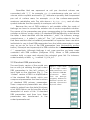
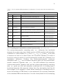
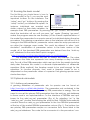
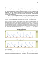
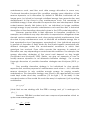
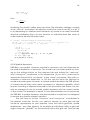
1
DEB-IBM User Manual
Dynamic Energy Budget theory meets individualbased
modelling: a generic and accessible implementation
Benjamin Martin1*, Elke Zimmer2, Volker Grimm1, Tjalling Jager2
Dept. of Ecological Modelling, Helmholtz Center for Environmental Research – UFZ,
Permoserstrasse 15, 04318, Leipzig, Germany
2 Dept. of Theoretical Biology, Vrije Universiteit, de Boelelaan 1085, NL-1081
HV,
Amsterdam, the Netherland
1
This manual explains how to use the model DEB-IBM, which is a NetLogo implementation of a generic individual-based model based on Dynamic Energy
Budget (DEB) theory. It also gives a quick overview of DEB theory and its basic
parameters.
The rationale of the model and its implementation are also explained in:
Martin B, Zimmer E, Grimm V, Jager T. Year. Dynamic Energy Budget
theory meets individual-based modelling: a generic and accessible implementation. Journal Volume: pages.
The NetLogo implementation and the complete model description following
the ODD protocol can be found here:
NetLogo implementation.
ODD model description.
We recommend reading the article and the ODD model description first.
2
Leipzig – Amsterdam December, 2010
*
Corresponding author, email: [email protected]
3
Contents
1. Getting Started ......................................................................................................... 4
1.1 About NetLogo ................................................................................................... 4
1.2 About DEB............................................................................................................ 4
1.3 Installation............................................................................................................ 4
1.4 How to use the model ....................................................................................... 5
2. DEB parameters ........................................................................................................ 6
2.1 DEB notation........................................................................................................ 6
2.2 Standard DEB parameters................................................................................. 7
2.2.1 Feeding and assimilation related parameters: {F&m } , {J& EAm } , yEX ............. 8
2.2.2 Reserve dynamics parameters: κ, v& ........................................................ 9
2.2.3 Somatic growth and maintenance parameters: {J& ET } , [ J& EM ] , yVE ....... 9
2.2.4 Development and reproduction parameters: M Hb , M Hp , k&J , κR .......... 10
2.3 Standard DEB can be expressed in mass or energy ................................... 10
2.4 From standard to compound parameters ................................................... 11
2.5 From standard DEB to scaled DEB ................................................................. 12
2.6 DEB-IBM parameters......................................................................................... 14
3. The interface ........................................................................................................... 14
3.1 Running the basic model ................................................................................ 15
3.2 Optional submodels ......................................................................................... 15
3.2.1 Add my pet parameters........................................................................... 15
3.2.2 Food dynamics........................................................................................... 17
3.2.3 Ageing ......................................................................................................... 17
3.2.4 Stochasticity................................................................................................ 18
3.3 Plots, Histograms and Monitors ....................................................................... 18
4. Procedures ............................................................................................................. 19
4.1 Basic code structure ........................................................................................ 19
4.2. Guide for adapting the model ..................................................................... 20
4.2.1 Feeding ....................................................................................................... 21
4.2.2 Reproduction ............................................................................................. 21
4.2.3 Starvation .................................................................................................... 24
4.2.4 Spatial dynamics........................................................................................ 26
4
1. Getting Started
This manual describes how to install and use the model DEB-IBM, a generic individual-based model that includes general DEB theory as a submodel for the
individuals’ bioenergetics and life-cycle. The main task of users of DEB-IBM will
be to parameterize the model and to possibly revise the underlying NetLogo
program. In this manual we therefore first explain the DEB parameters used in
DEB-IBM and then give examples for how to revise the code. The overall purpose of this model and its implementation are explained in Martin et al.
(Year), whereas the model itself is described using the ODD protocol for describing individual-based models (Grimm et al. 2006, 2010) is available at ODD
website.
1.1 About NetLogo
The model is implemented in NetLogo, version 4.1.1 (Wilensky 1999). NetLogo
is a software platform specifically designed for implementing individual-based
and agent-based models. It includes powerful “primitives” (procedures) that
allow users to implement even relatively complex models with relatively few
lines of code and little or no previous programming experience. Complete
novices to NetLogo and programming can generally program efficiently in 23 days; two textbooks on individual-/agent-based modelling are in press
(Railsback and Grimm, in press1; Wilensky and Rand, in press).
1.2 About DEB
Dynamic Energy Budget theory (DEB theory, Kooijman 2010) provides a set of
rules that specifies the acquisition and use of energy in an organism, and
thereby the life-history traits for the whole life-cycle of a single organism. More
information about DEB can be found on http://www.bio.vu.nl/thb/. By using
the Individual Based Model (IBM) as implemented in NetLogo, it is possible to
investigate the population dynamics of a species, following DEB theory, by inputting the specific metabolic, (DEB) parameters for the species of interest. A
continuously growing library of DEB parameters for all kinds of different species
can be found on the above mentioned homepage, in the DEB laboratory
(see add_my_pet parameter section below ).
1.3 Installation
NetLogo is free software and can be downloaded from:
1
See also www.railsback-grimm-abm-book.com
5
http://ccl.northwestern.edu/netlogo/; versions for the operation systems
Windows, MacOS, and Linux are available. Installation is straightforward and
usually does not take more than five minutes. To run and use the model DEBIBM, start NetLogo and open “DEB-IBM.nlogo” (which comes with the DEB-IBM
package that be downloaded from DEB-IBM webpage.
1.4 How to use the model
NetLogo comes with three tabs: interface, information, and procedures. The
“interface” tab is where users can input the DEB parameters of their species,
alter environmental variables, and observe individual and population level
output of the model. The “procedures” tab contains the NetLogo program, or
code, implementing the DEB-IBM model. Here users can alter model structure,
create new variables to monitor, add procedures for file output, and include
other aspects of importance to the population dynamic of their species such
as behaviour, space, and predation.
There are two levels of use for DEB-IBM. The first requires only familiarity
with the interface. On the interface users can input the DEB parameters of
their species and observe various population and individual variables such as
population density, size structure, and reserve levels under various feeding
conditions (data of all diagrams can be exported via the diagrams’ context
menus or NetLogo’s “export” primitives). This level of use requires no
programming. All information that users need to use the model are the DEB
parameters of their species of interest. Thus, at this level the program allows
users to learn how changes in metabolic parameters alter characteristics of
individual life-histories and population dynamics.
The second level of using DEB-IBM is modifying the generic program to
answer specific research questions or to adapt the model to specific species.
For example, a researcher may be interested in how the population dynamics
of a species is influenced by changes in land use. In this case the researcher
would adapt the standard model to include space and movement behaviour
of individuals, with the DEB theory acting as the energetic model. This more
engaged use of the model requires users to be familiar with both the interface
and procedure tabs. Likewise, species may show specific behaviours that are
not captured by DEB theory; these behaviours could be added to the generic
model. For this second level of using DEB-IBM, basic training in modelling and
NetLogo are required. Beginners in both fields would need obtaining some
literacy in both fields, for example by using the textbook of Railsback and
Grimm (in press).
6
2. DEB parameters
Our implementation of the DEB-IBM is based on the scaled DEB model
(Kooijman et al. 2008) and uses compound parameters. These compound
parameters are derived from the 12 primary parameters of the standard DEB
model. Implementing our model in the scaled version of DEB rather than the
standard DEB model further simplifies the model: by dividing the state
variables “reserve”, “maturity”, and “reproduction” by the maximum surfacearea-specific assimilation rate, one parameter of the standard model is
removed as well as the unit of either energy or mass (standard DEB can be
based in either) from the model. Working with the scaled DEB model with
compound parameters allows parameterizing the DEB model for a species
without directly measuring energy or mass (you cannot estimate energy
parameters without measuring energies). See Kooijman et al. 2008 for a guide
for parameterizing a DEB model.
While the general principles of DEB theory are relatively simple, the
formulas used in our implementation have been algebraically rearranged,
reduced (using compound parameters), and scaled. Thus the resulting
formulas used in DEB-IBM may not seem intuitive. For a novice to DEB theory it
may be difficult to understand what processes are actually driving fluxes for
each of the DEB state variables. To facilitate a better understanding of DEB
theory for those interested in population dynamic applications we below
provide a brief introduction to the standard DEB parameters, how the
compound parameters used in DEB-IBM relate to these parameters, and how
changes in the each of the parameters effects the life-history of the modelled
individuals. In addition to this user manual and the ODD model description,
we
recommend
those
new
to
DEB
theory
to
first
read
(http://www.bio.vu.nl/thb/deb/index.html) for a non-technical introduction to
the concepts of DEB theory and Kooijman et al. (2008) and Kooijman (2010)
for a more formal description. For those already familiar with compound
parameters and the scaled DEB model this section can be skipped.
2.1 DEB notation
In all text (manuscript, ODD model description, and user manual) we used
standard DEB notation. This notation may look somewhat cumbersome at the
beginning, but has a long history and is, by itself, highly consistent. Therefore,
careful attention to the notation will spare users considerable time and
confusion. We recommend routinely using Table 1 in the ODD model
description, which contains a comprehensive list of all parameters dealt with
in both the text and in the implementation of the model.
7
Quantities that are expressed as unit per structural volume are
surrounded with “[ ]”, for example [ J& EM ] is maintenance rate per unit of
volume, while a symbol enclosed in “{ }” indicates a quantity that is expressed
per unit of surface area; for example {J& EAm } is the surface-area-specific
maximum assimilation rate. The dots above J in {J& EAm } , [ J& EM ] , and all other
symbols indicate that the quantity is a rate per unit of time.
Because the use of DEB notation is not possible within the code of
NetLogo we have to convert the notation into a code-compatible notation.
The names of the parameters are given corresponding to the standard DEB
notation as follows: a rate, which is in standard DEB identified by a dot above
the letter, is here identified with the extension “_rate”, For instance, energy
conductance, ν& , is called “v_rate_int”. The “_int” portion refers to the fact
that these are the initial, or baseline, parameters for a species. Users can allow
individuals to vary in their DEB parameters from the initial parameters in some
way, as we do for four of the DEB parameters (see stochasticity section
below). Subscripts and superscripts in DEB notation are indicated by “_” and “
^ ”, respectively. Although NetLogo is not case sensitive we keep cases
consistent with DEB notation (Kooijman 2010). When a DEB parameter
contains both a super and subscript the subscript goes first. For instance,
scaled maturity at birth, U Hb , is written “U_H^b_int”.
2.2 Standard DEB parameters
The most basic version of the model can
be run with just defining the eight scaled
DEB parameters in the left column of
input fields on the interface (Fig. 1). The
“scaled” version of DEB is a simplification
of the standard DEB model, which uses
compound parameters that are functions
of standard DEB primary parameters.
These compound parameters are often
easier to extract from the data (Kooijman
et al. 2008). Below we first provide a brief
description of each of the 12 standard
DEB parameters and then how these
parameters are transformed to the
scaled parameter set.
Figure 1. Input fields
for the eight scaled
DEB parameters used
by default in DEB-IBM
(screenshot
taken
from the NetLogo
program). Differences
between species are
primarily represented
by these values.
8
Table 1. The 12 primary DEB parameters (in dimension of mass) and their associated processes.
Standard DEB Parameters
Symbol Unit
Description
Process
m3d-1m-2
surface-area-specific searching rate
Feeding/assimilation
{J& EAm }
mol d-1m-2
surface-area-specific maximum assimilation
Feeding/assimilation
rate
yEX
mol mol-1
yield of reserve on food
Feeding/assimilation
v&
m d-1
energy conductance
Reserve dynamics
κ
-
allocation fraction
Reserve dynamics
yVE
mol mol-1
yield of structure on reserve
{J& ET }
mol d-1m-2
surface-area-specific somatic maintenance
[ J& EM ]
mol d-1m-3
volume-specific somatic maintenance
M Hb
mol
maturity at birth
M Hp
mol
maturity at puberty
k&J
d-1
specific maturity maintenance
κR
-
reproduction efficiency
{F&m }
2.2.1 Feeding and assimilation related parameters:
somatic
growth/maintenance
somatic
growth/maintenance
somatic
growth/maintenance
reproduction/development
reproduction/development
reproduction/development
reproduction/development
{F&m } , {J& EAm } , yEX
The surface-area-specific searching rate, {F&m } , influences the functional
response for a given prey type. Earlier versions of DEB used the half saturation
coefficient, K, which relates to {F&m } via K = {J& EAm } / [yEX {F&m } ]. Here yEX is the yield
of reserves on food or, in other words, the conversion efficiency of moles of
food into moles of reserve; in most bioenergetic models this is referred to as
assimilation efficiency. Dividing the surface-area-specific maximum
assimilation rate, {J& EAm } , this conversion efficiency gives you the surface-areaspecific maximum ingestion rate, {J& XAm } . The ratio between the maximum
surface-area-specific ingestion rate and the surface-area-specific searching
rate, {F&m } , gives you the half saturation coefficient (K) in a Holling type II
functional response (this response follows from the assumption that the full
time budget of an organism is spent either searching or handling food). In
recent formulations of DEB theory {F&m } has replaced K as a primary parameter
in the standard DEB model because it is more closely linked to the underlying
9
mechanism. For more mechanistic details and reasoning behind the feeding
process see Kooijman (2010, p. 25).
2.2.2 Reserve dynamics parameters: κ, v&
In DEB theory, assimilated energy first enters a reserve before mobilized for
somatic or development and reproduction purposes. One of the assumptions
of DEB theory is “weak homeostasis”, which means that at a constant food
density the ratio of reserves to structure remains constant. The derivation of
reserve dynamics from this assumption is rather complex and explained in
Kooijman (2010, p. 37). In a simplified case of an organism which does not
grow, for reserve density to remain constant assimilation would have to equal
mobilization. However, for growing organisms mobilization must be lower than
assimilation due to dilution of reserve density via growth. The dynamics
resulting from the assumption of weak homeostasis is that mobilization of
reserves will be proportional to reserve density, with the proportionality
constant depending on the ratio of energy conductance, v& , and the length
of the individual. Higher values of energy conductance imply a lower
resistance of transfer from reserves to structure along the reserve-structure
interface, thus the higher the conductance, the faster reserves are depleted
and mobilized for use. The maximum reserve density [EM] is given by the
maximum surface-area-specific assimilation rate, {J& EAm } , and energy
conductance, v& . The allocation fraction parameter, “kappa”, κ, is the
fraction of mobilized reserves which is allocated to somatic growth and
maintenance, while the remainder, (1 – κ), is allocated to development and
reproduction.
2.2.3 Somatic growth and maintenance parameters:
{J& ET } , [ J& EM ] , yVE
The fraction κ of mobilized reserves is allocated to the soma, i.e. the nonreproductive parts of the organism. In the soma, maintenance costs are paid
first and the remaining energy is allocated to growth. There are two basic
categories of maintenance costs, those which are surface-area-specific and
those which are volume-specific. Surface-area-specific costs typically relate
to heat loss of endotherms, but can also represent other surface-area-related
costs such as osmoregulation. In the current implementation of the model we
focus on ectotherms and we assume surface-area-specific costs to be
negligible, i.e. {J& ET } = 0. Volume-specific maintenance rate [ J& EM ] represents the
costs associated with maintaining and implementing somatic functions
(maintaining concentration gradients, turnover of structure, movement).
Because this is a volume-specific rate, volume-related maintenance costs of a
certain individual are obtained by multiplying [ J& EM ] by the individual’s volume,
or structural length cubed, L3 Thus, in the absence of surface-area-related
10
costs, an individual two times larger in volume or weight would have double
the daily maintenance costs. The remaining mobilized energy is converted to
growth, with an efficiency of yVE, or in other words how many moles of
structure are produced from one mol of reserve. Usually, in DEB theory we
consider structure in units of volumetric length, which is L = V1/3 (see Kooijman
2010 p. 10, for explanation structural (volumetric) length in comparison to
measured physical length)..
To convert moles of structure into volume, L 3, or volumetric length, L,
we use [MV] which converts moles to cubic centimetres; a typical value for this
parameter is 4 mmol cm-3 (Kooijman 2010).
2.2.4 Development and reproduction parameters:
M Hb
,
M Hp
,
k&J ,
κR
The fraction of mobilized energy not allocated to the soma, (1–κ), is allocated
to development or reproduction. DEB theory divides the life history of all
species into three classes: embryos, juveniles, and adults. Embryos do not feed
externally but use maternal reserves for growth and development (at
“conception” an embryo is composed of nearly only reserves). A transition
from embryo to juvenile marks a switch to exogenous feeding. Neither
embryos nor juveniles reproduce. The transition from juvenile to adult marks
the start of investment into reproduction (the actual reproduction may occur
a little later). In DEB theory these two transitions are made after a given
amount of mobilized energy, M Hb , has been allocated to maturity to transition
from embryo to juvenile, and M Hp to transition from juvenile to adult. Unlike
structure, maturity has no mass or dimensions but rather is considered
“information” (maturity is quantified by the cumulative amount of reserves
invested in it). Like for soma, individuals must pay costs associated with
maintaining a given level of maturity. These costs are taken proportional to
the maturity level (in mol of invested reserves); the proportionality constant is
the maintenance rate coefficient, k&J , with the units of d-1. Total energy spent
on maintaining maturity is proportional to maturity level. When individuals
reach puberty, at MH = M Hp , maturation is complete and M Hp represents a
maximum value of maturity. Once an individual reaches puberty, energy
remaining after maintenance costs for maturity are paid are allocated into a
reproduction buffer. The reproduction buffer is depleted during reproduction
(the creation of offspring) and is converted into embryonic reserves (embryos
are nearly 100% reserves) with an efficiency equal to κR.
2.3 Standard DEB can be expressed in mass or energy
Seven of the 12 standard DEB parameters shown in Table 1 are expressed in
dimension of mass (mol). However DEB can also be expressed in the
11
dimension of energy (Joules). In this case, different notation is used for those
seven DEB parameters (Table 2).
Table 2. The parameters and units of the energy- or mass-specific parameters in standard
DEB. The five standard parameters not listed are not specific to either energy or mass (Table
1). A typical value to convert between energy and mass is 550 kJ mol-1, and mass can be
converted to volume via [Mv] (Section 2.2.3) with a typical value of 4 mmol cm-3 (Kooijman
2010).
Standard Parameters in mass and energy
Mass (moles)
Symbol
Unit
Energy (Joules)
Symbol
Unit
{J& EAm }
mol d-1m-2
{ p& Am }
yEX
mol mol-1
κX
yVE
mol mol-1
[ EG ]
J m-3
{J& ET }
mol d-1m-2
{ p& T }
J d-1m-2
[ J EM ]
mol d-1m-3
[ p& M ]
J d-1m-3
J d-1m-2
- (assimilation
ciency)
M Hb
mol
E Hb
J
M Hp
mol
E Hp
J
effi-
Table 3. Symbols used for the state variables in the dimensions of mass and energy, and in the
dimensionless scaled DEB used in DEB-IBM.
DEB state variables
State variable
Mass
Energy
Length
L
L
ME
EE
Reserves
Scaled
L
UE
Maturity
MH
EH
UH
reproduction
buffer
MR
ER
UR
2.4 From standard to compound parameters
As mentioned earlier it is often convenient to work with compound
parameters as they require less data to parameterize. These compound
parameters represent combinations of primary parameters that are grouped
together in the differential equations for the standard DEB model. In the
current implementation we used two compound parameters: energy
investment ratio, g, and specific somatic maintenance rate, k&M . The former, g,
is derived from the standard primary parameters using units of mass:
g=
[ M V ] v&
κ {J& EAm } yVE
12
or energy:
g=
[ EG ] v&
.
κ { p& Am }
Because maximum reserve density
[ EM ] =
{ p& Am }
,
v&
we can think of g as the cost to create a unit of structure relative to the
maximum reserve density which would be allocated to the soma:
g=
k&M
[ EG ]
κ [ EM ]
is derived from the standard parameters using units of mass:
[ J& ] y
k&M = EM VE
[M V ]
or energy
[ p& ]
k&M = M
[ EG ]
The reason why we see [ M V ] in the formulas for g and k&M in the mass
parameterization and not in the energy parameterization of the standard DEB
model is that [ EG ] converts energy in reserves to growth in the dimension of
length, while yVE converts moles of reserves to moles of structure and [ M V ] is
needed to convert to structural length.
2.5 From standard DEB to scaled DEB
Using the two compound parameters g and k&M in place of the primary
parameters we get a simplified version of the standard DEB differential
equations for reserves:
(
d
M E = {J& EAm } f L2 − J& EC
dt
)
with
ge ⎛
Lk& ⎞
⎜1 + M ⎟
J& EC = {J& EAm }L2
⎜
g +e⎝
v& ⎟⎠
13
and
e=v
v&M E
L3{J&
EAm }
.
e is the scaled reserve density; the “scaled” is in reference to the amount of
reserves per unit of structure (reserve density) relative to the maximum
amount of reserves per unit of structure. Remembering that maximum reserve
density
[ EM ] =
{J& EAm }
v&
we see that e is the total mass of the reserves divided by volume and
maximum reserve density and will have a value between 0 and 1. The
changes in DEB’s three state variables (Table 3), length, maturity, and
reproduction buffer can then be calculated as follows:
(
)
⎛ κJ& − [ J& EM ]L3 yVE
d
L = ⎜⎜ EC
[MV ]
dt
⎝
⎞
⎟
⎟
⎠
1
3
d
M H = ((1 − κ ) J& EC − k&J M H ) for M H < M Hp else d M H = 0
dt
dt
d
d
M R = ((1 − κ ) J& EC − k&J M Hp ) for M H > M Hp else
MR = 0 .
dt
dt
As we mentioned earlier our model is implemented in the scaled version of
DEB. By this we mean that to remove the unit mol (or Joule if using the energy
parameterization of DEB) we divide all state variables in moles (ME, MH, and
MR) by the maximum surface-area-specific assimilation rate {J& EAm } (or { p& Am } if
working with energy) to get scaled reserve UE , scaled maturity UH, and scaled
reproduction buffer UR (Table 3). Dividing both sides of the three differential
equations by {J& EAm } gives:
d
U E = ( fL2 − SC )
dt
With SC = L2
ge ⎛ Lk&M ⎞
⎟
⎜1 +
g + e ⎜⎝
v& ⎟⎠
d
U H = ((1 − κ ) SC − k&J U H ) for U H < U Hp else d U H = 0
dt
dt
d
d
U R = ((1 − κ ) SC − k&J U Hp ) for U H > U Hp else U R = 0 .
dt
dt
14
Notice that we now use scaled U Hp and U Hb for parameters related to lifestage transitions, which are equal to M Hp and M Hp divided by {J& EAm } .
The length dynamics simplify to:
d
L=
dt
⎞
1 ⎛ v&
⎜⎜
SC − k&M L ⎟⎟ .
2
3 ⎝ gL
⎠
2.6 DEB-IBM parameters
We have now derived the equations used in DEB-IBM. If food conditions are
Figure 2. The interface of DEB-IBM. Elements of the Interface are buttons (e.g., setup), input fields (e.g., E_H_b), sliders (e.g., timestep), choosers (e.g., aging), monitors (e.g., count
turtles), and plots (e.g., population density).
constant we only need eight parameters to run simulations. To run DEB-IBM at
constant food conditions, set the “food-dynamics” chooser to “constant” and
set scaled assimilation rate to the desired value. The input boxes for the eight
parameters needed to run DEB-IBM at constant food conditions are on the
left-most side of the interface (Fig. 1). The bottom four parameters in the column are primary DEB parameters ( v& ,κ, κ R, and k&J ). The top four parameters
include the two compound parameters g and k&M , in addition to the two lifestage transition parameters, U Hb and U Hp .
3. The interface
In Fig. 2, you see how the interface looks like after opening the model in NetLogo.
15
3.1 Running the basic model
The first thing you should know is how to
run the model. In Fig. 3, you see the most
important buttons on the interface: The
“setup” and “go” buttons. By pressing the
“setup” button, you initialize the system, for
instance, individuals are created and Figure 3. These buttons are needed
to run the model
obtain values for their state variables, for
example their DEB parameters. By pressing the “go“ button, the simulation
starts; the simulation will run until you press “go” again. (Pressing “go-once”
makes the program execute one timestep.) In the current implementation of
the model the parameters for a species are set for individuals during the setup
procedure. Thus altering a parameter value in the interface will not result in a
change in the DEB individuals’ parameter values unless the setup procedure is
run after the changes were made. This could be altered to allow “midsimulation” modification of parameter values. In the basic version of the
model, all of the standard DEB parameters are derived from the “Add my
pet” database for the water flea Daphnia magna,
(http://www.bio.vu.nl/thb/deb/deblab/add_my_pet/index.php).
The timestep slider allows the user to control the timestep. The value
selected on the slider bar represents how many timesteps a day is divided
into. Thus all of the DEB parameters which are input into the model should be
daily rates. Because the model is a discrete implementation of differential
equations (Euler method), the timestep needs to be small enough for the
equations to function properly. How small a timestep needs to be is
dependent on the parameter values of a species. Fast-growing species need
shorter time steps.
3.2 Optional submodels
3.2.1 Add my pet parameters
A growing database of parameter sets for species can be found at:
http://www.bio.vu.nl/thb/deb/deblab. The parameter sets contained in the
“add my pet” database are the primary DEB parameters in energy. Thus we
need to convert the primary DEB parameters from the add_my_pet database
to those used in our implementation. On the interface of DEB-IBM are input
boxes for five add_my_pet parameters (Fig. 4). By selecting “on” in the
“add_my_pet” chooser and clicking the setup button, DEB-IBM automatically
converts these five add_my_pet parameters to the four DEB-IBM parameters
at the top of the scaled DEB-IBM parameters column (Fig. 1). The bottom four
are primary DEB parameters require no conversion from those listed in the
add_my pet database. The code for the conversion is in the procedure “con-
16
vert-parameters” within the “setup” procedure. In the following paragraph,
we explain how these parameters are calculated.
Noticeably
missing
from
the
Figure 4. The four top
add_my_ pet database is the maximum
parameters in Fig 1.
surface-area-specific
assimilation can be calculated
parameter, { p Am } . This is because { p Am } is from these five pafood type specific. Some food types are
of higher energetic value than others
and thus organisms raised on ad-libidum
concentrations of varying quality food
can assimilate, and thus grow at different
rates. However, we can use the “zoom”
factor to estimate the value of { p Am } . The
rameters given in the
“add my pet” database.
zoom factor is the maximum volumetric
length, LM, of an organism in centimetres.
It is called the zoom factor because DEB
theory makes several predictions for scaling of DEB parameters interspecifically with body size, and the scaling of these parameters leads to many
observable covariations such as growth rate, respiration, and life span (van
der Meer 2006; Kooijman 2010, chapter 8). In DEB theory maximum length is a
function of three primary parameters: maximum assimilation rate, kappa, and
volume-specific maintenance costs.
LM = κ
{ p& Am }
.
[ p& M ]
Because add_my_pet gives values for all the parameters in this equation
other than { p Am } , we can rearrange the formula to determine its value. Once
the value of { p Am } is determined, all other conversions are straightforward.
For U Hb and U Hp , we need to convert maturation threshold for birth and
puberty to scaled maturity at birth and puberty by dividing by the surfacearea-specific maximum assimilation rate:
U Hb = E Hb /{ p Am } And U Hp = E Hp /{ p Am } where { p Am } =
[ p& M ]z
κ
For the two compound parameters we just use the formulas consisting of primary DEB parameters:
[ p& ]
k&M = M and
[ EG ]
g=
[ EG ]v&
{ p& Am }κ
17
3.2.2 Food dynamics
In the basic version of the model, the Figure 5. Feedscaled functional response, f , (f_scaled ing- related pain DEB-IBM) is set to 1 (ad-libidum feeding rameters as seen
conditions). Keeping the food-dynamics on the interface.
constant, you can change the food In the “fooddynamics”
supply by changing f_scaled on the chooser, “conslider. This can be done while the model stant” or “logisis running without a new setup.
tic” can be seIf you want to simulate a scenario l t d
with a dynamic food source, you can change the food-dynamics to “logistic”
(just click on it). In the built-in scenario, a logistically growing prey population is
depleted by the DEB population via predation. This is a very simple scenario,
and it may be more realistic to let the DEB animal feed on another DEB organisms but this is too specific for this implementation. For “logistic” prey dynamics, two new parameters are needed for the DEB individuals {J& XAm } and {FM } .
{FM } is a primary DEB state variable for maximum surface-area-specific search
rate and {J& XAm } is maximum surface-area-specific ingestion rate. {J& XAm } differs
from
{J& EAm }
in that the latter only considers assimilated energy or
{J& EAm } = {J& XAm } yEX .
The prey population is characterized by the state variable density, X,
and two parameters describing population growth rate, r, and carrying capacity K , respectively. For details see the prey dynamics submodel in the
ODD model description. In the default model we assume feeding takes place
in a three-dimensional environment (e.g. aquatic filter-feeders). However this
can be modified to model feeding over two-dimensional surfaces. The parameter “volume” represents the size of the environment. The feeding submodel is only connected to the standard DEB model via the dimensionless
scaled assimilation rate, f. Therefore, the units of X and volume can be userdefined (e.g. energy liter-1, mg cm-3, cells per mm-3) as long as they are consistent with each other.
3.2.3 Ageing
In the basic version of the model, the
ageing submodel is turned “on”.
Individual’s age as described in
Kooijman (2010) and the ageing submodel section of the ODD. If the ageing
submodel is turned off, animals have a
daily background mortality rate.
Figure
6.
Parameters as seen
on the interface
which affect the
ageing
submodel.
18
3.2.4 Stochasticity
In the standard DEB model the only Figure 7. parameter
which controls the
inherent
coefficient of variasource of stochasticity comes from the
tion. If set to 0, there
ageing
is no intraspecific
submodel. This can lead to extreme variation in DEB papopulation
fluctuations because life-histories are exactly
the same for all individuals which leads to synchronisation. One likely reason
natural systems do not always exhibit such drastic fluctuations is that stochastic processes and heterogeneity among individuals prevent strong synchronization of life histories. One way of incorporating stochasticity is to allow individuals to vary in some of their DEB parameters. This method is justified because experiments often find that repeated physiological measurements of
individuals are less variable then those between individuals.
We followed the method outlined in Kooijman (1989) where individuals
have a random component in the maximum surface-area-specific ingestion
rate, {J& EAm } . In our implementation of the scaled DEB model there is no
parameter {J& EAm } because we scaled it out of our model, but changing {J& EAm }
affects other parameter values indirectly. Both values of the life-stage
transition parameters will be affected because they are both scaled by {J& EAm } .
The maximum surface-area-specific ingestion rate will be influenced
{J& XAm } = {J& EAm } /yEV , which further influences the half-saturation coefficient K as K
= {J& EAm } / [yEX {F&m } ], and finally it affects g as {J& EAm } is in the denominator of this
formulation.
Thus, variation in all of these parameters is included by multiplying (for
&
{J XAm } ) or dividing (for g, U Hb , and U Hp ) by a “scatter-multiplier” which is a lognormally distributed number with user-defined standard deviation “cv”. Users
can select the value of cv in the “cv” input box. Entering a value of 0 results in
all individuals having the same parameters.
Obviously there are many other sources of stochasticity in natural
systems. However the sources of stochasticity to be included in the model are
likely to be system-specific and should be carefully considered by the
researcher.
3.3 Plots, Histograms and Monitors
In the default model we include several output plots and histograms to
monitor the population dynamics of the modelled species. A plot of the
population density, a plot of their prey density, and a plot of the stage class
density with the x axis in days (embryo, juvenile, and adult). Additionally there
are three histograms, i.e. the frequency distribution of length, L, and scaled
19
reserve density, e, for both juveniles and adults. Ultimately the user can record
and plot any individual- or population-level variable of interest. For
information on generating output data, plots, monitors, and histograms, see
the NetLogo User manual and programming guide.
Figure 8. The three default plots and three histograms displayed on the DEB-IBM interface. The
plot “stage class density” shows the density of each life stage (embryo, juvenile, and adult)
over time. The plots “food density” and “population density” show the density of the food (X)
and total population. The “size distribution” histogram shows the distribution of lengths (L) of
the population. The histograms “juv e distribution” and “adult e distribution” give the distribution of scaled reserve density (e) of juveniles and adults.
4. Procedures
In this tab the structure of the model can be modified and other aspects
relevant to population dynamics can be included. Here we discuss the basic
structure of the code and suggest how to modify it.
4.1 Basic code structure
The first section of the code declares the variables and specifies which type of
variables they are. DEB individuals are referred to as “turtles", which is the
NetLogo term for “agent” or “individual”. Turtle variables are state variables
characterizing the state of a certain turtle, i.e. L, UE and UH. Additionally,
20
because we allow some of the DEB parameters to differ between individuals,
we made the entire set of DEB parameters turtle variables (Grimm et al. 2010).
In NetLogo, the spatial arena consists of square grid cells, called
patches. The default model is non-spatial and therefore consists of only one
patch (updating the view of the model world, or “view”, is therefore
deactivated in the program). Patch variables are the state variables of a
patch. In our model the density of prey is a patch variable. This allows to easily
make the model spatially explicit by defining a grid of patches, each with
their own states, e.g. prey and turtle density. Local predator-prey interactions
are then easy to include, e.g. feeding of DEB predators on a patch only
reduces the prey density on that patch.
Finally, global variables are typically parameters which can be used by
either turtles or patches. Globals can either be declared in the procedures
tab or created on the interface tab, in which case they are not declared in
the “globals-own[]”.The DEB parameters which do not vary between
individuals could have been made global variables but we chose to make
them turtle variables so that users could allow individuals to vary in any DEB
parameter with little programming effort. Note that on the interface, you can
only use global variables, no turtle or patch variables. Therefore, all eight DEB
parameters on the interface (Fig. 1) are distinguished from the turtles variables
by the suffix “_int”; four of these parameters are then made to vary between
individuals (see section 3.2.4).
The remainder of the code includes two major procedures: setup and
go. The setup procedure involves all processes required to initialize the model.
In the setup procedure some initial individuals are created and their state
variables and parameters are specified. A detailed description of the
initialization is given in the ODD model description. The go procedure runs the
population model. An overview of the model processes and their scheduling
and a detailed description of each submodel are given in the ODD model
description.
4.2. Guide for adapting the model
For most applications the default model will need to be adapted in some way
to address a specific research question. These alterations may be either to
adapt the standard DEB model to reflect the life-history of the species of interest (ex. modifying the reproduction submodel) or adapt the model to address a specific research question (ex. Including spatial dynamics or more
complex prey dynamics). Below we provide some examples of how the default model can be adapted. In each example we show the major code
changes needed to implement each model adaptation, however the complete code for each example is given on the website.
21
4.2.1 Feeding
In the standard DEB model, the assimilation rate depends on the surface area
of the predator and the density of the prey. These two variables are often
sufficient to describe feeding rates in controlled laboratory settings. Usually,
however, varying environmental conditions strongly influence foraging
success. For example light intensity, turbidity, and turbulence strongly
influences encounter rate and capture success for most visual predators in
aquatic environments. Different types of habitat provide varying degrees of
refuge for prey species thus influencing the foraging rate of predators. These
influences can be easily incorporated into DEB-IBM via a mechanistic foraging
submodel or a simple modification of f as a function of important
environmental variables.
4.2.2 Reproduction
Differences between species are for the most part characterized by
differences in their set of DEB parameters. However, species also exhibit
differences in behaviour which are important for population dynamics. In the
context of the DEB model, the most notable variation in behaviour is the
reproduction strategy of a species. The default reproduction strategy in the
model is for mature individuals to check if they have enough energy to
reproduce; if they do they produce one embryo. Altering the reproductive
strategy of the DEB individual to produce clutches of offspring requires a
minor modification of the code. Below we give an example of how to modify
the reproduction behaviour of the DEB animal.
DEB theory assumes that mothers in good conditions (higher scaled
reserve density) produce higher quality offspring (offspring with higher scaled
reserve density). This has been observed for many species, but there are
exceptions (Kooijman 2010). Thus in the standard DEB model, mothers invest
enough energy in an embryo so that when the embryo hatches (U_H = U_H_B)
its scaled reserve density will be equal to its mothers scaled energy density. In
the default version of DEB-IBM, mature individuals reproduce when they have
enough energy to produce a single embryo with enough reserves to meet the
condition noted above.
However, the water flea Daphnia magna does not produce one
offspring at a time, but rather mature daphnids produce new broods every 23 days and the release of a brood coincides with molting. Time between
reproduction events for Daphnia is dependent on temperature, but is
independent of food. Because we are considering a situation where
temperature is constant, we will assume that some internal clock triggers
molting, and subsequently reproduction, at fixed intervals. To accomplish this,
we need to give Daphnia individuals a new state variable (“repro-time”) to
keep track of time since the last reproduction event, which increases by 1
22
each timestep (remember “timestep” represents how many timesteps one
day is broken up into). We also need to create a global variable “daysbetween-repro”, which is a parameter representing how many days are
between reproductive events; we will set this value to 2.5 days.
We update the reproduction part of the “go” procedure as follows:
[
if U_H >= U_H^p
[
set repro-time repro-time + (1 / timestep)
if repro-time > days-between-repro
[
calc-lay-eggs
if lay-egg? = 1
[
calc-embryo-reserve-investment
lay-eggs
]
]
]
]
As we see above, individuals only reproduce when their time since last
reproduction is greater than the new parameter “days-between-repro” which
represents the time between reproduction events. “Calc-lay-eggs” is the next
procedure which makes sure the individual has enough energy in the repro
buffer to create at least one embryo. If not, repro-time will be set back to 0,
and the reproduction buffer remains unchanged. The individual will then
continue to accumulate energy in the reproduction buffer for another 2.5
days and then reproduce.
to calc-lay-eggs
set L_embryo L_0
set U_E_embryo U_R * kap_R
set U_H_embryo 0
loop [
…
if U_H_embryo > U_H^b * 1 [ set lay-egg? 1 stop]
if e_scaled_embryo < e_scaled [set repro-time 0 stop]
]
end
Once the energy required to create one offspring is determined, the
individual will produce as many offspring as it has reserves for, each with the
initial reserves equivalent to the value determined using the bisection method
in
the
“calc-embryo-reserve-investment”
procedure
(see
http://en.wikipedia.org/wiki/Bisection_method ). The bisection method
determines initial reserves via adaptive trial and error. Each estimation is the
mean (therefore the name of this method, “bisection”) of upper and lower
bounds set for the possible values of “initial reserves”. In the first estimation the
23
upper bound is U_R / kap_R (this is because this is the highest value a mother
can invest in an offspring), and a lower bound of 0. A simulation of the
embryonic life stage is then run, and if the embryo matures with too much
energy remaining in its reserves when it reaches energy for birth, the upper
bound is then set to the previous “estimation”. We can do this because we
know if the estimation was too large then all values larger than estimation will
be too large and thus we can exclude those values from the range of
possible values. If the value set for initial energy results in to little reserves left
when the embryo reaches maturity needed to hatch, or the embryo has to
little energy to reach the maturity threshold for hatching, the lower bound is
then set to the “estimation” of initial reserves used in the simulation. This
process repeats itself until the reserve density of the embryo’s matches that of
the mothers within some acceptable range of error. In this simulation we allow
5% deviation between the embryo’s and mother’s reserve density.
to lay-eggs
hatch floor (U_R / estimation)
[
set die? 0
set mother-id id
set id who
set scatter-multiplier e ^ (random-normal 0 cv)
…
]
set lay-egg? 0
set repro-time 0
set U_R U_R - floor (U_R / estimation) * estimation
end
Notice that we also created two new state variables, “mother-id” and “id”.
This section of code sets the mother-id of a new turtle to the id of the mother
and the id of the new turtle to “who”: a built-in state variable of each turtle
which is a unique identity number. We create these state variables because
Daphnia carry their broods internally; thus if the mother dies, so do her
offspring. We then have to modify the “update” procedure so that when a
mother dies, the program checks to see if she is carrying any embryos (if she
is, they die too).
to update
; individuals update their state variables based on the calc_state variable
; proccesses
ask turtles
[
…
if die? = 1 and U_H >= U_H^p
[
let m-id id
let offspring turtles with [mother-id = m-id and U_H < U_H^b]
if any? offspring [ask offspring [die] ]
die ; the mother then dies
]
24
if die? = 1 [die] ;
]
…
end
An important thing to remember is that all new state variables must be
declared, either as “turtles-own” of global variables. Here, all variables except
for “days-between-repro” (which is a global variable that we declared in the
interface) are turtle variables. Additionally, in the setup procedure you have
to tell turtles to “set id who” within the brackets following the hatch primitive
where turtles are created.
Below we show comparisons of the population dynamics under logistic
prey dynamics, where on the top frame the population uses the Daphnia reproduction behaviour and the bottom frame is the default reproduction behaviour. Daphnia parameters were taken from the add_my_pet database.
Figure 9. Density of 3 life-stages: embryo (black), juvenile (blue), and adult (red), under the
default reproduction strategy (reproduce when enough energy to create one embryo), and
the daphnia reproduction strategy (release broods at fixed intervals, 2.5 days). In the default
strategy eggs are laid externally and survival is not dependant on the mother’s survival, in the
daphnia reproductive strategy if the mother dies while carrying embryos, those embryos also
die. The predation submodel parameters of: {J& } = 1, F = 1, X = 0.5, X = 2, and volume =
XAm
m
r
k
5. Below we see that the two reproduction strategies overall do not result in widely different
population dynamics.
Default reproduction
“Daphnia” reproduction
4.2.3 Starvation
Starved individuals follow standard reserves dynamics until their scaled
reserves, e, falls below their scaled length L / Lm. Under this condition,
individuals no longer mobilize enough reserve to the soma to pay somatic
25
maintenance costs, and thus must alter energy allocation in some way.
Continued starvation beyond this condition requires some alteration of the
reserve dynamics or its allocation. By default in DEB-IBM, individuals will no
longer grow, but divert just enough mobilized energy from reproduction and
development to the soma to pay maintenance costs. The remainder of
mobilized energy is then allocated to reproduction and development. When
scaled reserve density falls below κL/Lm, an individual no longer mobilizes
enough energy to pay somatic maintenance costs and thus dies. A technical
description of the starvation submodel is given in the ODD model description.
However, species differ in their response to starvation conditions. For
example, an individual may stop allocation to reproduction altogether when
starved, reduce maintenance costs, stop paying maturity maintenance, burn
structure to pay maintenance costs, or allocate all available energy into a
final reproduction bout (emergency reproduction). How individuals respond
to periods of starvation is likely driven by the fitness benefits associated with
different strategies under the environmental conditions in which their
genotype has evolved. Even within species the response to periods of
starvation can vary depending on environmental conditions. For example, the
energy allocation strategies of the pond snail depend on day length
(Zonneveld and Kooijman 1989). Below, we give an example of how to
modify reserve dynamics to an alternate starvation strategy. For a more
thorough discussion of possible starvation strategies see Kooijman (2010, p.
118).
One possible starvation strategy is for individuals to stop growth,
reproduction, and the payment of maintenance costs when e < L/LM and alter
reserve dynamics to only mobilize enough energy for paying somatic
maintenance. This starvation strategy was found to be appropriate for pond
snails kept under short day conditions (12 hrs light / 12 hrs dark). In the
unscaled version of the model this would be easy to implement, just by setting
mobilization:
p& C = [ p& M ]L3
(Note that we are dealing with the DEB in energy and p& C is analogous to
{J& } .)
EC
However, DEB-IBM is scaled and uses compound parameters which require some rearrangement.
SC =
and
p& C
[ p& ]L3
= M
{ p& Am } { p& Am }
26
[ EG ] = gκ { p& Am } v&
thus:
SC =
k&M gκ 3
L .
v&
Modifying the model is rather easy from here. The starvation strategy is coded
in the “calc-dL” procedure. We need to modify the code to set dU_H or dU_R
to 0 (depending on whether and individual is a juvenile or an adult) and then
alter the mobilization flux to its new formula. An individual then dies when its
scaled reserve density falls below zero.
to calc-dL ; calculate change in structural length
set dL
((1 / 3) * (((V_rate /( g * L ^ 2 )) * S_C) - k_M_rate * L))
if e_scaled < L / (V_rate / ( g * K_M_rate))
[
set dl 0
ifelse U_H < U_P_H
[set dU_H 0]
[ set dU_R 0]
set S_C (k_M_rate * kap * g * L ^ 3) / v_rate
set dU_E S_A – S_C
if e_scaled =< 0 [die]
]
end
4.2.4 Spatial dynamics
DEB-IBM is non-spatial. However population dynamics can be influenced by
the spatial distribution of resources. The model can be made spatial by clicking on the settings button on the interface tab and setting the “max-xcor”
and “max-pycor” coordinates to the desired size. (If you do so, make sure to
deactivate the primitive “no-display” in the “setup” procedure.) Files with coordinates of resource distribution, or GIS files can be input into NetLogo to
model real landscapes. However, to include spatial dynamics the DEB species
of interest should likely have some movement or dispersal capability which
requires including a dispersal submodel in the procedure tab. Below we present an example of how to include spatial dynamics into the current version
of the model. This example is meant to only demonstrate how to technically
link DEB-IBM to spatial dynamics; the demonstration model was not designed
to answer any specific research question.
First you have to set the “max-xcor” and “max-pycor” coordinates to
the desired world size. For this, you need to decide on what grid cell size
would be appropriate for your question. Note that within grid-cells, spatial
relationships are often ignored, for example all individuals within a grid cell
might compete “globally” for the resources within the grid cell. Grid cell size
27
usually is chosen to represent typical distances of local competition (for
further aspects of choosing appropriate spatial and temporal scales, see
Grimm and Railsback, 2005, and Railsback and Grimm [in press]).
We arbitrarily picked a 80 by 80 grid. We then included a submodel in
the “go” procedure after all the DEB procedures. We implemented a
simplified version of the movement heuristic used in Hancock (2006). Once
every day the individuals make a probabilistic decision whether to stay in their
current patch or move to one of their eight neighbouring patches, where the
probability of staying on its current patch or moving to a neighbour patch is
proportional to the relative amount of resources in each patch. To
accomplish this, at the first time step of every day the food (x) on the eight
neighbouring patches and in the turtle’s current patch are summed. The
probability of the individual of moving to (or staying on) patch i of the nine
patches is determined by:
Pr( Pi ) =
xi
9
∑ xj
j
Below we show the entire movement submodel procedure. This procedure is
run for each individual. We use “p-“ to denote “probability”, followed by the
coordinates of the patch of interest relative to the patch the turtle currently
occupies: a (above), b (below), r (right), and l (left), and h (here, patch the
individual is on). Combinations of two letters denote the patches located
diagonally from the current patch, e.g. “p-ar” is the patch above and to the
right. Then, we choose the target patch by drawing a uniformly distributed
random number from the interval [0, 1] and assigning target patches
according to intervals within [0, 1] that correspond to the target patches
probability of being chosen, i.e. Pr( Pi ) .
to movement-submodel
ask turtles with [U_H > U_H^B] [if ticks mod timestep = 0
[
let scale sum [x] of neighbors + [x] of patch-here
let p-a [x] of patch-at 0 1 / scale
let p-b [x] of patch-at 0 -1 / scale
let p-r [x] of patch-at 1 0 / scale
let p-l [x] of patch-at -1 0 / scale
let p-ar [x] of patch-at 1 1 / scale
let p-br [x] of patch-at 1 -1 / scale
let p-al [x] of patch-at -1 1 / scale
let p-bl [x] of patch-at -1 -1 / scale
let p-h [x] of patch-at 0 0 / scale
let random-number random-float 1
if random-number < p-a
[move-to patch-at 0 1]
if random-number >= p-a and
28
if
if
if
if
if
if
if
random-number < p-a + p-b
[move-to patch-at 0 -1]
random-number >= p-a + p-b
and random-number < p-a + p-b + p-r
[move-to patch-at 1 0]
random-number >= p-a + p-b + p-r
and random-number < p-a + p-b + p-r + p-r
[move-to patch-at -1 0]
random-number >= p-a + p-b + p-r + p-l
and random-number < p-a + p-b + p-r + p-l + p-ar
[move-to patch-at 1 1]
random-number >= p-a + p-b + p-r + p-l + p-ar
and random-number < p-a + p-b + p-r + p-l + p-ar + p-br
[move-to patch-at 1 -1]
random-number >= p-a + p-b + p-r + p-l + p-ar + p-br
and random-number < p-a + p-b + p-r + p-l + p-ar + p-br + p-al
[move-to patch-at -1 1]
random-number >= p-a + p-b + p-r + p-l + p-ar + p-br + p-al
and random-number
< p-a + p-b + p-r + p-l + p-ar + p-br + p-al + p-bl
[move-to patch-at -1 -1]
random-number >= p-a + p-b + p-r + p-l + p-ar + p-br + p-al + p-bl
[move-to patch-at 0 0]
]
Additionally to show the spatial distribution of prey density we can implement
the following code in the go statement following the movement-submodel
procedure.
ask patches ask patches [ set pcolor scale-color green X 2 0]
This line of modified code does not affect the model run but scales the color
of each patch to its level of food density (see primitive “scale-color” in color
subsection of NetLogo programming guide). Because food density is a patch
state variable, each patch has an independent food density which
undergoes logistic growth. Predation is local, as DEB predators only reduce
the density of prey in the patch they currently occupy.
29
Figure 10. Results of a simulation in an 80 x 80 patch environment. Parameters were taken
from the add_my_pet database for Daphnia magna. Food submodel parameters were
set to: submodel parameters of: {J& } = 1, F = 1, X = 0.5, X = 2, and volume = 0.01 . The
XAm
m
r
k
simulation was run for 180 days. The three panels on the left show stage class density,
mean food density of the patches, and population density. The “view” of the simulated
arena on the right shows the spatial distribution of resources at day 230 of the simulation.
Notice that in Fig. 10 the population initially shows large fluctuations but eventually, these fluctuations dampen dramatically. It is interesting to note that
here population oscillations are much smaller than in the non-spatial model.
Like many other models DEB population models typically exhibit the phenomenon known as “paradox of enrichment”. When carrying capacity of the
food is much higher than the half-saturation coefficient, which in our feeding
model is given by: {J& XAm } / Fm , the population will often show large fluctuations,
and if the carrying capacity of the food is much higher the populations will
even collapse. The above example shows how the inclusion of spatial dynamics and the movement behaviour of individuals can lead to a resolution of the
paradox of enrichment. However this is just one mechanism which can stabilize populations, but many other processes can also stabilize populations at
high food carrying capacities such as: inducible defences of the prey type,
multiple prey types, interference competition, environmental heterogeneity
and stochasticity. The importance of these mechanisms should be considered
when modelling in a population context, and the inclusion of one or more of
these mechanisms may be required to replicate realistic population dynamics.
30
References
Grimm V, Berger U, Bastiansen F, Eliassen S, Ginot V, Giske J, Goss-Custard J,
Grand T, Heinz S, Huse G, Huth A, Jepsen JU, Jørgensen C, Mooij WM, Müller B,
Pe'er G, Piou C, Railsback SF, Robbins AM, Robbins MM, Rossmanith E, Rüger
N, Strand E, Souissi S, Stillman RA, Vabø R, Visser U, DeAngelis DL. (2006) A
standard protocol for describing individual-based and agent-based models.
Ecological Modelling, 198,115-126.
Grimm V, Berger U, DeAngelis DL, Polhill G, Giske J, Railsback SF. (2010) The
ODD protocol: a review and first update. Ecological Modelling, 221, 27602768.
Hancock, P. A., and E. J. Milner-Gulland. (2006) Optimal movement strategies
for social foragers in unpredictable environments. Ecology, 87, 2094–2102.
Kooijman, S. A. L. M., T. Sousa, L. Pecquerie, J. Van der Meer and T. Jager.
(2008) From food-dependent statistics to metabolic parameters, a practical
guide to the use of Dynamic Energy Budget theory. Biological Reviews, 83,
533-552.
Kooijman, S. A. L. M. (2010) Dynamic Energy Budget theory for metabolic organisation. Cambridge University Press.
Van der Meer, J. (2006) Metabolic theories in ecology. Trends in Ecology and
Evolution, 21, 136-140.
Zonneveld C. and S. A. L. M. Kooijman. (1989) Application of a general energy
budget model to Lymnaea stagnalis. Functional Ecology, 3, 269-278.