1
HMGC User guide
Last update: June 13, 2008
G. Vlad, S. Briguglio, G. Fogaccia, C. Di Troia
Associazione Euratom-ENEA sulla Fusione, C.R. Frascati,
C.P. 65 - I-00044 - Frascati, Rome, Italy
Manuale utente di HMGC
G. Vlad, S. Briguglio, G. Fogaccia, C. Di Troia
Riassunto
Questo manuale descrive l’utilizzo di HMGC (Hybrid MHD Gyrokinetic Code), il codice di simulazione
3-D ibrido magnetoidrodinamico-girocinetico a particelle, sviluppato a Frascati nei primi anni ’90.
HMGC `e stato sviluppato per studiare l’interazione nonlineare di ioni energetici con turbolenza di tipo
Alfv´enico, in plasmi che bruciano. Il modello di plasma adottato nel codice HMGC consiste in una
componente di plasma termico (core) e una popolazione di ioni energetici. La prima `e descritta dalle
equazioni della Magneto-idro-dinamica (MHD) ridotte O(3 ) nel limite di pressione nulla (dove `e
l’inverso del rapporto di aspetto del toro), inclusi termini resistivi e viscosi. La popolazione di ioni
energetici `e descritta dall’equazione di Vlasov girocinetica nonlineare, espansa nel limite k⊥ ρH 1
(k⊥ essendo la componente perpendicolare al campo magnetico del vettore d’onda, e ρH il raggio di
Larmor degli ioni energetici), con gli effetti di orbita di deriva magnetica pienamente ritenuti, e risolta
con tecniche particle-in-cell (PIC). Lo scopo di questo manuale utente `e quello di rendere il lettore in
grado di utilizzare il codice e di analizzarne i risultati con un insieme di strumenti grafici, anch’essi
descritti con un certo dettaglio.
Parole chiave: Prodotti di fusione, Particelle alfa, particelle veloci, Magnetoidrodinamica (MHD),
Onde di Alfv´en, Tokamaks, Tecniche Particle-in-cell (PIC), Simulazioni girocinetiche
HMGC user manual
Abstract
This user guide describes the use of HMGC (Hybrid MHD Gyrokinetic Code), the hybrid MHD-particle
3-D simulation code developed in Frascati in the early 90s. HMGC has been written in order to study
nonlinear interactions of energetic ions with the Alfv´enic turbulence in burning plasma conditions. The
plasma model adopted in the HMGC code consists of a thermal (core) plasma and an energetic-ion
population. The former is described by reduced O(3 ) Magneto-Hydro-Dynamics (MHD) equations in
the limit of zero pressure ( being the inverse aspect ratio of the torus), including resistivity and viscosity
terms. The energetic-ion population is described by the nonlinear gyrokinetic Vlasov equation, expanded
in the limit k⊥ ρH 1 (with k⊥ being the perpendicular component of the wave vector to the magnetic
field, and ρH the energetic-ion Larmor radius), though fully retaining magnetic drift orbit widths, and
solved by particle-in-cell (PIC) techniques. The aim of this user guide is to make the reader able to run
the code and analyze its results using a suite of graphics tools, also described in some detail.
Keywords: Fusion products, Alpha particles, Fast particles, Magnetohydrodynamic (MHD), Alfv´en
waves, Tokamaks, Particle-in-cell (PIC) techniques, Gyrokinetic simulations
Contents
1 Introduction
7
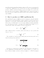
2 How to produce an MHD equilibrium file
9
3 Execution script
15
3.1
Include file modi inc . . . . . . . . . . . . . . . . . . . . . . . . . . . . .
16
3.2
Input file PARAM . . . . . . . . . . . . . . . . . . . . . . . . . . . . . . . .
17
3.3
Input file stop run . . . . . . . . . . . . . . . . . . . . . . . . . . . . . .
21
3.4
Input file TMODE . . . . . . . . . . . . . . . . . . . . . . . . . . . . . . . .
22
3.5
Input file TMODE PL . . . . . . . . . . . . . . . . . . . . . . . . . . . . . .
23
3.6
Include file grid inc . . . . . . . . . . . . . . . . . . . . . . . . . . . . .
24
3.7
Input file KININP . . . . . . . . . . . . . . . . . . . . . . . . . . . . . . .
26
3.8
Input files: energetic particle density and temperature profiles . . . . . .
30
4 Output files: produced by the MHD module
31
4.1
Output file CTTO . . . . . . . . . . . . . . . . . . . . . . . . . . . . . . .
31
4.2
Output file ENERGY . . . . . . . . . . . . . . . . . . . . . . . . . . . . . .
31
4.3
Output file CTBO . . . . . . . . . . . . . . . . . . . . . . . . . . . . . . .
37
5 Output files: produced by the gyrokinetic module
40
5.1
Output file OUTDNT . . . . . . . . . . . . . . . . . . . . . . . . . . . . . .
40
5.2
Output file TESTWRIK . . . . . . . . . . . . . . . . . . . . . . . . . . . . .
43
5.3
Outputs file PHIWRITE and APWRITE . . . . . . . . . . . . . . . . . . . . .
45
5.4
Output file deltaf.data (deltaf ealfa.data) . . . . . . . . . . . . . .
51
5.5
Output file power.data . . . . . . . . . . . . . . . . . . . . . . . . . . .
53
6 Energetic particle distribution functions
54
6.1
Maxwellian distribution function (idistr=1) . . . . . . . . . . . . . . . .
54
6.2
Slowing down distribution function (idistr=2) . . . . . . . . . . . . . .
56
6.3
Bi-Maxwellian distribution function (idistr=3) . . . . . . . . . . . . . .
56
7 How to setup an HMGC run
58
7.1
How to setup an HMGC run: preparing the equilibrium file EQNEW . . . . .
61
7.2
How to setup an HMGC run: preparing the mode file (TMODE and modi inc) 61
7.3
How to setup an HMGC run: plasma parameters (file PARAM) . . . . . . . .
61
7.4
How to setup an HMGC run: energetic particle profiles files den spli.data
and temp spli.data . . . . . . . . . . . . . . . . . . . . . . . . . . . . .
61
7.5
How to setup an HMGC run: energetic particle dimensioning (file grid inc) 62
7.6
How to setup an HMGC run: energetic particle parameters (file KININP) . .
62
8 HMGC directories structure
64
9 Generalities on HMGC
66
9.1
MHD equations . . . . . . . . . . . . . . . . . . . . . . . . . . . . . . . .
3
66
9.2
Order- reduced MHD . . . . . . . . . . . . . . . . . . . . . . . . . . . .
67
9.3
Hybrid MHD-kinetic models . . . . . . . . . . . . . . . . . . . . . . . . .
68
9.4
Hybrid MHD-kinetic code . . . . . . . . . . . . . . . . . . . . . . . . . .
69
List of Figures
1
ITER-SC4 q-profile example of use of current bumps: (left) no bumps,
(right) with two bumps (one bump is positive in amplitude (BUMPEQ =
1.30D0) located at r2 = CG = 0.4000D0 (r ' 0.632) having width WG =
0.350D0 and the second is negative (bumpeq1 = -2.20D0) at r2 = cg1 =
0.90D0 (r ' 0.949) having width wg1 = 0.30D0). . . . . . . . . . . . . .
2
11
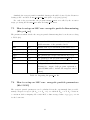
DIII-D discharge #122117 at t = 0.414 s. The parameter used are
Q0 = 3.9891D0, Q1 = 15.000D0, RL = 2.5D0, NREQ= 150, EPSILO=
0.360781991d0, BUMPEQ= 0.75D0, CG = 0.2000D0, WG = 0.220D0. . .
3
12
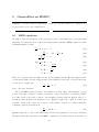
Fourier modes included in a HMGC simulation: (left) the n = 2 reference
DIII-D case, (right) a n = 2, 4 case. Black dots represent the modes
actually included in the simulations, the red crosses represent the modes
considered in the simulation because of complex conjugate condition. . .
4
16
Radially integrated magnetic energy of the perturbed Fourier components
vs. time: the flag (fourth column) in the TMODE PL input file commands
the Fourier components to be plotted. Note that here the result of a
simulation in which nout=100. is shown. . . . . . . . . . . . . . . . . . .
5
34
Example of integrated total energy Wtot−m,n vs. time. The labels on
the right of the plot, describing the (m, n) poloidal and toroidal mode
numbers of the curves, are written every two modes, because of space
limitation (although in the plot all the components are shown). . . . . .
6
36
Radial profiles of the Fourier components from CTBO file as produced by
the previous script (only the first 8 frames are shown): solid black line:
real part, dotted red line: imaginary part. . . . . . . . . . . . . . . . . .
7
Example for density, βH (red dashed curve is β⊥,H , green dotted curve is
βk,H ) and αH radial profiles. . . . . . . . . . . . . . . . . . . . . . . . . .
8
39
42
Frames number “161” (tωA0 = 96.) as produced by the program
plot field.f using the xplot field input data shown above. Left:
φ(r, θ, ϕ = 0). Centre: φ(r, θ, ϕ) and superimposed the position of the
first test particle (produced by assigning iflag test=1). Right: trajectories of the first test particle (rtest , θtest , ϕtest , utest ) (produced by assigning
iflag test=1 and iflag trajectory=1). . . . . . . . . . . . . . . . . .
47
9
Test particle trajectory projected on the poloidal cross section (ϕ = 0.,
the cross indicates r = 0) and on the equatorial plane (Z = 0, top
view of the torus, dotted line refers to r = 0, the cross indicates the
axis of symmetry of the torus) (produced by assigning iflag test=1 and
iflag trajectory=1). . . . . . . . . . . . . . . . . . . . . . . . . . . . .
10
Left:
48
φm,n (r) (produced by assigning iflag fourier comp=1 and
iflag contour=0). Centre: φm,n (r) (contour plot) and superimposed
the curve m = nq(r). Right: frequency spectra of φm,n in the plane (r, ω)
(contour plot) with superimposed the upper and lower Alfv´en continua
of the toroidal gap for a particular toroidal mode number (automatically
chosen from the first perturbed mode, in this case n = 2) (produced
by assigning itot=961, ipl0=ipl1=481, iflag power spectrum=1 and
other data from file xplot field input). . . . . . . . . . . . . . . . . . .
11
48
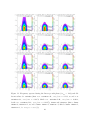
Frequency spectra during the linear growth phase (tωA0 = 144.) and
different values for twindow (first row: twindow=48., ωmin /ωA0 ' 0.131,
second row: twindow=96., ωmin /ωA0 ' 0.0654, third row: twindow=144.,
ωmin /ωA0 ' 0.0436, forth row: twindow=192., ωmin /ωA0 ' 0.0327),
ihann and ibuffer (first column: ihann=0, ibuffer=1, second column: ihann=1, ibuffer=1, third column: ihann=1, ibuffer=3, i.e.
ωmin,plot = ωmin /3). . . . . . . . . . . . . . . . . . . . . . . . . . . . . . .
12
49
Frequency spectra during the saturated phase (tωA0 = 432.) and
different values for twindow (first row:
twindow=72., ωmin /ωA0 '
0.0873, second row: twindow=144., ωmin /ωA0 ' 0.0436, third row:
twindow=288., ωmin /ωA0 ' 0.0218), ihann and ibuffer (first column:
ihann=0, ibuffer=1, second column: ihann=1, ibuffer=1, third column: ihann=1, ibuffer=3, i.e. ωmin,plot = ωmin /3). . . . . . . . . . . . .
13
Left:
fH (r, µ, u).
mesh.
rjer0
Centre:
Right: fH (r, E, α).
pl min
= 0.375 to rjer0
50
fH (r, µ, u) transformed on the (E, α)
All figures are obtained summing from
pl max
= 0.625. Note that the input file
xplot deltaf input shown in the text refers to the left plot; the figure in the centre is obtained with iflag versus=2; the figure on the
right is obtained reading the file deltaf ealfa.data. All figures refer to
the frame “1” (tωA0 = 0.). . . . . . . . . . . . . . . . . . . . . . . . . . .
52
14
Left: δfH (r, µ, u). Centre: δfH (r, µ, u) transformed on the (E, α) mesh.
Right: δfH (r, E, α). All figures are obtained summing from rjer0
0.375 to rjer0
pl max
pl min
=
= 0.625. The relaxed time is trelax = 120. With
respect to the input file xplot deltaf input shown in the text, the figures are obtained by assigning iflag df=1. All figures refer to the frame
“211” (tωA0 = 126.). . . . . . . . . . . . . . . . . . . . . . . . . . . . . .
15
52
Left: PH (r, µ, u). Also the curves representing the maximum energy
loaded in the initial distribution function (dotted lines) and the trappeduntrapped particle boundaries for the lower (solid line) and upper (dashed
line) radii considered are shown. Right: PH (r, E, α). All figures are obtained summing from rjer0
= 0.625. . . . . .
53
16
pperp /ppar vs. ∆. . . . . . . . . . . . . . . . . . . . . . . . . . . . . . . . .
56
17
Experimental profiles for the DIII-D shot # 122117. . . . . . . . . . . . .
59
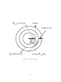
18
Beam geometry. . . . . . . . . . . . . . . . . . . . . . . . . . . . . . . . .
60
pl min
= 0.375 to rjer0
pl max
List of Tables
1
Parameters in the file EQUIPA. . . . . . . . . . . . . . . . . . . . . . . . .
10
2
Structure of the file EQNEW. . . . . . . . . . . . . . . . . . . . . . . . . . .
13
3
Structure of the file PARAM. . . . . . . . . . . . . . . . . . . . . . . . . . .
18
4
Structure of the file PARAM (continued). . . . . . . . . . . . . . . . . . . .
19
5
Structure of the file grid inc. . . . . . . . . . . . . . . . . . . . . . . . .
25
6
Structure of the file KININP. . . . . . . . . . . . . . . . . . . . . . . . . .
27
7
Structure of the file KININP (continued). . . . . . . . . . . . . . . . . . .
28
8
Structure of the file KININP (continued, 2). . . . . . . . . . . . . . . . . .
29
9
Quantities in the file ENERGY. . . . . . . . . . . . . . . . . . . . . . . . .
32
10
Experimental radial profiles provided by DIII-D team. . . . . . . . . . . .
58
11
Preparing the grid inc file. . . . . . . . . . . . . . . . . . . . . . . . . .
62
12
Preparing the KININP file. . . . . . . . . . . . . . . . . . . . . . . . . . .
63
HMGC User guide
1
Introduction
In a burning plasma, fast ions (MeV energies) produced by additional heating and/or
fusion reactions are expected to transfer their energy via Coulomb collisions to the
thermal plasma particles (10keV energies). Due to their high velocity, of the order of
Alfv´en velocity, they can resonate with and possibly destabilize Alfv´en modes. Energetic
ion transport and confinement properties – of crucial importance for achieving efficient
plasma heating and, therefore, ignition conditions – can in turn be affected by nonlinear
interactions with the Alfv´enic turbulence. Thus large efforts have been devoted to assess
the stability of shear-Alfv´en modes in tokamaks and to investigate their effect on the
energetic ion transport.
The need of fully retaining nonlinear dynamics and properly taking into account
kinetic effects, such as resonant interactions between energetic ions and Alfv´en modes
and the nonperturbative character of such interactions makes the numerical particlesimulation approach the natural tool for this investigation.
A hybrid MHD-particle 3-D simulation code, HMGC (Hybrid MHD Gyrokinetic
Code) has been developed in Frascati in the early 90’s.
The plasma model adopted in the HMGC code consists of a thermal (core) plasma
and an energetic-ion population. The former is described by reduced O(3 ) MagnetoHydro-Dynamics (MHD) equations in the limit of zero pressure ( being the inverse
aspect ratio of the torus), including resistivity and viscosity terms. The reduced MHD
equations expanded to O(3 ) allow us to investigate equilibria with shifted circular magnetic surfaces. The energetic-ion population is described by the nonlinear gyrokinetic
Vlasov equation [1, 2], expanded in the limit k⊥ ρH 1 (with k⊥ being the perpendicu-
7
lar component of the wave vector to the magnetic field, and ρH the energetic-ion Larmor
radius), though fully retaining magnetic drift orbit widths, and solved by particle-in-cell
(PIC) techniques. The coupling between energetic ions and thermal plasma is obtained
through the divergence of the energetic-ion pressure tensor, which enters the vorticity
equation. Numerical simulations of experimental conditions are performed by fitting
the relevant thermal-plasma quantities – the on-axis equilibrium magnetic field, major
and minor radii (R0 and a, respectively), the safety-factor q, the electron ne and ion
ni plasma densities, the electron temperature Te –, the anisotropy of the energetic-ion
distribution function and the ratio βH between fast ion and magnetic pressures.
In order to retain the relevant finite Larmor radius effects without resolving the
details of the gyromotion, the energetic ions are evolved in their gyrocenter coordinate
system, which corresponds to averaging the single-particle equations of motion over the
fast Larmor precession.
HMGC has been successfully applied to the interpretation of the experimental evidences of rapid transport of energetic ions related with fluctuations in the Alfv´en-mode
frequency range in auxiliary-heated JT-60U discharges, in connection with so called
Abrupt Large-amplitude Events (ALEs) [3, 4, 5]. HMGC results have also suggested a
possible justification of the large discrepancy, observed in reversed-shear beam-heated
DIII-D discharges, between the energetic particle radial density profile expected from
classical deposition and that deduced from the experimental measurements.
In spite of the slightly simplified physical model, HMGC has been getting increasing
attention from the international plasma physics community, and it has been recently
acquired by EPFL CRPP Lausanne, University of California Irvine and IFTS Zhejiang
University.
Aim of the present report is yielding a HMGC User Guide. We proceed with a
summary description of the various sections. In Sect. (2) it is shown how to produce a
plasma equilibrium needed by HMGC. In Sect. (3) it is described the execution script
which prepares the set of input files required for compilation and execution of the code.
In particular, the script prepares both the sets of files required by the two modules that
constitute the hybrid code: the MHD module and the gyrokinetic one. Sects. (4) and
(5) describe the output files of the MHD part and of the gyrokinetic one, respectively;
they also describe the suite of graphics tools used to post-process and visualize the
results contained in these files. Sect. (6) describes the three types of energetic particles
distribution functions that can be loaded to start a simulation: the slowing down, the
8
maxwellian and the bi-maxwellian distribution functions. The various operations needed
to setup a run of HMGC have been collected in Sect. (7), where a specific HMGC run
referred to a DIII-D, beam-heated discharge is used as an example. Sect. (8) shows the
list of the directories tree structure of HMGC. Finally, in Sect. (9) several excerpts of
Ref. [9] are reported to illustrate the analytical details of the model that constitutes the
basis of HMGC.
2
How to produce an MHD equilibrium file
The equilibrium file required by HMGC is produced by running the fortran file eqe3aaab.
This program solves the Grad-Shafranov equation expanded to the O(3 ) in the inverse
aspect ratio ≡ a/R0 , with a and R0 the minor and major radius of the torus, respectively for the poloidal flux function ψ (see Sect.(9)), assuming an analytic parametrization of the safety factor profile q = q(r) (with r the normalized minor radius r ≡ r/a, a
being the minor radius of the circular cross section torus) given by:
"
q(r) = q0 1 +
r
r0
2λ #1/λ
,
(1)
with r0 defined in terms of λ and the q value at the centre q(r = 0) ≡ q0 and at the
edge q(r = 1) ≡ qa :
r0 =
λ
qa
q0
−1/2λ
.
−1
(2)
The normalized (to BT /R0 ) current density profile and the shear profile can be
derived from the previous expressions:
2
j(r) =
q0 1 +
sˆ(r) =
r
r0
2λ λ1 +1
,
(3)
r
r0
2λ
1+
2
2λ ,
(4)
r
r0
From the above expressions the normalized (to BT a2 /R0 ) Fourier components ψm,0
for the equilibrium poloidal flux function are obtained, namely ψ0,0 , ψ1,0 (here m is
the poloidal mode number, and the toroidal mode number n = 0 has been assumed
9
for the axisymmetric equilibrium). Please note that the normalizations in the
gyrokinetic module will be different.
The expressions shown in eqs. (1), (2) (3) (4) are appropriate for describing a monotonic q-profile, but they are inadequate to describe more general safety factor profiles,
as, e.g., reversed shear profiles. Thus a number of bumps on the current density profile
can be superimposed on eq. (3). Actually up to 3 bumps can be superimposed:
„
2
j(r) =
q0 1 +
2λ λ1 +1
r
r0
+
X
−
bumpeq,i e
r 2 −cgi
wgi
«2
,
(5)
i=1,3
where bumpeq,i can be positive or negative. The current density profile resulting from
Eq.(5) is then rescaled and such to provide a q profile which has the minimum equal to
the parameter q0 of Eq. (1).
The meaning of the different parameters of the input file (EQUIPA) (assigned as a
namelist with the same name of the input file) are listed in Table (1).
Q0
minimum q value
Q1
maximum value of q at r/a = 1: qa (if bumpeq,i = 0)
RL
λ
NREQ
Number of points in the radial mesh
NMESHA
parameter of non equally spaced mesh (usually not used)
NPOIDA
parameter of non equally spaced mesh (usually not used)
SOLPDA
parameter of non equally spaced mesh (usually not used)
APLACE(i)
parameters of non equally spaced mesh (usually not used)
AWIDTH(i)
parameters of non equally spaced mesh (usually not used)
EPSILO
inverse aspect ratio ( ≡ a/R0 )
RHOFLG
logical value, if .true. compute η(r)/η0 = j0 /j(r)
BETA0
parameter for equilibrium pressure profile (usually not used)
C1, C2, C3, C4, C5
parameters for equilibrium pressure profile (usually not used)
BUMPEQ, CG, WG
bumpeq,1 , cg1 , wg1
BUMPEQ1, CG1, WG1
bumpeq,2 , cg2 , wg2
BUMPEQ2, CG2, WG2
bumpeq,3 , cg3 , wg3
ireadcur
parameter to read current density profile as alternate input
Table 1: Parameters in the file EQUIPA.
10
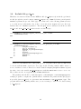
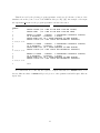
To help in fitting an experimental q-profile, an utility to compare the experimental
profile with the one obtained with the program eqe3aaab is provided (program
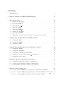
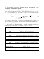
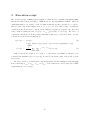
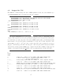
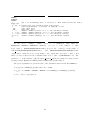
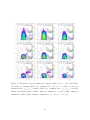
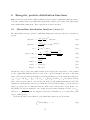
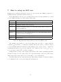
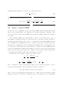
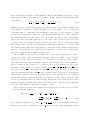
plot equil, see fig. (1)). In figure (1) the effect of including or not including the
bumps in the current profile is shown (&EQUIPA Q0 = 2.4110D0, Q1 = 5.1280D0,
RL = 4.0D0, EPSILO = 0.293217665d0, BUMPEQ = 1.30D0, CG = 0.4000D0, WG =
0.350D0, bumpeq1 = -2.20D0, cg1 = 0.90D0, wg1 = 0.30D0, &END). Please note
that peculiar shaping of the current density profile should be avoided as much as
possible, in order to prevent the (not desirable) growth of MHD unstable modes. Note
that a positive bump in the current profile is used to produce an off-axis minimum in
the q-profile, whereas a positive bump at the edge is used to “pull-up” the q-profile at
the edge.
ITER-SC4-no-bumps
ITER-SC4-bumps
Figure 1: ITER-SC4 q-profile example of use of current bumps: (left) no bumps, (right)
with two bumps (one bump is positive in amplitude (BUMPEQ = 1.30D0) located at r2 =
CG = 0.4000D0 (r ' 0.632) having width WG = 0.350D0 and the second is negative
(bumpeq1 = -2.20D0) at r2 = cg1 = 0.90D0 (r ' 0.949) having width wg1 = 0.30D0).
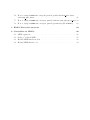
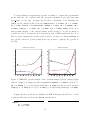
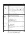
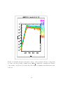
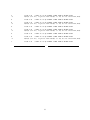
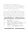
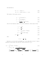
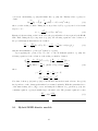
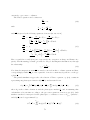
In figure (2) the q profile used to simulate the DIII-D discharge #122117 at t = 0.414
s is shown. Hereafter it follows the EQUIPA namelist used:
...
&EQUIPA
Q0 = 3.9891D0,
Q1 = 15.000D0,
11
RL = 2.5D0,
NREQ= 150,
NMESHA =
0,
NPOIDA =
2,
APLACE(1) = 0.426D0, 0.9D0, 0.00D0, 0., 0., 0., 0., 0., 0., 0.,
AWIDTH(1) = 0.100D0, 0.10D0, 0.00D0, 0., 0., 0., 0., 0., 0., 0.,
SOLPDA = 0.60D0,
EPSILO= 0.360781991d0,
RHOFLG=.FALSE.,
BETA0 = 0.00000D-0,
C1
= -1.7438D0,
C2
= -2.3515D0,
C3
= 12.01D0,
C4
=-15.988D0,
C5
= 7.3964D0,
BUMPEQ= 0.75D0,
CG
= 0.2000D0,
WG
= 0.220D0,
bumpeq1 =-0.00D0,
cg1
= 0.90D0,
wg1
= 0.30D0,
bumpeq2 =-0.00D0,
cg2
= 0.95D0,
wg2
= 0.20d0,
ireadcur= 0,
&END
...
ITER-DIII-D-1
Figure 2:
DIII-D discharge #122117 at t
=
0.414 s.
The parame-
ter used are Q0 = 3.9891D0, Q1 = 15.000D0, RL = 2.5D0, NREQ= 150, EPSILO=
0.360781991d0, BUMPEQ= 0.75D0, CG = 0.2000D0, WG = 0.220D0.
The output of the program eqe3aaab is a file named EQNEW. This file will be copied by the
HMGC execution script to the file named INCOND. Its structure is shown in table (2).
12
Quantities
Comments
the EQUIPA namelist
see Table (1)
0.D0
FORMAT(3I20), NR is the number of radial grid
NR, 1, 0
points
FORMAT(2D30.15) the normalized radial coordi-
R(I), I=1,NR
nate
a sequence of radial profiles for the (m = 0, n = 0)
and (m = 1, n = 0) Fourier components for ψ, φ
and resistivity profile η in the following format:
two blank lines
a line containing the following text:
PSI 1
PSI 1 for ψm,n (r),
PHI 3 for φm,n (r) or
RES 4 for ηm,n (r)
real(m), real(n)
FORMAT(2F20.0), m, n being the poloidal and
toroidal mode numbers, respectively (for the equilibrium is n = 0)
real(ψm,n (I)), imag(ψm,n (I))
FORMAT(2E30.15),
I=1,NR+1 (only NR points
for φ and η)
Table 2: Structure of the file EQNEW.
13
Note that here n = 0 (equilibrium); also note that the ψm,n (r) harmonics have one more
radial point (NR+1) corresponding to the position of a resistive wall (this option is usually
not considered). The electrostatic scalar potential φm,n (r) components for the equilibrium are
identically zero (equilibrium without fluid flow), and usually (MHD module of HMGC used in
linear mode) the resistivity profile is taken constant in radius (η0,0 = 1, η1,0 = 0). Note also
that HMGC defines the ψ0,0 to be ψ0,0 (r = 1) = 0 and positive in the plasma.
14
3
Execution script
The execution script of HMGC prepares a number of files used for compiling and running HMCG.
Hereafter is a list of them, referring to a DIII-D case (see fig. (2)) simulation which consider an
equilibrium with m = 0, 1 and n = 0 modes (this is mandatory) and a perturbed n = 2 mode,
with poloidal components ranging from m = 1 to m = 21. Note that because of symmetry
conditions in the Fourier space, only modes in a half (m, n) plane are required, the other ones
∗
being considered using the rule ψm,n (r) = ψ−m,−n
(r) (reality of ψ(r, θ, ϕ)). The choice of
considering only the mode in the positive half plane defined by n ≥ 0 is used. More over, the
conventions for the Fourier transform are:
ψ(r, θ, ϕ) = ψ0,0 (r) +
X
2
[Re(ψm,n (r)) cos(mθ − nϕ) − Im(ψm,n (r)) sin(mθ − nϕ)] ,
(6)
l=2,LM
ψm,n (r) =
X
1
Nθ Nϕ
X
e−i(mθj −nϕk ) ψ(r, θj , ϕk ) ,
(7)
j=1,Nθ k=1,Nϕ
with l being the mode index, m = m(l), n = n(l), LM the total number of Fourier components in the simulation (see Sect. (3.4)), Nθ and Nϕ the mesh points of the θ and ϕ grids,
respectively.
The choice for the poloidal Fourier components included in the simulation derives usually
from considering mmin ≈ nqmin , mmax ≈ nqmax . Some restrictions could be imposed by FFT
requirements (see Sect. (3.1)).
15
3.1
Include file modi inc
Parameter definitions for compiling the MHD module (e3 complete.F) of HMGC. NR is the
MHD radial grid (must be NR=NREQ, see Table (1)). LM is the number of Fourier components
considered in the simulations. NMAX=nmax + 1 is the maximum toroidal mode included in the
simulation n plus unity. MMAX is the maximum number of poloidal Fourier components for
fixed toroidal mode number n. MAXPRI is a parameter to dimension a buffer for certain output
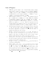
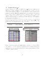
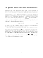
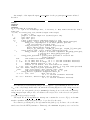
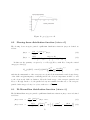
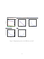
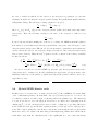
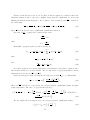
quantities. In Fig. (3) are shown two sketches of the (m, n) plane used by HMGC, for better
clarify the parameters meaning. A constraint given by FFT routines impose that 4*(MMAX-1)
is a valid number for the FFT (see, e.g.,
http://publib.boulder.ibm.com/infocenter/clresctr/vxrx/topic/com.ibm.cluster.essl43.guideref.doc/am501 formul2.html).
Actually, the IBM ESSL package is used, but routines which use NAG modules are also
included in the source files (although they could be out of date).
...
PARAMETER
(NR=150,NMAX=3,MMAX=21,LM=23,MAXPRI=200)
...
m_n2_sim
m_n2_cc
m_n0_sim
m_n0_cc
m_n2_sim
m_n2_cc
TMODE-1
NMAX=2+1
0
-1
-2
-20 -15 -10
-5
MMAX=21
0
2
c.c. modes not explicitly
included in the simulation
LM=23
NMAX=4+1
0
-2
-4
5
10
15
-15
20
m
{
{
{
{
4
n
n
1
LM=23
{
2
m_n4_sim
m_n4_cc
TMODE-1
-10
-5
MMAX=14
{
m_n0_sim
m_n0_cc
0
c.c. modes not explicitly
included in the simulation
5
10
15
m
Figure 3: Fourier modes included in a HMGC simulation: (left) the n = 2 reference DIII-D
case, (right) a n = 2, 4 case. Black dots represent the modes actually included in the
simulations, the red crosses represent the modes considered in the simulation because
of complex conjugate condition.
16
3.2
Input file PARAM
This input file contains the main input parameters for the MHD module, and for some general
input parameters for the simulation. Here is a sample for the DIII-D simulation (see also
Tables (3), (4)):
...
160
3
20
92
1.0D-5
1.0D-8
0.02
30
1.000001
NCYCLE
NSUBCY
NOUT
LR1
ETA
VISC
DT
NPRI
RWALL
1.0D10
TAUWAL
0.0D00
VEDGE
Number of GK calls; Number of Time Steps NTS=NCYCLE*NSUBCY
Number of MHD calls per each GK call
Number of time sequences; total time steps=NTS*NOUT
Maximum value should be LR1=4*LM
standard value: 1.0d-5
standard value: 1.0d-8
standard value: 0.02
NTS/NPRI<=MAXPRI
resistive wall normalized radius
(parameter required but not used by fortran, give any real number)
resistive wall characteristic time
(parameter required but not used by fortran, give any real number)
plasma bulk velocity at the edge
(parameter required but not used by fortran, give any real number)
current ramp (now ignored)
l=1 (m,n)=(0,0)
l=2 (m,n)=(1,0)
0.0D00
CURAMP
.TRUE.
FREZ00
.TRUE.
FREZ10
.FALSE.
EQUIL
.FALSE.
DROP
1
NPROFI 0 DEN=1; 1 DEN=DEN(RHOA,ALFA,BETA); 2 DEN=(Q/Q0)**(-2)
3.9173d0 ALFA
0.69776d0 BETA
0.6471d0 RHOA
0.7
AGROWTH ad hoc growing factor parameter
0.01
BGROWTH ad hoc growing factor parameter
0.05
CGROWTH ad hoc growing factor parameter
0.95
DGROWTH ad hoc growing factor parameter
1
ITAERSP 1 drives TAE, 2 drives RSP (requires GROWTH .ne. 0)
1.D0
SMOFAC amplitude of the smoothing factor
(1.D-07,1.D-07) AMP complex amplitude factor for the initial perturbation
0.00D-0
GROWTH amplitude of the ad hoc growing term
.TRUE.
GYRO
call gyrokinetic module
.FALSE.
CYLIN
.true. MHD cylindrical limit
.FALSE.
BISEC
.true. bisection allowed
0.D-2
SKIN
(el. skin depth; skin=0.D0 ==> el. inertia neglected)
0.10d0
epsil1 parameter used to reduce toroidal corrections at the edge
0.95d0
cgeps
parameter used to reduce toroidal corrections at the edge
0.025d0
cweps
parameter used to reduce toroidal corrections at the edge
$DIAPOS
NRCHNL=6,
RCHNL(1)=0.200,
RCHNL(2)=0.300,
RCHNL(3)=0.400,
RCHNL(4)=0.500,
RCHNL(5)=0.650,
RCHNL(6)=0.800,
&END
...
17
Quantities
Comments
NCYCLE
number of calls of the gyrokinetic module for each of the NOUT time
sequences
NSUBCY
Number of MHD calls per each gyrokinetic call; NCYCLE*NSUBCY is the
number of calls of the MHD module for each of the NOUT time sequences
NOUT
number of time sequences; total time steps=NCYCLE*NSUBCY*NOUT
LR1
maximum number of modes per MHD fields which are read in the file
INCOND: maximum value should be LR1=4*LM
ETA
normalized resistivity, i.e. the inverse of the Lundquist number S (the
ratio between resistive and Alfv´en times S ≡ τη /τA0 , with τη = µ0 a2 /η
−1
and τA0 ≡ ωA0
)
VISC
similar to ETA parameter, but representing viscosity
DT
elementary time step
NPRI
some outputs are performed every NPRI time steps; NPRI must satisfy
NTS/NPRI<=MAXPRI
RWALL
resistive wall normalized radius (parameter required but not used by
fortran, give any real number)
TAUWAL
resistive wall characteristic time (parameter required but not used by
fortran, give any real number)
VEDGE
plasma bulk velocity at the edge (parameter required but not used by
fortran, give any real number)
CURAMP
current ramp (only significant if “equilibrium” is evolved)
FREZ00
logical variable, if .true. does not evolve (“freeze”) l=1 mode (0,0)
FREZ10
logical variable, if .true. does not evolve (“freeze”) l=2 mode (1,0)
EQUIL
logical variable, if .true. the code is used to compute an “equilibrium”
(useful for nonlinear MHD runs)
DROP
logical variable, if EQUIL=.true. and DROP=.true. kinetic energy is
removed by dropping φm,n by a fixed factor (useful for preparing nonlinear
MHD runs)
Table 3: Structure of the file PARAM.
18
Quantities
Comments
NPROFI
switch for assigning the bulk density radial profile ρˆ: NPROFI=0 → ρˆ = 1;
NPROFI=1 → ρˆ = ρˆ(α, β, ρa ); NPROFI=2 → ρˆ = [q(r)/q(0)]−2 (aligned
toroidal gap)
ALFA,
ρˆ(α, β, ρa ) = (1 − ρa ) ∗ (1 − rα )β + ρa
BETA, RHOA
AGROWTH,
parameters
for
BGROWTH,
in
the
CGROWTH,
cle
drive):
DGROWTH
GROWTHR(I)=GROWTH*EXP(-((R(I)-AGROWTH)**2/BGROWTH)),
vorticity
for
an
“ad
equation
CGROWTH
hoc”
growing
term
added
(to
simulate
some
parti-
≤
r
≤
(CGROWTH+ DGROWTH):
else
GROWTHR(I)=0 (now obsolete)
ITAERSP
ITAERSP=1 should drive a (1,1), (2,1) TAE using the “ad hoc” driving
term, ITAERSP=2 should drive a (1,1), (2,1) RSP (Resistive Shear Periodic
mode), requires GROWTH.ne.0.0 and n = 1, m = 1, 2 modes
SMOFAC
amplitude of a “smoothing” factor to control numerical instabilities in
the center (r=0) (hyper-resistivity and hyper-viscosity terms)
AMP
complex amplitude factor for the initial perturbation
GROWTH
amplitude of the “ad hoc” growing factor
GYRO
logical variable, ifGYRO=.true. the gyrokinetic module is called
CYLIN
logical variable, ifCYLIN=.true. MHD module considers cylindrical limit
while gyrokinetic module retains finite correction
BISEC
logical variable, ifBISEC=.true. allow time bisection in the MHD module (and, hence, in the gyrokinetic one)
SKIN
electron skin depth (if 0, electron inertia neglected, now obsolete, not
used)
epsil1
parameter used to reduce correction at the edge (occasionally used
to control edge numerical instabilities arising from MHD module, see
Eq. (8))
cgeps
parameter used to reduce correction at the edge (see Eq. (8))
cweps
parameter used to reduce correction at the edge (see Eq. (8))
namelist
NRCHNL=6 diagnostic output channels, at the radii RCHNL(i=1,6), giving
DIAPOS
Real and Imaginary part of φm,n (rchnl , t).
Table 4: Structure of the file PARAM (continued).
19
The general time stepping in HMGC is as follow: the MHD (normalized) time step is given
by the parameter DT. Each NSUBCY MHD time steps, the gyrokinetic module is called. This
loop is performed NCYCLE times. Thus a total umber of time steps of NTS=NCYCLE*NSUBCY
is performed for each time sequence. This time sequence is repeated NOUT times. Thus, the
total number of time steps of a simulation is Ntime−steps = NTS*NOUT = NCYCLE*NSUBCY*NOUT
and the total (normalized) time simulated is Ttotal = DT*NCYCLE*NSUBCY*NOUT. Schematically,
using a fortran-like schema, these nested loops are as follows:
...
time=0.
do i=1, NOUT
do j=1,NCYCLE
call GyroKinetic module
do k=1,NSUBCY
time=time+dt
call MHD module
enddo
enddo
enddo
...
The time is normalized to the inverse of the on-axis (r = 0) Alfv´en frequency, that
is tcode = t(s)ωA0 (s−1 ) with ωA0 ≡ vA0 /R0 and vA0 the on-axis Alfv´en velocity. If
FREZ00=.true. and FREZ10=.true. (no evolution of equilibrium components) and a single perturbed n is included in the simulation, a linear MHD simulation will be performed:
this is the usual operation condition of the MHD module. The parameters epsil1, cgeps and
cweps are used to define a radial function f (r) which modulates the toroidal corrections:
r − cg
1 − 1 /
tanh
+1 ,
f (r) = 1 −
2
cw
f (r) −→ 1
for
r cg
f (r) −→ 1 /
r cg .
for
20
(8)
3.3
Input file stop run
At the beginning, this file contains only one line, which can be used to overwrite the parameter
NOUT given in the file PARAM:
...
20 nout_new
...
At run time, the same file is written and read by HMGC and this allows to stop or extend
the run by editing it and changing the parameter nout:
...
25 nout
21 ncount
192.0000000
time
...
Here ncount is the actual number of time sequences performed by the code and time is
the corresponding normalized simulation time.
21
3.4
Input file TMODE
This input file contains the list of the Fourier modes actually included in the simulation. The
first column is the mode index l, running from l = 1 to l = LM. In the second and third columns
are listed the corresponding poloidal (m = m(l)) and toroidal (n = n(l)) mode numbers. It is
assumed that the modes are ordered by increasing n, and for each n by increasing m.
...
1
2
3
4
5
6
7
8
9
10
11
12
13
14
15
16
17
18
19
20
21
22
23
0
1
1
2
3
4
5
6
7
8
9
10
11
12
13
14
15
16
17
18
19
20
21
0
0
2
2
2
2
2
2
2
2
2
2
2
2
2
2
2
2
2
2
2
2
2
...
22
3.5
Input file TMODE PL
This input file is used by the plot post-processing program epe3ak31.u. It is exactly the
same than the input file TMODE, with the add of a fourth column, in which 0 means that
this component will not be considered by the plot program, whereas 1 means that it will be
considered.
...
1
2
3
4
5
6
7
8
9
10
11
12
13
14
15
16
17
18
19
20
21
22
23
0
1
1
2
3
4
5
6
7
8
9
10
11
12
13
14
15
16
17
18
19
20
21
0
0
2
2
2
2
2
2
2
2
2
2
2
2
2
2
2
2
2
2
2
2
2
0
0
1
1
1
1
1
1
1
1
1
1
1
1
1
1
1
1
1
1
1
1
1
...
23
3.6
Include file grid inc
This lines of fortran are included in the MHD module (e3 complete.F) and in the gyrokinetic
module (trough the general common commr31 complete.F) of HMGC. It defines general particle
simulation parameters (see also Table (5)). Note that some of the following parameters refer
to toroidal and poloidal meshes, also if the code is run in the nogrid mode (see Ref. [6]).
Particles here are “simulation particles”. The file grid inc is constructed from the two files
nlr inc and altri grid inc 1 written in the execution script:
...
cat >${HOMEroot_sources}/${pwr}_version/nlr_inc <<’EOF’
PARAMETER(nlr=64)
EOF
...
...
cat >${HOMEroot_sources}/${pwr}_version/altri_grid_inc_1 <<’EOF’
PARAMETER(NTH=168,
&
nintphi=2*(nmax-1),
&
nph_su_nintphi=4,
&
NPH=nph_su_nintphi*nintphi,
&
ippc=2,
&
nne=672,
&
npart=nlr*nth*nph*ippc**3,
&
NMODOM=27,
&
NRZ=5)
EOF
...
Please note that NLR should be NLR ≤ NR (see Sect. (3.1) where NR is defined). NTH should
be chosen such that NTH > 2mmax (see Sect. (3)): in the following example, NTH = 8mmax =
8 ∗ 21 = 168 has been used. The factor 2 in the variable nintphi (nintphi=2*(nmax-1)) and
the value of 4 for the variable nph su nintphi are such that NPH is NPH = 8nmax = 8 ∗ 2 = 16.
Those values are the ones typically used in HMGC simulations.
The quantity nne should be such that npart = nne*nnalpha = nlr*nth*nph*ippc**3:
a simple program to compute the optimal values to distribute the particles in the (E, α) space
is provided (calcolo nne.f), for given nlr, nth, maximum n, nph su nintphi, ippc. The
program asks at the beginning which source you are referring to: enter “0” for data referring
to e3 complete.
24
Quantities
Comments
NLR
number of radial cells for the gyrokinetic module (NLR+1 mesh
points)
NTH
number of points in the θ (poloidal angle) direction
nintphi
nintphi=2*(nmax-1).
Parameter for ϕ (toroidal angle) mesh:
the energetic particle distribution function will be loaded on
nph su nintphi toroidal mesh points and then replicated on
nintphi-1 remaining sectors
nph su nintphi
parameter for ϕ (toroidal angle) mesh
NPH
NPH=nph su nintphi*nintphi: number of points in the ϕ (toroidal
angle) direction
ippc
number of particles per cell in each direction of the physical space
(r, θ, ϕ)
nne
number of particles in the energy space (nne*nnalpha =
npart/nintphi, nnalpha is the number of particles in the pitch
angle direction)
npart
nlr*nth*nph*ippc**3: total number of particles
NMODOM
number of Fourier components for the gyrokinetic module: they
must be the Fourier modes of the MHD module plus two poloidal
satellite modes for each toroidal mode considered in the simulation
NRZ
the particles are evolved in a (NRZ,NRZ) grid in the (R, Z) plane
around the r = 0 point to avoid problems related to the singular
point r = 0 in polar coordinates.
Table 5: Structure of the file grid inc.
25
3.7
Input file KININP
This file is the main parameter input for the gyrokinetic module. Here is a sample for the
DIII-D simulation (see also Tables (6), (7)):
...
idistr=1: sqrt(T_H0/m_H)/Omega_cH0/a;
idistr=2: sqrt(E_0/m_H)/Omega_cH0/a;
idistr=3: sqrt(T_perp_H0/m_H)/Omega_cH0/a
VTHSVA
idistr=1: sqrt(T_H0/m_H)/v_A0;
idistr=2: sqrt(E_0/m_H)/v_A0);
idistr=3: sqrt(T_perp_H0/m_H)/v_A0
sigma_0
idistr=3: T_perp_H0/T_par_H0
usdelta_input
idistr=1,2: anisotropy parameter (1/width)
cosalfa_0_input idistr=1,2: anisotropy parameter
(cosine of injection pitch angle)
e0sec0
idistr=2: on-axis E0/E_crit0
ALF
parameter controlling non uniform radial
particle loading
NPIC
parameter controlling non uniform radial
particle loading
(if npic.ne.0, er0(i), del(i), i=1,npic must follow)
ENHSNI
n_H0/n_i0 on axis ratio between energetic particle
and bulk ion densities
EMHSMI
m_H/m_i
ratio between energetic particle and bulk
ion masses
timkin_anu
energetic particle density ramps for t > timkin_anu
(set to a large value to avoid ramping)
TIMKIN_RELAX
time at which the distribution function is assumed
to be relaxed; used for ramping and diagnostics
ANU_MAX
energetic particle density ramping parameter
ANU_DOT_0
energetic particle density ramping parameter
i_write_deltaf 0: no output,
1: output of f(r,mu,u,t),
2: output of f(r,E,alpha,t)
i_write_power
0: no output,
1: output of wave-particle power exchange P(r,mu,u,t)
NWRITE
energetic particle quantities written every
NWRITE time steps
IDISTR
1: Maxwellian, 2: Slowing-down, 3: bi-Maxwellian
IDELTF
0: full f, 1: delta-f
ILIN
0: fully non linear GK simulation,
1: linear GK simulation
IRLSR0
0: R_l with epsilon corrections, 1: R_l=R0
IMIRR
0: mirroring term off, 1: mirroring term on
IW00
0: grad-B drift contribution to the source term
neglected, 1: retained
ILANDA
0: Landau damping term off, 1: Landau damping term on
ICURV
0: curvature term off, 1: curvature term on
IOMST
0: omega-star term off, 1: omega-star term on
NPTEST
number of test particles
ITEST
0: true test particle, 1: simulation particle
ER0T,TH0T,PH0T,AM0T,U0T for t=0: r,theta,phi,mu,u
ITEST
0: true test particle, 1: simulation particle
LTEST
simulation particle identification number
ER_PERT0:
energetic particle pressure term PREK set to
zero for r<er_pert0
l, iprek(l)
iprek(l)=0: l-th Fourier component of the PREK off,
iprek(l)=1: on
l, iprek(l)
0.032863457d0 RHOSA
0.271063836d0
1.5d0
2.3256d0
0.68128d0
4.153850158d0
.2D00
0
0.264848976d0
1.D00
999.99d9
120.d0
1.166212d0
0.166212d-2
0
0
30
2
1
0
0
1
1
1
1
1
2
0
.5,0.,0.,.1,1.
1
1352
0.
1 1
2 1
...
26
Quantities
Comments
RHOSA
ρH /a: particle Larmor radius normalized to minor radius computed:
(1) at the on-axis energetic particle temperature TH0 (ρH /a =
p
( TH0 /mH /ΩcH0 )/a if a Maxwellian distribution is considered,
IDISTR=1);
p
(2) at the birth energy E0 (ρH /a = ( E0 /mH /ΩcH0 )/a) if a slowing
down distribution function is assumed, IDISTR=2);
(3) at the on-axis perpendicular energetic particle temperature
p
T⊥,H0 (ρH /a = ( T⊥,H0 /mH /ΩcH0 )/a if a bi-Maxwellian distribution is considered, IDISTR=3)
VTHSVA
vth /vA0 : ratio between energetic particle thermal velocity and onaxis Alfv´en velocity:
p
TH0 /mH /vA0 ;
p
= E0 /mH /vA0 ;
p
= T⊥,H0 /mH /vA0
for IDISTR=1: vth /vA0 =
for IDISTR=2: vth /vA0
for IDISTR=3: vth /vA0
sigma 0
ratio between on-axis perpendicular and parallel energetic particle
temperatures (used only if IDISTR=3)
usdelta input
parameter for anisotropic particle distribution function, it corresponds to the inverse of the width ∆ (see Sects. (6.1), (6.2)) of
the distribution function around the injection pitch angle α0 for
Maxwellian or slowing down distribution functions (IDISTR=1 or
IDISTR=2)
cosalfa 0 input cos α0 , cosine of the injection pitch angle α0 for Maxwellian or slowing down distribution functions (IDISTR=1 or IDISTR=2)
e0sec0
E0 /Ecrit,0 , on-axis ratio between birth energy and critical energy
for slowing down distribution function (IDISTR=2)
ALF
parameter for non uniform energetic particles radial loading: uniform fraction, 0<ALF<1
NPIC
parameter for non uniform energetic particles radial loading: number of gaussians overimposed to the uniform distribution fraction
ALF.
ER0(I),DEL(I)
If NPIC.ne.0 the corresponding values of the radial positions and
widths (ER0(I),DEL(I)) of the gaussians must be given
Table 6: Structure of the file KININP.
27
Quantities
Comments
ENHSNI
nH0 /ni0 , on-axis ratio between the energetic particle and bulk ion
densities
EMHSMI
mH /mi , ratio between the energetic particle and bulk ion mass
timkin anu
parameter for ramping the energetic particle density: energetic particle density ramps for t > timkin anu. timkin anu should be
greater than TIMKIN RELAX but smaller than the time at which non
linear phase occurs. Set timkin anu greater than the total simulation time to avoid ramping
TIMKIN RELAX
time at which the energetic particle distribution function is assumed
to be relaxed (because of initialization of the distribution function
in terms of non conserved quantities)
ANU MAX
parameter for ramping the energetic particles: multiplying factor
of the normalized energetic particle density
ANU DOT 0
parameter for ramping the energetic particles: time derivative of
the normalized energetic particle density
i write deltaf
produces the output of the distribution function:
i write deltaf=0: no output is produced,
i write deltaf=1: f (r, µ, u, t),
i write deltaf=2: f (r, E, α, t)
(µ, u, E and α are the magnetic moment, parallel velocity, particle
energy and pitch angle, respectively)
i write power
flag for writing the power exchange P (r, µ, u, t) between particles
and waves:
0: no output is produced,
1: output is produced
NWRITE
energetic particle quantities are written on output files every
NWRITE*NSUBCY time steps
IDISTR
1: Maxwellian,
2: Slowing-down,
3: bi-Maxwellian
IDELTF
0: performs a full-f simulation,
1: performs a δf simulation (standard use of HMGC)
Table 7: Structure of the file KININP (continued).
28
Quantities
Comments
ILIN
0: performs a gyrokinetic non-linear simulation (standard use of
HMGC),
1: performs a gyrokinetic linear simulation
(note that ILIN=1 corresponds exactly to a linear simulation only
if the initial distribution function is a true equilibrium function)
IRLSR0
for the generic l simulation particle:
0: retains corrections Rl = R0 (1+l cos θl ) (standard use of HMGC),
1: approximates Rl = R0
IMIRR
0: mirroring terms off,
1: mirroring terms on (standard use of HMGC)
IW00
IW00=0 causes to neglect the contribution of the grad-B drift to
the source term in the delta-f Vlasov equation
1: terms are retained (standard use of HMGC)
ILANDA
0: Landau damping off,
1: Landau damping on (standard use of HMGC)
ICURV
0: curvature term off,
1: curvature term on (standard use of HMGC)
IOMST
0: ω∗ term off,
1: ω∗ term on (standard use of HMGC)
NPTEST
number of test particles
ITEST
for each test particle enter:
0: to initialize a true test particle,
1: to follow a simulation particle
5 reals,
if ITEST=0, the initial coordinates (t = 0) of the test particle must
or
be given (rtest , θtest , ϕtest , µtest , utest ),
LTEST
if ITEST=1, particle identification number
ER PERT0
energetic particle pressure tensor term (PREK) set to zero for r ≤
ER PERT0 (standard use of HMGC: ER PERT0=0)
l, iprek(l)
PREK(l)=0: lth Fourier component inactive,
PREK(l)=1: lth Fourier component of the energetic particle pressure
tensor term active (defaults is all Fourier components active)
Table 8: Structure of the file KININP (continued, 2).
29
3.8
Input files: energetic particle density and temperature profiles
Normalized (to the on-axis value) energetic particle density profile and temperature (if
Maxwellian distribution function is loaded, idistr=1), Ecrit (if slowing down distribution
function is loaded, idistr=2) or perpendicular and parallel temperatures (if bi-Maxwellian
distribution function is loaded, idistr=3) profiles must be provided on an equally spaced
normalized poloidal flux function grid ψ. These profiles are usually provided by standard
transport codes (e.g., available in the ITER database). If experimental profiles are provided
p
(e.g., ρ, q(ρ), nH (ρ), Te (ρ), TH (ρ)), as functions of ρ ≡ Φ/Φlimiter , the usual radial-like coordinate of transport codes (e.g., TRANSP) with Φ the toroidal magnetic flux function, a
simple program is provided (psi from rho q exp.f) which returns the poloidal flux function
ψ in terms of ρ, integrating the following expression:
2πdψ =
dΦ
,
q(ρ)
(9)
to obtain ψ = ψ(ρ). The normalized coordinate proportional to the poloidal flux function
should be such that it is zero in the centre and unity at the edge.
Those profiles will be interpolated using splines on the desired equally spaced normalized ψ mesh by the fortran program interp spline.f. “Experimental” files with ψnorm (ρ),
nH,norm (ρ) (and similar for the other quantities) must be provided (their names are, e.g.,
den exp DIII D 1, temp exp DIII D 1, temp exp par xxx, where temp exp DIII D 1 contains
the energetic particle isotropic temperature in the case idistr=1, the Ecrit normalized profile
in the case idistr=2, or the energetic particle perpendicular (temp exp DIII D 1) and parallel
(temp exp par xxx) temperature profiles in the case idistr=3). Then a corresponding output
on the equally spaced ψnorm mesh will be produced.
30
4
Output files: produced by the MHD module
4.1
Output file CTTO
The CTTO file has exactly the same form of the INCOND file, but includes all the Fourier components.
4.2
Output file ENERGY
The ENERGY file contains the four namelists params, diapos, equipa, paramk. Then it contains
a time sequence of some global fluid quantities, namely:
...
WRITE(CHENER,00003)
&
TIMBUF(JTBUF),LM,EZBUF(JTBUF),Q0BUF(JTBUF),
&
QABUF(JTBUF),2.*QABUF(JTBUF)**2*ENMODE(JTBUF,1,1),
&
(ENBUF(JTBUF,I),I=1,4),
&
(RM(L),RN(L),(ENMODE(JTBUF,K,L),K=1,IDIAGN+2),L=1,LM)
00003 FORMAT(F16.6,I6,E16.6,3F10.6,/,
&
4E24.15,/,(2F5.0,4E24.15,/,10X,4E24.15,/,
&
10X,4E24.15,/,10X,2E24.15))
...
where the meaning of the quantities are listed in Table (9). The MHD module produces
an output on the file ENERGY every NPRI time steps, thus the output time step is given by
∆toutput,MHD = DT*NPRI (in Alfv´en time units).
31
Quantities
Comments
TIMBUF
simulation time t
LM
Fourier components considered in the simulation
EZBUF
electric field (toroidal corrections neglected) at r=1 (significative
only for nonlinear MHD simulations )
Q0BUF
q(r = 0)
QABUF
q(r = 1)
2.*QABUF...
internal inductance li (toroidal corrections neglected)
ENBUF(...,I)
I=1: volume integrated total magnetic energy
I=2: volume integrated total kinetic energy
I=3: resistive dissipation (obsolete, not corrected for toroidal terms)
I=4: viscous dissipation (obsolete, not corrected for toroidal terms)
RM(L)
m(l)
RN(L)
n(l)
ENMODE(...,K,L) K=1: volume integrated magnetic energy of the lth Fourier component,
K=2: volume integrated kinetic energy of the lth Fourier component,
K=3,IDIAGN+2:
real and imaginary part of the φm(l),n(l) at
specific diagnostic radii, as given in namelist diapos (now
IDIAGN=12=2*NRCHNL, see Sect. (3.2).)
Table 9: Quantities in the file ENERGY.
32
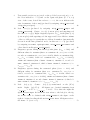
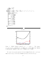
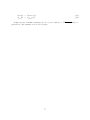
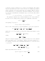
This file is read by the plotting program epe3ak31.u and give global time evolution of the
simulation from the point of view of the MHD module (see Fig. (4)). An example of the input
file xepe3ak31 datain for the program epe3ak31.u is listed hereafter:
...
ENERGY
0
0
CHANGE TSTART (IF 1 ADD IN THE NEXT LINE NEW TSTART)
CHANGE TEND
(IF 1 ADD IN THE NEXT LINE NEW TEND)
1
1
0
1
1.e-30,1.e-4
MODECH (1-MODES , 2-ENERGY , 3-PARAMETERS 4-MAGNETIC SIGNALS)
IC (1-MAGNETIC , 2-KINETIC , 3-TOTAL)
CHANGE MODE LIST (IF 1 ENTER SEQUENCE OF MODE CHANGE)
CHANGE LIMITS (IF 1 NEW LIMITS ARE ENTERED BY TERMINAL)
1
2
0
1
1.e-30,1.e-4
MODECH (1-MODES , 2-ENERGY , 3-PARAMETERS 4-MAGNETIC SIGNALS)
IC (1-MAGNETIC , 2-KINETIC , 3-TOTAL)
CHANGE MODE LIST (IF 1 ENTER SEQUENCE OF MODE CHANGE)
CHANGE LIMITS (IF 1 NEW LIMITS ARE ENTERED BY TERMINAL)
1
3
0
1
1.e-30,1.e-4
MODECH (1-MODES , 2-ENERGY , 3-PARAMETERS 4-MAGNETIC SIGNALS)
IC (1-MAGNETIC , 2-KINETIC , 3-TOTAL)
CHANGE MODE LIST (IF 1 ENTER SEQUENCE OF MODE CHANGE)
CHANGE LIMITS (IF 1 NEW LIMITS ARE ENTERED BY TERMINAL)
0
exit
...
Note that in the above list only the sequence of input data suited for MODECH=1 have been
shown; different values of MODECH will provide plots of other quantities and will require different
input data.
33
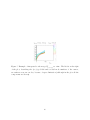
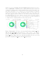
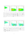
Figure 4: Radially integrated magnetic energy of the perturbed Fourier components
vs. time: the flag (fourth column) in the TMODE PL input file commands the Fourier
components to be plotted. Note that here the result of a simulation in which nout=100.
is shown.
34
After running the program epe3ak31.u, an output file is written which can be used to
produce a time sequence of plots (movie) by the fortran plot energy.f. An example of the
input file xplot energy input for the program plot energy.f is listed hereafter:
...
ENERGY
TMODE_PL
0
pippo.eps
1, 321, 10
3
0.
1.e-32, 0.
161
161
5
ips 0: no PostScript file, 1: PS file, 2: EPS, name follows (30 char.)
ifirst_step,itot,increm (output time steps)
1=magnetic energy, 2=kinetic energy, 3=magnetic + kinetic energy
time_max (if 0, take time_max from stop_run file)
y_en_min, y_en_max
ipl0 first plot
ipl1 last plot
...
The above input data example contains: the name of the input data files (ENERGY,
TMODE PL). ips is a flag for producing a PostScript output, followed by the name of such
a file (pippo.eps). ifirst step,itot are the first and last output time steps which will
be read and available for plotting, respectively; frames will be produced every increm
steps.
An output time step corresponds to NPRI simulation time steps, i.e.
ulation time ∆toutput,MHD = DT*NPRI (in Alfv´en time units).
to a sim-
time max is the limit of
the abscissa (in Alfv´en time units, if time max=0., the maximum of the abscissa will be
calculated automatically by the input parameters of the run).
Note that for a simula-
tion with DT=0.02, NCYCLE=160, NSUBCY=3, NPRI=30, NOUT=20 we get a total number of
time steps equal to NCYCLE*NSUBCY*NOUT+1=9601 (t=0 is also counted) corresponding to
time max=DT*NCYCLE*NSUBCY*NOUT=192.0, and (NCYCLE*NSUBCY*NOUT/NPRI)+1=321 output
times. y en min, y en max are the limits of the ordinate (if y en min=0. and/or y en max=0.,
these limits are computed from the data). ipl0 and ipl1 are the first and last time steps at
which graphical frames will be produced (in the above example, only the frame number “161”
will be produced, corresponding to the normalized time tωA0 = (161 − 1)*DT*NPRI = 96.).
The parameter “5” is a parameter required by the plotting routines (HIGZ from CERN) which
identify the graphic window.
In Fig. (5) an example of this plot is shown:
35
Figure 5: Example of integrated total energy Wtot−m,n vs. time. The labels on the right
of the plot, describing the (m, n) poloidal and toroidal mode numbers of the curves,
are written every two modes, because of space limitation (although in the plot all the
components are shown).
36
4.3
Output file CTBO
The CTBO file contains radial profile data of MHD quantities, at the end of the simulation (or
each NCYCLE*NSUBCY times, if fortran is modified accordingly).
...
WRITE(CHCTBO,1900) ETA,VISC,DT,TIME,REAL(NR),REAL(LM),REAL(IRMODE)
WRITE(CHCTBO,1900) (RM(L),RN(L),L=1,LM)
WRITE(CHCTBO,1900) (R(I),I=1,NR)
1900 FORMAT(6(E20.13,’,’))
c...
WRITE(CHCTBO,1950) ((PSI(I,L),I=1,NP),L=1,LM)
WRITE(CHCTBO,1950) ((PHI(I,L),I=1,NR),L=1,LM)
CGV
WRITE(CHCTBO,1950) ((CUR(I,L),I=1,NR),L=1,LM)
WRITE(CHCTBO,1950) (( W(I,L),I=1,NR),L=1,LM)
CGVKIN..
WRITE(CHCTBO,1950) ((PREK(I,L),I=1,NR),L=1,LM)
CGVKIN..
CGV
1950 FORMAT(3(’(’,E20.13,’,’,E20.13,’),’))
...
The variable IRMODE is an obsolete parameter, included only for compatibility with old
outputs. This output file is read by the plotting program profilk.u and gives the radial profile
for each Fourier poloidal component of the various MHD variables (the poloidal magnetic flux
function PSI ≡ ψm,n (r), the scalar potential PHI ≡ φm,n (r), the toroidal component of the
current CUR ≡ jm,n (r) ≡ −(4∗ ψ)m,n , the toroidal component of the vorticity W ≡ wm,n (r) ≡
(∇2⊥ φ)m,n , and term proportional to the divergence of the energetic particle stress tensor which
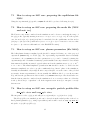
enters in the vorticity equation PREKm,n (r), computed at the time t=TIME, see Fig. (6)). An
example of the input file xprofilk datain for the program profilk.u is listed hereafter:
...
0
0
title
CTBO
1
1
0.,1.,,,
1-PSI 2-W
3-PHI 4-J 5-Q 6-PREK 7-NEW TIME 8-BLANK PLOT
L (mode index) (if l<0, it plots from abs(l) to lm;
do not enter min,max)
X-MIN,X-MAX,Y-MIN,Y-MAX (if commas, it takes computed values)
1
2
0.,1.,,,
1-PSI 2-W
3-PHI 4-J 5-Q 6-PREK 7-NEW TIME 8-BLANK PLOT
L(M,N) (if l<0, it plots from abs(l) to lm; do not enter min,max)
X-MIN,X-MAX,Y-MIN,Y-MAX (if commas, it takes computed values)
8
1-PSI 2-W
1
-3
1-PSI 2-W
3-PHI 4-J 5-Q 6-PREK 7-NEW TIME 8-BLANK PLOT
L(M,N) (if l<0, it plots from abs(l) to lm; do not enter min,max)
8
1-PSI 2-W
3-PHI 4-J 5-Q 6-PREK 7-NEW TIME 8-BLANK PLOT
3-PHI 4-J 5-Q 6-PREK 7-NEW TIME 8-BLANK PLOT
37
3
-3
1-PSI 2-W
3-PHI 4-J 5-Q 6-PREK 7-NEW TIME 8-BLANK PLOT
L(M,N) (if l<0, it plots from abs(l) to lm; do not enter min,max)
8
1-PSI 2-W
6
-3
1-PSI 2-W
3-PHI 4-J 5-Q 6-PREK 7-NEW TIME 8-BLANK PLOT
L(M,N) (if l<0, it plots from abs(l) to lm; do not enter min,max)
8
1-PSI 2-W
2
-1
1-PSI 2-W
3-PHI 4-J 5-Q 6-PREK 7-NEW TIME 8-BLANK PLOT
L(M,N) (if l<0, it plots from abs(l) to lm; do not enter min,max)
8
1-PSI 2-W
4
-1
1-PSI 2-W
3-PHI 4-J 5-Q 6-PREK 7-NEW TIME 8-BLANK PLOT
L(M,N) (if l<0, it plots from abs(l) to lm; do not enter min,max)
7
1-PSI 2-W
3-PHI 4-J 5-Q 6-PREK 7-NEW TIME 8-BLANK PLOT
3-PHI 4-J 5-Q 6-PREK 7-NEW TIME 8-BLANK PLOT
3-PHI 4-J 5-Q 6-PREK 7-NEW TIME 8-BLANK PLOT
3-PHI 4-J 5-Q 6-PREK 7-NEW TIME 8-BLANK PLOT
...
38
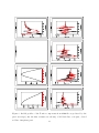
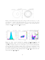
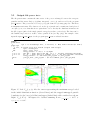
Figure 6: Radial profiles of the Fourier components from CTBO file as produced by the
previous script (only the first 8 frames are shown): solid black line: real part, dotted
red line: imaginary part.
39
5
Output files: produced by the gyrokinetic module
5.1
Output file OUTDNT
This file contains the time series of the radial profiles of energetic particle density DNTOT (normalized energetic particle density), perpendicular PPERP and parallel PPARA energetic particle
pressure. The gyrokinetic module produces an output on the file OUTDNT every NWRITE time
steps (in analogy with the MHD module, with NWRITE taking the place of NPRI), thus the
output time step is given by ∆toutput,GK = DT*NWRITE (in Alfv´en time units).
...
WRITE(43,*)ISTEP0,TIMKIN,DENOUT
IF(ISTEP0.EQ.0)THEN
WRITE(43,*)ASPECT
WRITE(43,*)USPS00
write(43,*)’ 0’
WRITE(43,*)NERRE,LMEQ
DO IR=0,NERRE
WRITE(43,*)RLOW(IR)
ENDDO
c
DO IR=0,NERRE
DO LMODE=1,LMEQ
WRITE(43,*)PSIEQ(LMODE,IR)
ENDDO
ENDDO
c
DO LMODE=1,LMEQ
WRITE(43,*)MMODE(LMODE)
ENDDO
ENDIF
c...
DO 1 JJER=0,NLR
WRITE(43,*)DNTOT(JJER),ANTOT,PPERP(JJER),PPARA(JJER)
1 CONTINUE
...
ISTEP0 is the current time step index, TIMKIN is the (normalized) current time,
DENOUT=0.0, USPS00= (ψ0,0 (r)|max )−1 , ASPECT is the aspect ratio R0 /a, NERRE=NR-1, RLOW
is the radial coordinate of the mesh used by the MHD module, PSIEQ are the radial profiles
of the LMEQ equilibrium Fourier components of ψ, MMODE(l) = m(l), ANTOT is an obsolete
quantity. This file is used to produce movies of density, βH and αH (local drive) energetic
particle profiles evolution (see Fig. (7)) using the plot program plot density.f. An example
of the input file xplot density input for the program plot density.f is listed hereafter:
40
...
ENERGY
APWRITE
OUTDNT
0
pippo.eps
1, 321, 10
0
161
161
0. 0.
0. 1.20
0. 0.011
-1.5 1.5
5
ips 0: no PostScript file, 1: PS file, 2: EPS, name follows (30 char.)
ifirst_step,itot,increm (output time steps)
1=plot n_H-density, 2= beta_H, 3= alpha_H, 0= all
ipl0 first plot
ipl1 last plot
xldmin, xldmax (x axis, if 0.,0. use automatic values)
aldmin, aldmax (density, if 0.,0. use automatic values)
albmin, albmax (beta_H, if 0.,0. use automatic values)
alamin, alamax (alpha_H, if 0.,0. use automatic values)
...
In
the
above
example,
which
refers
NCYCLE=160, NSUBCY=3, NWRITE=30, NOUT=20,
to
we
a
get
simulation
a
total
with
number
DT=0.02,
of
time
steps equal to NCYCLE*NSUBCY*NOUT+1=9601 (t=0 is also counted) corresponding to
time max=DT*NCYCLE*NSUBCY*NOUT=192.0,
and
(NCYCLE*NSUBCY*NOUT/NWRITE)+1=321
output times. Only the plots corresponding to the output time step ipl0 = ipl1 = 161
will be produced, that is at the normalized time tωA0 = (161 − 1)*DT*NWRITE = 96. The
parameter “5” in the last line of the file xplot density input is a parameter required by the
plotting routines (HIGZ from CERN) which identifies the graphic window.
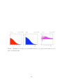
The plotted quantities are given in terms of the quantities written in the file OUTDNT by:
• nH (r)/nH0 = DNTOT(r)/(2π∆r) where ∆r = 1/NLR;
• βH (r) = 2 × EMHSMI × VTHSVA2 × ENHSNI × [2 × PPERP(r)/3 + PPARA(r)/3]/(2π∆r)
• αH = −R0 /a × q 2 (r)dβH /dr.
41
Figure 7: Example for density, βH (red dashed curve is β⊥,H , green dotted curve is βk,H )
and αH radial profiles.
42
5.2
Output file TESTWRIK
This file contains the time history of the test particles, and it is used to plot test particle
quantities (see Fig. (8)) using the plot program plot field.f. The quantities written are:
rtest , θtest , ϕtest , utest , wtest , ∆test (see Sect. (9.4)). The following excerpt shows the write statements in the file TESTWRIK:
...
IF(ISTEP0.EQ.0)THEN
C----------------------------------------------------------------------WRITE(29,*) ASPECT
WRITE(29,*) NPTEST
DO 335 I=1,NPTEST
WRITE(29,*) ITEST(I)
IF(ITEST(I).EQ.0)THEN
WRITE(29,*) ER0T(I),TH0T(I),PH0T(I),AM0T(I),U0T(I)
ELSE
WRITE(29,*) LTEST(I)
ENDIF
335 CONTINUE
C----------------------------------------------------------------------ENDIF
C----------------------------------------------------------------------C
WRITE THE TIME STEP AND THE QUANTITY DENOUT INTO FILE 29
C----------------------------------------------------------------------WRITE(29,*)ISTEP0,TIMKIN,DENOUT
C----------------------------------------------------------------------C
WRITE THE RELEVANT DATA INTO FILE 29
C----------------------------------------------------------------------DO 1 L=1,NPTEST
WRITE(29,*)ERTEST(L),THTEST(L),PHTEST(L),UTEST(L)
WRITE(29,*)WTEST(L),DTEST(L)
1 CONTINUE
...
Units and normalizations are:
• ERTEST ≡ rtest normalized to minor radius a;
• THTEST ≡ θtest in radiants;
• PHTEST ≡ ϕtest in radiants;
• UTEST ≡ utest = vpar /vH (ψ = 0), with vH (ψ = 0) =
p
TH (ψ = 0)/mH . TH (ψ = 0) is:
1. the temperature at ψ = 0 for Maxwellian distribution function (idistr=1);
2. the birth energy E0 for the slowing down distribution function (idistr=2);
3. the perpendicular temperature at ψ = 0 for the bi-Maxwellian distribution function
(idistr=3);
• AM0T ≡ µ ∗ ΩH (ψ = 0)/TH (ψ = 0), with µ being the magnetic moment and ΩH (ψ = 0)
the Larmor frequency of the energetic particle at ψ = 0;
43
Note that here ψ = 0 defines the magnetic axis.
44
5.3
Outputs file PHIWRITE and APWRITE
These files contain the time sequences of the radial profiles of the Fourier components of
φm,n (r) and ψm,n (r), respectively, on the radial grid of the gyrokinetic module and normalized
according to the normalizations used therein. The files are in unformatted format. The
following excerpts show the write statements in the file PHIWRITE (unit=63) and APWRITE
(unit=64):
...
WRITE(63)ISTEP0,TIMKIN
IF(ISTEP0.EQ.0)THEN
WRITE(63)NLR,NTH,NPH
WRITE(63)(ERG(JER),JER=0,NLR)
WRITE(63)LMPERT
write(63) (mmode(im),nmode(im),im=1,lmpert)
ENDIF
write(63) ((phmhdg(im,jer),im=1,lmpert),jer=0,nlr)
...
...
...
...
write(64) ((apmhdg(im,jer)+psieqg(im,jer),im=1,lmpert)
&
,jer=0,nlr)
...
...
Note that the file APWRITE contains the ψm,n (r) components (perturbation part apmhdg
plus equilibrium part psieqg) and the file PHIWRITE contains φm,n (r) (perturbation part
phmhdg, equilibrium part assumed to be zero). ERG is radial coordinate of the mesh used
by the the gyrokinetic module, LMPERT=LM. Those files are used to produce a sequence of
frames of a series of quantities (only the ones produced for φm,n (r) are shown in the following
Figs. (8), (10)), using the plotting program plot field.f. The plots are the following: contour plot of φ(r, θ, ϕ = phiplot), φ(r, θ, ϕ = ϕi (t)) with superimposed the trajectory of the
ith test particle, trajectories of the ith test particle ri = ri (t), θi = θi (t), ϕi = ϕi (t), ui = ui (t)
(see Fig. (8)), trajectory of the ith test particle in the poloidal (R, Z) and equatorial (X,Y)
plane (see Fig. (9)), radial profiles of the φm,n Fourier components, contour plot of φm,n (r) in
the plane (r, m) with superimposed the curve m = nq(r), contour plot of the power spectrum
P (r, ω) in the plane (r, ω) with superimposed the lower and upper Alfv´en continua for the
toroidal gap, ξr (r) (radial component of the displacement) and δTe (r) (electron temperature
fluctuation) assuming incompressible perturbations. The power spectrum P (r, ω) is defined
as:
P (r, ω) = Σm,n Pm,n (r, ω) ∝ Σm,n |φm,n (r, ω)|2 + |φm,n (r, −ω)|2 .
45
(10)
An example of the input file xplot field input for the program plot field.f is listed
hereafter:
...
ENERGY
PHIWRITE
APWRITE
TESTWRIK
Te_vs_erg_DIII_D_1_interp.txt
0
ips 0: no PostScript file, 1: PS file, 2: EPS, name follows (30 char.)
pippo.eps
1, 321, 10 ifirst_step,itot,increm (output time steps)
1
1: phi, 2: psi
0.
phiplot: toroidal angle for (r,theta) plot only
1
ipl0 first plot
321
ipl1 last plot
0,0
l-min, l-max Fourier components used (0,0 all)
1
iflag_rtheta, 1 plot in (r,theta,phiplot) plane (ph/ap_xxxx.gif)
0
iflag_test, superimposes to (r,theta,phtest) plot the
i-th test particle (i=iflag_test)
0
iflag_trajectory, plot particle trajectory in
(rtest,thtest,phtest,utest) space
(trajec_[i]_xxxx.gif, trajRZ_[i]_xxxx.gif, trajXY_[i]_xxxx.gif)
0
iflag_fourier_comp: 1 plot fourier component profiles
0
iflag_contour: 1 2D plot of Fourier components (mn_ph/ap_xxxx.gif),
2 contour plot (mn_C_ph/ap_xxxx.gif),
0 do both
0
iflag_power_spectrum: 1 power power spectrum of field in the
plane (omega,r)
576.
time window for Fourier transform
0. 0.
r0, r1 (min, max in r,
if 0. 0. use max available interval)
0. 0.25
w0, w1 (min, max in omega, if 0. 0. use max available interval)
1
ihann- Hanning function 0: off, 1: on
3
ibuffer (1: no buffer, n>1: zero buffer n-1 times)
0 0.001 ilog, fac_zmin (color scale, 0: linear, 1: log, min value plotted)
505 505 ndivx, ndivy for power spectrum plot axes
.true.
logic_fill (false: only contour, true: fill)
0
call cerca_massimi for plotta_max (0: no, 1: yes)
0
iflag_deltate, synthetic diagnostic Delta_Te
-0.1 0.1 csi0, csi1
(min, max in csi,
if 0. 0. use max available interval)
-50. 50.0 deltate0, deltate1 (min, max in deltate,
if 0. 0. use max available interval)
5
...
Note that the previous input file will produce a sequence of plots starting from tωA0 = 0. to
tωA0 = 96.; only a single frame will be shown in the following Figures 8, 9, 10. iflag test can
vary from “0” (no test particle plots) to NPTEST (producing plots for the i-th test particle).
iflag trajectory=1 will produce, in addition, the trajectories of the selected test particle
(rtest (t), θtest (t), ϕtest (t), utest (t)).
The input file Te vs erg DIII D 1 interp.txt contains the vectors r, Te (r) on the NRL
mesh for synthetic diagnostics purposes (to be produced by the user).
Note that for producing the power spectrum in the plane (r, ω) one has to choose the time
window used in the FFT (twindow = TFFT ωA0 ); the minimum frequency ωmin resolved is
46
given by: ωmin /ωA0 = 2π/twindow, whereas the maximum frequency is given by ωmax /ωA0 =
π/∆t = π/(NWRITE*DT). To minimize the effect of having a finite time sequence, the data can
be multiplied by a Hanning function, which essentially is a function picked at the middle of the
time sequence and which goes to zero toward the edge. To increase the number of points in the
frequency direction (but not the content of information!) a buffer of zeros can be added to the
time sequence using the parameter ibuffer. Note also that the plotting routines interpolate
the resulting FFT function in order to draw the contour plot curves: care should be taken in
choosing the twindow parameter in order to resolve a specific mode (see Fig. 11 and Fig. 12
to compare the effect of different parameters on the produced spectra).
Figure 8: Frames number “161” (tωA0 = 96.) as produced by the program plot field.f
using the xplot field input data shown above.
Left: φ(r, θ, ϕ = 0).
Centre:
φ(r, θ, ϕ) and superimposed the position of the first test particle (produced by assigning iflag test=1). Right: trajectories of the first test particle (rtest , θtest , ϕtest , utest )
(produced by assigning iflag test=1 and iflag trajectory=1).
47
Figure 9: Test particle trajectory projected on the poloidal cross section (ϕ = 0., the
cross indicates r = 0) and on the equatorial plane (Z = 0, top view of the torus, dotted
line refers to r = 0, the cross indicates the axis of symmetry of the torus) (produced by
assigning iflag test=1 and iflag trajectory=1).
Figure 10:
Left:
φm,n (r) (produced by assigning iflag fourier comp=1 and
iflag contour=0). Centre: φm,n (r) (contour plot) and superimposed the curve m =
nq(r). Right: frequency spectra of φm,n in the plane (r, ω) (contour plot) with superimposed the upper and lower Alfv´en continua of the toroidal gap for a particular toroidal
mode number (automatically chosen from the first perturbed mode, in this case n = 2)
(produced by assigning itot=961, ipl0=ipl1=481, iflag power spectrum=1 and other
data from file xplot field input).
48
Figure 11: Frequency spectra during the linear growth phase (tωA0 = 144.) and different values for twindow (first row: twindow=48., ωmin /ωA0 ' 0.131, second row:
twindow=96., ωmin /ωA0 ' 0.0654, third row: twindow=144., ωmin /ωA0 ' 0.0436,
forth row: twindow=192., ωmin /ωA0 ' 0.0327), ihann and ibuffer (first column:
ihann=0, ibuffer=1, second column: ihann=1, ibuffer=1, third column: ihann=1,
ibuffer=3, i.e. ωmin,plot = ωmin /3).
49
Figure 12: Frequency spectra during the saturated phase (tωA0 = 432.) and different values for twindow (first row: twindow=72., ωmin /ωA0 ' 0.0873, second row:
twindow=144., ωmin /ωA0 ' 0.0436, third row: twindow=288., ωmin /ωA0 ' 0.0218),
ihann and ibuffer (first column: ihann=0, ibuffer=1, second column: ihann=1,
ibuffer=1, third column: ihann=1, ibuffer=3, i.e. ωmin,plot = ωmin /3).
50
5.4
Output file deltaf.data (deltaf ealfa.data)
The file deltaf.data contains the time series of the energetic particle distribution function
fH (r, µ, u) (thus, integrated over θ, ϕ), and is read by the program plot deltaf.f (see
Sect. 6 for the details on the distribution function). The distribution function is stored on
a (r, µ, u) grid defined for plotting purposes. More precisely, the number of energetic particles
NH (ri , µj , uk ) in the volume centered at (ri , µj , uk ) is given by:
NH (ri , µj , uk ) = nH (0)a3 fH (ri , µj , uk )dri dµj duk .
The file is in unformatted format. The file deltaf ealfa.data contains the same data but
on a (E, α) mesh instead of (µ, u). The data stored on the (µ, u) mesh can be transformed
and plotted on a (E, α) one; note that this is not equivalent to store directly the distribution
function in the (E, α) space (indeed, the single particle energy dependence on θ is lost). The
data can be also summed up between to radii to reduce particle noise (see Fig. (13)). The
plotting routines allow to subtract to the current fH (r, µ, u, t) the value of fH (r, µ, u, t = trelax ),
where t = trelax is a specific time (thus, the δfH (r, µ, u) is plotted, see Fig. (14))). An example
of the input file xplot deltaf input for the program plot deltaf.f is listed hereafter:
...
deltaf.data
0
ips 0: no PostScript file, 1: PS file, 2: EPS, name follows (30 char.)
pippo.eps
1, 321, 1 ifirst_step,itot,increm (output time steps)
1
ipl0 - first plot
211
ipl1 - last plot
1
iflag - 1:plot deltaf, 2:plot deltaf_ealfa
0
iflag_df - 0: plot f, 1: f_t-f_t_relax
1
iflag_versus - 1: mu,u, 2: E,alpha (only if iflag=1)
0.00 0.00
am0 am1 - (min, max in mu (E) if 0. 0. use max available interval)
0.00 0.00
u0, u1 - (min, max in u (alpha) if 0. 0. use max available interval)
1
iflag_contrai - 1: sum from jer0_pl_min to jer0_pl_max
24 40
jer0_pl_min, jer0_pl_max - (if not summed, plot jer0_pl_min)
0
iflag_relax - 1: reset timkin_relax
120.
timkin_relax_new
0
iflag_renorm - 1: renormalize f_t_relax to n_H(r,t_relax)
and f_t to n_H(r,t) (only if iflag_df=1)
1
iflag_filtro - 1: plot of sedentary and displaced particles df
(only if iflag_df=1)
5
...
51
Figure 13: Left: fH (r, µ, u). Centre: fH (r, µ, u) transformed on the (E, α) mesh. Right:
fH (r, E, α). All figures are obtained summing from rjer0
pl min
= 0.375 to rjer0
pl max
=
0.625. Note that the input file xplot deltaf input shown in the text refers to the
left plot; the figure in the centre is obtained with iflag versus=2; the figure on the
right is obtained reading the file deltaf ealfa.data. All figures refer to the frame “1”
(tωA0 = 0.).
Figure 14: Left: δfH (r, µ, u). Centre: δfH (r, µ, u) transformed on the (E, α) mesh.
Right: δfH (r, E, α). All figures are obtained summing from rjer0
rjer0
pl max
= 0.625.
The relaxed time is trelax = 120.
pl min
= 0.375 to
With respect to the in-
put file xplot deltaf input shown in the text, the figures are obtained by assigning
iflag df=1. All figures refer to the frame “211” (tωA0 = 126.).
52
5.5
Output file power.data
The file power.data contains the time series of the power exchanged between the energetic
particles and the waves PH (r, µ, u) (thus, integrated over θ, ϕ), and is read by the program
plot power.f. The power is stored on a (r, µ, u) grid defined for plotting purposes. The file is
in unformatted format. The data stored on the (µ, u) mesh can be transformed and plotted
on a (E, α) one; note that this is not equivalent to store directly the distribution function in
the (E, α) space (indeed, the single particle energy dependence on θ is lost). The data can be
also summed up between to radii to reduce particle noise (see Fig. (15)). An example of the
input file xplot power input for the program plot power.f is listed hereafter:
...
ENERGY
power.data
0
ips 0: no PostScript file, 1: PS file, 2: EPS, name follows (30 char.)
pippo.eps
1, 321, 10 ifirst_step,itot,increm (output time steps)
161
ipl0 - first plot
161
ipl1 - last plot
2
iflag_versus - 1: mu,u, 2: E,alpha
0.00 0.00
am0 am1 - (min, max in mu (E) if 0. 0. use max available interval)
0.00 0.00
u0, u1 - (min, max in u (alpha) if 0. 0. use max available interval)
1
iflag_contrai - 1: sum from jer0_pl_min to jer0_pl_max
24 40
jer0_pl_min, jer0_pl_max - (if not summed, plot jer0_pl_min)
5
...
Figure 15: Left: PH (r, µ, u). Also the curves representing the maximum energy loaded
in the initial distribution function (dotted lines) and the trapped-untrapped particle
boundaries for the lower (solid line) and upper (dashed line) radii considered are shown.
Right: PH (r, E, α). All figures are obtained summing from rjer0
rjer0
pl max
= 0.625.
53
pl min
= 0.375 to
6
Energetic particle distribution functions
HMGC considers at present three different initial energetic particle equilibrium distribution functions fEQ , namely anisotropic Maxwellian (idistr=1), anisotropic slowing down (idistr=2),
and bi-Maxwellian (idistr=3). Their expressions are listed hereafter.
6.1
Maxwellian distribution function (idistr=1)
The Maxwellian energetic particle equilibrium distribution function fEQ,Maxw is defined as
follows:
nH0 mH 3/2 ˆ
fEQ,Maxw ,
3/2
2π
T
fEQ,Maxw =
(11)
H0
n
ˆ (ψ)
Θ(α, α0 , ∆)e−E/TH (ψ) ,
3/2
τ (ψ)
1
mH u2 + µΩcH ,
2
h
i
cos α−cos α0 2
exp
−
∆
4
√
1−cos
α
α0 ,
0
∆ π erf
+ erf 1+cos
∆
∆
u
p
,
2E/mH
µΩcH
,
E
nH0 n
ˆ (ψ) ,
fˆEQ,Maxw =
E =
Θ(α, α0 , ∆) ≡
cos α ≡
sin2 α ≡
nH (ψ) =
TH (ψ) = TH0 τ (ψ) ,
(12)
(13)
(14)
(15)
(16)
(17)
(18)
with E the energy, nH (ψ) the radial density profile, TH (ψ) the temperature, u the parallel
(to the equilibrium magnetic field) velocity, µ the conserved magnetic moment, α the pitch
angle of the energetic particles and Θ(α) represents the anisotropy of the distribution function.
nH0 = nH (r = 0), TH0 = TH (r = 0), ΩcH = eH B/(mH c) with eH , mH the charge and the
mass of the energetic particle, respectively, and B the (local) equilibrium magnetic field. The
parameters entering in the anisotropy term Θ have the following meaning: α0 is the injection
angle (e.g., in the case of beams) and ∆ is the width of the beam around cos(α0 ). In the code,
the parallel velocity is normalized to the on-axis energetic particle thermal velocity u
ˆ ≡ u/vth0 ,
p
ˆ ≡ µΩcH0 /TH0 , with
with vth0 = TH0 /mH , and the magnetic moment is normalized to µ
ΩcH0 = eH B0 /(mH c).
From the slowing down definition of the distribution function, it follows that:
Z
π
sin αdαΘ(α) = 2 ,
0
54
(19)
Relevant limits are:
∆ −→ ∞ = Θ(α) = 1
∆ −→ 0 = Θ(α) = 2δ(cos α − cos α0 )
(20)
(21)
The definition of the pressure tensor is:
Z
pk =
d3 v 2F E cos2 α ,
(22)
Z
d3 v F E sin2 α ,
Z
pk + 2p⊥
2
=
d3 v F E ,
3
3
p⊥ =
p =
(23)
(24)
where F is the distribution function. From the normalization condition (19) it follows:
3
pΛ ,
2 k
3
pΛ⊥ ,
=
Z2
pk =
(25)
p⊥
(26)
π
dα sin α cos2 α Θ(α) ,
Λk =
(27)
0
Λ⊥ =
1
2
Z
π
dα sin3 α Θ(α) ,
(28)
0
1
Λ⊥ + Λk = 1 .
2
(29)
Then
p⊥ /pk =
1
1
− .
Λk 2
(30)
If the ratio p⊥ /pk is provided experimentally, the corresponding value for ∆ can be obtained
implicitly from Eq. (30) (see Fig. (16)). The explicit expression for Λk is:
Z
Λk =
π
dα sin α cos2 α Θ(α) =
(31)
0
2∆2 π −1/2
α0 ×
erf
+ erf 1+cos
∆
" " (
# #)
1 − cos α0 2
1 − cos α0
1 + cos α0 2
1 + cos α0
exp −
+
exp −
.
∆
∆
∆
∆
= 2 cos2 α0 + ∆2 −
1−cos α0
∆
55
Pperpsuppar[Delta]
cosalfa_0=0.68128
Figure 16: pperp /ppar vs. ∆.
6.2
Slowing down distribution function (idistr=2)
The slowing down energetic particle equilibrium distribution function fEQ,sd is defined as
follows:
fEQ,sd =
fˆEQ,sd =
nH0
3/2
Ecrit,0
3 mH 3/2 ˆ
fEQ,sd ,
4π
2
(32)
n
ˆ (ψ)
Θ(α, α0 , ∆)
h
i h
i,
3/2
3/2
τ (ψ)
(E/Ecrit ) + 1 ln 1 + (E0 /Ecrit )3/2
(33)
In this case the quantity τ is given by τ ≡ Ecrit (ψ)/Ecrit,0 with Ecrit being the critical
energy (see Stix [8]):
3/2
Ecrit (ψ)[MeV] = 14.8Te (ψ)[MeV]
AH X ni (ψ)Zi2
ne (ψ)
Ai
!2/3
,
(34)
i
with AH the mass number of the energetic ions, Ai and Zi the mass number and electric charge
of the bulk ions (plus impurity, eventually) and Te the electron temperature in MeV, ne and
ni the electron and bulk ion densities. E0 is the birth energy of the energetic particles and
Ecrit,0 = Ecrit (0). In the code, the parallel velocity is normalized, in this case, to the energetic
p
particle birth energy velocity u
ˆ ≡ u/vth0 , with vth0 = E0 /mH .
6.3
Bi-Maxwellian distribution function (idistr=3)
The Bi-Maxwellian energetic particle equilibrium distribution function fEQ,bi−Maxw is defined
as follows:
fEQ,bi−Maxw =
fˆEQ,bi−Maxw =
nH0 mH 3/2 ˆ
fEQ,bi−Maxw ,
(35)
3/2
T⊥H0 2π
n
ˆ (ψ)
T⊥H0 1/2
mH u2
µΩcH
exp −
+
. (36)
2TkH0 τk (ψ) T⊥H0 τ⊥ (ψ)
τ⊥ (ψ)τk (ψ)1/2 TkH0
56
T⊥H (ψ) = T⊥H0 τ⊥ (ψ) ,
(37)
TkH (ψ) = TkH0 τk (ψ) .
(38)
In this case the normalized quantities are u
ˆ ≡ u/vth0 , with vth0 =
µΩcH0 /T⊥H0 . The quantity σ0 is σ0 ≡ T⊥H0 /TkH0 .
57
p
T⊥H0 /mH and µ
ˆ≡
7
How to setup an HMGC run
In this section we will give indications on how to set up a specific run of HMGC: we will refer to
a DIII-D discharge (#122117) analyzed in Ref. [7].
W.W. Heidbrink provide us a set of radial profiles for the following quantities (t = 0.414
s) of the DIII-D discharge (see Table (10) and Fig. (17)).
ne (r)
Electron density (cm-3)
ni (r)
(Thermal) deuterium density (cm-3)
nimp (r)
Impurity density (carbon) (cm-3)
nH (r)
Beam-ion density (cm-3) [Note that this transp value is reduced by
fast-ion transport]
Te (r)
Electron temperature (eV)
βH (r)
Beam beta toroidal (dimensionless) [Note that this transp value is
reduced by fast-ion transport]
ωϕ (r)
Toroidal angular velocity (rad/s)
q(r)
safety factor
Table 10: Experimental radial profiles provided by DIII-D team.
The quantity βH (r) will not be used as an input data, but only to compare with the
computed βH (r) from the code (this latter quantity will depend, indeed, on the model used
to load the initial distribution function). The quantity ωϕ (r) could be used to compare the
experimental frequency (νexp ) spectra with the ones obtained by the code (νcode ): νexp =
νcode + (n/2π)ωϕ , with n the toroidal mode number.
In Fig.(18) the geometry of the neutral beam is shown. The beam is essentially tangential,
wit injection angle α0 ≡ arccos(Rtan /R0 ) = arccos(1.15m/1.688m) = 47.055 deg. The average
birth energy is E0 = 0.077 MeV (= 2/3 × 0.075 MeV + 1/3 × 0.081 MeV).
From the data profiles provided and from global information a single toroidal mode number
n = 2 simulation can be set up performing the following steps.
58
vlad-GV
1 10
Beam beta toroidal (dimensionless) [Note that this transp value is reduced by fast-ion transport]
vlad-GV
Temperature (eV)
2 10
13
2 10
13
1 10
0.007
3
0.006
1 10
2
8 10
2
6 10
2
4 10
12
5 10
2
2 10
0
0.0
0.2
0.4
0.6
index()/19
0.8
0
0.0
1.0
Toroidal angular velocity (rad/s)
4
vlad-GV
4
4 10
0.005
0.004
0.003
0.002
0.001
0.2
0.4
0.6
index()/19
0.8
1.0
0
0.0
0.2
0.4
0.6
index()/19
11
vlad-GV
10
4
9
4
8
4
7
3 10
3 10
2 10
q
Toroidal angular velocity (rad/s)
vlad-GV
q
4 10
4
6
4
5
3
4
2 10
1 10
5 10
0
0.0
0.008
3
1 10
13
densities (cm-3)
Ion temperature (eV)
Beam beta toroidal
13
3 10
Electron density (cm-3)
Electron temperature (eV)
(Thermal) deuterium density (cm-3)
Impurity density (carbon) (cm-3)
Beam-ion density (cm-3) [Note that this transp value is reduced by3 fast-ion transport]
0.2
0.4
0.6
index()/19
0.8
1.0
3
0.0
0.2
0.4
0.6
index()/19
0.8
1.0
Figure 17: Experimental profiles for the DIII-D shot # 122117.
59
0.8
1.0
Rtan=115 cm
beam
a=60.9 cm
α0
R0=168.8 cm
α0
cosα0=Rtan/R0
Figure 18: Beam geometry.
60
7.1
How to setup an HMGC run: preparing the equilibrium file
EQNEW
Using the experimental q(r) profile, a EQNEW file should be produced following Sect.(2).
7.2
How to setup an HMGC run: preparing the mode file (TMODE
and modi inc)
The Fourier components considered in the simulation can be chosen considering the range of
the q(r) profile, typically starting from mmin = 1 up to mmax ≈ nq(r = 1). For the specific
case, the modes (m, n) = (0, 0), (1, 0) have been included for the equilibrium, and the modes
(1, 2) up to (21, 2) for the perturbation. (mmax = 2 × q(r = 1) = 2 × 10.5385 ≈ 21; note that
4 × (mmax − 1) = 80 is a valid number for the ESSL FFT routine).
7.3
How to setup an HMGC run: plasma parameters (file PARAM)
The bulk plasma density normalized profile should be assigned following one of the proposed
expressions (NPROFI flag, see Table (3)). For representing experimental data it is usually
convenient to choose NPROFI=1; the three parameters α, β, ρa can be obtained by fitting the
experimental profile. Normalized resistivity η and normalized viscosity ν should be chosen such
that numerical stability is assured: typical values used in the simulations are η = 1. × 10−5 ,
ν = 1. × 10−8 . The initial amplitude perturbation AMP should be such to be well below the
saturation amplitude, in order to provide a sufficiently long “linear” phase of the simulation.
Actually, if is initialized only a single Fourier component (the one at the centre of the poloidal
spectrum). A time step DT must be chosen: usually the MHD module loop on a shorter time
step, whereas the gyrokinetic module is called every NSUBCY time steps. One should take care
that the fastest particles considered in the simulations do not cross more than one cell in the
θ and ϕ directions (or “equivalent” cell, if the nogrid version is used) to integrate correctly
their motion.
7.4
How to setup an HMGC run: energetic particle profiles files
den spli.data and temp spli.data
The integration of the r/q(r) profile will give a ψ(r) mesh (see eq. (9) in Sect. (3.8)).
The Ecrit (r)/Ecrit,0 normalized profile can be derived from the radial profiles of the above
listed plasma quantities (e.g., using a spreadsheet) and it will be used as temp exp DIII D 1
file (table of ψ(r),Ecrit (r)/Ecrit,0 ).
61
Similarly, the energetic particle normalized density profile will be derived by the “Beam-ion
density profile” and used as den exp DIII D 1 file (table of ψ(r),nH (r)/nH0 ).
For each of the previous files, the program interp spline.f is called by the execution
script, producing the files den spli.data and temp spli.data.
7.5
How to setup an HMGC run: energetic particle dimensioning
(file grid inc)
The parameters which describe the energetic particle dimensioning have been chosen according
to Table (11).
64
NLR
low n, should be such to resolve the typical radial
width structure of the perturbed mode
NTH
168
usually take 8 poloidal mesh points times mmax
nintphi
2 × (n − 1)
nph su nintphi
4
ippc
2
two particle per cell per each direction (r, θ, ϕ)
nne
672
as obtained by the program calcolo nne.f
NMODOM
27
see Table (5)
NRZ
5
it depends from the Shafranov shift of the equilibrium (see output of the program eqe3aaab.f,
typically NRZ such to include the magnetic axis is
taken).
Table 11: Preparing the grid inc file.
7.6
How to setup an HMGC run: energetic particle parameters
(file KININP)
The energetic particle parameters can be calculated from the experimental data provided,
namely, energetic ion specie (D: AH = 2, ZH = 1), toroidal field BT 0 = 2 T, R0 = 1.688 m,
a = 0.609 m, Carbon impurity, E0 = 0.077 MeV, volume averaged value of ppar /pperp ≈ 1.44
for the beam ions.
62
RHOSA
ρH0 /a
1/2
1/2
−1
0.032863457d0 1.02 × 10⁻¹ AH ZH
E0,MeV BT−10,Tesla a−1
m
1/2
−1/2
vth
9.79 × 10⁸ E0,MeV AH
vA0
2.18 × 10⁸ BT 0,Tesla ×
(Ai ni,1020 ×m−3 + Aimp nimp,1020 ×m−3 )−1/2
VTHSVA
vth /vA0
1/2
−1/2
0.271063836d0 4.491E0,MeV mH
BT−10,Tesla ×
(Ai ni,1020 ×m−3 + Aimp nimp,1020 ×m−3 )1/2
usdelta 0 input
1/∆
2.3256d0
The corresponding value of ∆ has been
chosen in order to match the experimental value of the ratio ppar /pperp ≈
1.44
cosalfa 0 input
cos α0
0.68128d0
e0sec0
E0 /Ecrit,0
4.153850158d0 Ecrit,0 from Eq. (34), evaluated at r = 0
ENHSNI
nH0 /ni0
0.264848976d0 nH0 /(ni + nimp )
EMHSMI
mH /mi
1.d0
IDISTR
2
Rtan /R0 = 1.15m/1.688m
slowing down distribution function
loaded
Table 12: Preparing the KININP file.
63
8
HMGC directories structure
•
~
/HMGC: main root directory:
1.
~
/HMGC/script: directory containing compilation and execution scripts;
(a) xe3 HMGC: execution script of e3 complete.F;
(b) xequil HMGC: execution script of eqe3aaab.u;
(c) xplot HMGC: execution script for post-processing plot programs (e.g.,
epe3ak31, profilk, plot density, plot field, plot deltaf, plot power);
(d) xpsi from rho q exp: execution script of psi from rho q exp.f.
2. ~
/HMGC/sources: directory containing HMGC sources;
(a) eqe3aaab.u: equilibrium module;
(b) e3 complete.F: MHD module;
(c) kin uncomplete.F: GK module;
(d) extr push complete.F: pushing routine of GK module;
(e) extr pressure complete.F: pressure routine of GK module;
(f) commons for HMGC: commr31 input, commr31 uncomplete.F, double;
(g) calcolo nne.f: program to initialize the particles in the (E, α) space;
(h) interp spline.f: spline program to interpolate experimental data on the
HMGC mesh;
(i) nlr interp spline: common for the spline program interp spline.f;
(j) psi from rho q exp.f: program to generate ψ(r) from r, q(r) experimental
data;
(k) upda.f: simple pre-processing program (to produce goofy.f programs from
goofy.u);
(l) upda.ksh: shell script to run upda;
(m) pwr5 version: temporary directory (architecture dependent) for producing
the executable;
(n) makefile: makefile;
3.
~
/HMGC/graphics: directory containing graphics post-processor programs:
(a) epe3ak31.f;
(b) profilk.f;
(c) plot density.f;
(d) plot energy.f;
64
(e) plot field.f;
(f) plot deltaf.f;
(g) plot power.f;
(h) plotta max1.f;
(i) plot equil.f: simple plotting program to compare a computed equilibrium
with experimental data;
(j) GVGRAPH0LIB:
directory
containing
some
graphical
routines
(library
containing
some
graphical
routines
(library
libgvgraph0.a);
(k) GVGRAPH1LIB:
directory
libgvgraph1.a).
•
~
/HMGC INPUTS
1.
~
/HMGC INPUTS/equilibrium: directory containing equilibrium files;
2.
~
/HMGC INPUTS/profiles: directory containing energetic particle experimental
density and temperatures profiles;
•
~
/HMGC RESULTS: directory containing output results:
1.
~
/HMGC RESULTS/caso equil DIII D 1: directory containing a DIII-D equilibrium
test case;
2.
~
/HMGC RESULTS/caso n2 DIII D 1 test 1: directory containing a DIII-D test
case;
65
9
Generalities on HMGC
...
Beginning of excerpt form the Appendices of Ref. [9]. For the references to equations not
resolved please refer to the original paper.
...
9.1
MHD equations
We wish to start the discussion of the general properties of the Alfv´en-wave spectrum using
simple-model equations, the so-called ideal magnetohydrodynamic (MHD) equations, which
in Gaussian units read [10]:
∂%
+ ∇ · (%v)
∂t
dv
%
dt
d P
dt %Γ
1
E+ v×B
c
= 0,
(39)
1
= −∇P + J × B ,
c
(40)
= 0,
(41)
= 0,
(42)
1 ∂B
,
c ∂t
4π
∇×B =
J,
c
∇ · B = 0.
∇×E = −
(43)
(44)
(45)
In the above equations v is the fluid velocity, J is the plasma current, B is the magnetic field,
% is the mass density, P is the scalar pressure of the plasma, Γ is the ratio of the specific heats,
c is the speed of light, and
d
∂
=
+v·∇
dt
∂t
(46)
is the convective derivative.
The ideal MHD equations describe the plasma as a single fluid. In particular, eq. (39)
describes the time evolution of mass (conservation of the total number of particles). Equation (40) describes the time evolution of momentum, showing that the fluid is subject to
inertial, pressure-gradient and magnetic forces. Equation (41) is the equation of state and
generally describes the polytropic evolution of the plasma. It may be combined with the
continuity equation and written as
dP
= −ΓP ∇ · v .
dt
(47)
Equation (42), the so-called ideal Ohm’s law, describes the plasma as a perfectly conducting
fluid (from which the expression “ideal MHD” originates). Note that in the more general case
66
in which plasma resistivity η is considered, eq. (42) is replaced by
1
E + v × B = ηJ .
c
(48)
...
The elliptic operator
∆∗
is given by
∗
2
∆ ψ =R ∇·
∇ψ
R2
∂
=R
∂R
1 ∂ψ
R ∂R
+
∂2ψ
.
∂Z 2
(49)
...
9.2
Order-3 reduced MHD
We introduce, here, a simplified version of the resistive MHD equations, which will be useful
later for the non-linear study of the Alfv´en modes, greatly reducing the complexity of the
problem. We start from the resistive MHD equations (39-45), with the Ohm’s law generalized
by eq. (48).
Since tokamak plasmas are characterized by values of the safety factor q(r) ≈
(rBϕ )/(RBϑ ) ≈ O(1) (Bϕ and Bϑ are, respectively, the toroidal and poloidal component of
the magnetic field) and inverse aspect ratio = a/R0 much lower than unity, MHD equations
can be simplified by expanding in powers of . This procedure has been widely used, since
the first paper of Strauss [11], both for analytical and numerical work. At the leading order
in , O(2 ), and considering the low-β approximation, β ≈ O(2 ), the reduced-MHD equations
describe the plasma in the cylindrical approximation. Toroidal corrections enter the equations
at the next order in the inverse aspect ratio expansion. The derivation of these equations has
been described in detail in ref. [12] and is only briefly reported here.
Following the low-β tokamak ordering, it is possible to write
B⊥
B/B · ∇
v⊥
≈
≈
≈ O() ,
vA
Bϕ
∇⊥
vϕ
∇(RBϕ )
∇ · v⊥
≈
≈
≈ O(2 ) ,
vA
vA /a
Bϕ
∂
vA
≈
.
∂t
R
Here, a cylindrical-coordinate system (R, Z, ϕ) has been used, and the subscript ⊥ denotes
components perpendicular to ∇ϕ. The magnetic field can be written as
B = F0 + F˜ ∇ϕ + R0 ∇ψ × ∇ϕ + O(3 Bϕ ) ,
(50)
where ψ is the poloidal magnetic flux function, F0 = R0 B0 , B0 is the vacuum (toroidal)
magnetic field at R = R0 , and F˜ ≈ O(2 F0 ) is given, at the leading order, by equilibrium
67
corrections. Substituting eq. (50) and Ohm’s law, eq. (48), into Faraday’s law, eq. (43), we
obtain
R0
1
∂ψ
∇ϕ + c ηJ − v × B = −c∇φ + O(4 vA Bϕ ) ,
∂t
c
(51)
where φ is the scalar potential. Taking the cross product by ∇ϕ, eq. (51) can be solved with
respect to v⊥ :
v⊥ = −
cR2
∇φ × ∇ϕ + O(3 vA ) .
R0 B0
(52)
Equation (52) states that, at the lowest order, the perpendicular velocity is given by the E × B
drift. Then, taking the ∇ϕ component of eq. (51), the following equation for the evolution of
the poloidal magnetic flux function is obtained:
cR2
c ∂φ
c2
∂ψ
=−
∇ψ × ∇ϕ · ∇φ −
+ η ∆∗ ψ + O(4 vA Bϕ ) ,
∂t
R0 B0
R0 ∂ϕ
4π
(53)
with the Grad-Shafranov operator ∆∗ defined by eq. (49).
Upon applying the operator ∇ϕ · ∇ × R2 . . . to the momentum equation, eq. (40), the
following equation for the evolution of the scalar potential is obtained:
D
D
2c ∂φ
c ∂φ
%ˆ
%·
−
∇2⊥ φ + ∇ˆ
−
∇φ =
Dt R0 B0 ∂Z
Dt R0 B0 ∂Z
v 2 Bϕ
B0
B0
B · ∇∆∗ ψ −
−
∇ · R2 ∇P × ∇ϕ + O(4 % A2 ) ,
4πc
cR0
a c
where
%ˆ =
R2
%,
R02
(54)
∂
D
=
+ v⊥ · ∇ ,
Dt
∂t
1 ∂
∂
∂2
R
+
.
R ∂R ∂R ∂Z 2
Note that, both in eq. (53) and eq. (54), vϕ and F˜ enter only at the fourth order in . In eq. (54)
∇2⊥ ≡
the dependence on the density gradient has been retained explicitly. With the particular choice
of the mass density %R2 = %ˆR02 = const, and using the definition of v⊥ given in eq. (52), the
continuity equation, eq. (39), is satisfied up to the third order. The pressure equation becomes
vA Bϕ2
DP
= O(4
).
Dt
a
...
9.3
Hybrid MHD-kinetic models
68
(55)
In order to include in this model the effects on an energetic-ion population, we can take
advantage from the fact that the energetic particle density is typically much smaller than the
bulk plasma density. The following ordering can then be adopted:
TH
≈ O(−2 ) ,
Ti
nH
≈ O(3 ) ,
ni
where nH (ni ) and TH (Ti ) are the energetic particle (bulk ion) density and temperature
respectively. Thus, the following ordering for the ratio of the energetic to bulk ion beta
follows:
βH
≈ O() ,
βi
It can be shown [13] that, making use of the above ordering, the MHD momentum equation
is modified by a term which represent the perpendicular component of the divergence of the
energetic-particle stress tensor ΠH (in ref. [13] an alternative, equivalent form in which the
electric current associated to the energetic ions appears, instead of the energetic-particle stress
tensor, is also derived). Thus, the O(3 ) equation for the evolution of the scalar potential is
modified as follows
D
2c ∂φ
D
c ∂φ
2
%ˆ
−
∇⊥ φ + ∇ˆ
%·
−
∇φ =
Dt R0 B0 ∂Z
Dt R0 B0 ∂Z
v 2 Bϕ
B0
B0
−
B · ∇∆∗ ψ −
∇ · R2 (∇P + ∇ · ΠH ) × ∇ϕ + O(4 % A2 ) .
4πc
cR0
a c
(56)
In order to close the set of reduced MHD eqs. (53) and (56), the hot-particle stress-tensor
components can be evaluated by directly calculating the appropriate velocity moment of the
distribution function for the particle population moving in the perturbed fields ψ and φ (see
appendix sect. 9.4).
...
9.4
Hybrid MHD-kinetic code
In this section, we describe the code that solves the O(3 ) reduced MHD model, in the limit
of zero bulk-plasma pressure. In such limit, only eqs. (53) and (56) need to be solved. As
a boundary condition, we take a rigid conducting wall at the plasma edge. The numerical
tool [14, 15, 16] used to solve the O(3 ) model is based on a field solver originating from an
existing O(2 ) code [17]. Such field solver uses toroidal coordinates (r, ϑ, ϕ), finite differences
in the radial direction (r) and Fourier expansion in the poloidal (ϑ) and toroidal (ϕ) directions. The coupled equations for the Fourier components of the magnetic and velocity stream
functions ψ and φ are advanced in time using a semi-implicit algorithm, where all the linear
terms that couple with the cylindrical part of the equilibrium (i.e., the component having
69
poloidal and toroidal mode numbers (m, n) = (0, 0)) are treated implicitly. The non-linear
terms, the terms which arise from the toroidal corrections to the cylindrical approximation
and the contributions of the energetic particles (the term containing ∇ · ΠH in eq. (56)) are
treated explicitly. Moreover, only the Fourier components in a half plane of the (m, n) space
are evolved, the ones that fall in the other half plane being recovered from the reality condition
of the solution:
∗
ψˆ−m,−n (r, t) = ψˆm,n
(r, t) ,
φˆ−m,−n (r, t) = φˆ∗m,n (r, t) .
(57)
The equilibrium configuration used for numerical simulations can be exactly calculated to
the desired order in , starting from the expression for the equilibrium toroidal current
∆∗ ψ eq = −
4π R
J0ϕ ,
c R0
(58)
and expanding ψ eq in powers of ,
ψ eq (r, ϑ) = ψ0eq (r) + ψ1eq (r, ϑ) + O(2 ψ0eq ) .
In the toroidal coordinate system (r, ϑ, ϕ) the Grad-Shafranov operator can be expressed as
1 ∂
∂
1 ∂2
1
∂
sin ϑ ∂
∗
∆ =
r
+ 2 2−
cos ϑ
−
,
r ∂r
∂r
r ∂ϑ
R
∂r
r ∂ϑ
with R = R0 + r cos ϑ. To the leading order, that is in the cylindrical approximation, eq. (58)
is given by
1 d
r dr
yielding
dψ0eq
r
dr
=−
4π
J0ϕ [ψ0eq (r)] ,
c
(59)
dψ0eq
B0 r
=−
,
dr
R0 q(r)
which can be integrated assigning ψ0eq (a) = 0 and q(r), the safety factor in the cylindrical
(O(2 )) approximation (q(r) = rB0ϕ /(R0 B0ϑ )). Equation (59) gives the symmetric (m =
0, n = 0) Fourier component of the poloidal magnetic flux function ψ eq . To the next order in
, eq. (58) yields
1 ∂
r ∂r
∂ψ eq
1 ∂ 2 ψ1eq
1
dψ0eq
r 1 + 2
−
cos
ϑ
=
∂r
r ∂ϑ2
R0
dr
4π eq d
R
− ψ1
J0ϕ .
eq
c
dψ
R0
ψ eq =ψ eq
(60)
0
Equation (60) admits solutions of the form
ψ1eq (r, ϑ) = ψ1eq (r) cos ϑ = ∆(r) cos ϑ
70
dψ0eq
,
dr
(61)
where we have introduced the so-called Shafranov shift ∆. Substituting eq. (61) into eq. (60)
and using the leading order solution of eq. (59), the following equation for the Shafranov shift
∆ is obtained:
" #
2
2
dψ0eq
d∆
1 dψ0eq
1 d
r
−
= 0.
r dr
dr
dr
R0
dr
(62)
Equation (62) can be integrated assigning the radial derivative of the Shafranov shift at the
center ∆0 (0) = 0 (regularity condition) and ∆(a) = 0 (corresponding to ψ eq = 0 on the rigid
conducting wall), to obtain ∆(r). The substitution of ∆(r) into eq. (61) allows us to obtain
the first-order (1, 0) Fourier component of the magnetic flux function ψ eq , thus completing
the equilibrium solution at the desired order. Note that, once fixed r and ϑ, the quantity
∆(r) corresponds to the shift, with respect to the center of the poloidal cross section, of the
geometric center of the magnetic surface labelled by the value ψ eq (r, ϑ). Such a shift causes
shear Alfv´en waves, even when propagating along the magnetic field line, to cross the radial
grid, thus imposing restrictions on the time step of integration [12]. Further restrictions are
imposed by the strength of the explicitly solved terms (as, e.g., in the case of high inverse
aspect ratio equilibria and/or highly non-linear cases).
The term ΠH in eq. (56) is the pressure-tensor of the energetic (hot) ions; it can be
R
expressed in terms of the corresponding distribution function fH (ΠH ≡ mH d3 vvvfH ,
with mH being the energetic-ion mass), to be determined by solving the Vlasov equation
(the collisionless limit of the Boltzmann equation). Since the time scale of the dynamics we
want to analyze is long compared to a cyclotron period, it is convenient [18, 19] to solve
the Vlasov equation in the gyrocenter-coordinate system Z ≡ R, M , U , θ , where R is the
gyrocenter position, M is the magnetic moment, U is the parallel velocity (i.e., the velocity
along the magnetic-field line), and θ is the gyrophase. This corresponds to averaging the
single-particle equations of motion over many cyclotron orbits and allows one to retain the
relevant finite-Larmor-radius effects without resolving the details of the gyromotion. Such
a choice is particularly suited for numerical time integration of the particle motion, as the
numerical-stability constraint on the time-step size turns out to be much less severe than that
we would obtain without adopting the averaging procedure.
The hot-particle pressure tensor assumes the following form, in terms of the gyrocentercoordinate distribution function,
Z
1
ΠH (t, x) = 2
mH
d6 ZDzc →Z F H t, R, M , U ×
ΩH M
ΩH M
2
ˆ
ˆ
I + bb U −
δ x−R ,
(63)
mH
mH
where I is the identity tensor (Iij ≡ δij ), F H t, R, M , U is the energetic-particle distribution
function in gyrocenter coordinates, and Dzc →Z is the Jacobian of the transformation from
71
canonical to gyrocenter coordinates.
The Vlasov equation can be written as
dF H
= 0,
dt
with
(64)
i
d
∂
dZ ∂
≡
+
,
dt
∂t
dt ∂Z i
i
and dZ /dt given by the following equations of motion [14, 20, 21, 22]
ˆ × ∇φ − U b
ˆ × ∇ak +
ˆ + eH b
= Ub
mH ΩH
mH ΩH
ak
M
U
ˆ × ∇ ln B,
+
U+
b
mH
ΩH
mH
dR
dt
dM
dt
dU
dt
= 0,
(65)
ak
1 ˆ
eH
M
b·
U+
∇ak ×∇ ln B +
∇φ +
mH
ΩH
mH
mH
ΩH M ˆ
eH
∇ak ×∇φ −
b · ∇ ln B.
m H ΩH
mH
=
Here, eH and ΩH ≡ eH B/(mH c) are, respectively, the energetic-ion charge and Larmor frequency. The fluctuating potential ak is related to the poloidal magnetic flux function ψ through
the relationship
ak =
eH R0
ψ.
c R
(66)
Note that the magnetic moment M is exactly conserved in this coordinate system and that,
correspondingly, neither F H nor the equations of motion contain any dependence on the gyrophase θ.
The particle-simulation approach to the solution of Vlasov equation, eq. (64), consists in
representing any phase-space function G(t, Z) by its discretized form,
Z
G t, Z ≡
X
d6 Z 0 G t, Z 0 δ Z − Z 0 ≈
∆l G t, Z l δ Z − Z l ,
(67)
l
where ∆l is the volume element around the phase-space marker Z l , and in assuming that
each marker evolves in time according to the gyrocenter equations of motion, eqs. (65). Such
markers can then be interpreted as the phase-space coordinates of a set of Npart “particles”,
and G(t, Z) can be approximated by
Npart
G t, Z ≈
X
∆l (t) G t, Z l (t) δ Z − Z l (t) .
l=1
72
(68)
The time-variation of the volume element ∆l (t) is then given by
d∆l
= ∆l (t)
dt
∂ dZ
i
∂Z dt
i
!
.
(69)
t,Z l (t)
For the purpose of calculating the pressure tensor components, eq.(63), it is convenient to
directly represent the quantity Dzc →Z F H according to its discretized form
Npart
X
Dzc →Z t, Z F H t, Z ≈
wl (t) δ Z − Z l (t) ,
(70)
l=1
with the weight factor wl defined by
wl (t) ≡ ∆l F H t, Z l (t) ,
(71)
∆l ≡ ∆l (t) Dzc →Z t, Z l (t) .
(72)
and
In fact, from eqs.(64), (69), and from the Liouville theorem,
!
i
dZ
∂
∂
Dzc →Z
+
D
=0,
∂t zc →Z ∂Z i
dt
(73)
it is immediate to show that
d∆l
= 0,
dt
(74)
dwl
= 0.
dt
(75)
and
At each time step, the fluctuating electromagnetic potentials are computed at the grid
points of a three-dimensional toroidal domain in terms of the Fourier components yielded
by the field solver. Phase-space coordinates are then evolved in the fluctuating fields, and
the pressure tensor components at the grid points are updated, in order to close the MHD
equations for the next time step.
Field values at each particle position are obtained by trilinear interpolation of the fields at
the vertices of the cell the particle belongs to. The corresponding trilinear weight function is
adopted, after pushing the particles, in order to distribute their contribution to the pressure
tensor components among the vertices of the cell. Phase-space coordinates and weights for
the simulation particles are initially determined in such a way to yield a prescribed (e.g.,
Maxwellian) distribution function. Particle pushing is performed by integrating eqs. (65) by
a second-order Runge-Kutta method, more accurate than the standard O(∆t) Euler method
(O(∆t2 ) is properly retained), although more time consuming. Particles that hit the wall
(r = a) are considered lost and are not re-injected in the plasma.
73
It has been shown [14, 23, 24, 25, 26, 27] that, as far as regimes are considered where the
distribution function can be expected to slightly depart from the equilibrium one, it is worth
limiting the numerical investigation to the evolution of the perturbed part δF H , defined by
the relationship
F H t, R, M , U = F H0 t, R, M , U + δF H t, R, M , U ,
(76)
where F H0 is the lowest-order (“equilibrium”) distribution function.
In terms of δF H , eq.(64) can be written in the form
dδF H
=S,
dt
(77)
with
dF H0
.
dt
Meanwhile, eq.(70) is replaced by the following one,
S≡−
Npart
X
Dzc →Z t, Z δF H t, Z ≈
wl (t) δ Z − Z l (t) ,
(78)
l=1
with
wl (t) ≡ ∆l δF H t, Z l (t) ,
(79)
and
dwl
= ∆l S t, Z l (t) .
(80)
dt
Note that eq.(76) is by no means equivalent to a linearization of the Vlasov equation, since
all non-linear terms are correctly retained. The decomposition of eq.(76) is useful in reducing
numerical noise as long as |δF H | |F H0 |.
In the present paper, when adopting the δF approach, we take F H0 to be Maxwellian
!
2
ΩH M + 12 mH U
F H0 ∝ nH R exp −
,
(81)
TH
where nH R and TH are, respectively, the energetic-particle equilibrium density and (uniform) temperature. The r.h.s. of eq.(77) is then given by
ak
dR
eH M
U
ˆ × ∇ ln B·∇φ+
S t, R, M , U = −F H0
·∇ ln nH +
+
U+
b
dt
TH mH
ΩH
mH
eH U ˆ
b · ∇φ×∇ak .
(82)
TH ΩH mH
We also assume the following model for the energetic-particle equilibrium density:
2 αn r
nH (r) = nH0 exp −
,
L2n
74
(83)
where nH0 is the on-axis density.
...
End of excerpt form the Appendices of Ref. [9].
...
References
[1] Frieman E. and Chen L., 1982 Physics of Fluids 25 502
[2] Lee W., 1987 Journal of Computational Physics 72 243
[3] Shinohara K., et al., 2001 Nuclear Fusion 41 603
[4] Shinohara K., et al., 2002 Nuclear Fusion 42 942
[5] Shinohara K., et al., 2004 Plasma Phys. Contr. Fusion 46 S31–45
[6] G. Vlad, S. Briguglio, G. Fogaccia, and B. Di Martino. Gridless finite-size-particle plasma
simulation. Computer Physics Communication, 134:58–77, 2001.
[7] G. Vlad, S. Briguglio, G. Fogaccia, F. Zonca, W. W. Heidbrink, and M. A. Van Zeeland.
Particle simulations of Alfv´en modes in reversed-shear DIII-D discharges heated by neutral
beams. In 10th IAEA Technical Meeting on Energetic Particles in Magnetic Confinement
Systems, Kloster Seeon 8-10 Oct. 2007, page OT 7, Vienna, Austria, 2007. International
Atomic Energy Agency.
[8] Stix T H 1972 Plasma Phys. 14 367-84
[9] G. Vlad, F. Zonca, and S. Briguglio. Dynamics of Alfv´en waves in tokamaks. Rivista del
Nuovo Cimento, 22(7):1–97, 1999.
[10] J.P. Freidberg, Ideal Magnetohydrodynamics, Plenum Press, New York, 1987.
[11] H.R. Strauss, Phys. Fluids, 20, (1977) 1354.
[12] R. Izzo, D.A. Monticello, W. Park, J. Manickam, H.R. Strauss, R. Grimm, and
K. McGuire, Phys. Fluids, 26, (1983) 2240.
[13] W. Park, S. Parker, H. Biglari, M. Chance, L. Chen, C.Z. Cheng, T.S. Hahm,
W.W. Lee, R. Kulsrud, D. Monticello, L. Sugiyama, and R.B. White, Phys.
Fluids B, 4, (1992) 2033.
75
[14] S. Briguglio, G. Vlad, F. Zonca, and C. Kar. Hybrid magnetohydrodynamic-gyrokinetic
simulation of toroidal Alfv´en modes. Physics of Plasmas, 2:3711–3723, 1995.
[15] G. Vlad, C. Kar, F. Zonca, and F. Romanelli.
of Alfv´en eigenmodes in tokamaks.
Linear and non-linear dynamics
Physics of Plasmas, 2:418–441, 1995.
(Also
RT/ERG/FUS/94/16 Ass. EUTATOM-ENEA sulla fusione, C.R.E. Frascati (Rome)
Italy, 1994).
[16] G. Vlad, S. Briguglio, C. Kar, F. Zonca, and F. Romanelli, in Theory of Fusion
Plasmas, edited by E. Sindoni and J. Vaclavik, pp. 361–382, Bologna, 1992, Editrice
Compositori Societ`
a Italiana di Fisica.
[17] A. Bondeson, Nucl. Fusion, 26, (1986) 929.
[18] W.W. Lee, Phys. Fluids, 26, (1983) 556.
[19] W.W. Lee, J. Comput. Phys., 72, (1987) 243.
[20] T.S. Hahm, Phys. Fluids, 31, (1988) 2670.
[21] T.S. Hahm, W.W. Lee, and A. Brizard, Phys. Fluids, 31, (1988) 1940.
[22] A.M. Dimits, L.L. LoDestro, and D.H.E. Dubin, Phys. Fluids B, 4, (1992) 274.
[23] T. Tajima and F.W. Perkins, private communication, 1983.
[24] T. Tajima, Computational Plasma Physics, Addison-Wesley, Redwood City, California,
1989.
[25] M. Kotschenruether, in Bull. Am. Phys. Soc., volume 33, p. 2107, 1988.
[26] S. Briguglio, G. Betello, G. Fogaccia, G. Graziadei, S.C. Guo, C. Kar, F. Romanelli, G. Vlad, and F. Zonca, in Plasma Physics and Controlled Nuclear Fusion
Research 1992, W¨
urzburg, volume II CN-56/D-2-3, pp. 87–95, Vienna, 1993, International
Atomic Energy Agency.
[27] S.E. Parker and W.W. Lee, Phys. Fluids B, 5, (1993) 77.
76