1
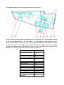
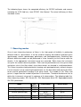
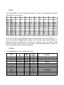
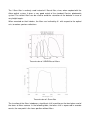
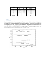
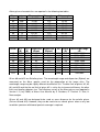
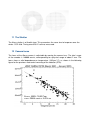
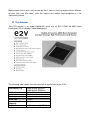
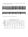
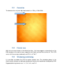
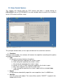
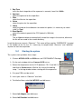
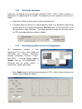
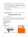
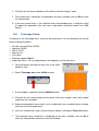
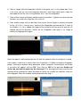
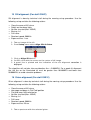
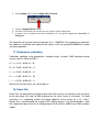
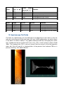
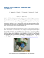
Afosc @1.82 m Copernico Telescope, Ekar User Manual L. Tomasella, S. Benetti, V. Chiomento, L. Traverso, M. Fiaschi Version 2.0 - March 2012 Note: In 2011 the old detectors (cooling system based on liquid nitrogen) mounted at the instruments of the Copernico 1.82m telescope was substitute with a new detector (based on Peltier cooler). The change of the CCD triggered an update of all the control system of both the telescope and the instruments. This technical report is a deep revision and an update of Version 1.2 (July 2003) of AFOSC User Manual by S. Desidera, D. Fantinel. E. Giro, H. Navasardyan. Some data, figures and tables which characterize Afosc were taken and readapted from this previous manual. The sections about the CCD and the control software are totaly new. The Asiago Faint Object Spectrograph and Camera (Afosc) is a focal reducer instrument. It allows wide field (8.7 × 8.7 arcmin field of view) imaging, low and medium resolution grism spectroscopy, polarimetry, and spectropolarimetry observations. Three wheels allow a selection of slits, filters, and grisms. The available grisms give resolutions up to 7300 (using the Volume Phase Holographic gratings and the 0.7 arcsec slit). The instrument was purchased from the Astronomical Observatory of Copenhagen. Similar instruments are DFOSC at Danish Telescope in La Silla, ALFOSC at NOT, BFOSC at Loiano. The full list of the FOSC instruments is available at: http://www.astro.ku.dk/~per/fosc/index.html AFOSC mounted on the 1.82 m telescope at M. Ekar Observatory. The following figure shows the optical layout of the instrument: Briefly, the light coming from the telescope passes through the slit (spectrographic mode) or the hole (imaging mode) in the slits wheel, it is redirected by a total reflection prism, and it is gathered by the collimator. In the collimated beam, between the collimator and the camera, the light passes through the filter wheel and the grism wheel where the reimaged exit pupil of the telescope is positioned. Finally the light is imaged by the camera on the detector. This table lists the basic optical parameters of Afosc: Collimator focal length Collimator linear field Beam diameter Camera focal length Camera linear field Reduction ratio Input fnumber Output fnumber Input scale Output scale Field of view CCD Pixel scale Wavelength coverage Limiting spectral resolution 234.27 mm 52.9 × 52.9 mm2 27.4 mm 159.35 mm 24.58 × 24.58 mm 0.68 f/8.97 f/6.10 12.64”/mm 18.59”/mm 8.85’ × 8.85’ 0.26”/pixel 3301100 nm 7350 The following figure shows the computed efficiency for DFOSC collimator and camera, excluding the CCD field lens, from DFOSC User Manual. The actual efficiency of Afosc should be similar. 1 Observing modes One of most interesting features of Afosc is the high grade of flexibility in performing different kinds of observations. It can be used for imaging, lowmedium resolution grism spectroscopy, echelle spectroscopy, polarimetry and spectropolarimetry. Switching from different observing modes can be performed in a few seconds (just the time to move the wheels), if the appropriate instrument setup was mounted. Table shows the instrument setup for the various observing modes. Filters can be positioned also in the grism wheel and grisms also in the filter wheel, since these wheels are located in a collimated beam. This allows to perform both polarimetric imaging and spectropolarimetry without changes in the instrument set up, mounting the polarimeter on the filter wheel and moving the filters to be used for polarimetric imaging in the grism wheel. The number of slits, filters and grisms is larger than the number of positions in the wheels. Therefore the observer has to define the instrument setup well in advance of its observations. The following table lists Afosc observing modes: ES: Echelle Slit PM: Polarimetric Mask SP: Spectropolarimetric Slit; POL: polarimeter. Mode Imaging Spectroscopy Echelle Spectroscopy Slit Wheel hole slit ES Polarimetry Spectropolarimetry PM SP Filter Wheel Grism Wheel filter hole grism (cross disperser) filter (or POL) POL hole grism grism POL (or filter) grism 2 Slits The following table lists the available Afosc long slits and the corresponding resolution achieved for the Afosc grisms: Slit Slit width width arcsec mm 0.68 0.054 0.84 0.067 1.26 0.100 1.69 0.134 2.10 0.167 3.02 0.240 4.22 0.335 8.44 0.670 16.87 1.340 Res. Gr #2 Res. Gr #3 Res. Gr #4 Res. Gr #6 Res. Gr #7 Res. Gr #8 Res. Gr #9 Res. Res. Gr #10 Gr #13 354 287 191 143 115 948 768 512 382 307 902 730 486 363 292 1403 1136 757 565 454 1707 1382 921 687 553 2769 2242 1494 1114 897 5316 4304 2869 2139 1721 303 245 163 122 98 5028 4070 2713 2023 1628 57 29 14 153 76 38 145 73 36 226 113 57 275 138 69 446 223 112 857 428 214 49 24 12 810 405 203 All the slits are 50 mm long, allowing to cover the whole field of view across dispersion. In grism echelle and spectropolarimetric modes such slit length causes spectral orders or polarimeter channels superposition. To avoid this, a proper short slit for echelle mode (width: 2.5 arcsec; length: 5 arcsec) and a short slit for spectropolarimetry (5 strips 2.5 arcsec wide and 22 arcsec long) were prepared. 3 Filters The following table lists the available Afosc filters: Filter U B V R I i OS1 ND1 ND2 ND3 ND4 ND5 λc nm 363.95 420.05 547.44 647.59 870.97 785 FWHM nm 34.54 72.82 89.90 156.98 236.26 180 Peak Transm. 0.53 0.71 0.94 0.86 0.97 0.90 0.1 0.01 0.001 0.0001 0.00001 Remarks Bessel Bessel Bessel Bessel Bessel Gunn Order Separator for Gr #13 neutral filter neutral filter neutral filter neutral filter neutral filter The i Gunn filter is routinely used instead of I Bessel filter, since, when coupled with the Afosc optical system, it gives a very good match of the standard Cousins photometric system. The neutral filters can be used to avoid the saturation of the detector in case of very bright targets. When mounted on their holders, the filters are inclined by 6° with respect to the optical axis, to reduce spurious reflections. Transmission of UBVRI Bessel filters. Transmission of i Gunn filter The insertion of the filters introduces a significant shift in position on the focal plane and of the focus of Afosc camera. In the following table, the focus shift is expressed in encoder counts, the zero point is the focus position without filters: Filter U B V R i NONE X shift px Y shift px 12.12 7.12 +10.84 +11.76 +2.5 +8.86 Focus Shift counts 8400 5000 2158 +921 +11500 0 4 Grisms Afosc is equipped with a large set of grisms. For a 1 arcsec slit the resolution of the grisms set range from ≈200 to ≈3600 and in each resolution domain. Blue, visual, and red grisms are available. Five VPH (Volume Phase Holographic, described in the following) grisms reach RS=5000, in the 5000Å9000Å wavelength ranges. The following figure shows the covered spectral range vs resolution for each available grism. Afosc grisms characteristics are reported in the following two tables: Grism #2 #3 #4 #6 #7 #8 #9 #10 #13 Grism #2 #3 #4 #6 #7 #8 #9 #10 #13 gr/mm 100 400 300 600 600 600 79 150 316 Blaze angle 7°15’ 15°00’ 14°36’ 22°00’ 34°00’ 54°00’ 63°30’ 5°24’ 63°30’ Prism glass OG515 LF5 LF5 LF5 LaK8 F8+OG515 LF5 UBK7 BaK2 λcen λblaze Dispersion Dispersion (Å) (Å) (Å/mm) (Å/pixel) 7200 7366 653 14.3 4300 3916 146 3.2 5800 5094 208 4.3 4000 3806 93 2.0 5250 5676 100 −2.2 7000 8161 84 −1.8 26 3900 3800 412 9.4 Prism angle 7°24’ 16°36’ 17°18’ 23°12’ 25°34’ 45°18’ 65°48’ 6°18’ 65°48’ RS 241 645 613 954 1161 1883 3615 206 3600 Purity Wavelenght range (Å) (Å) 3.1 5000 11000 6.1 3300 5700 8.3 3360 7740 4.0 3300 4900 4.9 4340 6580 4.3 6250 8050 See table 18.4 3300 7900 See table Grism #9 and #13 are Echelle grisms. The wavelength range and dispersion (Å/pixel) are measured on the Afosc spectra used for the preparation of the lamps atlas. The wavelength range may be slightly different for different slits. The blue limit of grisms #2, #3, #6, and #10 and the the red limit of grism #2 is set by the instrument efficiency; the other limits are fixed by detector size. The efficiency curves of the Afosc grisms are reported in Version 1.2 (July 2003) of Afosc User Manual by S. Desidera, D. Fantinel. E. Giro, H. Navasardyan. Grisms #2 and #10 are designed to be used as cross disperser for the echelle grisms (Grisms #9 and #13). However, they can be used also as normal grisms when a very low resolution spectrum with broad spectral coverage is required. 5 VPH: Volume Phase Holographic Grisms Afosc has been equipped with a set of VPH grisms. They allow to reach higher resolution than classical grisms, and with a rather high efficiency (typically about 80%). The basics of VPH technology are described in Giro et al. (2002). For the user, the VPH grisms behave very similar to normal grisms. Some line curvature is present and must be considered in the reduction. This table summarize the nominal characteristics of Afosc VPH grisms: Grism VPH #1 VPH #2 VPH #3 VPH #4 VPH #5 λcen (Å) 4680 5100 5890 6600 8700 W. Range (Å) 44304930 48495351 55216258 62386961 81959205 Dispersion (Å/mm) 20 20 30 29 41 Dispersion (Å/pixel) 0.27 0.27 0.40 0.39 0.55 RS gr/mm Angle 5000 5000 5000 5000 5000 2310 2310 1720 1720 1280 31.38° 34.60° 30.67° 34.60° 34.60° 6 Echelle spectroscopy Afosc offers the possibility to do intermediateresolution spectroscopy (RS ≈3600) covering a large spectral range using one of the two echelle grisms (#9 and #13) and using one of the lowresolution grisms as a crossdisperser (CD). Echelle mode is obtained mounting the echelle grism in the grism wheel and the crossdisperser in the filter wheel, turned 90 deg with respect to the normal grisms. The spectral format of Grisms #9 (+Grism #10 as cross disperser) includes 13 spectral orders, covering the whole wavelength range between 304 and 894 nm. The minimum separation between the spectral orders with this instrument setup is 8.3 arcsec (spectral orders 1920). Grism #13 has 4 spectral orders, not covering the full wavelength range as the individual orders are longer than the detector can accommodate. Grism #13 is intended mainly for use with an order sorter filter to give intermediateresolution spectroscopy with a long slit but it can also be used with one of the cross disperser grisms. In these cases, the minimum interorder separation is 62.8 arcsec (Gr #13 + Gr #2) and 61.5 arcsec (Gr #13 + Gr #10). This use is not recommended since spectra with similar spectral resolution and broader wavelength coverage can be obtained with Gr #9. 7 Wavelength Calibration The following lamps are available for the wavelength calibration: Argon (Ar), Helium (He), Neon (Ne), MercuryCadmium (HgCd), and Thorium (Th). Only three holders are available for the lamps. Th lamp is permanently mounted, since its holder is different from the other ones. In the other two it is possible to choose between Ar and Ne lamps and between He and HgCd lamps. The following table reports the main properties of the lamps. Lamp He Ar Th Ne HgCd Useful range (nm) 380730 7001000 3801000 570880 3601000 Nlines Remarks ≈10 ≈10 many ≈20 ≈20 line blending, Ar lines Ar lines The atlas for wavelength calibration, the suggested exposure times and the lamps to be coupled to each grisms are reported in the attached Afosc Atlas of comparison spectra. Due to lack of significant lines in some spectral regions, it could be useful to take spectra of two lamps and perform the wavelength calibration using the added spectrum: it is not possible to acquire simultaneously the spectra of two lamps. The spectra has to be taken separately and then added. 8 The pyramid focus A pyramid focus device is permanently mounted on the grism wheel. It allows determining the focus of the telescope or of the Afosc camera with a single exposure. The beam of light is splitted in 4 images. From the analysis of the relative positions of the four images, the best focus is evaluated. The use of pyramid focus from the Afosc control software is described in detail in the following (camera and telescope focus sections). 9 The Hartmann Masks The Hartmann Masks are two special masks selecting one half of pupil each one, used for the main calibration of the Afosc Camera focus. They can be installed on the grism wheel. 10 The ShackHartmann wavefront sensor A ShackHartmann wavefront sensor can be inserted in the grism wheel. It allows estimating misalignment between the primary and secondary mirrors and the amount of the residual optical aberrations. This device consists on an array of microlenses (size 1.0 x 1.0 mm), that samples a 27.8 mm diameter pupil, followed by a negative lens to obtain a suitable image of the spots on the detector. The picture shows the object image (a 5 th magnitude star) and the reference image obtained by illuminating the pinhole in the slit wheel with the dome flat lamp). The wavefront sensor and the results based on its use are described in detail in Pernechele et al. (2000). 11 The Shutter The Afosc shutter is of throttle type. This guarantees the same level of exposure over the whole CCD field. Timing error of 0.12 sec was measured. 12 Camera focus The focus of the Afosc camera is adjustable by moving the camera lens. The total range of the encoder is 140000 counts, corresponding to a physical range of about 2 mm. The focus shows a mild dependence on temperature (10.3µm/°C), as shown in the following figure for the previous mechanical mounting of the detector (SITe). Measurement of the focus shift caused by filters shows a clear zero point offset, different for each filter (see filter table), while the slope of the relation focus/temperature is not significantly altered. 13 The detector The CCD camera is an Andor DW436BV which use an E2V CCD4240 AIMO back illuminated CCD as detector (2048X2048 pixels). The following table reports the main physical characteristics of the CCD: Horizontal CTE Active Area prescan postscan pixel size pixel full well capacity Dark current 0.999 999 86 @62kHz 0.999 999 46 @500kHz 2048×2048 pixels 50 pixels 42 pixels 13.5µm 100ke (nominal) 0.001 e/px/sec @ 75°C Gain, readout noise, readout time and bias level is related to the selected read out speed of 31 kHz, 62 kHz, 500 kHz and 1 Mhz: Read out speed → gain (e /ADU) readout noise (e) full frame readout time (sec) overscan bias level (ADU) Read out speed → Bin 1x1 full well Bin 2x2 full well 31kHz digital sat. digital sat. 31kHz 0.95 3.0 142 5 62kHz ~55k ADU digital sat. 62kHz 1.93 3.0 71 20 500kHz ~39k ADU >64.2k ADU This figure shows the CCD nominal quantum efficiency: 500kHz 2.73 7.6 9 360 1MHz 2.9 10.4 5 1690 1MHz ~36.5k ADU >62.5k ADU 13.1 Cosmetics The detector has only one big trap located at x=708, y=12682048. 13.2 Field of view With the instrument rotator in the default position, the image appears automatically on the DS9 window at the end of every exposure with North up and East to the left. The CCD scale is 0.26 arcsec/px (unbinned) and FOV is 8.7’X8.7’ 13.3 Windowing and binning It is possible to window the CCD to reduce readout time. The windowing boxes in the Afosc control software are defined according to the physical coordinates displayed by DS9. Supported binning formats are: 1×1, 2×2, 4×4, and 2×1. 14 Afosc Control System The software that controls both the CCD camera and Afosc is started clicking on CCD+AFOSC icon on PCSTRUMENTI; the main window allows to recall all the functions for the CCD control and Afosc setup. This principal window shows, on the right, ten identical lines and eleven columns: 1. Checkbox Ticking on the checkbox, the software will execute the exposition according to the options selected in that ticked line. 2. Type it is possible to choose between five options: a. Object: during the exposition the shutter is open. b. Dark: during the exposition the shutter is close. c. Flat: during the exposition the shutter is open. d. Skyflat: as “illum” in IRAF, during the exposition the shutter is open. e. Bias: time integration null, with the shutter close. f. Calib: during the exposition the shutter is open with the selected Lamp switch on. 3. Repeat It is possible to automatically repeat the same exposition, from 1 to 9999 times. 4. Identifier insert the name of the object. This name will be used for “OBJECT” keyword in the header of the fits file. 5. Exp Time insert the time integration of the exposure in seconds, from 0 to 10000s. 6. Aperture select the aperture for the exposition. 7. Filter select the filter for the exposition. 8. Grism select the grism for the exposition. 9. Lamp select the lamp for the calibration: to enable this option, it is necessary to select “calib” in Type. 10. Read Speed select the read out speed of the CCD (default is 500 kHz) 11. Save Tick on Save checkbox to automatically record the image in the archive, otherwise the file will be saved in the scratch directory. Insert the observer name in “Observer”. This name will be used for “OBSERVER” keyword in the header of the fits file. It is necessary to compile both “Observer” and “Identifier” squares to start the acquisition. 14.1 Starting the system The system startup follows these steps: 1. Click on AFOSC+CCD and DS9 icons on PCSTRUMENTI Desktop. 2. On the main window click on Connect CCD botton. 3. Select the temperature for the CCD (between 70°C and 80°C) and click on Cooler botton. Wait for the “end of the cooling ramp...” in the log window, before starting with the exposures. 4. Only one DS9 must be active! 5. Insert your name in “Observer” text field. 6. To initialize Afosc select Init AFOSC from Init menu. 7. Select Init Adapter from Init menu. 8. Select Init Rotation from Init menu. 14.2 Defining exposures Exposures are defined using the principal window of CCD + Afosc Control software, as explained at the beginning of this section. The properties of each exposure can be set as follows: 1. filling the text fields of one or more of each equivalent line. 2. If needed, rotate the flange at a selected position angle (e.g. parallactic angle) filling the text field with the angle and clicking on Set Rot button. On the right there is the PA (parallactic angle) calculator. The flange parallactic angle can also be read in the TPS (telescope pointing software) window. 14.3 Selecting a guide star for the Autoguiding The Autoguiding software is fully explained in The 1.82 m Ekar Copernico Telescope User Manual (Tomasella, Benetti, Chiomento, Traverso, Fiaschi, Feb. 2012). One the Guider software (Guider icon on PCCOORDINATE) is initialized and the guide camera is switched on, follow these steps: 3. Press Probe button from the principal window of CCD + Afosc Control software; the Guider Probe window will appear: 4. Press Reload Map button to refresh the display of GSC stars in the Afosc field. 5. Find a good star for autoguiding both in the strip on the right or on the left of Afosc field, click on it with left mouse button than on Go Coords button and the probe will move to the selected position. You can also move the probe using the four arrows which are on the topleft of the Guider Probe window. 6. Start the autoguiding from the Guider software (see The 1.82 m Ekar Copernico Telescope User Manual). 14.4 Executing exposures 7. Click on Start Sequence button. You can repeat ntimes the same sequence filling the text field with a number (n). 14.5 Camera Focus The Afosc camera focus is determined by the technical staff during the setup operations. If the Afosc temperature changes more than 2°C during the night, it might be useful to make the camera focus procedure using the following telescope and Afosc procedure: • • • • • • • • • Open the cover of M1 mirror Switch on the dome lights No filter inserted (Filter: NONE) Aperture: pinhole (MF) Grism: PYFO Binning 1x1 Full frame Read out speed: 500KHz Exposure time: 10 sec 1. Take and image; the beam is splitted in four: 2. Select Camera focus from Utilities menu. 3. A new window is opened: click on select spot button. 4. Click with the left mouse button on the center of the four image's spots. 5. The camera focus correction is displayed on the focus window: click on Go to reach the new position. 6. If the new camera focus is very different from the precedent one, it might be useful to repeat the procedure (the new focus adjustment should be lower than 1000 counts). 14.6 Telescope Focus To determine the telescope focus using the pyramid focus use the following setup and take the following actions: • • • • • • • No filter inserted (Filter: NONE) Aperture: NONE Grism: PYFO Binning 2x2 Full frame Read out speed: 500KHz Exposition time: > 10 sec (depending on the brightness of the field stars) 1. Take and image; the beam of each star in the field is splitted in four: 2. Select Telescope focus from Utilities menu. 3. A new window is opened: click on Add Star button. 4. Click with the left mouse button on the center of the four image's spots (with a good segnal but not saturated). 5. Repeat the procedure from step 3 so as to add other stars for obtaining an avarage measure of the telescope focus. 6. If the last selected star shows a bad measure, delete it clicking on Clear last button. 7. The telescope focus correction is displayed on the focus window: click on Go to reach the new position, otherwise close the window. 8. If the new telescope focus is very different from the previous one, it might be useful to repeat the procedure (the new focus adjustment should be lower than 0.05 mm). It is advisable to do the telescope focus when the telescope position changes significantly and if there is a sensible temperature variation during the night. To be done after the procedure of camera focus. 14.7 Combine offset The Combine Offset procedure allows to calculate the distance between the actual position of the target and the desired position and to put in a simple and fast way the object in the slit. The steps are the following: 1. Take an image without filter and slit to recognize the target position in the field. 2. Select Combine offset from Utilities menu. 3. A new window will appear: select the slit and click on Grab coords (if the target is faint) or Grab centroid (if the target is bright) buttons. 4. Click on your target in DS9 image with the left mouse button and then Go on the opened window. 5. The telescope tracking and the autoguider will be automatically switch off; both the telescope and the probe will move to the new position; at the end of the procedure, the telescope tracking will be resumed. 6. Take an image with the Autoguider to check if the guide star is in the guider box: if this is the case, you can start the Autoguide; otherwise, with Video mode active, move the telescope to have the star in the guide box, then start the Autoguider. 7. Take another image and repeat combine offset calculations. Typically no more than two iterations are necessary to put the star in the slit. 8. Take another image with the desired slit to control that the target is perfectly centered on the slit. If this is not the case, switch off the Autoguider and change the Y value of the Guider: if +1 unit is added, the target will be shifted of 0.45 arcsec to N (with the slit aligned along EW direction). Switch on the Autoguider and repeat a slit image to control the target position again. When the object is well centered on the slit, take the spectrum with slit and grism inserted. If the target is more than 2 arcmin from the slit position, it is better to stop the Autoguider before starting the combine offset procedure (steps 2 onward). A warning that the Guider is not active will appear, click on OK. Then click on YES to the question Guider not Active: do you want to move only the telescope? The telescope will move and then the tracking will be switched on. Move the probe to search for a guide star and then switch on the Autoguider. Start the combine offset procedure from step 1. 15 Slit alignment (For staff ONLY!) Slit alignment is done by technical staff during the morning setup procedure. Use the following setup and take the following actions: • • • • • • • Close the cover of M1 mirror Switch on the dome lights No filter inserted (filter: NONE) Binning 1x1 Full frame Read out speed: 500KHz Exposure time: 1 sec 1. Take an image of the slit. 2. From Setup menu select Align Slit & Grism. 3. Click on Align Slit button 4. On DS9, click with the mouse on the center of slit image. 5. A green line is plotted and the indication of the slit alignment correction is displayed. The algorithm will not take into consideration flux < 5.000ADU. For a good slit alignment the, the flux on the illuminated slit must be greater than 10.000ADU and lower than 50.000ADU, to avoid saturation problems. 16 Grism alignment (For staff ONLY!) Grism alignment is done by technical staff during the morning setup procedure. Use the following setup and take the following actions: • • • • • • • • Close the cover of M1 mirror telescope and dome in Flat Field position Flat field lamp 1kW switched on No filter inserted (filter: NONE) Binning 1x1 Full frame Read out speed: 500KHz Exposure time: 20 sec 1. Take a spectrum with the selected grism. 2. From Setup menu select Align Slit & Grism. 3. Click on Align Grism button 6. On DS9, click with the mouse on the center of the spectrum. 7. A green line is plotted and the indication of the grism alignment correction is displayed. The algorithm will not take into consideration flux < 1.000ADU. For a good qrism alignment the spectrum should be well exposed, but counts must not exceed 50.000ADU to avoid saturation problems. 17 Photometric calibration Calibration equation using photometric standard fields (Landolt, 1992) obtained during several nights in 2010 and 2011: U – u = 21.13 + 0.106 (U – B) B – b = 24.06 + 0.037 (B – V) V – v = 24.85 + 0.062 (B – V) R – r = 24.65 + 0.043 (V – R) I – i = 23.79 + 0.030 (R – I ) Where the constant terms are calculated in e. 18 Dome Flat Dome flats are obtained at the beginning of each Afosc run by the technical staff using one of the two lamps (0.3 and 1.0 kW) projected on the white screen in the dome. To avoid saturation, it is suggested to point the lamps opposite to the screen for V, R, i filters. Master flat is recommended for a good CCD fringing removal. The following tables show the suggested exposure times for imaging dome flat for 62kHz, 500kHz and 1MHz readout modes: Filter U B V R i Filter U B V R i 1kW Lamp Flux (e px1 s1) 700 6150 3000 6500 7250 Lamp 1kW 0.3kW 1kW 1kW 1kW 0.3kW Lamp Remarks flux (e px1 s1) 200 2050 1000 2150 2400 bin 1x1 120s 35s 25s 12s 11s Dome screen Dome screen Lamp opposite to the screen Lamp opposite to the screen Lamp opposite to the screen bin 2x2 30s 10s 6s 3s 2.5s Remarks Dome screen Dome screen Lamp opposite to the screen Lamp opposite to the screen Lamp opposite to the screen 19 Spectroscopy Flat Fields Flat fields for spectroscopy are also obtained at the beginning of each Afosc run by the technical staff using one of the two lamps (0.3 and 1.0 kW) projected on the white screen in the dome. The Afosc stability is very good, allowing to take flats during daytime. Some tests showed that flexures amount to 0.1 px or less, with a small hysteresis effect (Claudi 1998). The fringing of the CCD is not very strong. From the analysis of flat field spectrum taken with Grism #2 and #4, a fringing pattern at few percent level redward 750 nm is present, reaching ~10% above 900 nm.