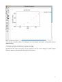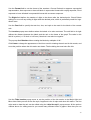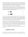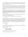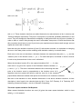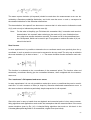
1
pro Fit 6.2 User Manual
http://www.quansoft.com/
© 1990-2010 by QuantumSoft
All rights in this product are reserved.
End User License Agreement
License terms:
1. The Software and its related documentation are provided "AS IS" and without warranty of any kind. QuantumSoft disclaims all other warranties, expressed or implied, including, but not limited to, the implied warranties of merchantability and fitness for a particular purpose. Under no circumstances shall QuantumSoft be
liable for any incidental, special, or consequential damages that result from the use or inability to use the
Software or related documentation, even if QuantumSoft has been advised of the possibility of such damages. In no event shall QuantumSoft's liability exceed the license fee paid, if any.
2. Rights granted:
a) Use of the "trial" version of the Software is granted within the limits built-into the trial version application.
b) Use of the "full" version of the Software is granted for n users, where n is the number of users indicated in
the purchase acknowledgement for the registration key bought from QuantumSoft or from one of its resellers. An n-user license is deemed to be exceeded if the Software is installed on more than n computers.
Exception: Right is granted within the single user license to install the Software on two computers simultaneously if both said computers are regularly used by one person only.
Within this agreement, "installed" on a computer means that the Software can be executed on said computer, either because it is stored locally on said computer or accessible by said computer through a network.
3. Competent court and law:
This Agreement shall be governed by the laws of Switzerland and the competent court is in Zürich, Switzerland.
4. If, for any reason, any provision of this Agreement, or portion thereof, is found to be unenforceable under
the applicable law, that provision of the Agreement shall be enforced to the maximum extent permissible so
as to effect the intent of the parties, and the remainder of this Agreement shall continue in full force and effect.
5. QuantumSoft reserves the right to change this agreement at any time. Any changes will be announced at
www.quansoft.com.
6. Pre-release software: By using any alpha or beta version (pre-release version) of the Software, you acknowledge that you are aware that such versions are for testing purposes only and that they often contain
substantial errors that affect their functionality or may damage data on or functionality of a computer. Prerelease versions of the Software should never be used on computers containing data critical for your work.
QuantumSoft
Bühlstr. 18
CH-8707 Uetikon am See
Switzerland
2
Copyright!
pro Fit © QuantumSoft 1990-2010
!
All rights reserved. No part of this publication or the program pro Fit may be reproduced, transmitted, transcribed, stored in a retrieval system, or translated into any
language or computer language in any form or by any means, electronic, mechanical,
magnetic, optical, chemical, manual, biological, or otherwise, without prior written
permission of the publisher.
!
The information in this user's guide is subject to change without notice.
Trademarks!
Macintosh and LaserWriter, Finder, Mac OS, Mac OS X, PowerBook, Quickdraw,
Quartz, Power Macintosh, Macintosh Programmers Workshop (MPW), and Xcode are
registered or non-registered trademarks of Apple Computer, Inc. PostScript is a registered trademark of Adobe Systems Incorporated.
!
"Python" and the Python logos are trademarks or registered trademarks of the Python
Software Foundation (www.python.org). They are used with permission of the Foundation.
!
pro Fit is a trademark of QuantumSoft, Zürich
Customer Support!
The main resource for customer support is the QuantumSoft webpage at
www.quansoft.com. Additional customer support is provided on a discretionary basis
by e-mail at the address [email protected].
3
Table of contents
1. Introduction!
This handbook!
Key features!
System Requirements!
A note on updates!
9
9
9
10
11
2. Basic concepts!
12
3. Getting started!
A first session!
Our data!
Entering the data!
Plotting the data!
A function to fit our data!
Fitting!
Defining your own functions!
pro Fit Pascal and Python!
Writing programs!
13
13
13
13
15
17
19
22
24
25
4. Working with data!
Data editing!
The data window!
Data types!
Permanent transformations!
Entering data!
Transforming data!
Defining a data set to work on!
27
27
27
28
30
30
31
32
5. Working with functions!
Editing in the parameter window !
Using functions!
Viewing function outputs!
Calculating output values!
Optimization of functions!
Analyzing functions!
The Spline function!
33
35
36
36
36
36
36
37
6. The Preview Window!
The basics!
Preview Window Appearance!
Preview Window Tools!
Managing coordinate markers!
Tips and tricks!
Using the preview window during a fit!
Choosing initial values of function parameters!
39
39
42
42
44
45
45
45
7. Drawing and Plotting!
The drawing window!
Drawing tools!
Coordinates, accuracy and drawing info!
Drawing objects!
Shape properties!
47
47
47
48
49
49
4
Drawing windows in dialog mode!
Editing drawings!
General drawing commands!
Objects created with the tools palette!
Editing polygons and lines!
Data Points!
Control shapes!
Editing drawing objects!
Exporting pictures!
File formats for graphics exports!
Import graphics!
Plotting!
Plot types!
Axis types!
Plotting a function!
Plotting a two-dimensional data set!
Plotting a three-dimensional data set!
Graphs and legends!
Editing legends!
Editing graphs!
Panel “Frame”!
Panel “Grid”!
Panel “Bar charts”!
Graph Styles!
Graph coordinates and zooming!
8. Fitting!
Mathematical background!
The mean square deviation: Chi-Squared!
Zero X-errors!
The “usual case”: Chi-squared and zero x-errors!
Error analysis and confidence intervals!
Fitting algorithms!
The Monte Carlo algorithm!
The Levenberg-Marquardt algorithm!
The Robust minimization algorithm!
The Linear Regression algorithms!
The Polynomial fitting algorithm!
Goodness of fit!
Literature and suggested reading!
The fitting process!
General features!
Parameter limits!
Running a fit!
Inspecting the progress of a fit!
Error analysis and confidence intervals!
Fitting results!
Using the various fitting algorithms!
Using the Levenberg-Marquardt algorithm!
Using the Robust minimization algorithm!
Using the Monte Carlo algorithm!
Using the Linear Regression algorithm!
Using the Polynomial fitting algorithm!
Fitting multiple functions and x-values!
General hints for fitting!
50
51
51
53
55
56
58
59
60
60
61
62
62
64
65
69
72
72
73
74
83
84
85
87
89
90
90
93
94
94
95
95
96
96
99
100
101
101
102
102
102
103
103
106
106
107
107
108
108
108
109
109
109
111
5
Starting parameters!
Redundancy of parameters!
111
111
9. Defining functions and programs!
113
Introduction!
113
Built-in languages for creating new functions and programs!
114
Introduction to Python and Pascal programming in pro Fit!
115
A simple program!
117
A simple function!
118
Using the Python language!
120
Introduction!
120
Python: Defining programs!
120
Python: Defining functions!
122
The module pf!
124
Compatibility notes!
124
Using the pro Fit Pascal language!
125
Introduction!
125
Pascal: Defining functions!
125
Pascal: Defining programs!
129
pro Fit Pascal in depth!
129
On-line help for programming!
129
The help menus!
130
Browsing functions and programs!
130
Finding the definition of a symbol!
131
The compiler!
131
Advanced function and program definitions!
131
Initializing and shutting down programs and functions (Initialize, xxx_init)! 131
Input value checking (Check, xxx_check)!
133
Input value pre-calculations (First, xxx_first)!
135
Calculating derivatives (Derivatives, xxx_derivatives)!
136
Finishing up (Last, xxx_last):!
137
Determining how multiple output values are rendered in the preview window !138
Programming examples!
140
Accessing data!
140
Drawing!
142
pro Fit Objects!
143
Automatic Macro Recording!
144
External functions and programs!
144
Debugging window!
145
Using pro Fit plug-ins!
147
Saving functions and programs as plug-ins!
147
Loading Plug-ins!
147
Removing functions and programs from the menus!
147
Loading plug-ins automatically on startup!
147
Loading a set of plug-ins together with a new preferences file!
148
Attaching scripts!
148
Working with controls in drawing windows!
151
Working with plug-ins!
Creating a plug-in with a compiler!
Writing an a plug-in with an external compiler!
Routines to be modified!
Routines to be defined in functions and programs!
Routines to be modified in external programs only (not used for functions)!
Routines to be modified in external functions only (not used in programs)!
156
156
158
158
158
159
159
6
Predefined constants and types!
Global variables!
Procedures provided by pro Fit!
162
163
163
10. Apple Script!
Batch processing!
When to use Apple Script!
pro Fitʼs Apple Script dictionary !
164
165
168
168
11. Printing!
Printing from pro Fit!
Printing a pro Fit drawing from another application!
169
169
169
12. Preferences!
171
13. General features!
Help !
Help tags!
On-line evaluation of mathematical expressions!
File info!
Shortcuts and other options!
172
172
172
172
174
175
Appendix A: About numbers!
Floating point numbers!
Date and Time data!
178
178
178
Appendix B: File formats!
Data!
The default text format!
Importing text files!
Saving text files!
The native data format!
Drawings!
Image formats!
179
179
179
179
180
181
181
182
Appendix C: Python compatibility notes!
183
Appendix D: pro Fit Pascal Syntax!
Introduction!
Program definition syntax!
Function definition syntax!
Types!
Simple numeric types:!
Complex type:!
Matrix and Vector types:!
String and char types:!
Arrays!
Loop statements!
The for loop !
The while loop!
The repeat loop!
Optional parameter lists!
Aborting procedures, functions and programs!
Predefined constants, functions, procedures, and operators!
Functions and procedures provided by pro Fit!
185
185
185
187
190
191
191
192
194
195
195
195
196
196
197
198
199
200
7
Comparison to standard Pascal!
200
8
1. Introduction
This handbook
This handbook is a conceptual introduction that describes key features and concepts and provides
some step by step recipes. It is neither a reference to all of pro Fitʼs commands nor to its scripting
environment – such reference material is included in pro Fitʼs online help.
Key features
pro Fit is an interactive tool for the investigation, analysis and representation of functions and data.
It is designed for users in science, research, engineering, and education. The key features of
pro Fit are:!
• Spreadsheet and data management: Numerical and alphanumerical data can be stored, transformed and analyzed. Predefined and user defined algorithms can be used for data transformation.
• Analysis of mathematical functions: The values passed to mathematical functions and those returned from them are managed in a parameter window that allows to easily determine which
input values must be used to calculate the output values of the function. Input values can be
easily edited and managed and the effects of any change in their values are previewed interactively and in real time.
• Customized functions and algorithms: pro Fit provides very powerful and simple methods for
defining mathematical functions, programs, data transformation algorithms, drawings, and general macros.
• Simple, built-in Pascal-like compiler for user-defined functions and programs. This is a version
of Pascal adapted to the needs of the pro Fit environment and extended to support floating point
numbers, complex numbers, vectors, strings, and up to 4x4 matrices as general data types to
be used in any mathematical expressions.
• Built-in support for Python for user-defined functions and programs. See www.python.org for
more information.
• Support for Apple Script. Apple Script is the high-level scripting language of Mac OS, used to
automatize tasks and control applications.
• Interactive parameter modeling and curve fitting: A key feature of pro Fit is its intuitive and flexible interface for modeling and fitting data, offering the choice of several fitting algorithms and
optional restriction of parameter ranges. Fitting supports y- as well as x-errors and allows a
Monte-Carlo error analysis for fitted parameters. A parameter can also be fitted manually by
dragging the functionʼs curve with the mouse.
9
• Professional plotting: Data and functions can be plotted in a multitude of ways in high-quality,
publication-ready graphs. Plots can have multiple coordinate axes using linear, logarithmic, 1/x,
and normal probability scalings, including reverse scaling. Plotting types include scatter plots,
line plots, skyline plots, histograms, contour plots, color plots, and box plots. Interactive 3D
models of function and data can be generated and edited through the 3DplotterGL plug-in.
• Built-in drawing editor: A complete range of drawing tools allows flexible editing and annotation
of plots and presentations. Specific drawing objects such as buttons, check boxes, and pop-up
menus are supported to be used as interfaces for user-defined programs.
• Extensive graphical output possibilities: Pro Fit supports output and, in part, input for the following graphic formats: PDF, PostScript™, EPS, PICT, high resolution bitmaps, PNG, TIFF, GIF,
JPEG.
• Scriptability and Recordability. You can record your actions automatically as a pro Fit program
or Apple Script, Pascal or Python script for replaying them later.
• Externally compiled code: It is possible to define functions, algorithms, and other programs using an external programming environment and compiler and to import them as plug-ins. pro Fit
can also be controlled via Apple Script.
• On-line evaluation of mathematical expressions: Enter any mathematical expression wherever
pro Fit expects numerical input (such as in spreadsheets or dialog boxes).
• Drawing from a script: pro Fit scripts can directly draw into pro Fitʼs drawing windows to create
drawings with high precision coordinates. These drawings are available for copying and pasting
into other applications and for high-resolution printing.
• Scripting: Write complete macros to perform common tasks such as opening and closing document windows, fitting, importing and exporting files, etc. using either Apple Script, Python or a
Pascal-like scripting language
• Debugging environment: A powerful debugger provides tools for developing and debugging
complex scripts.
• Extensive on-line help: An on-line help system provides answers, hints and explanations.
• Plug-ins: Various plug-ins further increase pro Fitʼs power, e.g. for contour plotting and 3D plotting of functions and data sets.
• And much more...: Such customizable data file import and export, services, multi-dimensional
functions, etc.
System Requirements
pro Fit 6.2 has been developed for Mac OS® 10.6 or better. Compatibility with earlier systems has
not been tested, even though pro Fit 6.2 will probably also work (mostly) on MacOS 10.5.
10
For users interested in running a version of pro Fit on older systems and machines, pro Fit 5.1
through 6.1 are still available upon request:
pro Fit 5.1 is MC 680x0 based.!
pro Fit 5.5 is Power PC based and allows to save most of its documents in pro Fit 5.1 format.
pro Fit 5.6 requires Mac OS X 10.0.4 or later, or Mac OS 9 with CarbonLib 1.3 or later.
pro Fit 6.0 requires Mac OS X 10.3 or later.
pro Fit 6.1 requires MacOS X 10.4 or later.
pro Fit 6.2 requires MacOS X 10.6 or later.
A note on updates
Development of pro Fit continues. To check for updates to your current version, visit QuantumSoftʼs web site at http://www.quansoft.com/.
You can also use pro Fitʼs built-in mechanism for checking for updates. Choose “About pro Fit”
from the application menu and click the button “Check for newer versions”. pro Fit will contact our
servers and tell you about any updates that you may want to download.
11
2. Basic concepts
pro Fit works with data, drawings, functions and scripts.
You can enter data into spreadsheet windows. Data can be analyzed, plotted, and transformed.
For transforming data, you can use built-in transformation algorithms, (e.g. sort, transpose, filter,
Fourier transform, or mathematical operations) or user-defined ones. Data can be text, numbers
and dates.
You can define your own data transforms by writing scripts (programs), which can e.g. access the
data in the spreadsheet windows. pro Fit supports the following scripting languages:
- Apple Script (e.g. in conjunction with AppleScript Editor)
- Pascal (more accurately a Pascal-like scripting language) executed within pro Fit
- Python scripts executed within pro Fit
Functions can be used for plotting, analysis, and curve-fitting. There are a number of built-in functions (such as log, cos, exp, etc.). You can define your own functions using Pascal or Python.
Functions and scripts can also be created using an external compiler (plug-ins).
Functions can be analyzed and they can be fitted to data. pro Fit provides powerful fitting tools
based on various algorithms and methods. Fits can be multidimensional, parameters can be constrained, and their starting values can be selected manually or, depending on the function and algorithm to be used, automatically.
You can plot your functions and data sets in a drawing window. pro Fit offers most standard features of a drawing program, and the appearance of all graphical elements is customizable.
These various elements of pro Fit are described in the following sections.
12
3. Getting started
A first session
This chapter describes a typical pro Fit session. It shows how to enter new data, plot it, and how to
fit a mathematical function to it.
Our data
The worldʼs human population is growing rapidly. The following table shows the number of inhabitants of this planet for the period after 1940.
year
population (in millions)
1940
2200
1950
2500
1960
3000
1969
3600
1975
4000
1981
4400
1987
5000
1990
5300
Let us plot and analyze these figures.
Entering the data
First, you must import your data into pro Fit. To do this, open a new data window:
1. Choose “New Data...” from the File menu:
An empty data window appears:
13
Data are arranged in horizontal rows and vertical columns. The topmost cell of each column shows
the name of the column (by default ʻColumn 1ʼ, ʻColumn 2ʼ, etc.). The cells below contain the data
of each column.
2. Click into the first empty cell of column 1 and enter the first year, 1940.
We fill the first column with the years and the second column with the population.
3. Click into the first cell of column 2 and start entering the population data,
Enter the values given in the table above. Note that you can use the arrow keys, the tab and the
return or enter key to move from one cell to another.
4. Enter the column titles, ʻyearʼ and ʻpopulation in millionsʼ.
Click into the titles ʻColumn 1ʼ or ʻColumn 2ʼ and enter the new names. Move the mouse to the vertical separation line to the right of the second column title, click, and drag the separation line a little
bit to the right, so that you see the complete title. (Itʼs also possible to customize the appearance
and formatting of numbers and text).
5. Save the data by choosing “Save As...” from the File menu.
You are prompted to enter a name for your file. Your window should now look like this:
14
Plotting the data
Now that we have entered the data, we can display it graphically.
1. Choose “Data y(x)...” from the Plot menu
A dialog box appears where you can enter the ranges of the plot, the columns to be plotted, and
more. In this introductory session we can use the settings as they are.
2. Click OK.
A drawing window appears, showing a graph of the data.
15
You can edit a drawing easily. For example, you can change most parts of the graph just by
double-clicking.
3. Double-click the vertical axis to change its range.
(Double-click the vertical axis itself, not the numbers to the left of it!) A dialog box called “Graph
Settings” appears, presenting the settings of the left y-axis:
16
You can change a variety of things here. Often you will use the edit fields First and Last to set the
range of the axis. Another important field is the ʻDistanceʼ field that defines the distance between
major tick marks.
4. Enter 0 for First and 6000 for Last, then click OK.
The vertical axis of the graph now starts at 0 and ends at 6000.
Double-click other parts of the graph or its legend to change other attributes. Try double-clicking
the horizontal axis, the center of the plot, or the dot representing the data points in the legend. You
can also double-click any text in the drawing to change it. Or you can choose any of the drawing
tools to add lines, polygons, text, etc.
A function to fit our data
The growth of a population can often be described by an exponential function of the type
17
!
,!
(3.1)
where p(t ) is the population at time t, p(x0) the population at an arbitrary start time x0, and t0 its
growth constant.
Let us try to investigate the validity of this formula for the worldʼs population. We want to find the
set of parameters for which equation (3.1) fits our data best.
1. Choose Exp from the Func menu
This selects the built-in exponential function as the current function to be used for analysis, fitting,
and plotting. It also brings the parameters window of the Exponential function to the front. This
window gives a description of the exponential function and its parameters:
The window is divided into three regions. The top region provides a short description of the selected function. The central part displays the input and output values of the function, and lets you
edit input values. The bottom region displays additional information on the selected input or output
value.
The function Exp looks like this:
!
,!
(3.2)
which is essentially identical to equation (3.1). The parameter window also displays the default
values for the parameters (input values) A, t0 and const. Starting from these parameters, pro Fit
can find a better set of parameters for describing our data. But first you must define which parameters you want to fit, i. e. which parameters you want to vary in order to approximate the data with
the Exponential function.
As mentioned above, the starting time x0 is arbitrary. Let us set it to 1940.
2. Click the number beside ʻx0ʼ in the parameters window and enter 1940.
This defines the parameterʼs value and the starting value that will be used for curve-fitting.
18
Since x0 is arbitrary, we do not want to fit it:
3. Uncheck “Use for fitting”.
(The check box “Use for fitting” can be found in the lower right corner of the parameter window
when a parameter is selected. As a shortcut, you can also simply click a parameter name to toggle
its status.)
The parameter name changes from bold face to plain text. This indicates that this parameter is
constant and will not be fitted.
4. Click the parameter name ʻconstʼ
We donʼt want to fit this parameter, either. The parameter name is not bold anymore and the option
“Use for fitting” is unchecked now.
Fitting
1. Choose Curve Fit... from the Calc menu
This is the command you use to set up the various options used for fitting, such as the correspondence between data columns and default input and output values of a function, data errors, etc.:
The data column settings are already ok.
19
2. Click the button “Fit” to start fitting
Fitting is very fast. When it is completed, the fitted function is shown in the plot preview in the lower
half of the fitting window.
The fitted parameters appear in the results window:
The fit yields –54 years for t0 and 2113 millions for A. Note that above we wanted to show you the
fitting dialog box. For simple fits, you can also execute them directly by using the Simple Curve Fit
command in the Calc menu, which simply reads its information from the current data window and
immediately executes a fit without asking for any additional details.
20
We can plot function (3.2) using the fitted parameters:
3. Choose Plot Function f(x)... from the Plot menu
A dialog box appears, displaying options for plotting the function:
We donʼt need to change any of these options.
4. Click OK to draw the curve
The curve is drawn in the graph. You can now rearrange the items in the drawing window to obtain
a representation of data and theory like the following:
21
population in millions
population.data
population in millions
theory
5000
4000
3000
2000
1940
1960
year
1980
Defining your own functions
In the previous session you have fitted the built-in exponential function to your data. Fine. But what
do you do if your model is described by some mathematical equation that does not appear among
the built-in functions in the Func menu?
Define your own function! pro Fit can work with virtually all functions you can think of. Let us look
at an example. Imagine you want to analyze a function of the form
y = a sin(x) × ln(x) + b
(3.3)
with the parameters a and b. To define this function:
Choose New Function from the File menu.
This opens a new, empty function window.
Enter the definition of your function in the new window.
Just enter:
!
a[1]*sin(x)*ln(x) + a[2]
on the first line.
Click the "To Menu" button in the function window, or choose “Compile & Add To Menu”
from the Customize menu.
This translates your function into computer code.
pro Fit looks at what you wrote and sees that you used the standard input (x) and the standard parameter array (input values) a[1], a[2]. It therefore assumes that you want to define a new function
and interprets your text accordingly.
22
The new function is added to the Func menu, and the parameter window shows its default parameters.
Your simple expression is replaced by a complete, syntactically correct function definition:
!
!
!
!
function User_Function;
begin
! y := a[1]*sin(x)*ln(x) + a[2];
end;
The first line defines the name of the function as it appears in the Func menu (User_Function is
the default proposed by pro Fit. You can change it to something like LogSine). Then, enclosed
between begin and end, there follows the definition of the function. In the third line the function is
calculated (from the variable x and the parameters a[1] and a[2]), and it is assigned (“:=”) to
the variable y.
Note:
An alternative way to define the same function is:
function logSine(ampl, offset:real);
begin
!
y := ampl*sin(x)*ln(x) + offset;
end;
In this definition, the parameters (input values) of the function are defined in the function header.
The names used in the header are then used in the function body. This is the syntax used for standard Pascal functions. pro Fit uses the parameter names defined in the function header for displaying the parameters in the parameters window.
After adding the function to pro Fit, you can change its parameters in the parameters window. You
can plot the function, use it for fitting, calculations, etc.
To plot it, you should first set its parameters to reasonable values, e.g. 1 and 0.5: Enter these values in the Parameter window and choose “Plot Function...” from the Draw menu. In the dialog box
that comes up, select the plotting range (e.g. the x-axis from 0 to 5). If you already have an open
drawing window, you should check the option “Open New Window”, otherwise your curve will be
drawn into the existing graph.
Our sample function is not defined for x<=0. If you were to calculate it for a negative x-value, an
error would occur. However, the function converges to y=a[2] for x=0. You may want to expand the
definition range of the function by defining y(x) = a[2] for all x ≤ 0. This can be done easily with the
following modification. (Click the "To Menu" button or choose “Compile & Add to Menu” from the
Customize menu when you are finished.)
function logSine(ampl, offset: real);
begin
!
if x <= 0
23
!
then y := 0
!
else y := ampl*sin(x)*ln(x);
!
y := y+ offset;
end;
Your function could even become much more complicated than this. You can define functions that
contain more than one statement, as well as variables and procedures. You can use most elements of the Pascal programming language for defining functions.
The pro Fit package comes with more examples of function definitions. Look them up.
pro Fit Pascal and Python
In the example above, we have used pro Fitʼs built-in Pascal-like scripting language for defining the
function. pro Fit supports two other scripting languages, namely Python and Apple Script. While
Apple Script cannot be used for defining functions, Python scripts can. The following is an example
of the function logSine when defined using Python:
## function logSine
import numpy as np
def logSine(x, ampl, offset):
if x <= 0:
y = 0
else:
y = ampl * np.sin(x) * np.log(x)
return y + offset
As you can see, the function starts with the comment “## function logSine”, which is ignored by the
Python interpreter but tells pro Fit to look for the definition of logSine and use it as a pro Fit function. logSine itself has three arguments: the first one is the independent variable x, the following
arguments are the input values or parameters of the function. The y-value is returned in a Python
return statement.
The choice of scripting language (Pascal or Python) in pro Fit is primarily a matter of preference.
Pascal, as a compiled language (pro Fit has a built-in compiler for it), may be faster in some situations (but hardly ever in a significant way), while Python is more widely supported and comes with
a large number of powerful modules, in particular for scientific computing, such as NumPy and
SciPy (see www.scipy.org), with NumPy being installed by default on MacOS 10.6.
To use a Python (or Pascal) script in pro Fit, it has to be entered into a function window and then it
needs to be compiled by choosing “Compile & Add to Menu” from the Customize menu or by hitting
the “To Menu” button in the toolbox of the function window.
The scripting language used in a function window is selected using a pop-up menu the toolbar of
the window:
24
This pop-up has an item called default. If that item is selected, pro Fit uses the preferred language
specified in the pro Fit preferences, under the tab “Scripting”:
If you check the checkbox “Try to guess the language”, pro Fit tries to guess the scripting language
you are using. For example, if a script contains a large number of “begin” and “end” or “;”, it is likely
to be Pascal.
Once you have settled for a preferred scripting language, it is a good idea to select it as default in
the above preferences pane.
Writing programs
Besides defining functions for fitting and plotting, you can also define any data-generation, dataprocessing and data-transformation algorithms using the same syntax.
25
Let us have a quick look at a small program that fills the first column of a data window with the
powers of two: 2, 4, 8, 16, etc. To define this program, again open a new function window (choose
New Function from the File menu) and enter:
program User_Program;
var i:integer;
begin
! for i := 1 to nrRows do
data[i,1] := 2 ** i;
! SetColumnName(1,'Powers');
end;
If you prefer Python, here is the same program in a Python version:
for r in pf.RowRange():
pf.SetData(r,1, 2**r)
pf.GetColumnObject(column=1).name = 'Powers'
Once you have entered the program, click the To Menu button. Then run the program by choosing
its name from the Prog menu.
In this chapter, you have seen some of the most important features of pro Fit. For in-depth information consult the following chapters of this manual as well as pro Fitʼs on-line help.
26
4. Working with data
Data editing
The data window
The data window is organized in horizontal rows and vertical columns. It can hold up to 16 millions
columns with up to 16 millions rows if enough memory is available.
home field
info hook
resize field
drag field
To change the size of a data window (i.e. the number of rows and columns), click the resize field in
the top left corner of the window. To bring the first cell of the first column into view, click the home
field (to the right of the resize field).
To insert or delete empty rows or columns, click one of the drag fields and drag the mouse. There
are also commands to add and delete columns and rows in the Calc menu. To change the width of
a column, click and drag the separation line between column titles.
Dragging down the info hook opens an empty area at the top of the data window. In this area you
can enter general information or comments about your data:
27
When editing numbers in a data window, the arrow keys move the selection mark to neighboring
data cells. If you hold down the option key, the insertion mark moves horizontally within one cell.
The tab key moves the selection one column to the right. The carriage return or enter key moves
the selection to the cell below.
The little “in”, “out”, “x”, “y” symbols in the header of the first two columns tell that they will be preselected as defaults to be associated to the “inputs” of functions (the “in” columns) or to be associated with the “outputs” of functions (the “out” columns). The “x” and “y” columns are special: they
are per default associated with the current default input value of a function (the “x” value) and the
current default output value of a function (the “y” value). When using the simplest functions of plotting and fitting you will most likely only work with “x” and “y” columns.
Selecting data
• You can select a single cell by clicking it.
• To select a rectangular region of data cells, drag the mouse from the top left to the bottom right
cell, or click the top left cell and then click the bottom right cell while holding down the shift key.
• To select all cells in a row/column, click the row/column number field. To select several rows or
columns, click and drag over the row or column numbers you wish to select.
• To select all cells in a column starting from a certain row, hold down the option key while clicking
the topmost cell of the desired selection, or click the column number field and then drag the
mouse down to the first row to be selected.
• To select all cells, choose Select All from the Edit menu.
You can create a discontinuous selection:
• To extend or modify a current selection to a discontinuous selection, click (and drag) into the
cells to be selected or deselected while holding down the command key.
• Note that selecting data in the Preview window can also create a discontinuous selection. See
also Chapter 6, “Preview Window”.
Data types
By default, each column of a data window contains numerical data, i.e. real-valued numbers. There
are two choices for the precision and range of these numbers:
• 1E-300 to 1E300 with approximately 12 significant digits (double precision)
• 10E–38 to 10E38 with approximately 6 significant digits (single precision)
By default, a new data window opens with either single or double precision columns. The default
type can be selected by choosing the command “Preferences” from the File menu. In the dialog
box that comes up, click the “General” icon.
28
A column can also contain text, up to 255 arbitrary characters in each cell.
Finally, a column can contain (absolute) dates or relative time values (durations).
To change the format of the data in a column, first select the column or columns you want to
change and then choose Column Properties from the Calc menu. Alternatively, you can also
double-click the column number of a column you want to change.
To learn more about this dialog box, click its help button.
About dates:
The Mac OS stores dates as the number of seconds since January 1, 1904. For the technically
minded, the date is stored as an integer number, 8 Byte long.
pro Fit uses the same convention as the Mac OS to store dates, but uses "double" floating point
values instead of integers. With this number representation, pro Fit can store and recognize dates
with seconds precisions until up to 1015 seconds (this corresponds more or less to a 6 byte long
integer) after January 1, 1904. This means that pro Fit can store dates with second-precision up to
31 million years in the future, and it can store dates with day-of-the-week precision up to 3.1 billion
years (3 × 10¹²) in the future.
Up to 29'940 AD, pro Fit can store dates with a precision of milliseconds, while it can store dates in
the present with a precision of approximately a microsecond.
If you choose “Rel. Time” as the column format, you can display a time difference.
Note: You choose to use the units of “years” or “months” for a time duration, but remember that
month duration can vary, and one year is not just 365 days. Use the “Date & Time” panel of the
“Preferences...” command to define how many days fit in a year or a month.
29
pro Fit stores relative times as double precision floating point numbers, interpreted as a number of
seconds. This leads to a range of –2147483647 to 2147483647 centuries, which corresponds to
floating point numbers between –6.7768018 and 6.7768018
Permanent transformations
In pro Fit data windows you can attach a permanent transformation to each individual column. This
means that you can have one column represent a calculation based on the data in other columns.
The contents of the column will be automatically updated whenever any of the data on which it is
based changes. If possible, the recalculation is done only for the rows that have been changed. If
you are defining permanent calculations using formulas that contain calls like 'data[,]', pro Fit always must recalculate all data in the corresponding column, because the input rows are not clearly
defined anymore.
Permanent calculations are created either from the Data Transform dialog (discussed below) or via
the Column Properties dialog (discussed above). The modification of existing permanent calculations is done via the Column Properties dialog.
Note that recursive usage of column data is not allowed. E.g. if column 2 is automatically (permanently) calculated from the contents of column1, then it is forbidden to define a permanent calculation for column 1 that depends on column 2. If you are defining permanent calculations using formulas that contain calls like 'data[,]', pro Fit cannot anymore be sure that there is no recursion.
Avoid the definition of such recursive calculations because they can lead to unpredictable results!
Entering data
You can type data in the data window, copy and paste it, or drag it and drop it everywhere you
want.
Instead of entering a number directly, you can also enter a mathematical expression like “exp(1)” or
“6+sin(π/4)”, or any predefined function or variable available in Pascal script.
You can also import data from text files.
30
Transforming data
pro Fit offers various methods for transforming data: Numerical transformations, data reduction, sorting, transposing, and
Fourier transforms. In addition, you can write programs that
edit, manage, or create data in any conceivable way (for
more information on writing such programs see Chapter 9,
“Defining functions and programs”).
All the commands for transforming data are found in the Calc
menu and they work on the data window which is in front of
all other windows.
The following commands are available:
• Data Transform: Simple data transformation, such as
algebraic transformations on columns or cells.
• Data Reduction: Algorithms for reducing the number of
data values, e.g. by skipping, smoothing, averaging, etc.
• Sort: Sorting data numerically or alphabetically.
• Transpose: Swap rows and columns
• Statistics: Perform statistical analysis on a dataset.
• Binning: Put data into bins. You define a data range that
encloses all your data values. This data range is divided
into consecutive intervals, the “bins”. For each bin, the number of data values that lie in its interval are counted. This is useful for producing histograms.
• Gridding: Interpolating 3D-data. Imagine you have a series of x- and y- values xi and yi and a zvalue zi for each pair of values xi, yi. The coordinates xi, yi are not necessarily on a grid. You
now want to interpolate the z-values and calculate them at a number of x- and y-values lying on
a rectangular grid. This interpolation process is called gridding.
• Transforms / Fourier Transforms: FFT or inverse FFT for real and complex valued data.
• Transforms / Convolution and Correlation: Perform convolutions and correlations.
• Insert/Delete Rows/Columns, Resize Table: Commands for resizing data windows and
inserting/removing data.
More information regarding the various commands can be found in pro Fitʼs online help.
The bottom most entry in the Calc menu is called Masked. The cells of a data window can be
masked individually. Any masked cell is invisible (hidden) during calculations, plotting, fitting, etc.
31
To mask or unmask a cell or a set of cells, select it and then choose the command "Masked" from
the Calc menu.
Defining a data set to work on
Some of pro Fitʼs commands access data in the data windows. If you have several data windows
open at the same time, pro Fit uses some rules for selecting the data window it works on:
• The transformation commands in the Calc menu work on the active window (the window in front
of all other windows). If the active window is not a data window, these commands cannot be
used. (Example: the Data Transformation... command is only enabled when the front most window is a data window.)
• Some other commands use the front most of all data windows. In this case it does not matter if
windows of other kinds are in front. If the active window is not a data window, these commands
look at all the windows behind the active window and work on the first data window they find.
This will be the data window that is closest to the front. (Example: the Spline function uses the
data window that is closest to the front.)
• The commands for curve fitting and for plotting data display dialog boxes where you can choose
the data window from a pop-up menu. (Examples: Plot Data... and Curve Fit...)
The data window containing the data used in a particular operation is called the current data window in this manual. The current data window is either the foremost data window or the window you
have selected yourself.
When a data window is used as the current data window by a function or by some commands, four
of its columns can have a special meaning. They are the input and output columns. You can define these columns using the pop-up menu that appears when you click a column while holding
down the control key.
For example, the ʻSplineʼ function uses the data in the default input and output columns of the
foremost of all the data windows (other windows of a different kind, e.g. a drawing window, can be
active).
A small ʻinʼ, ʻoutʼ appears in the head of a column marks the default columns that will be connected
to ʻinputʼ and ʻoutputʼ values of a function when performing calculations, or used when plotting.
Note that the 'index' column can also become one of the default columns.
32
5. Working with functions
Functions in pro Fit take a set of numerical values (input values) and convert them into one or
more output values by applying a mathematical transformation.
Output and output values in pro Fit functions all have their individual names.. Many functions have
only one output, and in such a case its name is very often y. But in general a function can have a
number of different outputs.
Depending on how the function is used, the inputs are often divided into two distinct populations.
The ones that are varied according to some pre-defined rule in order to obtain new output values,
and the ones that are only changed rarely to influence how the function calculates its outputs or
that are determined by some optimization procedure like curve fitting. One can describe in general
the first set as the independent variables of a function and the second set as the parameters of a
function. Which group of inputs must be considered as independent variables and which one must
be considered as parameters depends on the kind of operation that is performed using the function
and can be changed.
But in the simplest, most usual case there is a single default input called x, and a single default
output called y, and there is an additional set of inputs a1, a2, .. , that are treated as parameters:
!
y = f(x, a1, a2, ..., an)
For the polynomial function, one of the predefined functions available in pro Fit, the input called
deg sets the degree of the polynomial, while const and a1, a2, etc., are parameters that can be
determined, e.g., by matching the polynomial function to an existing set of x and y values (curve
fitting). Note that even though any input can be made the default input and it can therefore be
transformed into the default independent variable in the above sense, the standard x value cannot
be used as a parameter (in curve fitting for instance). This limitation ensures that all pro Fit functions have a standard x-value that plays the same role consistently, and it allows for a special
treatment of the standard x-value that is useful to optimize the functions for execution speed.
Because the standard x-value is indeed most often used as an independent variable, while the rest
of the inputs most often play the role of parameters, we will often use the word parameters to
loosely describe all named input values that usually play the role of parameters as explained
above. This reflects the most common usage. However, keep in mind that any input can be in principle the default input, and play the role of the independent variable.
Functions can be plotted, used for curve fitting, and analyzed in various ways. The functions that
are available in pro Fit are listed in the Func menu, and the name of the function that is currently in
use (the current function) is checked. The inputs and outputs of the current function are always
visible in a dedicated window that carries the name of the current Function. We call this window the
Parameters Window. It can be closed, but the name Parameters always appears in the Window
menu and can be selected to make the parameters window visible or bring it to the front. Here is
the parameters window of the polynomial function
33
This window determines the behavior of the function. It specifies the default input and the default
output. In this case the default input is the standard one, x, but other inputs can be made to be the
default one by checking the “Default Input” check box, using the contextual menu that appears
when you control-click in the window, or using the hierarchical menu near the top of the Func menu
(when the output values are not displayed in the window, there is also an additional shortcut to do
this: simply click and hold on the name of the default output and select a different one in the menu
that pops up). A list of all function outputs appears when the disclosure triangle to the left of the
word “Outputs” is clicked. For the polynomial function there is only one output, but for other functions, like the Bessel functions, there can be many outputs. Any of the outputs can be made to be
the default one using the “Default Output” check box, the contextual menu that appears when you
control-click in the window, or the hierarchical menu near the top of the Func menu.
The default input and the default output are used for all operations where a function must be used
to transform one value into another, like when a function is plotted in a two-dimensional graph, or
when it is used to fit a two-dimensional data set. Some other operations that require more than one
input (like contour plotting) or provide more than one output (like tabulating a function) define their
own sets of inputs and outputs and the single default input and output set in the parameter window
are not used. When the standard x-value is used as the default input, it is possible to use some
additional optimizations that can make calculations of some functions faster (such as special code
used in user-defined functions to initialize calculations based on parameter values).
Note that whenever the default input is used for any operation outside of the parameter window, its
value is varied in that operation, and the value entered in the parameter window is ignored.
An entry in the Func menu makes it possible to save the current inputs under various names to be
used later or as the default set for a function. The Parameter Sets submenu in the Func menu allows to save this data for the current session, permanently (in the pro Fit preferences file), or even
as an attachment to a function definition file. Whenever pro Fit finds Parameter Sets that can be
used for a function, it makes them available in the Parameter Sets submenu.
34
pro Fit has a set of built-in functions, that you can use “as-is”. But this set of built-in functions is
meant to be extended by the individual users, in their own way. This is a very important part of
what pro Fit is about, and there are therefore a few different ways to add additional functions.and
gives you the possibility of defining your own functions (there are also many external functions that
are distributed with pro Fit and that are ready-to-use). It is possible to create a simple custom function very simply and rapidly, and it is also possible to create very complex custom functions that
can perform all kinds of complex calculations, including numerical approximations. To define a new
function, you can use two different programming languages (pro Fit pascal and Python), or you can
write your functions in your own compiler and import them as plug-ins (see Chapter 9, “Defining
functions and programs”, and Chapter 10, “Working with plug-ins”).
Editing in the parameter window
Input values: Click any value and edit it. Use tab or enter to move to the next value, use shift-tab
or shift-enter to move back. When an input is selected, the area at the bottom of the window displays the full name of the input and some other properties: The interval of allowed values (limits), if
it is the default input, and its fitting mode.
Output values: You cannot edit output values, but you can select them and move from one to the
other in the same way as you do for inputs. When an output is selected, the area at the bottom of
the window displays its full name and if it is the default output.
Copy, paste: You can copy and paste input values between the parameters window and data or
text windows using the Copy, Cut, and Paste commands from the Edit menu. If you choose Copy
with no parameter value selected, all parameters are copied to the clipboard, separated by tabulators. If you choose Paste with no parameter value selected, the text on the clipboard is assumed to
contain several values separated by spaces, tabs or carriage returns, which are then used to
change all parameter values. You can also paste a list of tab-delimited value while a given input is
selected to replace its value and the following ones.
Limits: All inputs but the standard one (x) can have upper and lower limits, which are displayed in
the information area at the bottom of the Parameters window. These limits are used to constrain
the parameter during fitting and function optimization. To change a limit, select the input and enter
the limit in the corresponding field. To remove a limit, select the input and clear its limit.
Fitting mode: To change the fitting mode of a parameter, check or uncheck the option “Use for fitting” in the lower right part of the window. If you check this option, the parameter will be varied during fitting and optimization, otherwise it will be kept fixed. The fitting mode of a parameter can also
be recognized by the typeface used for its name. Parameters with names displayed in bold face
will be varied during a fit. Parameters displayed in normal type face are kept fixed during a fit. As
an alternative to using the “Use for fitting” checkbox, simply click the name of the parameter to
toggle its fitting mode.
Note: !
If you define your own function, you must keep the predefined input x as the default
input if you want to use the procedure first, a predefined procedure used for speed op-
35
timization when programming a function. When another input is used as the default
input, its value would be undefined in first. (See Chapter 9, “ Defining functions and
programs”, for more details.). If you plan to use other inputs as the default input, do not
use first.
Using functions
The following explains what you can do with functions. It does, however, not describe how to plot
or fit functions – these topics are covered in Chapter 8, “Fitting” and Chapter 7, “Drawing and plotting” – or how to define a new function – a topic covered in Chapter 9.
Viewing function outputs
To see all the outputs of a function, click the triangle to the left of the word “Outputs” in the parameter window. The list of output values will be updated automatically whenever an input value is
modified.
Calculating output values
The first, direct way to observe how a functionʼs output values change in response to a change in
its input values is to display all the outputs in the parameter window by clicking the disclosure triangle to the left of the word “Outputs” in the parameters window.
You can also calculate the default output of the currently selected function for a given value of the
default input by choosing Analyze… from the Calc menu.
Choosing Tabulate Function(x)... allows you to create a table of the functionʼs output values in a
data window. You are prompted for the first and last value of the table and its step width. The input
value that is varied to generate the table is set in the dialog box that appears, and the table will
contain all output values.
Optimization of functions
The command Optimize from the Calc menu lets you find the maximum or minimum of a function
by varying any of the input values. To select which inputs must be varied to optimize the function,
set their fitting mode to active and use the check boxes in the dialog box that appears when choosing the Optimize command.
Analyzing functions
The Analyze in the Calc menu brings up a window to calculate the roots, the extremes and the integral of a function:
36
With this tool you can do different types of analysis. A preview area to the right helps you to find
the answers you are looking for. While the analysis window stays open, you can modify the functions parameters in the Parameters window, or even change the current function and observe the
effects on the results shown in the analysis window.
According the type of analysis you are performing, the result of the analysis is immediately shown
in the preview area (i.e. the right half of the window), in the function display as well as in a results
list. If your function is too slow, you can switch off the preview check box.
Click the help button of the Analysis window for further information.
The Spline function
There is one special function in the list of predefined functions: the Spline function. The Spline
function is defined as a smooth cubic Spline curve going through all your data points. The Spline
function can be useful for interpolation, especially when you do not have a mathematical model for
your data. This is a simple data set together with its Spline function.
Spline(x)
y−Value
y−Value
1.0
0.0
−1.0
−1.0
0.0
x−Value
1.0
37
The Spline function calculates its return value using a set of data points (xi,yi). This set of points
can be defined by the inputs in the parameter window of the Spline function, or it can be defined by
the data in the current data window. You can set how the Spline function operates in the parameter
window itself. When using a set of inputs as the set of data points used to calculate its return
value, it is even possible to use the Curve Fitting command to adapt the position of those points
(by, e.g., adapting their y-value) so that the Spline function optimally approximate a noisy data set.
38
6. The Preview Window
The basics
There are generally two different approaches that are used by plotting applications for managing
graphs and the data used to generate them:
• The first one consists in maintaining a permanent link between the data you plot and the result
of the operation (the graph). In this approach whenever you edit the data you used for creating
the plot, the plot automatically changes to reflect the new values of the data set. Since the link
between data and plot needs to be maintained, it is in generally not possible to save data and
graphs separately, and they must be saved in the same document. In applications using this
approach, the graph is only a different “view” of the data, but does not lead an independent life.
• In the second approach, graphs and data are independent. Although a graph can be created
from data, and data can be recovered from a graph, the two documents lead separate lives. After it has been created, the graph does not know anymore about the origin of the data used to
create it, and if you modify that data, the graph remains untouched.
pro Fit uses the second approach while still providing a link between graphs and data that allows to
update a graph easily when the data changes. pro Fit has separate data documents and drawing
documents. From the data you can create graphs. From the graphs you can recover the data used
to plot them. Drawing and Data documents can be stored and maintained separately and donʼt
automatically affect each other. In Chapter 7, “Drawing and plotting”, you will see how you can use
the Draw menu to plot a function and a data set, obtain graphical representations of your data and
functions, and edit the graphs to obtain the precise graph style you are looking for.
There is an ongoing discussion between the supporters of the first approach outlined above and
the supporters of the second approach used by pro Fit. A link between data and its graphical representation is in fact also useful, and pro Fit provides it as a convenience, but a real-time, constantly updated representation of data may not be what you want, especially when a graph that
has been carefully prepared for publication is unexpectedly updated while working with data files ...
However, pro Fit does provide a constantly update view of the current function and the current data
set in a dedicated window, the Preview Window.
The preview window gives you a graphical “view” of the function and the data set. Any change in
the data set or in the function is reflected in the preview window. You can even use the preview
window to graphically edit the function parameters or the data set.
Use the preview window to have a “quick look” at a function or a data set without actually plotting
it. For instance, you can let the Preview Window be a floating window and keep it in front while you
load many different data files. The preview window will automatically display all data contained in
the current x- and y- columns of the front window.
39
You can also use the preview window to view functions, graphically edit function parameters, select
a range of data points, compare a function to a data set, etc. Functions that have multiple outputs
can define groups of outputs that are displayed at the same time in the preview window if the default output is part of the group. The other outputs in the same group are displayed in a lighter
color. Examples of this behavior are seen when using one of the built-in Peaks functions.
Choose Preview from the Windows menu to see pro Fitʼs Preview Window:
The preview window is primarily operated by the buttons in its toolbar. In addition, on the right of
the window there is a tool palette with tools for moving and zooming the coordinate-region displayed by the view port, for graphically editing the function and the data set, and for determining
precise x- and y- coordinates.
The buttons in the toolbar are the following
Depres the Float button to make the preview window a “floating window” which always stays in
front of all document windows. Uncheck this option to transform it into a normal window, which you
can be hidden by other windows.
The three buttons titled Show determine (from left to right) if the current dataset and/or the current
function is to be drawn in the preview window, and if it should display the results of the last fit instead of using the values in the parameter window and the current data set. Otherwise, the window
displays the x- and y- columns of the current data window. You can use the Data button to change
the data set that is displayed, or else you can directly set the default x- and y- columns in the data
window using a contextual menu there.
40
Click the Refresh button if you want to let pro Fit redraw the complete function at maximum resolution. pro Fit automatically decreases the resolution at which it draws the function if it notices that
the function is too slow. You can override this with this button.
The Undo button allows you to undo the last operation. This is an alternative to choosing Undo
from the Edit menu.
Clicking the Fit Button is equivalent to choosing the “Simple Curve Fit” command from the Calc
menu and allows you to run a fit without being prompted for the settings that are otherwise accessible through the “Curve Fit” command. A limited set of options for this feature can be specified by
clicking the Settings button. The Settings button also allows you to enable “Live Fit”. When this
feature is enabled, pro Fit keeps the fit displayed in the preview window up-to-date. A new curve fit
operation will be performed automatically whenever the current dataset is changed, which can be
useful to rapidly observe how a Fit changes for slight variations in a data set by simply loading a
set of data files and looking at the preview window display.
At the edges of the rectangular view port that displays the function and the data set are four editfields giving the coordinate range that is shown. You can edit the values to change the x- or yrange. Between these edit-items there are check boxes labeled auto and log. Check them to let
pro Fit automatically recalculate the ranges based on the ranges of current function and data set,
or to use logarithmic scaling.
The preview window always displays an up-to-date representation of the current function and data
set. Change a coordinate in the data window, or add a data point, and the corresponding point will
automatically appear in the preview window. Change a function parameter and the representation
of the function in the preview window will be updated automatically. Modify a function definition and
add it to the menu once again, and the preview window will automatically display the new function.
When ʻLive Fitʼ is enabled, the preview window automatically displays the best curve fit when anything in the current data set changes.
If you select data points in the preview window, the corresponding rows are selected in the data
window. If you select some rows in the data window, the corresponding selection is shown in the
preview window. There is even the possibility of clicking and dragging data points in the preview
window. Doing so changes their coordinates in the data window.
41
Preview Window Appearance
You can get a more compact toolbar without the text under the buttons by command-clicking the
button in the top-right corner of the windowʼs title bar. Doing this cycles through different toolbar
appearances.
You can set the color and appearance of data points, function curve, and markers by choosing
“Preferences...” from the pro Fit menu.
Preview Window Tools
To the right of the preview window there is a palette of five different tools. You can use them to select data points and change their coordinates graphically, to change the ranges of the preview window view port, to graphically change the value of the function parameters, and to set coordinate
markers.
Use the arrow tool to select data points. Simply click a data point to select it. Click and
drag to select a range of points with a selection rectangle. Hold down the shift key to add
points to the current selection, or to remove points from the current selection. If you hold
down the shift key while dragging a selection rectangle, the selection state of the data
points contained in the rectangle toggles between selected and not-selected. Hold down
both shift and option keys to always add the points inside the selection rectangle to the
current selection.
You can set the color of the data points and the color used to mark selected data points
using the Preferences... command in the File menu. If you have a monochrome monitor,
pro Fit will use a dithered pattern to mark the selected points.
Whenever you select a data point in the preview window, the corresponding row is selected in the data window. If you then choose Data Transform... from the Calc menu, you
can perform calculations on the data in the selected rows only.
Note: Selecting a data point in the preview window always selects the whole corresponding row in the data window. If you select a range of data points in the preview and then
delete them, you will delete all data in the selected rows and not only in the current x- and
y-columns.
Use the dragging tool to change the x- or y-ranges of the preview. Click in the view port
area with the drag tool and drag the area of the data set or function curve displayed by the
preview. The ranges of the preview will change accordingly. You start dragging inside the
view port, but you can go on dragging also outside, thus changing the coordinates by a
large amount.
Click the view port area with the zoom tool to zoom in and magnify the clicked area. Hold
down the option key while clicking to zoom out.
42
With this fitting tool you can click and drag to change a function parameter by constraining the function curve to go through the current cursor coordinates. You basically drag the
function curve around to new positions under the constraint that only the value of the currently selected parameter can be varied to do so. This is a great way to get a feeling of
how a parameter influences a function.When you select the tool and click and drag in the
view port the curve of the function follows the position of the mouse while the selected
function parameter is adjusted accordingly.
The parameter that is varied by this tool is set either by changing the selected parameter
in the parameters window, or by choosing a new parameter from the popup menu that appears below the tools palette in the preview window when this tool is selected. You can
only vary one parameter at a time.
When you select the fitting tool and click into the preview, the selected parameter is varied
until the function curve goes through the point indicated by the mouse. pro Fit does this by
numerically solving the function f(a,x)=y, where a is the selected parameter and (x,y) is the
point indicated by the fitting tool. If it is mathematically not possible for the function to go
through that point, no matter what the value of the selected parameter is, then you will not
be able to drag the function curve to that point. The same applies if pro Fit fails to find numerically the correct value for the parameter.
If you use the fitting tool with a slow function, pro Fit will automatically reduce the resolution with which the function is drawn, so the function will not appear to be smooth anymore. The resolution will be increased again once you are finished dragging. Click the Refresh button to achieve the maximum resolution.
43
The last tool in the tools palette can be used to place coordinate markers on a given data
point, or on the function curve. Select the marker tool and click the curve or a data point.
pro Fit creates a new marker at the indicated position.
While you move the marker tool around inside the view port of the drawing window, the
corresponding coordinates are displayed in the bottom left corner of the preview window.
When you create a new marker, it becomes the active marker. The active marker is always
flashing on and off.
You can create any number of markers. The first marker you create is the reference
marker. Subsequently created markers are auxiliary markers and are numbered starting
from 1. Their number appears when they are active (when they are flashing). To set the
color of the reference marker and of the auxiliary markers, use the Preferences... command. If the reference marker cannot be distinguished by its color, pro Fit automatically
draws it larger.
Marker coordinates are displayed in the bottom left corner of the preview window. If the
marker is a data marker and the preview window is big, the data window row number that
corresponds to the marked data point is also displayed. It is found above the x-coordinates
and is labeled “i = ”. If there is more than one marker, there can be two other coordinates
displayed. They correspond to the distance between the reference marker and one of the
other markers. If a marker is active, its coordinates are displayed in editable fields. Edit
any of these fields to set the coordinate of the marker.
Note: The behavior when changing the text in the edit fields containing the marked coordinates varies depending if the marker is on a data point or if it is on a function curve.
• If the marker is on a data point, the coordinates displayed in the edit field correspond to
the coordinates of that data point in the data window. Editing them changes the values
in the data window.
• If the marker is on a function curve, editing the coordinates sets the position of the
marker. If you edit the y-coordinates, pro Fit numerically inverts the function to find the
corresponding x-value. You can use this feature also as a shortcut to calculate the inverse of a function.
Coordinate markers can be accessed from pro Fit programs using the predefined functions
GetMarkedX, GetMarkedY, and GetMarkedCoords.
Managing coordinate markers
We already saw above how to create markers and look at their coordinates. There are a few other
simple operations that can be applied to markers.
• Click a marker to make it active.
44
• Click a marker while holding down the option key to transform it into the reference marker
• Hit the delete key (backspace) while a marker is active to delete it.
• Click and drag a marker to move it to a new position.
• Move a function marker to the right or left border of the viewport to delete it.
To move a marker, click and drag it, or use the left and right arrow keys. A data marker jumps to
the next point to its left or its right, a function marker will move along the function curve. pro Fit
makes sure that you donʼt move a marker outside the ranges of the view port. You can override
this by holding down the option key while moving the marker with the arrow keys.
When you have markers on the function and you uncheck the show function checkbox, all of them
are deleted. The same applies to markers on data points when you uncheck the show data checkbox. Uncheck and check the show function and/or show data checkboxes if you have many markers around and want to get rid of all of them in one rapid move.
Data markers store their position as the number of the data point they mark. If you have data
markers around and you delete or add points to the data set, the data markers might move to a
new data point. If no new point corresponding to the old index is found for a given marker, that data
marker is destroyed.
If you have function markers and you change the ranges of the display in such a way that their xcoordinates are not visible anymore, those markers are destroyed.
Tips and tricks
Using the preview window during a fit
If Show function is checked during a fit, the function is redrawn from time to time to show how it
changes during the fit. This lets you monitor how well the fit converges. However, drawing the function takes time. You should close the preview window or uncheck Show Function to obtain the
fastest fitting. The same applies to the preview that is built into the fitting dialog box when that box
is kept open.
The same thing happens when you use the Error Analysis feature. To perform error analysis,
pro Fit generates random sets of synthetic data points and fits the function to them. If Show Function is checked in the preview window, you will see how the function curve varies in correspondence to the fitted parameters.
See Chapter 8, “Fitting”, for more details on the fitting process and the Error Analysis algorithm.
Choosing initial values of function parameters
You can display the data you want to fit together with the fit-function in the preview window. You
can then use the fitting-tool to drag the function curve while varying some parameter values until it
45
follows the data points as closely as possible. This is a kind of “hand fitting” that can be a very
useful and fast way to set up a reasonable set of starting parameters for a fit.
For special applications, you can also mark certain features of your data set using coordinate
markers and write a small program that reads the coordinates of these markers and uses them to
calculate the optimal initial values for the parameters of the current function and transfer them to
the parameters window.
46
7. Drawing and Plotting
Drawing and plotting happen in a drawing window. This window is essentially a small drawing editor for various standard objects (such as rectangles, lines, ovals, etc.) and one important new object: the graph that contains plots of functions and data.
The section “The drawing window” discusses standard drawing objects and editing techniques.
The section “Plotting” is devoted to the plotting commands used to produce graphical representations of your data and functions. It discusses how to manage graphs and how to edit them.
The drawing window
A drawing window always contains one single page or a set of pages arranged side-by-side. You
can select size and orientation of a page thorugh the Page Setup... command in the File menu.
A dotted rectangle frames the printable area of the page. Objects that lie outside this rectangle do
not print. See your printerʼs manual for more information on printers and paper sizes.
You can view the drawing in a drawing window using various zoom factors, which you can set using a popup menu in the drawing window tools palette.
Drawing tools
pro Fit provides various tools for editing drawings. These tools are collected in a “tool
box”, which is either placed in the left margin of a drawing window or in a separate
floating window.
To place the tools in a separate drawing window, choose “Drawing Tools” from the Windows menu. The floating tools palette appears. To move the tools back to the drawing
window, simply close the floating window. If you will never want to have drawing tools
inside the drawing windows, you can disable this option: Choose “Preferences” from
the Files menu and check “Always use floating toolbox” in the “Drawing” panel.
The upper part of the tools palette contains tools that are used to create simple objects,
such as rectangles and text. Then there is a tool that can be used to pick up a color and
apply it to another graphic object and a tool that lets you draw the individual data points
such as those used in graphs. A further tool is provided for generating buttons and
other controls used when creating the interface for user-defined programs. The rest of
the tools palette contains popup menus for setting line styles and fill patterns, and for
choosing the zooming factor of the current view in the drawing window. The drawing
window can be viewed at zoom factors from 25% to 400%. To learn more about these
tools, refer to the section “Editing drawings” later in this chapter.
47
Coordinates, accuracy and drawing info
pro Fit uses floating point numbers to store the size and position of the various drawing objects.
This provides a positioning precision that is much more accurate than any output device (printer or
monitor). This is important because all drawing objects can also be created by a user-program. If
you write a program that produces graphical output, then you are likely to need a high precision
coordinate system. pro Fit gives you just this. Any drawing that you generate from a program is
produced at very high resolution and it will give optimal results when printed on any output device
or when exported to other applications as a picture or a PDF shape. The precise coordinates of
any drawing objects can also be viewed after it has been created using the pro Fit Coords window,
which will be described later in this chapter.
Although all coordinates are precise floating-point numbers, apparent accuracy will obviously suffer
when drawing on a low resolution device, such as a normal monitor. In order to represent your
drawing at a certain resolution, determined by the zoom popup menu, pro Fit must round the
floating-point coordinates describing a drawing object. In addition, anti-aliasing effects can represent fractional line widths and coordinates. As an example, a line that is half-a-pixel wide will be
drawn with a light gray. These effects are produced by the operating systemʼs drawing engine, but
some customization is available through the Preferences command.
When you draw something at a low resolution, pro Fit must figure out reasonable floating point coordinates. It does this by “extrapolating” from the low-resolution appearance in such a way that a
high resolution view would give the same symmetry. For example, at the 100% view you can draw
three overlapping lines with thicknesses of 0.25, 0.5 and 1.0 pts. All three lines have exactly the
same appearance (e.g. they appear 1 pt thick). pro Fit sets up the floating point coordinates of the
lines in such a way that the thinner lines are centered on the 1 pt thick line.
Thanks to this interpretation you get the same result, at 100% view, if you draw a 1 pt line and then
make it 0.25 pt thick, or if you draw a 0.25 thick line directly. On the other hand, if you draw a 0.25
pt thick line at 400% view, go to 100% view, and draw another 0.25 pt thick line on top of it, the two
lines will not necessarily overlap. This is because the first line was positioned with a much larger
precision than the first line. Use the Align submenu in the Draw menu to make sure that such lines
really overlap, or look at their coordinates using the Coords window (see later).
Likewise, if you have two graphs or rectangles, set their size to be exactly equal, and overlap them
by hand at 100% view, one of their borders might be off by one pixel if their position is not exactly
the same. This is because round off errors must occur when calculating their rounded coordinates
at 100% view. If you set their position to be exactly equal (using the Align command or using the
Drawing Info window), the round off errors are exactly the same for the two objects, and they do
overlap exactly in the 100% view, too.
If you are concerned with precise positioning, e.g. when drawing overlapping lines or placing arrows on the axes of a graph, always go to a larger zoom factor (e.g. 400%) or have a look at the
underlying floating point coordinates. You can do this using pro Fitʼs Coords window.
48
Choose “Coords” from the Windows menu to see this floating window.
Whenever a single drawing shape is selected, the Coords window shows its
floating point coordinates, i.e. its size and its position in coordinates that
make sense for the particular shape which is currently selected.
The first row of the Drawing Info window gives the absolute coordinates on
the paper, the second row gives the dimensions of the selected shape, and
the third row gives the angle of its diagonal and its length. The last row
shows the current coordinates of the mouse. The units used to display the
coordinates can be chosen using the “Preferences...” command.
All the coordinate fields are editable. Simply click a coordinate and enter a
different number to change the size or the position of the selected shape.
For example, you can set the precise length and orientation of a line by entering the corresponding coordinates in the edit fields in the third row.
The Lens check box lets you open a small view port with an enlarged (larger pixels) version of the
region around the mouse.
Drawing objects
A drawing contains different objects. There are three different classes of objects in a drawing window:
• Objects that are created by choosing Plot Function or Plot Data from the Draw menu, such as a
graph and its associated legend.
• Objects that are created using the tools in the upper part of the tools palette, such as texts, lines
and rectangles.
• Objects that were created in another application and that are imported as pictures to pro Fit by
pasting them, by importing a picture file or by dragging and dropping them in a drawing window.
The first class (graphs and legends) is discussed in the section “Plotting”. The other classes (objects created by using the tools palette and imported pictures) are discussed in the following section.
Shape properties
All shapes (objects) in a drawing window have “properties”, such as their position or size. These
properties can be read and set from a program, so it can manipulate shapes in a drawing window.
For more information, see the documentation on GetShapeProperty and SetShapeProperties in
pro Fitʼs on-line help.
Most of these properties can also be set and changed manually. For instance, when you move a
shape to a new location, you change its position properties. Some of the properties are accessible
49
by choosing “Shape Settings...” from the Draw menu. (You can also double-click most shapes for
getting into the corresponding dialog box. When a window is in dialog mode, command-doubleclick the shape.)
The most important setting you can access through this box is the shapeʼs name. This is a unique
string attributed to each shape and used by scripts for identifying the shape.
Drawing windows in dialog mode
Drawing windows can be put into “dialog mode”. In this mode, the window obtains the same background as dialog boxes. This is required when you want to create a complex dialog box using control shapes. You create and edit the control shapes while the drawing window is in its normal state.
When you have finished, you switch the dialog window to dialog mode. In this mode, the drawing
window cannot be edited anymore.
normal mode
dialog mode
To switch a drawing window into dialog mode, hold down the control key while clicking anywhere
into the window and choose “Display As Dialog”. Alternatively, choose “Get Info...” from the File
menu and check the option “Display As Dialog”.
For more information on creating dialog boxes, see Chapter 9, section “Working with control
shapes”.
50
Editing drawings
This section describes the general drawing commands and the use of the tools palette.
General drawing commands
General drawing commands apply to all types of drawing objects. You probably already know
these commands if you ever used any drawing application. Here we quickly review them one by
one.
To select an object in the drawing window:
1.#
Choose the arrow tool in the tools palette by clicking the box containing the arrow
symbol.
2.#
Click the object you want to select.
To select multiple objects, you can either click on the desired objects while holding down the shift
key, or you click into an empty part and drag the mouse to generate a dotted selection rectangle:
every object enclosed by the rectangle will be selected. Click on an object while holding down the
shift key to deselect it.
To move an object:
1.#
Click the object and hold down the mouse button.
2.#
Drag.
If you hold down the shift key while dragging, movement is constrained to horizontal or vertical
directions. If you hold down the command key while dragging, movement is constrained to diagonal (45°) directions.
• If you hold down the option key while dragging, the object is duplicated, i.e. a copy of the
original is created at the destination instead of simply moving the original.
• You can drag one object from one drawing window to another. If you do this, a copy of the object is created in the destination window.
• You can drag objects to any other application (supporting drag and drop), or to the Finderʼs
desktop. In the latter case the Finder will produce a small picture clipping, which you will be able
to use later on, either by dragging it back to a pro Fit window, or by using it in another application.
• You can drag objects into the Trash to delete them.
To change the size of an object:
1.#
Select the object.
2.#
Click into one of the four black selection handles at its corners and drag.
51
While dragging, the new outline of the object is shown.
If you hold down the shift key when resizing, the proportions of the object are maintained, or the
height or width remains constant. If you hold down the option key when resizing, the horizontal
and vertical dimensions of the object become equal. If the object is a group of different objects,
hold down the command key to tell pro Fit to resize all of the objects of the group, regardless of
their type (normally pro Fit would not automatically resize texts or data points).
To rotate an object:
1.#
Select the object.
2.#
Choose the desired rotation from the Rotate submenu in the Draw menu.
All objects except graphs and legends can be rotated by angles multiple of 90˚. Lines, Polygons,
and Rectangles can be rotated by any angle, not just multiples of 90 degrees.
To flip an object, i.e. to exchange its left and right sides or its top and bottom:
1.#
Select the objects to be flipped.
2.#
Choose the desired operation from the Flip submenu in the Draw menu.
“Flip Horizontal” exchanges the left and right side of the objects. “Flip Vertical” turns it upside
down.
Note that you can only flip lines and polygons. It is not possible to flip graphs, legends, imported
pictures, or text.
To change the order in which several objects overlap:
1.#
Select the appropriate objects.
2.#
Choose the desired operation from the Send submenu in the Draw menu.
You can move objects one position forward or backward (commands “Forward” and “Backward”) or
you can bring them to the front or to the back of all other objects in the window (“To Front”, “To
Back”).
To align objects:
1.#
Select the objects to be aligned.
2.#
Choose the desired operation from the Align submenu.
Using this menu, you can align objects to each other, or distribute them regularly. If the objects are
a group of text objects, then every object retains its alignment when you edit it.
To group objects:
1.#
Select all objects to be grouped.
52
2.#
Choose Group from the Draw menu.
Objects that can be double-clicked to change them (e.g. text objects, a graph, or its legend), can
also be double-clicked and changed while they are part of a group. You donʼt have to ungroup
them. If the objects are text objects and you aligned them with the Align command before grouping
them, their alignment will be maintained when they are edited. Ungroup from the Draw menu to
ungroup a group.
Note: If you resize a group containing text objects or data point symbols, the proportions and size
of the text and data points remain the same. If you want to resize them proportionally with the
group, hold down the command key while resizing the group
Objects created with the tools palette
The upper part of the tools palette contains the drawing tools needed to create some
of the more simple drawing objects.
The lower part contains pop-up menus to select background patterns, line widths and
dashing, and arrows. Their use is explained in the section “Editing drawing objects”.
53
Use the text tool to create text objects:
When you select this tool and click into a drawing window, a dialog box for editing the text
appears.
Here you can enter your text and specify font, font size, text styles and the vertical position
of each character. pro Fit uses the shift-command key equivalents “H”, ”T”, and ”S” for the
fonts Helvetica, Times, and Symbol, respectively.
Instead of clicking the OK button, hit the Enter key or hold down the command key and hit
the Return key.
To enter greek characters, such as α β, or γ, switch the keyboard to a layout that allows
entering such characters. For this purpose, it is easiest to enable the Input Menu in the
menu bar. An icon carrying a country flag or country specific character towards the right
end of the menu bar usually represents this menu. If no such icon appears in you menu
bar, choose "System Preferences..." from the Apple menu and go to the International preferences pane. There, select the "Input Menu" tab and activate, besides your customary
keyboard layout, e.g. the Greek keyboard or the Character Palette. After having done so,
you can switch between keyboard layouts by hitting the spacebar while holding down the
command key.
54
Note 1: pro Fit uses Unicode for character representation. If you enter a Unicode character
that cannot be handled by a given font, pro Fit uses fallback algorithms to find a font that
does handle this character. This will usually give the expected results when displaying and
printing through the default operating system rendering engine. If, however, you are generating Quickdraw or Postscript output, we recommend that you always explicitly switch to
a font that carries the desired characters. In particular when using symbol characters, such
asα β, or γ, you may want to switch to the Symbol font.
Note 2: If your text object is part of a group object, it is not resized when the group is resized. If you want to resize the text objects within a group, you must hold down the command key while resizing the group.
Rectangles and ellipses are created using the corresponding tools of the palette. Select
the appropriate tool, click the desired position of one corner of the rectangle (or the enclosing rectangle for an ellipse) and then drag the mouse to the opposite corner.
Note that you can draw partially closed ellipses or circles. To do so, create a
regular ellipse or circle and double-click it or choose Shape Settings… from the
Draw menu. In the dialog box that appears, you can select the starting angle and arc
length of the section to be drawn.
Crating lines and polygons is easy as well. Select the appropriate tool; click the start of
the line and drag to its end. For polygons, click at the positions corresponding to the corner points of the polygon (release the mouse when moving from one point to the next).
Double click when finished.
To change between open and closed polygons, holding down the mouse button for two
seconds while you select the polygon tool.
Hold down the shift key to constrain lines (or polygon sections) to horizontal, vertical, or
diagonal directions.
When drawing a polygon, hold down the command key and double-click to create a corner
that remains a corner even when the polygon is smoothed.
Editing polygons and lines
Lines and polygons can have arrows. To define at which ends of the line (polygon) arrows must be
drawn and to select the type and size of the arrow(s), use the arrow pop-up menu in the tools palette.
To smooth polygons, select the polygon to smooth and choose one of the options in the Smooth
submenu of the Draw menu.
To reshape a polygon, double-click it.
55
If the selection marks of a polygon appear at the corners
of its enclosing rectangle, the polygon is not in reshape
mode. If the selection marks appear at its corners it is in
reshape mode
To move one of the corner points of a polygon, click and drag it. To remove one of the corner
points, click it while holding down the option key. To add a corner point, click the connecting line
between two corner points while holding down the option key. Temporarily unsmooth a smoothed
polygon to make this kind of editing easier.
Data Points
When plotting data, the data points are represented by special symbols. You can create such plot
symbols as individual objects anywhere in a drawing window. This is useful for creating your own
legends or for exporting single point symbols to other applications (e.g. for figure captions).
Since the point symbols can assume a quite large size, they can also be used as parts of standard
drawings. Data point symbols can be edited using a particular set of tools that let you achieve effects not easily achieved with other drawing objects (below you will find more details about editing
data point symbols).
To create a point object, choose the point tool from the drawing
palette. Keep the mouse button down for a little while to select
the symbol that you want to use. A pop-up menu with a choice of
data points appears. Its top part contains a set of standard, predefined point symbols. The last line contains user-defined symbols, and the Other... field lets you define new point symbols.
After having selected the desired point style, click into the drawing window to create the point.
To change the plot symbol of a point object, select it and choose
the desired symbol from the point style pop-up menu in the tools palette (or double-click it to go
directly to the custom points dialog box).
If the selected object is a graph or a legend, the new point style is applied to the data plots contained in the graph. See the section ʻPlottingʼ, later in this chapter, for details.
As you can see from the screenshot above, pro Fit comes with a variety of different point styles. In
addition to this, pro Fit provides a tool for hand-crafting any other custom point style. To create
such a point style, either double-click an existing data point or choose “Other...” in the pop-up
menu shown above. The following dialog box appears:
56
pro Fit defines a data point symbol as a background shape and a foreground shape. With this dialog box, you can design both of them. pro Fit offers some predefined simple shapes, and lets you
edit any closed polygon to define a new data point symbol. In the above example, both foreground
and background shapes are defined using a closed polygon. You can use this dialog box simply to
change the size of an existing point symbol, or to design more complicated point symbols.
Draw the foreground and background shapes in the preview area at the right of the dialog box. Use
the popup menu above it to set the magnification of the preview. The center of the preview area
defines the “hot spot” of the data point symbol. When plotting, the “hot spots” of data point symbols
are positioned on the correct mathematical coordinate.
Draw a closed polygon by dragging the polygon handles (the little circles or squares at the edges
of the polygon). To make your work easier, pro Fit lets you define a rotational symmetry and mirror
symmetries. Choosing 5 from the Symmetry popup menu (like in the above example) tells pro Fit
to draw the definition points at 5 positions 360/5 degree apart before connecting them with lines.
Use the # Pts popup menu to set the number of definition points. Checking the H or V check boxes
tells pro Fit to draw the definition points at the 2 positions obtained by mirroring them at a horizontal or vertical axis, respectively. You can achieve quite astonishing effects by combining these
symmetry settings and using only one or two definition points.
57
Hold down the shift key while dragging a polygon handle to constrain the dragging along radial directions. Hold down the command key while dragging a polygon handle to resize and rotate the
whole polygon in one single move.
Choose a Symmetry of “1” and no mirror symmetries to draw a polygon free hand. (Note that if you
do this you can draw a polygon that is not centered inside the preview area. This means that if you
use such symbols for plotting, the symbols will not be centered on the mathematical coordinates of
the data points.)
Click the Copy to Menu... button to add the point symbol you just defined to the point symbols
menu for later use.
The data point symbols you define are normally used when plotting (see the section “Plotting”, below, for more details on this). However, you might also want to use them to achieve some special
effect in a drawing. For example, you can use a symmetric triangle to define a point, and you can
rotate it by any amount. You canʼt do this that easily using the standard drawing tools. You can also
define closed polygons with any special symmetry. The data point symbols you define can then be
used as drawing objects in the drawing window (their size can be quite big). You will be able to resize them as usual by dragging a selection handle, and you can always modify them by double
clicking them.
Control shapes
Control shapes allow you to add buttons, check boxes,
radio buttons, text fields, popup menus and image wells
to a drawing window. This feature is used to draw a userinterface that can be accessed by a user-defined program. In essence, you can transform any drawing window itno a sophisticated dialog box for your own additions to pro Fit.
Chapter 9 of the manual, section “Attaching scripts” tells
you more about how to use control shapes.
The available control shapes are:
• Buttons: These are simple objects that highlight when clicked.
• Checkboxes: They change their state when they are clicked.
• Radio buttons: They are checked when they are clicked. They usually come in groups. The program that manages the radio buttons is responsible for un-checking all other radio buttons when
one radio button is clicked.
• Text fields: These are objects that contain text. Generally, text fields can be edited. If you donʼt
want the text field to be editable, use a “Static text field”.
58
• Popup menus: These are objects that have several “values” which can be selected by choosing
them from a popup menu.
• Wells: These shapes are usually used as background for other objects, e.g. a graph. They consist of a white rectangle.
For a more detailed description on how to use control shapes, see Chapter 9 of the manual, section “Attaching scripts”.
Editing drawing objects
You can change many attributes of drawing objects, such as color, line thickness or
background pattern. To do this, first select the desired object(s). Then change the attributes using the Fill, Pen, Dash, and Arrow popup menus from the drawing tools.
A fill pattern and a fill color can be specified for all drawing objects, except simple lines.
See Chapter 10, “Printing” for a list of limitations on patterns when printing with PostScript. A line color can be specified for all drawing objects except imported pictures.
The two Pen popup menus are used to select a thickness and a line color. The dash
pattern of a line is selected using the Dash popup menu. Choose Other... from this menu to design
your own dash pattern and add it to the Dash menu.
The line thickness and dash pattern can be specified for all objects containing lines. If the selected object is a graph, the line styles of the axes, ticks, grid, and frame will be changed. The
color also applies to the labels. (More complex options are available for the graph. See section
ʻPlottingʼ in this chapter.)
If the selected object is a legend, you can change the appearance of the curves and data sets displayed in the legend and the corresponding graph. See the section ʻPlottingʼ, later in this chapter,
for details.
Arrows of various size and shape can be added to polygons and lines using the Arrows pop-up menu.
Choose Other... from the Arrows menu to design your
own arrows and add your personal arrow styles to the
Arrow menu.
59
Fill colors and line colors are set using the corresponding popup menus. Hold down the mouse in one
of those menus, then select the color and opacity you
want.
Use the “color sucking” symbol in the color menu to
copy colors from one object to another. When you select this tool, the cursor becomes a pipette, which you
can use to click an object with the desired color. The
shape of the cursor changes and becomes a paint
bucket, and with that you can click the object that the
color is to be applied to.
To pick up a fill color for the target shape, instead of a line color, hold down the shift key while clicking with the color-measuring tool.
pro Fit stores the color that was measured with the color measuring tool inside the standard color
popup menu, so you can also use the menu to apply the color to other shapes at a later time.
Exporting pictures
There are a number of ways to export pro Fit drawings:
•!
using the Copy or Cut commands in the edit menu,
•!
dragging them and dropping them to their destination,
•!
saving the whole drawing as a PICT, EPS, GIF, TIFF, PDF or PNG file.
When using the clipboard or drag-and-drop for exporting pictures, pro Fit generates PICT and PDF
data. PICT data is a legacy format compatible with nearly all Mac OS applications but it often does
not yield optimum results when rendering a picture on screen or for printing. PDF data provides
much better quality and portability but may not (yet) be accepted by all applications. Some other
applications may accept PDF via clipboard but not via drag and drop.
In pro Fitʼs preferences dialog, which you can bring up by choosing Preferences... command, there
is a section titled “Copy”. In this section, you can define what image data format (PICT and/or PDF)
pro Fit is to generate when you copy items form a drawing menu. You can also define the depth
and resolution of the PICT data to be exported.
Note: Starting from pro Fit 6.1, PICT data is exported as bitmap only because pro Fit does not
natively use Quickdraw anymore.
File formats for graphics exports
To save a drawing for exporting to other programs choose Export... from the File menu and select
the desired file format from the Format popup.
60
Depending on the file type you choose, you can specify various formatting options through the Options button.
Import graphics
pro Fit can import the following image formats: PICT (Quickdraw Picture), PDF, PNG, TIFF, GIF
and JPEG.
There are three ways of importing pictures: over the clipboard (by choosing Paste in the Edit
menu), by dragging the file or image from the Finder or another application into pro Fit drawing
window, or by choosing the Import command from the File menu to open a supported image file
type.
Note that pro Fit imports pictures ʻas a wholeʼ and does not take them apart. If you use a drawing
application to create a line and a rectangle and paste these objects together into pro Fit, they are
interpreted as one picture, not as a line and a rectangle.
An imported picture can be resized or rotated, but it cannot be edited in any other way. Rotating
and resizing may not work with imported pictures if they contain any non-standard information,
such as PostScript commands.
To obtain size and resolution information of an imported image, double-click it. The dialog box that
comes up also allows you to set or reset the size of the picture.
61
Plotting
One of the main jobs of pro Fit is to create high quality graphs, which are graphical representations
of mathematical functions and data sets.
A graph consists of two or more axes and one or more plots. Each plot represents a plotted dataset or a plotted function.
Plot types
Pro Fit supports several plot types:
Two-dimensional function plots consist of a single line. They can be used for plotting one output
value of a function versus one input value. Plot a new function by choosing the “Function f(x)”
command from the Plot menu.
1.0
0.5
0.0
−1.0
−0.5
0.0
0.5
1.0
Contour plots consist of a series of contour lines and/or a color-encoded pixels representing a
functionʼs output value versus two of the functionʼs input values or a set of data points having x-, yand z-coordinates. To plot a function contour plot, choose “Function f(x, y)” from the Plot menu.
1
0
−1
−6
−4
−2
0
2
4
6
Scatter plots represent sets of data points having x- and y-coordinates. The data points can be
marked by plot symbols and/or be connected by lines. To draw a scatter plot, choose “Data y(x)”
from the Plot menu and select the option “Scatter Plot” from the Plot Type pop-up.
62
4
2
0
-2
0 1 2 3 4 5 6 7
In a bar chart, horizontal or vertical bars represent two-dimensional data points. To generate a bar
chart, choose “Data x(y)” from the Plot menu and select the option “Horizontal Bar Chart” or “Vertical Bar Chart” from the Plot Type pop-up.
4
2
0
-2
0 1 2 3 4 5 6 7
In a skyline plot, two-dimensional data points are represented by horizontal or vertical lines interconnected by vertical or horizontal connecting lines, giving the impression of a “skyline”. To generate a skyline plot, choose “Data x(y)” from the Plot menu and select the option “Horizontal Skyline”
or “Vertical Skyline” from the Plot Type pop-up.
4
2
0
-2
0 1 2 3 4 5 6 7
A box plot is an advanced plot that represents the statistical properties of one or more data sets.
Each plot symbol is a box that represents each data set and its statistical features. The box indicates the minimum, maximum, lower quartile, upper quartile and median of the data set. Optionally,
the box can also show some or all data points in the data set. To generate a box plot, choose Box
Plot from the Plot menu.
63
6
4
2
0
-2
boys
girls
Axis types
The second important part of a graph are its coordinate axes. A graph can have several axes.
All of pro Fitʼs built-in graph types have x- and y-axes. The x-axes extend, by definition, horizontally, while the y-axes extend vertically. The z-axes are not directly visible in the drawing plane.
They define the scaling, color scheme and position of contour lines for z-values in color plots and
contour plots.
A graph always maintains one special coordinate axis for each dimension. These special axes can
never be deleted. These are the main coordinate axes, and are called X1, Y1 and Z1. The other
axes are called X2, X3, Y2, Y3, Z2, Z3 and so on.
All axes can have linear scaling, logarithmic scaling, 1/x-scaling, or probability scaling.
linear
8
4
The linear scaling type is the standard scaling type. It indicates that there is a
linear relationship between the coordinates of the graph and your paper.
logarithmic
0
102
101
100
probability
1/x
1
A logarithmic scaling indicates that there is a logarithmic relationship between
the coordinates of the graph and your paper – this expands the lower end of an
axis and compresses its upper end. The min and max values for logarithmic axes
must both be positive.
The 1/x scaling type can be used to plot a function whose y-value is expected to
be proportional to 1/x. If you plot such a function on a “1/x” scaled x-axis, the
2
function is a straight line. The min and max values for 1/x-axes must both have
10
the same sign.
0.99
0.90
The probability scaling type can be used for plotting normally distributed data –
0.50
0.10
0.01
or, to be more accurate – their integral. If you have a sample of sand, and you determined the percentage of grains having a diameter smaller than x, plot this percentage as a function of x using probability scaling for the y-axis. If the size of the
grains is normally distributed, your data points will lie on a straight line
64
pro Fit, lets you plot on any one of the coordinate axes contained in a graph, add new coordinate
axes, and change their characteristics.
The next section discusses the general options that are always available when plotting. Then, we
discuss the procedures for plotting functions and data sets, and finally we describe how to edit and
use existing graphs.
Plotting a function
To plot the output value of a function versus one of its input values:
1.#
Choose the function you want to plot from the Func menu.
2.#
Set its parameters in the parameters window.
3.#
Choose Function f(x)... from the Plot menu.
The Plot Function dialog box appears:
If Use fitted parameters is checked, the function is plotted using the parameter values calculated
in the last fit. If Use fitted parameters is not checked, the parameter values in the parameters
window are used.
The controls under the heading Coordinates define the settings for the x-axes:
65
• The popups titled X-axis and Scaling are used to define the x-axis of the graph that will be
used for this plot, as well as its scaling type. The edit fields titled from and to define the range
of the x-axis.
• If you are using linear x-axis scaling, the entry in the field X-Step determines the distance (step
width) between consecutive calculated x-values. If you are using any other x-axis scaling, the
field has the name # X and determines the number of x-values that will be calculated to plot the
function. The default value for step is “auto”. This invokes a specially designed plotting algorithm
that automatically selects the x-values at which the function is calculated. If the curve representing the function is strongly bent in a given interval, then the number of points that are required
for drawing the function is large. On the other hand, if the function is a straight line, the number
of points needed is smaller. The following figure illustrates this:
function
caclulated points
Notes:! The number of calculated points is optimized for the range a function is plotted in. If you
change the axes range of a graph later (e. g. for “zooming” into a detail), the number of
calculated points may not be sufficient anymore for representing the curve accurately. In
this case you should redraw the function to create an optimized plot for the new range.
!
Plotting with the “auto”-option results in the smallest number of data points stored to represent a functionʼs curve. In this way you can create a plot that uses a minimum amount of
memory and that is redrawn at maximum speed. To do so pro Fit may need to calculate a
large number of points. If you are working with a slow function, you may prefer to use a
fixed step to quickly obtain a rough plot, and to go over to auto step only when you want to
produce a final graph.
• The function can be plotted over the whole given range. Alternatively, you can specify start point
and end point manually. Specify this by choosing one of the icons titled X range:
66
1
1
0
0
−1
−1
−6
−4
−2
0
2
4
6
−6
−4
−2
0
2
4
6
• The controls under the heading Magnitude define the settings for the y-axes:
o
The popups titled Y-axis and Scaling are used to define the y-axis of the graph to be
used as well as its scaling type.
o
Check Auto range to let pro Fit automatically calculate the ranges of the y-axis, starting from the y-values returned by your function. If you plot into an existing graph, the
ranges of the axes you use for the plot will be extended, if necessary. If you uncheck
“Auto range”, you can enter the ranges manually.
• The controls under the heading Options let you choose the following options:
o
Check New window if you want to create a new graph in a new drawing window. Uncheck this, if you want to use the front most drawing window.
o
Check Plot into current graph to plot into the current graph. The current graph is usually the one where the last plotting took place. However, you can define any graph to be
the current graph by double-clicking it and checking Current Graph in the dialog box
that appears (Read more about this dialog box later in this chapter.). As a shortcut, you
can hold down the command key and double-click the graph. If both “Plot into current
graph” and “New window” are unchecked, a new graph is drawn in the front most drawing window.
o
Use the controls titled Line style to specify the style of the curve representing your
function.
o
The controls titled Fill allow you to specify if and how the area below the curve is to be
filled.
• Use the button Styles to select the graph style for the new graph. A more detailed explanation
of graph styles is given below.
67
To plot an output value (y-value) of a function versus two of its input values, choose the command
Function f(x,y) from the Plot menu.
Most of the options are the same as in the previous dialog box. Note the following differences,
though:
• For the x- and the y-axis, you have to specify an Input value of the function corresponding to
the axis. The input value can either be the functionʼs x-value or any other input that makes
sense.
• Check Draw color plot to draw a color plot, and Draw contours to draw the contour lines. The
two graphs below show a color plot (left) and a contour plot (right).
• The pop-up Color scheme allows you to select a color encoding to use when drawing a color
plot of the function.
• The z-axis defines the default color scheme and the location of the contour lines to be used, as
well as the scaling to be applied to the functionʼs output value.
68
1.0
1.0
0.5
0.5
0.0
0.0
−0.5
−0.5
−1.0
−4
−2
0
2
4
−1.0
−4
−2
0
2
4
Plotting a two-dimensional data set
To create a scatter plot, skyline plot or histogram of a set of x- and y-values:
1.#
Open a data window with the data you want to plot.
2.#
Choose Scatter Plot... from the Draw menu.
The following dialog box appears:
69
Select the window containing the data set, an x-column in the section “Coordinates” and at least
one y-column in the section “Magnitude”. Check selected rows only if you only want to plot
those rows of the data set that are currently selected in the data window.
Then you can define the axes, their ranges, and their scaling:
• The two popup menus titled X-axis and Y-axis are used to choose the axis to be used for plotting, and to determine its range. The popups titled Scaling define the scaling type of the axis.
• Check Auto range to let pro Fit automatically calculate the ranges of the axis based on the values of the selected data set. If you plot into an existing graph, the ranges of the axes you use
for the plot will be extended, if necessary. If you uncheck “Auto range”, you can enter the
ranges manually.
Note: ! If you do not use Auto range but define your own ranges in min and max, data points
outside these ranges are ignored – only data points within the ranges of the graph are
plotted and stored together with the graph. If you always want the complete data set to
be stored with the graph, check Auto range and resize your graph after plotting.
The controls under the heading Options define the graph to be used for plotting and the plotting
style:
• Check New window if you want to create a new graph in a new drawing window. Uncheck this,
if you want to use the front most drawing window.
• Check Plot into current graph to plot into the current graph. The current graph is usually the
one where the last plotting took place. However, you can define any graph to be the current
graph by double-clicking it and checking Current Graph in the dialog box that appears (Read
more about this dialog box later in this chapter.). As a shortcut, you can hold down the command key and double-click the graph. If both “Plot into current graph” and “New window” are
unchecked, a new graph is drawn in the front most drawing window.
• Use the button Style to select the graph style for the new graph. A more detailed explanation of
graph styles is given below.
• Use the controls titled Connect points to specify if the data points are to be connected and, if
yes, the thickness, color and dash pattern of the connecting line.
• Check Draw points to draw a plot symbol for each point. Check Use line color to force the color
of the data points to be equal to the color of the connecting line between the data points.
• Check Draw error bars to draw error bars for each point using the default x-error and y-error
columns of the selected data window. (To specify those columns, click into each one while holding the control key down and choose "Default X-error" or "Default Y-error". Then choose the Plot
XY Data command.)
• The controls titled Fill allow you to specify if and how the area below the curve is to be filled.
70
• Use Plot type to select if you want a scatter plot, bar chart or skyline plot.:
scatter plot
bar charts
skyline plot
4
4
4
2
2
2
0
0
0
-2
-2
-2
0
1
2
3
4
5
6
7
0
1
2
3
4
5
6
7
0
1
2
3
4
5
6
7
When using scatter plots, use the Point style pop-up menu to select a plot symbol. If you are plotting multiple data sets, only the first set will be drawn with this symbol. The symbols of subsequent
sets are chosen according to the current graph style. See section “Graph Styles”, later in this chapter for further information about graph styles.
Bar charts and skyline plots can also start from the vertical axis:
8
8
6
6
4
4
2
2
0
-3 -2 -1 0 1 2 3 4 5
0
-3 -2 -1 0 1 2 3 4 5
The main differences between bar charts and skyline plots are:
• In bar charts, the bars have always the same width. The width is either derived from the smallest distance of two data points or is a fixed value. In skyline plots, the “steps” can have varying
width depending on the distance of the data points:
bar chart
skyline
6
6
4
4
2
2
0
0 1 2 3 4 5 6 7 8
0
0 1 2 3 4 5 6 7 8
• When plotting multiple bar charts, the bars can either be behind each other or on top of each
other. In skyline plots, the plots are always on top of each other.
bars side by side
4
4
2
2
0
0
-2
0 1 2 3 4 5 6 7
bars behind each other
-2
0 1 2 3 4 5 6 7
71
Double-clicking the graph and selecting the “Bar charts” panel can set most of the options for bar
charts. This panel is described below.
Note:!
You can use text columns for plotting. When you e.g. create a plot using a text column
as x-column, the labels of the x-axis of the graph will be set to the texts in the text column while each new x-value corresponds to the row index of the entry in the text column. This type of “category axes” is especially useful for histograms.
Plotting a three-dimensional data set
There are two command for plotting data sets that have z-values (in addition to explicit or implicit xand y-values):
• If your dataset is a sequence of x-, y- and z-values in three separate columns, use the command Data z(x,y) from the Plot menu.
• If your dataset is a matrix of z-values in a data window, and the x- and y-values correspond to
the row and column indices of the individual z-values, use the command Data z(row, col) from
the Plot menu.
Both commands bring up dialog boxes where you can choose the data to be plotted. In the XYZ
Columns command, you can choose the X-, Y- and Z-Column. In the Table of Z-Values command,
you can choose the data window and the region in the window that holds your data.
Note:!
The Table of Z-Values command assumes that the rows and columns indices correspond to the current range of the X- and Y-axes of the graph. In other words, a plot
created with this command will always cover the complete graph, even if you change
the range and scaling of an axis.
In practice, you determine how the row- and column numbers correspond to coordinates by editing the x- and y-axes of the graph.
The z-values are represented by contour lines and/or by a color encoding. The color encoding is
derived from a color scheme, and its range corresponds to the range of one of the z-axes of the
graph. When plotting, you can specify which z-axis should be used.
Graphs and legends
graph
When you plot data or functions, you create a
graph object and a legend object..
20
Graphs and legends are the most important draw-
10
ing objects.
legend
0
0
function
data
1
2
3
4
5
72
Editing legends
A legend contains a description for each curve or data set of its graph. The description consists of
a symbol identifying the plot and a text. You can change the line and point style of a plot as well as
the text by double-clicking the respective items in the legend.
• Double-click the text of a legend to change the name of a plot.
• Double-click the plot symbol to choose the color, plot symbol and line styles for a plot.
Find more information on this topic later in this chapter.
To change the space allocated for the plot symbols or the distance between lines in the legend,
simply resize the legend by dragging its selection points.
A graph is logically linked to its legend and vice versa. If you change the appearance of a plot, the
change is reflected in both the graph and its legend.
Notes:! To maintain this relationship, only one legend belongs to a graph, and vice-vera. If you
duplicate a legend, e.g. by option-dragging or copy and paste operations, the duplicate
will be an inert picture shape not linked to any graph.
!
You also can ungroup a legend. This transforms the legend into a set of simple drawing
shapes, which then can be copied. Again, this essentially deletes the legend and its
functionality: the result doesnʼt have any connection to a graph anymore.
If you have deleted a legend, donʼt worry. You can always create a new legend for a graph by
double-clicking the graph and checking “Draw legend” in the dialog box that appears.
Note that you can change the text style, font, and font size of a legend by selecting it and choosing
an appropriate setting from the Style, Font, and Size submenu in the Edit menu.
You also can change the line styles and color of curves and lines in a legend by choosing the appropriate setting from the “Pen” and “Dash” pop-up menus in the drawing tools palette:
• To change the line style of the first item in a legend that is drawn using a line (either connected
data points or a function curve), select the legend and choose the line style in the “Pen” and/or
“Dash” pop-up menus.
• To change the line style of all items in a legend, select the legend and choose the line style in
the “Pen” and/or “Dash” pop-up menus while holding down the shift key.
• To add a connecting line to the first data point in a legend, select the legend and choose a line
style from the “Pen” or “Dash” menu while holding down the option key.
• To add a connecting line to all data points in a legend, select the legend and choose a line style
the “Pen” or “Dash” menu while holding down the shift key.
73
By default, a legend lists every plot of the related graph. You can, however, hide one or more plots
from a legend by unchecking “Appears in legend” in the dialog box for editing curve styles. This is
explained later in this chapter.
Editing graphs
The possibilities for changing and editing a graph are nearly unlimited. A whole set of specialized
options lets you create the graph you need. These options are accessed either by double-clicking
the graph or its legend, or by using the Graph Options submenu in the Plot menu. (This submenu
is only available if a single graph is selected or if a drawing window contains only one graph.)
When you double-click a graph or choose “General...” from the Graph Options submenu, the following dialog box appears:
The icons in the toolbar of this box correspond to the items in the Graph Options submenu. Click
the icons to access and edit the various parts of a graph. Click the Apply button to see the effects
of your changes.
Panel “General”
Check Current graph to make this graph the currently active graph. This is the graph where plotting takes place per default.
The three Draw check boxes indicate if legend, frame and grid should be drawn or not. If you uncheck the box named legend, the legend is deleted. If you check it again the legend reappears to
the right of the graph.
74
The Drawing Sequence popup menu defines the order in which the various parts of a graph
(curves, axes, grid) are drawn. This is especially important if you use color to highlight your curves
or if you use very large data points. A grid in front of a curve can then look quite different from a
grid behind a curve.
The Graph width and Graph height edit fields let you enter precise dimensions for the graph. You
can also do this by selecting the graph in the drawing window and editing its size using the Coords
window.
Check Autorange after updates to force the ranges of the graph's axes to be updated after an
update command to match the updated plots. If you do not want auto ranging to take place, uncheck this option.
The button Styles allows you to save and load the current settings of a graph. A more detailed description of graph styles is given at the end of this chapter.
In the following sections we discuss the various parts of a graph and how to edit them.
Panel “Axes”
When you want to edit an axis, double click it. Alternatively, you can choose Axes... from the Graph
submenu in the Menu Draw, or you can reach the axis-editing panel using the list of icons in the
Graph Settings dialog box.
75
The axis-editing panel for x-axes looks like this:
Use the popup menu in the top left corner to navigate between the various axes, to create a new
axis, or to delete the current axis. (The X1 and the Y1 axes are the main axes and cannot be deleted.).
The edit field in the top right corner gives the position of the selected axes in the main axes coordinate system. Use this field to change the position of a horizontal (or vertical) axis with respect to
the vertical (horizontal) main axis coordinates. The position is set by default to the minimum and
maximum bounds of a plot when it is first created.
If the dialog box does not show the main axis (X1 and Y1 are the main axes) an additional check
box is present. It is called Same as X1 (or Same as Y1). If it is checked, most settings of the selected axis (such as the range, scaling, color, line thickness, tick positions) are taken from the main
X1 axis.
Note:!
If you want to use two different axes for the top and for the bottom of your plot, you
have to uncheck this box before making any changes.
The tabs buttons Range & Ticks, Labels, Prefix and Lines let you switch between different subpanels that are used to edit the general appearance of an axis, the appearance of its labels, and
the kind of lines that are used to draw the axis and its tick marks.
76
If you select Range & Ticks, you can set the following options:
The Draw check boxes determine which parts of an axis are drawn.
The First, Last fields and the popup menu to their right are used to edit the range of the axis and
its scaling type. See the beginning of this section for a discussion of scaling types. Note that First
can be larger than Last if you want to reverse the axis.
The Ticks field to the right of the Draw check boxes is used to edit the tick marks. Enter the first
major tick, the distance between major ticks, and the number of minor ticks between two consecutive major ones.
The edit field 1st major gives the coordinate of the first major tick on the axis.
For a linear axis the Distance field defines the distance between the major ticks. For a logarithmic
axis this field changes its name to Decades and defines the number of decades between major
ticks. For a 1/x-scaling the edit fields work in the same way as for linear scaling. For probability
scaling, you can edit the list of tick marks directly using the Custom check box.
For a linear axis the # minor field gives the number of minor ticks that are drawn between two major ones. For a logarithmic axis this field is replaced by a check box called small ticks, which must
be checked to draw the minor ticks. If major ticks are drawn for each decade, the minor ticks are
drawn for each multiple of ten. If there is more than one decade between major ticks, the minor
ticks are drawn at all the powers of ten between the positions of the major ticks.
77
Instead of automatically calculating the positions
of individual ticks, you can set them manually.
Check the custom check box. This changes the
contents of the ticks field.
A list appears that contains all the ticks of the
axis. To add a tick, click a free space in the list
(there is always a free space at the bottom of
the list) and enter the desired coordinate.
To remove a tick, select it in the list and press the delete key. To change the position of a tick, click
it and enter a new value. Check major to create a major tick. Major ticks are written in bold face in
the ticks list. Click the Standard button to automatically re-calculate the tick positions according to
the present axis settings.
To set the label of a tick mark to some general text instead of a number, double-click the label in
the drawing window. The text edit dialog box appears and you can then enter any kind of text you
want.
Click Labels in the axis dialog box to edit the format of the labels. The the dialog box now looks
like this:
78
Use the Format field to set the format of the numbers. Choose Decimal to suppress exponential
representation, Auto exponent to have all labels in exponential format with varying exponent, Fixed
exponent to have all labels in exponential format with a common exponent.
The Digits field defines the number of digits to be shown after the decimal point. Check Delete
trailing 0ʼs to cut off any trailing 0 digits after the decimal point, which is particularly useful for logarithmic axes.
Use the Font field to specify the text font, size, and style to be used for the labels of the current
axis.
The Location popup menu defines where the labels of an axis are drawn. The edit field to its right
defines the distance between the labels and the axis or the frame of the graph The value in this
field is in points (= 1/72 inch or 0.35 mm). Note that it can also be negative.
The pop-up titled Rotation allows rotating the labels by multiples of 90°.
Click Lines to change the appearance of the lines used for drawing the axis and its tick marks, and
to set the position where the tick marks are drawn. The the dialog box now looks like this:
Use the Ticks location popup menu to set the position of the tick marks. In the Major ticks and
Minor ticks fields you can set the line style, length and color of major and minor tick marks. The line
style used to draw the axis can be edited using the “Axis line style” popup menus. All the options
outlined above for editing axes let you create many different kinds of graphs. Note that you can
79
create new axes and change their scaling, tick marks, etc., also if you donʼt use them to plot any
curve.
Energy [eV]
For example, you can uncheck the
“Same as X1” check box in the X2 axis
different scaling, labels style, and range
than the X1-axis.
A typical application for this is a graph
that displays its x-values on its horizontal
Absorption [cm–1]
panel and edit it to reflect a completely
1.0
bottom axis and the reciprocal x-values
on its top axis.
3.0
2.5
2.0
1.7
1.5
1.3
0.8
0.6
0.4
0.2
0.0
400
500
600
700
800
900
1000
Wavelength [nm]
As an example, imagine that you have a set of data that was measured for different light wavelengths between 400 and 1000 nm. You would like to plot your data as a function of wavelength,
but you would also like to have a reading for the light energy in eV on the top axis. The energy of
the light is inversely proportional to the wavelength, so you have to use 1/x scaling for the top axis.
In the example above, note that the top axis, which has 1/x scaling, has the smallest value to its
right and the largest value to its left.
Click Prefix in the axis dialog box to set pre- and postfix for the labels, to multiply them with a
given factor or to offset them by a given value:
80
Click Prefix or Postfix to prepend or append a string to each label.
The value in field Factor is multiplied with the value of each label before its string is generated.
You may e.g. enter 100 here to display values between 0 and 1 in percent.
The value in the field Offset is added before the string of the label is generated.
Panel “Plots”
You can change the appearance of the individual plots in a graph in many ways. Choose Plots
from the Graph submenu (Draw menu) or click the Plots icon in the Graph Settings box. You can
also double click a plot symbol in the legend.
The Graph Settings dialog box now displays the panel used to edit data and function plots:
81
Here you can select and change or delete all curves and data sets of a graph.
To change the drawing order of the plots, select a plot (by clicking it in the list) and click Forward,
To Front, Backward or To Back to move it one position backward or forward or to move it to the
back or front of all plots. The first plot symbol at the top of the list is drawn first, so back means top
of the list, and front means bottom of the list.
To change the text describing a curve or a data set, select the curve in the list. and click Edit
Text.... Instead of doing this you can also double-click the item in the list of curves and data sets.
To specify if a data set is to be show as scatter plot, bar chart or skyline plot, use the menu Plot
type.
The pop-up menus titled Line let you edit the line that draws a curve or connects the data points.
The pop-up menu Points lets you select the symbol for data points. Check Line to draw lines between successive data points or for a skyline plot. The menu Thick defines the line thickness used
to draw the data point symbols. It can be set to auto, in which case the line thickness will be chosen depending on the size of the data points.
Click the E-Bar Style... button to define the style of any error bars that could be defined for a set of
data points.
82
You can fill the region between a curve and one of the axes with a color and pattern of your choice.
To do this, check Fill and select the axis towards which the plot must be filled and the fill color and
pattern using the popup menus to its right.
The Contour plot option is available for three-dimensional plots. Check it to draw contour lines for
the z-values of a three-dimensional plot. To define the location of the contour lines, change the settings of the z-axis attributed to the plot. Check Color plot and select a color scheme to draw a
color-encoded image of the z-values of a three-dimensional plot.
The Coordinate Axes popup menus define the coordinate axes used by the selected curve or
data set. With these pop-ups menu you can change the reference axis of any given curve.
Note:!
Doing this for function curves that were drawn with auto step is not recommended. If
the scaling of the original axis and the one of the destination axis differ considerably
(as when moving a function from a linearly scaled to a logarithmically scaled axis), the
results can be disappointing. Remember that a function curve is only defined by a set
of points. pro Fit calculated these points in an optimized way when it plotted the function for the axis scaling and range on which the function was plotted. If you then
change scaling or range, your curve may loose its smoothness. In such a case it is better to redraw the function curve on the new axis
Check Appears in legend to make the curve or data set appear as an entry in the legend. Uncheck this check box to hide the corresponding entry in the legend. When an entry is visible in the
legend, you will usually change its style by double-clicking it. When an entry is not visible in the
legend, you must choose Curves... from the Graph submenu to access and change the style of the
corresponding curve or data points.
Click Tabulate to recover the original data points that were used to draw the plot. In this way you
can retrieve data points from a drawing when you have lost the original data set, or you can obtain
a list of the data points that pro Fit calculated to draw a particular function.
Click Delete to delete the curve or data points from the graph. You can use the delete (backspace)
key as a keyboard equivalent for this button.
Click Update to delete a function plot and replace it with the currently selected function using the
parameters displayed in the parameters window. Note that the graph does not know about the
original function that you used for that particular plot. The update button simply replaces that function with a new plot based on the current function and its parameters. For data plots, the name of
the button changes to Data/Errors… and clicking it allows you to select the data set linked to the
plot and to add or change the error values.
Panel “Frame”
A frame is a rectangular box around your graph:
83
0.8
0.8
0.4
0.4
0.0
−1.0
−0.5
0.0
0.5
without frame
1.0
0.0
−1.0
−0.5
0.0
0.5
with frame
1.0
To change the appearance of a frame, either double click a graph and click the Frame icon, or
choose Frame from the submenu Graph in the Draw menu.
In the dialog box that appears you can edit the Line style of the frame, and determine if tick marks
must be drawn on it. The tick positions of the main coordinate axes (X1 and Y1) are used. If you
draw a frame with ticks, you usually do not wish to draw the axes ticks as well: Uncheck the corresponding check boxes in the axis dialog box.
Panel “Grid”
Grid lines are horizontal and vertical lines at the positions of the ticks.
100
100
10−1
10−1
−1.0
−0.5
0.0
without grid
0.5
−1.0
−0.5
0.0
0.5
with grid
84
To add grid lines to your graph, double click a graph and check Draw grid. This will add horizontal
and vertical grid lines. To customize the grid lines click the Grid icon in the same dialog box or
choose Grid from the Graph submenu:
In the Grid editing panel you can define where you want to have horizontal and/or vertical grid
lines, and if you want to see them at minor ticks, major ticks, or both. You can also choose which
axes must be used as a reference to draw the grid lines. The grid lines are drawn at the tick marks
of their reference axis. By default, the ticks of the main axes (X1 and Y1) are used.
Panel “Bar charts”
To select the options for displaying bar charts, double-click the graph and select the “Bar charts”
panel:
85
The pop-up at the top defines how to draw multiple bar charts in a single graph. They can either
appear side by side or on behind each other:
bars side by side
bars behind each other
4
4
2
2
0
0
-2
0 1 2 3 4 5 6 7
-2
0 1 2 3 4 5 6 7
The settings under Bar width define the width of individual bars. The width can either be a percentage of the available space or an absolute value (in pixels, centimeters or inches).
The settings under Group width are used when drawing multiple bars in “side by side” mode. In
this case, each group of bars (bars for the same value) has the given group width, which can again
be a percentage of the available space or an absolute value (in pixels, centimeters or inches).
The Base line is the line the bar charts start from. There is a horizontal base line for vertical bar
charts and a vertical base line for horizontal bar charts. You can set the position and line style of
each base line.
Check Frame bars with rectangles to select how bar charts are framed:
86
framed with rectangles
standard framing
4
4
2
2
0
0
-2
0 1 2 3 4 5 6 7
-2
0 1 2 3 4 5 6 7
(Note: You must check the option “With line” in the Panel “Curves” for the framing to appear.)
Graph Styles
The appearance of a graph is defined by many parameters, such as its size, the ranges of its axes,
the number of minor ticks, the symbols used for plotting, etc. These settings are called the style of
a graph. You can save the style of a graph to use it (or parts of it) later for another graph. Styles
are saved in the preferences file.
By using styles, you can create graphs with equal formats, e.g. graphs having the same size, the
same length of the ticks, the same fonts, etc.
To save the style of a graph you can either double-click the graph and click the button Organize in
the dialog box that comes up, or you can choose Styles... from the Graph submenu (in the Draw
menu) after having selected your graph:
This box shows a list of the styles that are already saved in the current preferences file. You can
delete one of these styles by selecting it and clicking Delete. To save a new style, enter its name
and click Save. To load a style, select its name in the scrolling list and click Load. The name of the
button changes from Save to Load when you move from the Style name edit field to the Saved
styles scrolling list.
87
If you click the Default check box when saving a style, or if you define a style with the name “Normal”, this style becomes pro Fitʼs default style. The next time you start up pro Fit, the first graph
you create will use this style.
When you load a style, a dialog box appears, asking you to choose which parts of the style you
want to apply to your graph:
The characteristics of a style are:
• Bounds: The ranges of the graph, i.e. the minimum and maximum of all the axes; the positions
of the first ticks; the distance between major ticks; the number of minor ticks.
• Axes and grid styles: The line thickness, dash and color of the axes, the frame and the grid;
the distance of the labels from the axes; the location of the ticks (inside or outside).
• Curve styles: The line style of all plots, i.e. curves and data points.
• Text styles: The font, size, and text style of the labels.
• Label styles: The number format of the labels and the number of digits after the decimal point
and the representation (exponential, auto, decimal) of the labels.
• Tick styles: The number of minor ticks, the axes scaling (logarithmic or linear) and whether the
labels are visible.
• Graph size: The horizontal and vertical size of the graph (length of the coordinate axes) and the
relative position of its labels and legend.
Note: You can apply a style to several graphs in a single step. This is particularly useful if you have
a series of graphs that should look the same. To apply a style to several graphs, first select the
graphs and then choose Styles from the Graph Options submenu in the Plot menu.
88
Graph coordinates and zooming
Normally you can look at coordinates and analyze data sets and functions using the Preview window. However, options similar to the ones available in the preview window can be used when editing graphs:
• Hold down the command and option key simultaneously and click and drag over a graph object.
pro Fit displays the mouse location in the main axes coordinate system. The coordinates are
displayed to the right of the cursor and in the bottom left corner of the drawing window.
• If you now press the shift key, you can select a part of the graph. The ranges of the graph will be
changed to display only this part. This is useful for zooming in on some part of the plotted data
set.
89
8. Fitting
This chapter describes what pro Fit does when using the curve fitting commands. It contains information on the fitting algorithms it uses and on the various options that are available when performing a fit.
ʻFitting the parameters of a function to a data setʼ roughly means finding those parameters that
make the functionʼs curve follow the data points as closely as possible.
There are various possible definitions of the term ʻas closely as possibleʼ. The correct definition is
often determined by the origin and characteristics of the data set to be fitted. For example, a data
set might be subject to large errors in the x-coordinate and to smaller errors in the y-coordinates.
The probability of incurring in a given measurement error can decrease in some known way when
the magnitude of the error increases.
There are also various possible methods of looking for the best parameter set.
pro Fit provides a choice of different ways for “measuring the distance” of the data points from the
function, as well as a choice of different methods to reach the best parameter sets.
The first part of this chapter deals with the definition and mathematical description of deviation
functions and fitting algorithms, the second part shows you how to select these options in pro Fit
and how to run a successful fit.
Mathematical background
First, it is necessary to establish a quantitative method to “measure the distance” between a data
set and the function that should describe it, in order to find the best parameter set describing a
given measurement.
This requires the introduction of weights for the data points and of probability distribution functions.
They are described in the next sections.
Distribution functions and data weights
Consider a function f(x) = f(a1, a2, ..., x) (also written as f(x), we wonʼt write explicitly the function parameters every time) and a measured data set {(x1, y1), (x2, y2), ... (xN, yN)}.
Letʼs assume that the function, with its “true” parameter set, correctly
describes the quantity that was measured. We further assume that,
when the data point (xi, yi) was determined, the “true” system (the one
(x', f(x')
described by the function f(x)) was at the coordinates (x’, f(x’)). When
the x-coordinate was determined, an inevitable experimental error occurred, and xi was measured instead of x’. When the y-coordinate was
(xi, yi)
determined, another inevitable experimental error occurred, and the measurement gave yi instead
of f(x’).
90
In real life the true parameter set is not known. One has to measure it by measuring many data
points at different coordinates and fit f(x) to the complete data set. This is the way we usually find a
parameter set which best describes the measurement. The parameter set obtained in this way is
not the true (unknown) parameter set, but it should be a good approximation for it. (See the section
on Error Analysis to find out how to estimate the errors of the fitted parameters.)
The fitted parameter set corresponds to a function f(x) which maximizes the probability that the
measured data set came from the system described by f(x). To maximize this probability, we have
to minimize the deviations between the measured data points and the function curve. This deviation can be defined in different ways, depending on the way in which the experimental errors are
distributed, but it is usually a function of the weighted distances
!
!
!
!
!
!
!
!
!
!
!
!
!
!
!
!
(1a)
! !
!
!
!
!
!
!
(1b)
σxi and σyi give the magnitude of the errors expected when measuring xi and yi, respectively. The
role of these x- and y- errors is to define the correct scaling of the x- and y-deviations between a
measured data point and the function that should describe it. The errors normalize the deviations,
introducing dimension-less numbers dxi and dyi . Data points are weighted differently (given more
or less importance) depending on their errors. A small error will magnify the importance of a given
difference, a large error will make the normalized difference less important.
The distances dxi and dyi give the difference between measured coordinates and “true” coordinates. Obviously, we donʼt know the true coordinates; otherwise there wouldnʼt be any need for a
fitting program in the first place. But we can estimate the true coordinates by minimizing some
function of the distances dxi and dyi. This function describes the “difference” between the model
function and the set of data points, and it is chosen in such a way that its minimization corresponds
to the situation with the highest probability of producing the measured data set.
If the x- and y-errors are independent, a fitting algorithm must generally minimize a mean deviation
χR of the type
!
!
(2)
!
!
!
!
!
!
where the functions Rx,y are deviation functions R(d) that tell us in a quantitative way how bad it is
that a certain (normalized) distance d is found for a data point. They are normally related to the er
91
ror probability distribution. This is the function that gives the probability that a certain measurement
error occurs. For example, Rx,y can be the negative logarithm of the corresponding probability distribution for the distances dxi and dyi.
Minimization of χR as defined in Eq. (2) adjusts the function f(x) in order to maximize the probability that the measured data set corresponds to an underlying “reality” described by the adjusted
f(x). This is true as long as the following assumption is fulfilled: the measurement errors for each
data point must be uncorrelated and described by probability distributions centered around the
“true” values .
The above assumption might appear harmless, but it is in fact more stringent than one would
causally expect. For example, in most cases one tends to assume that the probability distribution is
Gaussian, but the actual probability distribution for the measurement errors might be different, with
a sizable probability of finding larger errors from time to time, i.e. points that are clearly outside the
expected trend (“outliers”).
To allow for an analysis of such cases, pro Fit provides a set of deviation functions R which correspond to various error probability distributions.
The most common deviation function provided by pro Fit is the squared deviation
!
!
R(d) = d2" !
!
!
!
!
!
!
!
!
!
!
(3)
When using this deviation function, Eq. (2) becomes the mean square deviation between data
points and function. Eq. (2) then corresponds to the negative logarithm of the probability of obtaining the data set in the presence of normally distributed measurement errors. The deviation function
(3) corresponds to a Gaussian error distribution. In this case the probability density that a certain
error occurs when measuring xi or yi is given by a Gaussian distribution (or normal distribution).
The deviation function
!
!
R(d) = |d|! !
!
!
!
!
!
!
!
!
!
!
(4)
gives a mean absolute deviation instead of a mean square deviation. It corresponds to a two-sided
exponential error distribution exp(–|d|).
The deviation function
!
!
,! !
!
!
!
!
!
!
!
(5)
corresponds to a Lorentzian error distribution (1 / (1 + d2/2)).
Two other deviation functions available in pro Fit are
92
!
!
,!
!
!
!
!
!
(6)
,!
!
!
!
!
!
(7)
with c=2.1 and
!
!
with c = 6. These deviation functions are called Andrewʼs sine (the derivative of (6) is sin(z/c)) and
Tuckeyʼs biweight, respectively. They donʼt correspond to a particular probability distribution for the
errors. They are designed to decrease the weighting of data points with very big errors (outliers) in
order to allow a “robust” fitting through the more “reasonable” data points. It should be obvious that
this procedure should only be used if you know your experiment and data set well enough, and we
repeat the usual calls for caution!
Note that using the deviation functions (6) and (7) with another constant c is equivalent to changing
all errors of the data points and the resulting mean deviation value by a constant factor.
Each term in the sum (2) describes a deviation between the measured data point (xi, yi) and the
“nearest” point on the function curve (x’, f(x’)). For each data point, coordinate xʼ must be chosen
in such a way that each term in the sum is minimized.
When the deviation function R is the squared deviation R(d) = d2, then
each term in (2) gives the square of the Euclidean distance between (xi,
(x', f(x')
yi) and (x’, f(x’)). The term is minimized when the line connecting the data
point to the function curve is perpendicular to the function curve. A fitalgorithm must thus adjust the function until the sum (2) of the squared
(xi, yi)
perpendicular distances between data points and function curve reaches a minimum.
We refer to the literature for more detailed discussions of the above deviation functions. A short
description is also found in the classical book by W.H. Press, B.P. Flannery, S.A. Teukolsky, W.T.
Vetterling, Numerical Recipes - the Art of Scientific Computing.
The mean square deviation: Chi-Squared
When squared deviation functions are used, (2) gives the mean square deviation, which is often
called χ2, or chi-squared:
93
!
!
! !
!
!
!
!
!
!
(8)
The mean square deviation (chi-squared) should be used when the measurement errors are described by a Gaussian probability distribution, and in this case the errors σxi and σyi correspond to
the standard deviations of the Gaussian distributions.
The denomination “chi-squared” has become so common that it is often used to indicate the result
of (2), and not only to indicate the particular case (8).
Note: ! For the sake of simplicity, pro Fit follows this somewhat “dirty” convention and uses the
denomination “chi-squared” when referring to the result of (2), even if deviation functions other than square deviations are used. The same is true for the predefined function ChiSquared, which can be used in pro Fit programs to retrieve the value of (2) obtained in the last fit.
Zero X-errors
In most experiments it is possible to determine the x-coordinate much more precisely than the ycoordinate. In such a case the x-errors can be assumed to be very small. The only way to minimize
the mean deviation (2) is then to have x’ = xi. The mean deviation function becomes much simpler:
,!
!
!
!
!
!
!
!
!
(9)
!
The function is evaluated at the x-coordinates of the measured points. The function value and
measured y-coordinate directly give the normalized distance, when weighted with the measurement error.
The “usual case”: Chi-squared and zero x-errors
In many experiments it is not only possible to make the x-errors so small that they can be considered zero. It is also common to have (or hope for) Gaussian distributed measurement errors. In
this case we have to minimize a particularly simple expression for chi-squared:
!
!
,!
!
!
!
!
!
!
!
(10)
Since this case is easy to handle from an algebraic and numerical point of view, many common
fitting algorithms and applications work under the assumption that the mean deviation is the mean
square deviation given by Eq. (10). A classical fitting algorithm that works on this basis is the
Levenberg-Marquardt algorithm in its unmodified, original form (see below).
94
Error analysis and confidence intervals
Although some fitting algorithms (most notably the Levenberg-Marquardt fitting algorithm) do provide estimates for the error of the parameters, these estimates are often not sufficient or too imprecise.
pro Fit provides a general way for estimating the confidence intervals within which the “true” value
of a fitted parameter can be assumed to lie with a certain probability level.
The influence of variations in the data points on the fitted parameters can be analyzed with the
help of a Monte Carlo simulation. For this purpose, synthetic data sets are generated starting from
the points (x’, f(x’)) that were obtained in the fit (see above). For each of the original data points a
simulated data point is generated by random variation around (x’, f(x’)) within the specified errors
and using the specified error distributions. This produces a synthetic data set that effectively simulates a measurement. The simulation of the measurement is based on the function that was determined in the last fit (which is assumed to correspond to the underlying “reality”) and on the
measurement errors that were specified.
A short description of this error analysis technique is found in “W.H. Press, B.P. Flannery, S.A.
Teukolsky, W.T. Vetterling, Numerical Recipes - the Art of Scientific Computing”.
For each of the synthetic data sets, pro Fit performs a fit. Once that all synthetic data sets have
been fitted, the confidence intervals are calculated by analyzing the values obtained for each parameter. The confidence interval thereby corresponds to the range enclosing a given percentage
of the values.
When error analysis is complete, the results are printed in the Results window and a list of the fitted parameters for each synthetic data set appears in a new data window. You can use the set of
simulated parameters for further statistical analysis.
Fitting algorithms
In the previous section we have given a short overview of the most important mathematical tools
used to establish criteria distinguishing a good fit from a bad one. Once these criteria are established, one can use them to analyze parameter sets, and to find out in which direction the best parameter set can be found.
The search for the best parameter set is the responsibility of a fitting algorithm, and pro Fit lets you
choose between three different ones: The Monte Carlo, Levenberg-Marquardt, and Robust algorithms.
The algorithms differ by the method they use to orient them in parameter space and to find the location of the best parameter set.
• The Monte-Carlo algorithm minimizes (2) with any definition of R by randomly varying the parameters and (if the x-errors are not zero) the set of x-coordinates and looking for the smallest
95
value of (2). This algorithm is often useful in difficult situations to scan parameter space and find
initial values for a Levenberg-Marquardt, or Robust fit.
• The Levenberg-Marquardt algorithm minimizes the mean square deviations using (8). It finds at
the same time the set of x-coordinates and the function parameters that minimize the mean
square deviations between the data points and the function values . When the x-errors are zero,
the Levenberg-Marquardt algorithm minimizes (9).
• The Robust fitting algorithm minimizes (2) with any definition of R by continually moving “downhill” in parameter-space until the bottom of a valley is found.
• The Linear Regression and the Polynomial fitting algorithms are specialized for polynomials of
1st and nth degree. While the Linear Regression allows for x-errors, the Polynomial fitting algorithm is restricted to y-errors only.
The mathematics used by the various algorithms to perform their job is outlined in the next sections.
The Monte Carlo algorithm
This method randomly varies the parameters of a function within given intervals. When x-errors are
defined, the algorithm also varies randomly the set of xʼi - coordinates while observing the given
errors and error distributions.
For each random guess, χR is calculated according to Eq. (2) and the parameter sets corresponding to the smallest values of χR are remembered.
The strength of this method is also its biggest disadvantage. It looks for the best parameter set by
shooting blindly inside the given region of parameter space. Although there is an option of letting
this parameter space region follow the position of the currently best parameter set, this algorithm
can only converge very slowly towards the best parameter set.
Its main use is to “scan” parameter space in order to find good parameter starting values for one of
the deterministic fit algorithms, or to try to “jump out” of a local minimum where a deterministic fitting algorithm is stuck.
Since the algorithm is normally used for a first estimate of fitted parameters, it is not recommended
to run it with non-zero x-errors – this merely slows down the algorithm without substantially increasing the accuracy of the estimates.
The Levenberg-Marquardt algorithm
The Levenberg-Marquardt algorithm is derived directly from the mean square deviation expressions (8) or (10) and cannot be used with deviation functions R other then the square deviation
R(d) = d2.
96
The Levenberg-Marquardt algorithm is in principle the fastest fitting algorithm available in pro Fit.
Its performance, however, depends strongly on the behavior of the function to be fitted as well as
on the selected starting parameters.
The classical version of the Levenberg-Marquardt algorithm does not allow for x-errors and minimizes the mean square deviation (10). The algorithm can be described in words as follows:
Starting from a given set of parameters, the mean square deviation χ2 is calculated. Then the parameters are varied slightly to observe their influence on χ2. From this, the direction in which χ2
decreases most rapidly can be evaluated and a new set of parameters is chosen. This procedure
is reiterated with this new set of parameters. When the minimum is near, the algorithm goes over
to a more deterministic “guessing” at the position of the minimum and solves some equations to
find it. The fitting stops when the value of χ2 does not decrease anymore between successive
steps.
The algorithm is described in W.H. Press, B.P. Flannery, S.A. Teukolsky, W.T. Vetterling, Numerical
Recipes - the Art of Scientific Computing, Second Edition, University Press, Cambridge, 1992.
When x-errors are specified, the algorithm is modified in such a way that it minimizes (8). It finds at
the same time the set of x-coordinates xʼi and the function parameters that minimize the mean
square deviations between the data points and the function values.
The extensions to the Levenberg-Marquardt algorithm that allow the interpretation of x-errors are
described in P.L. Jolivette, “least-squares fits when there are errors in X,” Computer in Physics,
Vol. 7, No. 2, 1993.
Partial derivatives
To fit a function of the type y = f(a1, a2, ... , x), the Levenberg-Marquardt algorithm needs the partial
derivatives of the function with respect to its parameters. It uses the partial derivatives when it estimates the influence of the parameter set {ai} on χ2. The partial derivatives fi' are given by
!
(11)
!
and they are calculated for all x-coordinates during every iteration.
Note:!
When you define your own function for fitting and you find that the fitting process is too
slow, then you should define these derivatives explicitly (in the procedure called Derivatives). If you do not define the derivatives yourself, pro Fit calculates them numerically. This can make fitting considerably slower.
More information on how to define functions and their derivatives is given in Chapter 9, “Defining
functions and programs”.
97
Estimation of parameter errors
The Levenberg-Marquardt algorithm allows the determination of the standard deviations of the parameters. These are the values that are printed in the results window after a successful fit, under
the heading "standard deviations". The standard deviation defines the region that contains 68.3%
of the total integral of a Gaussian distribution.
Whenever fitting errors are specified, the standard deviation σaj of the parameter value aj obtained
after a successful fit is found from
!
σaj = [Cjj ]1/2,!
(12)
where Cii is the diagonal element of the covariance matrix C. The full covariance matrix of the parameters used in the fit is the inverse of a matrix A: C = A–1.
When no fitting errors are specified, it is in principle not possible to calculate a covariance matrix.
However, what pro Fit does in case of “unknown” errors is to calculate the covariance matrix using
arbitrary error values of 1. It is then possible to make sense of this seemingly arbitrary covariance
matrix by considering the chi-squared that was obtained in the fitting. For the standard deviations
of the parameters, this amounts to calculating them from
!
σaj = [Cjj χ2]1/2,!
(12b)
If you need to work with the covariance matrix, and in general for any serious statistical analysis of
a fit, you must define errors for your data points!!
The matrix A is also called curvature matrix, and it is defined by the errors (standard deviations)
of the data points and by the partial derivatives of the function with respect to the parameters.
When x-errors are specified the derivative of the function with respect to x must also be calculated
and the curvature matrix A is given by
!
!
(13)
If the x-errors can be considered to be zero, the curvature matrix A has the simpler form:
!
!
(14)
Loosely speaking, this matrix describes the propagation of the errors from the data points to the
parameters. We refer to the specialized literature for more details.
98
If the x-errors can be regarded as zero, pro Fit lets you specify “unknown” y-errors. In this case,
the yi are assumed to be normally distributed, all with the same standard deviation σ. For fitting, σyi
is taken to be 1 for all i. The “real” σyi2 is then estimated from σ2 = χ2 / ν (where ν is the number of
degrees of freedom, i.e. the number of data points minus the number of parameters) and σai is calculated from the expressions given above.
It is interesting to consider the case where a parameter reaches one of its limits during a fit. As you
know, pro Fit lets you specify, for each function parameter, an interval of allowed parameter values.
If a parameter is at one of the boundaries of this interval after a fit, its standard deviation cannot be
calculated. The parameter is then considered to be constant (i.e. it is not a free parameter anymore). The standard deviations of the other parameters and χ2 are calculated using the effective
number of active parameters at the end of the fit. The results obtained are the same as those that
would have been obtained by fitting with the parameter fixed at its limit from the start.
Note:!
The standard deviations of the parameters (and the covariance matrix) that are obtained in a Levenberg-Marquardt fit have a clear quantitative interpretation only if the
errors of the data are normally distributed. If the data errors are not given, the calculations for evaluating the standard deviations of the parameters assume that the yi are
normally distributed and that the function is the correct description of reality.
!
!
Interpret the results carefully !
An alternative, more general way to estimate the errors of the fitted parameters is described in the
section “Error analysis and confidence intervals”.
The Robust minimization algorithm
This method minimizes χR
(2) with any definition of R by continually moving “downhill” in
parameter-space. Starting from some initial value, the parameters are varied and the resulting
value of χR is calculated. From this, the algorithm finds the direction in which χR decreases and
moves that way. Then it samples again the surroundings by varying the parameters. It stops when
a minimum is reached.
When the x-errors are not zero, the xʼi necessary for calculating the “minimal distance” between a
data point and the function curve are calculated for each data point by an explicit minimization of
the term |R(dxi) + R(dyi)| in Eq. (2).
Minimization is performed with limited precision in order to save processing time. The xʼi will be determined to an accuracy which is a fraction of the x-error specified for each point. pro Fit will also
count the number of function calls it is using to determine one xʼi and will stop after a maximum of
50 function calls (normally much less function calls (<10) are needed to find the minimum). This
procedure introduces a small uncertainty in the determination of χR. However, the statistical significance of such an uncertainty will be limited, because the precision with which the xʼi are determined is in any case much better then the errors of the data points.
99
Note:!
A robust fit with x-errors larger than zero will be considerably slower than the same fit
performed with zero x-errors. When for zero x-errors evaluation of (9) requires a number of function calls equal to the number of data points, evaluation of (8) will require
more or less ten times more function calls when x-errors are defined.
The Linear Regression algorithms
In this case we assume a straight-line model for the measured data with normally distributed errors.
!
y(x) = a + b x!
(15)
If there are no x-errors and the y-errors are assumed to be known (σi is the uncertainty of yi) equation (9) can easily be simplified. At its minimum the derivatives after the two parameters a, b vanish. This leads to a set of linear equations that are solved analytically:
!
!
(16)
using the following definitions:
!
!
(17)
From these we are also able to calculate the variances of a and b, and the correlation coefficient
between them:
!
!
(18)
If the measurement shows errors in the xi the minimization of (8) becomes more difficult, i.e. the
set of equations derived for a, b are not linear any more. However, they are solved with numerical
means, i.e. with a standard root finding algorithm.
Together with the fitting parameters and their variances the correlation coefficient r (Pearson's r) is
calculated . It assumes a value between –1 and 1 depending on how much the x-values and the
corresponding y-values are correlated. r = +1 if there is a complete correlation with a positive
slope, r = –1 if there is a complete correlation with a negative slope, and r = 0 if there is no correlation at all.
100
The significance of the correlation is the "probability that |r| should be larger than its observed
value in the null hypothesis" (x and y being uncorrelated). It ranges from 0 (= good correlation) to
100% (= bad correlation).
We refer to the specialized literature for more details.
The Polynomial fitting algorithm
Our model is the general linear combination of arbitrary functions
!
!
(19)
The functions Fk can be wildly nonlinear functions of x. "Linear" refers only to the model's dependence on its parameters ak.
Once again we assume that the measurement errors σi of the ith data point are known. By defining
the matrix A and the vectors b and a as
!
!
(20)
it is possible to describe the minimization equations in matrix form
!
!
(21)
The variances of the parameters can be found as the square root of the diagonal elements of the
inverse matrix A–1.
To solve equation (21) we use the method of Singular Value Decomposition (SVD). It is a very robust algorithm for over determined as well as for underdetermined systems, although it is a little
slower and needs more memory resources than solving the normal equations.
For further details see the literature listed below.
Goodness of fit
It is very important to know the quality of a fit; otherwise the minimizing parameters found are in
general not meaningful. The goodness of fit, which is the probability Q that a value of chi-square
should occur by chance, is calculated by the incomplete Gamma function
!
!
(22)
It depends on the degree of freedom, defined as the difference between the number of measured
points N and the number of varied parameters M.
101
If Q is large, e.g. > 0.1, the fit seems reasonable. If it is small, e.g. < 0.001, there might be something wrong. Note that the Goodness of fit is only meaningful if you used meaningful errors for your
data!!
Literature and suggested reading
W.H. Press, B.P. Flannery, S.A. Teukolsky, W.T. Vetterling, Numerical Recipes - the Art of Scientific
Computing, Second Edition, University Press, Cambridge, 1992.
P.L. Jolivette, “least-squares fits when there are errors in X,” Computer in Physics, Vol. 7, No. 2,
1993.
The fitting process
General features
With pro Fit, fitting is a highly interactive process. You can decide which parameters have to be
varied, set their starting values (estimates) and choose a fitting method. You can inspect the fitting
process while it is running, and interrupt it if you donʼt like it. You can reiterate the process and
change fitting algorithms.
The fitting process starts from the parameter values given in the parameters window. You can
change these values (click the numbers and edit them). The window also shows which parameters
are to be fitted: Only those whose name is shown in bold face will be fitted (for these parameters
the check box “Use for fitting”, which appears when you select a parameter, is checked).
The following is the parameters window for the built-in Polynomial function. Among all the inputs,
the one named x is also the default input value that is the independent variable for the function. All
other inputs are parameters that influence how the function generates its return value from the default input value x. But for the parameter named ʻdegʼ, they can all be varied during a fit. They can
be used as fitting parameters.
To change the fitting mode of a parameter (e.g. from ʻfitʼ to ʻnot-fitʼ), click its name. It will switch
from bold to normal or from normal to bold. Alternatively, you can click the check box Use for fitting, in the “selected parameter” field.
102
Some parameters can never be fitted. For example, it does not make sense to fit the degree of a
polynomial. The name of such a permanently fixed parameter cannot be made bold by clicking it,
and the Use for fitting check box is disabled.
Parameters that can never be fitted are called constant parameters, those that are currently not
fitted are called inactive parameters, and those that are currently fitted are called active parameters.
Parameter limits
The value of a parameter can be limited to any specified interval by entering the boundaries of the
allowed interval in the corresponding edit fields. The edit fields appear in the “active parameter”
field once you select a parameter. A parameter is not allowed to leave the specified interval during
fitting, optimization of the function, or when you enter a new value in the parameters window.
See Chapter 5, “Working with functions”, and the chapter “Defining functions and programs”, for
more information on how to set parameter limits in user-defined functions. If no limits are specified,
the default values are -∞ and ∞ (-infinite to infinite).
During fitting, each parameter is constrained to the interval specified by the parameter limits.
Running a fit
Running a fit consists basically of three simple steps:
1. Choose the function to fit in the Func menu.
Add your own function to the Func menu if it is not already there.
2. Define which parameters you want to fit and their starting values.
You can do this in the parameters window as described above. Look at the function and the data
set in the Preview Window to see how good your starting values are. Use the Fitting-tool in the
Preview Window to “push” the function towards the data points.
The importance of good starting values depends on the function to be fitted. Some functions, like
the Gauss function are more difficult to fit. A polynomial can be fitted with almost any starting parameter set.
Note: Some of pro Fitʼs built-in functions (such as Exp, Log and Power) provide algorithms for
automatically choosing good starting values. For these functions, you can check the option “Guess
Initial Parameters” in the fitting dialog box mentioned below and you donʼt have to set appropriate
initial parameters before fitting.
3. Choose ʻSimple Curve Fitʼ or ʻCurve Fit...ʼ from the Calc menu.
If you choose the ʻSimple Curve Fitʼ command, the current function is used to fit the current data
set, defined by the default x- and y- columns (and the corresponding error columns, if any) in the
103
current data window, and the fit is immediately executed. This is the simpler and most direct way to
perform a fit
If you choose the ʻCurve Fit...ʼ command, you can set a number of additional fitting options in a dialog box:
Using this dialog box, you can set a number of fitting options and observe the set up for the fit using the preview of function and data set (this preview can be hidden or shown by clicking its disclosure triangle). Once you are satisfied with your set up, click OK and fitting will start. If you donʼt
want this settings window to stick around during and after a fit, check the ʻClose window when
doneʼ check box.
You can switch from one fitting algorithm to the other using the Algorithm popup menu. More details about particular options for each algorithm are given below.
The Data Window menu lets you select a data window (by default the foremost data window).
If Selected rows only is checked, only rows intersecting the current selection are used for fitting.
Otherwise, all data in the X- and Y-columns will be used.
The Data Column menus define the data set coordinates xi (input data) and yi (output data).
104
The popup menus Error type let you specify the errors of your data. For the input data, choose
zero to use zero x-errors (the usual case). In the output data, choose unknown if you donʼt want
to specify y-errors – in this case, a value of “1.0” will be used as the error for all data points (regardless of the order of magnitude of the y-values) and all points will have the same weight in the
calculation of χR (which is calculated with σyi = 1). Choose Constant to set the standard deviation
of all points to a given absolute value. Choose Percent if you want to enter the error as a fraction of
the data value in %. If you have the errors stored in a column of your data window, then select Individual and choose the appropriate column in the pop-up menu that appears.
Note:!
Make sure that the columns you select contain the correct error values in the correct
positions. For each row in the table, there must be a one to one relationship between
the values in the x-, y-columns and the values in the error columns.
The Distribution popup menu, which appears when you define errors, gives the error-probability
distribution that will be assumed for the fit. This popup menu is dimmed if the Levenberg-Marquardt
algorithm is used, because this algorithm only works with Gaussian error distributions.
The checkbox Guess Initial Parameters tells pro Fit to use a function-specific algorithm for choosing appropriate starting values for the parameters. Such algorithms are available for some of
pro Fitʼs built-in functions, such as ʻExpʼ, ʻLogʼ, ʻPowerʼ, as well as the ʻPeaksʼ functions.
The resulting fitted function is previewed directly in the dialog box (section ʻPlotʼ). Once fitting is
done, the numerical results of the fit are written to the results window. Check Print active parameters only if you only want to see the values of the parameters that were fitted. Use this option if
your function has many parameters that you do not fit and you do not want all the values of inactive or constant parameters to clutter the results window. Check Print full description to get, for
each fit, a header that describes the settings that were used for fitting.
Check Error Analysis if you want to obtain more information on the accuracy of the fitted parameters. When this option is checked, additional statistical calculations will be performed after a fit is
completed. Confidence intervals for each fitted parameter will be determined by a Monte Carlo
method that simulates a large number of fits with a series of synthetic data sets. More about this in
the Error Analysis section, below.
To start fitting, click Fit. Fitting can run for fractions of a second or for hours, depending on the
execution speed of the function you selected, the number of parameters to fit, and the number of
data points. The results of the fit appear in the result window. You might want to choose its name
from the windows menu and position it in a comfortable place before running a fit. You can let
pro Fit always bring the results window to the front after a fit by setting this option using the Preferences... command.
To speed up fitting when you are using one of your functions, you can define the functionʼs partial
derivatives with respect to its parameters. The section “Calculating derivatives” below gives more
information on this topic.
105
You can interrupt fitting by holding down the command key and the period-key (.) simultaneously.
While a fit is running, you may want to place pro Fitʼs progress window in a corner of your screen
to watch what is going on while you use other applications.
Inspecting the progress of a fit
During lengthy fits, you can inspect what is going on and see if the fitting algorithm is behaving correctly. pro Fit displays information on the current fit in its progress window:
This window lists the total number of iterations, the current values of chi squared, and the current
values of the best parameter set.
You can see the progress of the fit graphically if you use the Preview Window to see the current
data set and function. During a fit, pro Fit will periodically draw the function corresponding to the
current best parameter set. This allows you to see how the function as it approaches the data set
during a successful fit. Because of this previewing feature, you will notice soon enough if the fit is
not converging correctly, and will then be able to interrupt it.
Note:!
If your function performs many lengthy calculations, redrawing the function periodically
can slow down the fit. Hide the Preview Window, or uncheck “Show Function” if fitting
speed matters.
Error analysis and confidence intervals
Check Error Analysis in the Fit dialog box to get more information on the confidence intervals of
the parameters.
When Error analysis is checked, two more edit fields appear in the Fitting Setup dialog box.
The Error Analysis algorithm simulates a number of data sets equal to the value specified in the
iterations edit field. For each iteration, the corresponding parameter set will be determined by the
fitting algorithm you selected (either the Robust algorithm, or the Levenberg-Marquardt algorithm).
Note:!
You should always use the Levenberg-Marquardt algorithm when performing error
analysis. Using the Robust algorithm is not recommended because this algorithm is
inherently slower than the Levenberg-Marquardt algorithm. Since error analysis can
need thousands of iterations, the convergence speed of the algorithm is very important.
106
All parameter sets generated during error analysis will be collected and displayed in a data window. You can then use them for a more complete analysis of the distribution of each parameter.
Based on the simulated parameter sets, pro Fit estimates confidence intervals. You must specify
which confidence interval you want pro Fit to calculate by entering the corresponding probability in
the confidence intervals field. pro Fit calculates a confidence interval in such a way that the given
percent of the simulated parameter values are contained inside it.
If you want to see what happens during error analysis and your function draws itself fast enough,
use the Preview Window. pro Fit will redraw the function periodically during error analysis and you
will be able to see how the fitted function changes depending on the simulated data sets which are
generated randomly. However, doing so will waste time for drawing the function and slow down the
error analysis procedure. Hide the Preview Window, or tell it to not draw the current function, to
make the error analysis procedure as fast as possible.
Fitting results
When fitting is completed, a summary of the results of the fit is displayed in the results window.
Depending on which fitting algorithm you used, the data printed to the results window can vary
slightly.
You may often want to transfer the values of the fitted parameters to the parameters window to use
them as starting values for a further fit. Choosing Get Fitted Params from the Calc menu transfers
the best set of parameters to the parameters window.
The results of a fit are made available to custom functions and programs through a set of predefined functions used for accessing the fitted parameters, the confidence intervals, the value of chi
squared, and, for the Levenberg-Marquardt algorithm, the full covariance matrix. See pro Fitʼs online help for more details.
If you want to save the parameter sets obtained after a fit, store them in a dedicated data window.
You can copy them from the parameters window and paste them into a single row of the data window, or you can write a small macro (a pro Fit program) that transfers the fitted parameters directly
to their data window. See chapter 9 “Defining functions and programs” to see how to do this. An
example program for transferring parameter values to a data window is distributed together with
pro Fit.
Using the various fitting algorithms
pro Fit provides three different fitting algorithms: The Monte Carlo, Robust, and LevenbergMarquardt algorithms. They are described in the preceding section.
The following sections describe how each of these fitting algorithms is used, and what particular
options you can set for each algorithm.
107
Using the Levenberg-Marquardt algorithm
To start a fit with the Levenberg-Marquardt algorithm, choose Fit from the Calc menu after having
selected the appropriate function from the Func menu. The Fitting Setup dialog box appears with
Levenberg-Marquardt pre-selected in the Algorithm popup menu. :
See the preceding section for a description of this dialog box.
When you define errors, the Distribution popup menu is dimmed and set to a Gaussian distribution. The Levenberg-Marquardt algorithm can only work if the errors of the data set are normally
distributed.
The Levenberg-Marquardt fit stops running when the chi-squared determined from the current parameter set doesnʼt decrease appreciably anymore from one iteration to the next.
When finished, the parameter values and their standard deviations are printed to the results window. If you need to access the complete covariance matrix, you can define a program that uses
the predefined function CovarMatrix(). See pro Fitʼs on-line help for more details on how to use this
function.
Using the Robust minimization algorithm
To run a Robust fit, choose “Robust” in the algorithm popup menu of the fit dialog box. This dialog
box appears when selecting “Fit” from the Calc menu, and it was described above.
Using the Distribution popup menu, which appears when you define errors, you can select the error distribution that best describes your experiment. Robust fitting will deserve its name if you select a distribution that diminishes the importance of outliers (like Andrewʼs sine or Tuckeyʼs biweight).
When finished, the resulting parameter values are printed to the results window. This algorithm
does not determine a “standard deviation” for each parameter, like the Levenberg-Marquardt algorithm does. To obtain error estimations you have to run a Levenberg-Marquardt fit after the Robust
fit converged, or you have to check the Error Analysis check box and perform a Monte Carlo
analysis. See the corresponding section for more details.
Using the Monte Carlo algorithm
To run a Monte Carlo fit, choose Monte Carlo Fit from the Calc menu or chose Monte Carlo in the
Algorithm popup menu of the Fitting Setup dialog box.
When you do this, two more items appear to the right of the Algorithm popup menu (Please refer to
the beginning of this section for a basic discussion of the Fitting window.)
Clicking Ranges... presents another dialog box where you can define the ranges within which the
parameters can be varied.
108
Note:!
The Monte Carlo fit slows down exponentially when the number of parameters to be
fitted is increased.
Using the Linear Regression algorithm
To run a Linear Regression fit, choose “Linear Regression” in the algorithm popup menu of the fit
dialog box. This dialog box appears when selecting “Fit...” from the Calc menu, and it was described above.
As the name indicates, this algorithm forces you to select the Polynomial function of degree 1, with
both parameters being fitted. It assumes a Gaussian distribution of errors. X-errors and Y-errors
are possible.
When finished, the parameter values and their standard deviations are printed to the results window. Additionally, the correlation coefficient r is calculated, as well as its significance, which is the
probability that |r| should be larger than its observed value in the null hypothesis (x and y being uncorrelated).
Using the Polynomial fitting algorithm
To run a Polynomial fit, choose “Polynomial” in the algorithm popup menu of the fit dialog box. This
dialog box appears when selecting “Fit...” from the Calc menu, and it was described above.
As the name indicates, this algorithm forces you to select the Polynomial function of any degree. It
assumes a Gaussian distribution of errors. Only Y-errors are possible.
When finished, the parameter values and their standard deviations are printed to the results window.
Fitting multiple functions and x-values
You may sometimes need to fit simultaneously several functions (f1 .. fq) with one or more common
parameters. Or in other words, you may have a function with many outputs and use it to fit a multidimensional set of data. Or you may want to fit a function that does not depend on a single x-value
but on a set (x1, x2 ... xp) of x-values. Or you might even encounter a combination of these two
cases.
In the most general case, you have q functions (or q different outputs f1 .. fq) , each of them depending on one or more inputs. Among the inputs, some are used as independent variables, corresponding to the quantities that were varied during a measurement, others as parameters. Each
output is calculated using one or more of the various inputs. You can see this as a set of functions
that can share one or more parameters and that depend on any subset of the independent variables:
109
!
y1 = f1(x1, x2 ... xp)!
!
y2 = f2(x1, x2 ... xp)
!
…
!
yq = fq(x1, x2 ... xp)
For each function or output value, you have a set of data points that should be described by it.
Now you want to fit all these functions simultaneously.
pro Fit provides a dedicated tool for this type of multidimensional fitting. To invoke it, choose Multiple Fit from the Calc menu.
This window is similar to the ʻCurve Fit...ʼ dialog, but offers a dedicated area for setting up a complex multi-dimensional fit. pro Fitʼs on-line help has an exhaustive description of how to use it. Click
the Help button to the left of the Cancel button to see these instructions.
110
General hints for fitting
Starting parameters
As already pointed out, the success of a fit often depends critically on the choice of a good set of
starting parameters. Bad starting parameters can cause convergence to a false (i.e. local) minimum of the mean deviation χR. It is good practice to always try to figure out reasonable values for
starting parameters. Some of the functions are able to take their own guess at a good set of starting parameters, but in many cases a human is still the best judge.
Redundancy of parameters
Sometimes a fit converges slowly or is even stopped with the cryptic error message ʻA singularity
occurredʼ. This can be caused by badly chosen starting values for fitting. However, this error is often a consequence of poorly defined or redundant parameters. For example, consider the exponential function
!
y = A exp(–(x – x0) / t0 ) + const
This function has four parameters: A, x0, t0 and const. However, the parameters A, x0, and t0 are
not independent. When trying to fit them simultaneously, the fit fails.
Note:!
Another problem often encountered during fitting is caused by the ʻpoorʼ definition of a
parameter. Example: If you are trying to fit the data points (x1 = 1, y1 = 2.01), (2, 3.99),
(3, 6.00), (4, 8.02), (5, 9.98), (6, 12.00) to a polynomial of second or higher degree
!
!
y = a0 + a1x + a2x2 + a3x3 + ... ,!
you will get a very poor estimation of the parameters a2, a3, ... because your data
points are nearly on a straight line and are sufficiently described by the parameters a0
and a1. The standard deviations of the coefficients a2, a3, ... will be accordingly large.
The errors of the data set
When using errors (standard deviations) for your data, it is useful to keep some points in mind:
• Multiplying all errors of your data points with a common factor does not affect the results of fitting, but changes the estimate of the standard deviations or the confidence intervals of the fitted
parameters.
• Changing the relative errors of your data points affects the numerical weight of the data points.
Example: If you have a large number of points in one area (e.g. between x = 1 and 2) and just
one or two points far out (e.g. at x = 50), it is necessary to decrease the error for these ʻlonelyʼ
points if you want to force the function to come close to them.
• When plotting a curve in a graph with a logarithmic y-axis, a deviation of the curve from a small
y-value appears much larger than the same deviation from a larger y-value. If this astonishes
you, it is probably because your measurement errors are proportional to the measured value.
111
When plotting a fit on a graph with a logarithmic y-axis, the errors of the yi are often given in
percent. This results in smaller deviations from points with small y-values. Here is an example
of logarithmically plotted data with fits using percent errors and constant errors.
data
108
constant errors
percent errors
y
106
104
102
100
0
2
4
6
8
10
x
112
9. Defining functions and programs
Introduction
One of the most important features of pro Fit is the ease with witch it allows to define new functions
and programs:
• A function is added to the menu ʻFuncʼ. It behaves like any of pro Fitʼs built-in functions and you
can use it for fitting, plotting, etc., see Chapter 5, “Working with functions”.
• A program is added to the menu ʻProgʼ. A program performs a sequence of tasks. Programs can
be used for data analysis and calculations, but they can be used as powerful scripts for automating a series of commands in pro Fit.
While a functionʼs role is clear (it is part of the Func menu and has a parameters window), a programʼs role can be more multifaceted. A program appears in the Prog menu, but apart from that it
can do almost anything: It can perform a single calculation, execute a data-transformation operation using one or more windows, create a new diagram in a drawing window, or, finally, replay a set
of instructions that manipulate pro Fitʼs windows, its settings, and executes commands like those
found in pro Fitʼs menus one after the other. It is the latter functionality that is often described as
scripting.
Because functions and programs can perform calculations and access pro Fit data and built-in
mathematical functions, they need to be defined using a definition language that is flexible enough
and that is essentially a programming language. Scripts that automate some lengthy sequence of
operations, on the other hand, can also be defined by general purpose scripting commands such
as Apple Script, which pro Fit supports.
Here is a small list of what functions or programs can do:
• Calculate any kind of numerical value, even if it cannot be expressed in a closed mathematical
formula.
• Access the data in a data window; write results into the results window, use dialog boxes and
alert boxes.
• Execute any command from pro Fitʼs menus, open and save files, create and close windows.
• Run fitting operations and predefined numerical algorithms to retrieve their results.
• Create graphs and other drawings in a drawing window using a precise, floating point coordinate system.
• Access the properties of drawing objects in drawing windows, and mange buttons, check boxes,
popup menus, or other interface elements that can be drawn there.
113
Note:!
All the above can also be done from a plug-in – a piece of code that you can generate
yourself using your favorite programming environment. If you are used to programming
your own code for data or function analysis, you can consider pro Fit as a big library
offering routines for numeric analysis, data input/output and high-resolution graphics.
Information on how to create such a plug-in is found in Chapter 10, “Working with plugins”.
Built-in languages for creating new functions and programs
pro Fit supports two different built-in languages for defining functions and programs:
• pro Fit Pascal: This language is loosely based on the Pascal programming language. It is the
“traditional” language for scripting pro Fit, and pro Fit comes with numerous examples of written
in this language.
• Python: Starting with version 6.2, pro Fit fully supports Python as an alternative to pro Fit Pascal. The Python programming language is an advanced, object oriented dynamic programming
language. For more information see the www.python.org, the website of the Python Software
Foundation.
The advantage of the Pascal definition language is that it produces very readable function definitions that can be readily understood also by people who are not experienced in programming. In
addition, it is very easy to learn, making defining new functions very easy for everyone.
The advantage of Python is that it is a well-known, advanced programming language, well adapted
for scientific computing, and with a wide availability of modules for scientific calculations and more.
In addition to these two built-in languages pro Fit also supports Apple Script, which means that you
can use the AppleScript Editor to issue commands to pro Fit and to automate its functionality. All
commands that can be given to pro Fit using its menus can also be issued from scripts, and Apple
Script is useful for general-purpose scripting. However, a scripting language like AppleScript is not
necessarily the best choice for programming complex mathematical calculations. That is why
pro Fit has built-in support for two programming languages like Pascal and Python.
• pro Fit Pascal is the original pro Fit scripting dialect. It is similar to the Pascal programming language, but does not implement all its features while adding some new functionalities. You edit a
Pascal function or program in a pro Fit function window, and then compile it using pro Fitʼs builtin compiler. pro Fitʼs debugger can be used to debug Pascal code, e.g. by stepping through the
individual instructions, setting breakpoints, and viewing variables.
• Python is a full-featured, high-level, object-oriented programming language. Just as for pro Fit
Pascal, you can edit Python scripts in a pro Fit function window, and then add the new functions
and programs to pro Fitʼs menus. Python scripts can be debugged, just like pro Fit Pascal, using
pro Fitʼs built-in debugger.
114
• Apple Script is the high-level scripting language of the MacOS. To script pro Fit using Apple
Script, you need an external application for writing and running the scripts, such as the AppleScript Editor (found in /Applications/Utilities/). Apple Script can be used for defining programs
(macros), but not functions.
If you are planning to write scripts that control pro Fit together with other applications, such as the
Finder, you are likely to use Apple Script. Otherwise, Python or Pascal will probably be better
suited for your purposes. Since Pascal is pro Fitʼs original scripting language, there is a wider selection of Pascal function and programs available. Python, however, is a more powerful language
than pro Fitʼs Pascal, and there are numerous libraries, examples and tutorials available for it, so it
may often be a better choice for new projects.
The following documentation will focus on Pascal and Python. Apple Script programmers will be
able to obtain the necessary documentation from pro Fitʼs dictionary and, since pro Fit is recordable, they can automatically generate scripts by recording operations.
Even for Pascal and Python, you do not need to know exactly what to do in order to program an
operation such as fitting, plotting, etc.. The code that corresponds to any user-action can be generated automatically by switching on “recording” in a pro Fit function window.
Introduction to Python and Pascal programming in pro Fit
In many situations, pro Fit will try to guess what language you are using. However, before starting
to define a function or program, you should tell pro Fit what your preferred language is. This will
help pro Fit to make the right choice when determining the language used in a window. To do so,
choose “Preferences” from the pro Fit menu, go to the “Scripting” tab, and select your preferred
language from the popup menu in the top-left corner.
115
Also, generally you should check the option “Try to guess the language”, which allows pro Fit to
guess the language of a function or program definition entered in a Function window, and will allow
you to open any function or program definition and add it to pro Fitʼs menus irrespective of the language in which they were defined and of you language preference.
The same dialog box also allows to choose the version of Python to be used in case you have
several Python frameworks installed on your System. By default, pro Fit uses the version of Python
that is installed in /System/Library/Frameworks/Python.framework/ on MacOS 10.6 and later, but
you can change that to any other Python version. pro Fit has been tested with reasonably recent
builds of Python 2.5 as well as Python 2.6.
Once you have selected your preferred scripting language, you can open a new window for entering a new function or program (Function Window) by choosing “New Function” from the File menu:
116
The rightmost popup button in the toolbar of this window specifies the scripting language. In the
example above, it is set to “Python (?)”. The question mark indicates that automatic language
guessing is enabled, and that the present guess is that the contents of the window will be written in
Python. Since the window is still empty and pro Fit is unable to make a reasonable guess, the default entered in the Preferences window (as described above) is used.
A simple program
In a first step, we will write a simple script that fills the first column of a data window with the powers of two: 2, 4, 8, 16, etc.
In Python, such a script looks as follows:
pf.NewDataWindow()
for i in pf.RowRange():
pf.SetData(i, 1, i**2)
Enter this script into the function window and hit the button “To Menu” (or choose “Compile & Add
to Menu” from the Customize menu). This will add the script to the Prog menu. By default, it will
have the name of the window, e.g. “Untitled Function 2” in the example above. Choose this name
from the Prog menu to run the script.
From the above example, you can see that the script calls some functions preceded by “pf.” – this
indicates that they have been defined in the Pyhton module “pf”, which is a module that pro Fit
automatically adds to all Python scripts and which contains the functions and symbols used for
controlling pro Fit.
Thus, for example, the function NewDataWindow() opens a new data window, the function
RowRange() returns a range object of all rows in the window, and SetData(row, col, val)
sets the data cell of the given row and column to the given value.
117
In Pascal, the same script looks similar:
NewDataWindow;
for i := 1 to nrRows do
data[i,1] := 2 ** i;
Here, when you click the ʻTo Menuʼ button, pro Fit adds some stuff at the beginning and the end of
the script. This is because Pascal requires every variable (such as ʻiʼ) to be defined, and every
piece of code defining a program in Pascal needs to be incapsulated in a proper way:
program PowersOf2;
var i: integer;
begin
NewDataWindow;
for i := 1 to nrRows do
data[i,1] := 2 ** i;
end;
Here, the program definition starts with the keyword program followed by its name. After that we
first have a variable declaration for the variable i, which is of type integer.
The body of our program, i.e. the actual statements, are placed between begin and end
In contrast to the Python script, the calls to pro Fitʼs predefined functions, such as NewDataWindow() does not need to be preceded by “pf.”.
Note:!
You can dispense with the need to precede pro Fit calls with a “pf.” in Python by importing all symbols of the module pf by wildcard, i.e. by adding
!
from pf import *
!
to the beginning of a Python script, but this is not recommended in order to avoid symbol collisions.)
A simple function
As a second example, we will write a simple function that you can use for fitting or functional
analysis using pro Fitʼs various tools. Since this is a function, we need to distinguish it from simple
script like the above and to give it a name.
To define the function in Python, open a new function window and enter the following:
118
##function myFunc
import numpy
def myFunc(x, a1, a2):
return a1*numpy.sin(x)*numpy.log(x) + a2
The first statement, “##function myFunc” is ignored by the Python interpreter and tells pro Fit
that this is the definition of a function named myFunc to be added to pro Fitʼs Func menu. The next
statement, “import numpy”, imports the symbols of the numpy library, which defines a rich set of
mathematical functions, such as the sine and logarithm functions that we will use below. “def myFunc(x, a1, a2):” starts the definition of the function. This function must have the same name
as the one declared in the ##function statement. The arguments of the function are used as the
functionʼs input values in pro Fit and will appear in the parameters window, with the first one being
the default input (x-value). The functionʼs value is then returned by the “return” statement at the
end. It is calculated as a1 * numpy.sin(x) * numpy.log(x) + a2.
Again, as for the script above, you hit the “To Menu” button or choose “Compile & Add to Menu” in
order to add this custom function to pro Fitʼs Func menu.
In Pascal, the same function looks as follows:
function MyFunction;
begin
!
MyFunction := a[1]*sin(x)*ln(x) + a[2];
end;
The first word of our example is function. It tells pro Fit that the definition of a function follows.
The next word (MyFunction) gives the name under which the function will appear in the Func
menu.
The functionʼs actual definition is given between the keywords begin and end. The functionʼs
value is calculated and then assigned (by the ʻ:=ʼ operator) to the name of the function (As an alternative, it can also be assigned to the predefined output named y). The variable x contains the
functionʼs default input value and a[1], a[2] etc. are two additional input values that normally
play the roles of function parameters.
In pro Fit Pascal, a is a predefined array that represent the function parameters (or any additional
input value past the standard x-value). The parameters can be accessed by their index, i.e. a[1],
a[2] etc. Instead of using a[i] for the parameters, you can also use parameter names of your
own by declaring them (as in standard Pascal) in the header of the function
Note:!
When defining a simple function in Pascal, you can just enter its expression, such as
a[1]*sin(x)*ln(x) + a[2], in an empty function menu and then hit the “To
Menu” button. pro Fit will automatically add the function declaration and the begin and
119
end statements. Similarly, for defining a simple program, you can simply write its
statements, such as writeln(ʻhello worldʼ) and then hit the “To Menu” button, and pro Fit
will add the program declaration, variable declarations and the the begin and end
statements.
The Python and Pascal languages can be both used to define much more complex algorithms and
calculations than the simple examples provided above. This is described in the following sections.
Using the Python language
Introduction
This section describes in detail how to use Python within pro Fit. It is not intended as a tutorial to
Python. There are numerous Python resources on the web, e.g. at http://docs.python.org/tutorial/,
where the interested reader can learn about Python programming.
Python: Defining programs
There are two ways to define a program with Python within pro Fit.
a) Adding a python script as a program:
The first, obvious way is to write a simple Python script, such as
a = 5
print a
a = a + 2
print a
When you compile this script by clicking the “To menu” button or by choosing “Compile & Add to
Menu” from the Customize menu, the script is compiled (but not executed) and added to the Prog
menu. The name of the script in the Prog menu will be the title of the window that the script was
written in.
When you choose the name of the script from the Prog menu, it is executed.
The title of the script is derived from the name of the window that the script is written in. To override
this behavior, you can add a single "script" directive to the beginning of the script. A script directive
is a single text line starting with ## followed by the keyword script and the name the script
should have in the Prog menu. Example:
## script 'my script'
print 'hello world from my script'
120
b) Adding a python function definition as a program:
The second, less obvious but more versatile manner to write Python programs that appear in the
Prog menu is achieved by inserting one or more program directives at the beginning of the script.
A program directive is a single text line starting with ## followed by the keyword program and the
name of a function defined further below. Such a script looks as follows:
## program demo
def demo():
!
a = 5
!
print a
When you click the “To menu” button or choose “Compile & Add to Menu” from the Customize
menu, the script is compiled and executed. (Execution of such a simple script does nothing but
complile the function within in -- for more advanced examples see below.) Then, the function listed
in the program directive, i.e. the function named "demo", is added to the Prog menu. When you
then choose the program "demo" from the Prog menu, it is executed.
This second way to define programs is more versatile because it allows to define several programs
(or functions, see below) in a single function window and to execute initialization statements at
compile time. It also allows the programs to share global variables easily. Example:
## program won
## program lost
# initialization of a global variable:
myAccount = 0
# defining two programs:
def
!
!
!
won():
global myAccount
myAccount = myAccount + pf.Input('how much have you won?', 0)
print 'You now have ', myAccount, 'cents'
def
!
!
!
lost():
global myAccount
myAccount = myAccount - pf.Input('how much have you lost?', 0)
print 'You now have ', myAccount, 'cents'
121
Python: Defining functions
Simple functions
To define a function that pro Fit can use for plotting or fitting, you define the function as a python
function and use a "function" directive to tell pro Fit that it should be added to the Func menu. A
function directive is a single text line starting with ## followed by the keyword function and the
name of a function defined within the script. Example:
## function func
from math import *
def
!
!
!
!
func(x, c0, kk):
if (x == 0):
! return c0 + kk
else:
! return c0 + sin(kk*x)/x
The first argument of the function is assumed to be the default input x of the function, the remaining arguments are treated as additional inputs (parameters).
You can specify default values for the parameters by assigning default values to the function's arguments using regular Python syntax, e.g.
## function sinc
from math import *
def sinc(x, c0 =
'the classic
!
if (x == 0):
!
! return c0
!
else:
!
! return c0
0, kk = 100):
sinc function'
+ kk
+ sin(kk*x)/x
Note: The comment ʻthe classic sinc functionʼ is optional. If it is provided, it is added to the header
of the parameter window.
As an alternative to defining the names and default values by means of the names and defaults of
the function's arguments, the "input" directive can be used. This directive follows the function directive and has the form
## input initialValue, mode, name, min, max
with
122
!
initialValue:!
the default value of the parameter as it will appear in the Parameters
window
!
mode: !
inactive, active or constant, depending on if the parameter will be
used for fitting, not be used for fitting unless switched to active, or not
fittable
!
name:!
the name of the parameter in quotes
!
min:!
the minimum value of the parameter
!
max:!
the maximum value of the parameter.
Note: the min and max values are optional.
Example:
## function myFunc
## input 1, active, 'in1', 0, 10
## input 2, inactive, 'in2'
Note: The input directive overrides the names and defaults used in the arguments list of the function.
Functions with multiple outputs
To define a function with multiple outputs (several y-values), you have to add several "output" directives, and the function must return a tuple with the y-values. Each output directive is a single
text line starting with ## followed by the keyword output. The keyword is followed by the default
value for the output, a comma, and the name of the output. Example:
## function complexExp
## output 2, "re"
## output 1, "im"
from cmath import *
def
!
!
!
complexExp(x, c0 = 0, f = 10):
'a cool python function'
y = c0 + exp(f * x * 1j)
return y.real, y.imag
In most cases it is not necessary to calculate all output values of a function. The classic example is
when only one of the output values is being plotted in a normal 2D plot. In order not do unnecessary calculations and to speed up things, pro Fit provides a predefined function – pf.Output(i)
– that you can call to find out if a given output value must be calculated. Note that sometimes a
function should calculate more than one output value at the same time, as an example when the
output values are displayed in the parameters window, or when a function is tabulated. The prede
123
fined function Output accepts the index of the output value as a parameter and returns true if it
must be calculated:
##
##
##
##
function electricfield
output 0, "E"
output 0, "Ex"
output 0, "Ey"
import numpy as np
def electricfield(x, phi):
E = 1/x
Ex = 0
Ey = 0
if pf.Output(1): Ex = E * np.cos(phi)
if pf.Output(2): Ey = E * np.sin(phi)
return E, Ex, Ey
The module pf
The functions for controlling pro Fit from Python are defined in a module called pf. This module is
automatically imported into all Python scripts compiled within pro Fit. For example, the script
print pf.NrRows()
calls pro Fit's built-in function NrRows(), which returns the number of rows of the current data
window.
pf.NewDataWindow()
calls pro Fit's function NewDataWindow() to create a new data window. Some of pro Fit's built-in
functions have named, optional parameters, which can be defined using Python's standard syntax.
For example,
pf.NewDrawingWindow(name = 'My Python Drawing')
calls pro Fit's built-in function NewDrawingWindow() passing it the title of the new window to be
created: 'My Python Drawing'.
The functions available through the module pf are the same as those available to Pascal scripts,
with some few exceptions. These exceptions are listed in pro Fitʼs on-line help.
Compatibility notes
Python scripts within pro Fit can import and use most of the available python modules, with few
exceptions. A list of some known exceptions can be found in Appendix C of this handbook.
124
Using the pro Fit Pascal language
Introduction
pro Fitʼs Pascal scripting language is loosely based on the Pascal programming language, but with
various restrictions and a few additions.
The following describes how to define pro Fit functions and programs using Pascal, and the major
syntax elements of the language.
Pascal: Defining functions
Simple functions
A simple example of a function definition in Pascal has been given above. A less minimalistic definition for our function could be
function LogSine(B,D:real);
begin
!
if x <= 0
!
! then y := D
!
! else y := B*sin(x)*ln(x) + D;
end;
which uses two names for the two additional inputs (B and D) and provides a mechanism to take
into account the possibility that the x-value can be negative. Our sample function above was not
defined for x<=0. It would generate a run-time error if used in calculations with negative x-values.
But since the function converges to y=D for x=0 we can just decide that the output value is D for all
negative values of x.
Note that you can insert additional spaces or lines anywhere between keywords.
The new version of the function (which now has the name ʻLogSineʼ) shows how you can define
names for the parameters B and D (simply list them between brackets after the function name as
shown) and use the ʻifʼ statement for conditional execution. The if-statement takes the general form
!
if condition then do this else do that
ʻdo thisʼ is executed if the condition is met, ʻdo thatʼ if it is not met.
If you work with your function more often, you might want to make sure that the Parameter window
shows reasonable default values for the parameters and a short description of what the function
does. Here is a final and more complex definition implementing this (note that texts between curly
brackets (ʻ{ʼ and ʻ}ʼ) are comments: they are ignored):
125
function Myfunction(B, D: real);
description
!
{ text to appear in parameters window }
!
'x > 0:
y = A sin(x) ln(x) + B',
!
'x <= 0: y = B';
inputs
{ names and defaults for the parameters }
!
B := 1,active,'B (the amplitude of this function)';
!
D := 0,inactive,'D (a constant offset)';
begin
!
if x <= 0
!
! then y := B
!
! else y := B*sin(x)*ln(x) + D;
end;
In this version of our sample function two additional elements have been added:
• A keyword description followed by two texts between quotes ('...'), which appear in the
header of the parameters window.
• A keyword inputs (in previous pro Fit versions, defaults was used), which is followed by
additional information for each input that appears in addition to x, and takes the form: a[i] :=
value, mode, name, lowLimit, highLimit, where value is the default value of a parameter, mode
its default fitting mode (it can be ʻactiveʼ (i.e. the parameter will be fitted), ʻinactiveʼ (will not be
fitted) or ʻconstantʼ (cannot be fitted)) and name (its name between quotes (' ') used in the parameters window). Instead of using a[i] you can also directly use the name that you declared
between brackets after the function name. Using the keyword inputs, you can also define a
range of acceptable values for an input, given in the optional parameters lowLimit and highLimit.
See the detailed description of the inputs keyword, later in this chapter.
Once you have successfully defined a function and you have added it to the Func menu, you can
save it as a plug-in. A plug-in is a file that contains the computer code for your function and that
can be loaded by pro Fit at start-up, or at any other time. Go to the last section of this chapter for
more information on plug-ins.
Functions with multiple outputs
It is possible to define a function that has multiple output values. The 'default output value' can then
be specified in the same way that you specify the default input value. Using the corresponding
check box or using the Func menu. The case where a function has only one output is the simplest.
Then the single output value can be set by assigning a value to the name of the function, or to a
predefined variable called y. As an example,
function electricfield:real;
var
126
!
E:real;
Begin
!
E:=1/x;
!
electricfield := E;
end;
or
function electricfield:real;
var
!
E:real;
begin
!
E:=1/x;
!
y := E;
end;
The predefined variable y to which the output value is assigned becomes a predefined array for
multi-valued functions. To tell pro Fit that a function has multiple output values there are two possibilities:
1. Use the 'outputs' statement to declare and initialize the output values array. Example:
!
!
!
!
!
!
!
!
!
!
function vectorfield(phi:real):real;
! outputs
y[0]:=0, 'E (absolute value of the field)';
y[1]:=0, 'Ex (x-component of the field)';
y[2]:=0, 'Ey (y-component of the field)';
var
! E:real;
!begin
! E:=1/x;
! y[0]:=E;
! y[1]:=E*cos(phi);
! y[2]:=E*sin(phi);
end;
This allows to define, for all output values, the names with which they must be identified in the parameter window when output values are displayed, or in menus.
2. Use var parameters, following the standard Pascal syntax, to declare additional output values:
!
!
!
!
function electricfield(phi:real; var Ex, Ey:real):real;
var
! E:real;
!begin
! E:=1/x;
! electricfield := E;
127
!
!
!
!Ex:=E*cos(phi);
! Ey:=E*sin(phi);
end;
Note that, following the Pascal convention, the above function has three output values. The “usual”
one specified by the function name plus the two additional ones specified as “var” parameters. The
parameter window uses the names of the “var” parameters for the additional output values and the
name “y” for the output value corresponding to the function name.
Instead of using the names defined in the function header, it is also possible to use the predefined
array for the output values:
function electricfield(phi:real; var Ex, Ey:real):real;
var
!
E:real;
begin
!
E:=1/x;
!
y[0]:=E;
!
y[1]:=E*cos(phi);
!
y[2]:=E*sin(phi);
end;
You can even mix the predefined output value array with the names you defined in the header,
even inside the outputs statement:
function electricfield(phi:real; var Ex, Ey:real):real;
outputs
!
y[0]:=0, 'E (absolute value of the field)';
!
Ex:=0, 'Ex (x-component of the field)';
!
Ey:=0, 'Ey (y-component of the field)';
var
!
E:real;
begin
!
E:=1/x;
!
y[0]:=E;
! Ex:=E*cos(phi);
! Ey:=E*sin(phi);
end;
Selective calculation of output values
In most cases it is not necessary to calculate all output values of a function. The classic example is
when only one of the output values is being plotted in a normal 2D plot. In order not do unnecessary calculations and to speed up things, pro Fit provides a predefined function –
Output(i:integer) – that you can call to find out if a given output value must be calculated.
Note that sometimes a function should calculate more than one output value at the same time, as
128
an example when the output values are displayed in the parameters window, or when a function is
tabulated. The predefined function output accepts the index of the output value as a parameter and
returns true if it must be calculated:
function electricfield(phi:real; var Ex, Ey:real):real;
outputs
!
y[0]:=0, 'E (absolute value of the field)';
!
Ex:=0, 'Ex (x-component of the field)';
!
Ey:=0, 'Ey (y-component of the field)';
var
!
E:real;
begin
!
E:=1/x;
!
if Output(0) then y[0]:=E;
!
if Output(1) then Ex:=E*cos(phi);
!
if Output(2) then Ey:=E*sin(phi);
end;
Pascal: Defining programs
Programs are defined in the same way as you would define a procedure in standard Pascal:
program PowersOf2;
var i: integer;
begin
NewDataWindow;
for i := 1 to nrRows do
data[i,1] := 2 ** i;
end;
The keyword “program” at the very beginning means that this code will be added to the Prog
menu. Programs do not have a return value and do not use the spcialized statements that are
used for functions, such as those to define default input and output values. Otherwise, the definition language follows the same rules explained above for functions.
pro Fit Pascal in depth
More information about pro Fitʼs Pascal syntax can be found in Appendix D of this manual.
On-line help for programming
The introduction given above only scratches the surface and does not describe many of the possibilities that you have to determine how a function or program behaves and can be used within
pro Fit. An example is the possibility of defining command-key equivalents for calling a program. Or
129
you can also put a program in a submenu. To find out about all these possibilities and how to use
them, the on-line help provided by pro Fit is the place to go (you can also read on in this chapter
but the on-line help is often a more handy tool).
The help menus
When defining functions and programs, you can use a series of predefined names, functions and
procedures. To help you use them, pro Fit provides a popup menu “Help” in the header of all function windows.
The “Help” popup menu lists all predefined routines, names, and syntax elements that you can
use. The items are organized hierarchically. It is easy to find an item by scanning all the different
hierarchical menu items in this menu.
In addition to this, the function window provides a popup menu called “Const” that provides a list of
some of the most important constants of nature (things like the speed of light, the charge of an
electron, the mass of a neutron, etc.).
When you move the mouse over an entry in the menus “Help” and “Const”, a help tag is shown
giving a short description. When you choose an entry and release the mouse, its definition is
pasted into the function window.
You can enable/disable the help tags for these two menus by choosing the entry “Show Help Tags”
from the “Help” popup menu.
Browsing functions and programs
Navigating a lengthy function or program definition can be difficult. To get a quick overview of your
definition, click the popup menu “Browse” in the toolbar of the function window.
The menu shows a list of all functions, procedures and programs defined in the file. Choosing an
entry from this list takes you there.
130
Finding the definition of a symbol
If you want to find the definition of a symbol, variable or command that appears in a function window, double-click it while holding down the option key.
This brings up a window of pro Fitʼs extensive on-line help, which helps in using pro Fit as well as
in programming functions or data transform algorithms. This help is permanently accessible
through pro Fitʼs Help menu, and you can browse it at will, or use its “search” functionality to learn
about how to use pro Fit and about the details of various commands.
The compiler
When adding a definition to the list of functions or programs of pro Fit, the definition text is translated into code that can be executed by your computer directly (Pascal scripts) or by Pythonʼs runtime engine (Python scripts). This results in a very fast execution speed of programs and functions.
The translation of your definitions into machine code is carried out when you choose Add to Menu
from the Prog menu or if you click the button "To Menu" in the toolbar of the function window.
Any changes that you make to your definition after compilation will not affect the function or program as it was added to pro Fitʼs menus. To update your changes, you must choose Add to Menu
again.
Advanced function and program definitions
pro Fit provides some mechanisms to improve the capabilities and performance of user-defined
functions and programs. Many of these mechanisms are implemented by defining procedures with
special names. In Pascal, these procedures have the names Initialize,
Derivatives,
Last. In Python scripts, they are called xxx_init,
Check,
First,
xxx_check,
xxx_first, xxx_derivatives, xxx_last, with xxx being the name of your function.
Initializing and shutting down programs and functions (Initialize, xxx_init)
When writing a program or function, you can defined a piece of code that is called whenever the
program or function has been added to pro Fitʼs menus. Within that code you may want to initialize
any variables or print some information into the Results window.
The simplest way to do this in a Python program is by adding that code to the top level of the
script, e.g.
##program DoMyStuff
print 'This program converts a data column'
print 'into normalized units.'
inputColumn = 3 # nititialization
131
def DoMyStuff():
''' ask for an input column, default is the one
that was set in initialize '''
global inputColumn
inputColumn = pf.Input('which column?',inputColumn);
# transform the data
# ...
Alternatively, when defining a function, you can also use another technique. Namely, after having
compiled a function that contains a ##function directive, pro Fit checks if the script also defines a
function called xxx_init(), with xxx being the name given in the ##function directive. If such a
function exists, it is called after compilation. The current default input values are passed as arguments to the function. Example:
# the name of the function - it appears in the Func menu
## function SampleFunc
def SampleFunc_init(a1, a2):
pf.SetMenuCommandKey(menu = 'Func:SampleFunc', key = 'F6', shiftKey = True)
def SampleFunc(x, a1, a2):
return a1 * x ** (a2+1)
In the above example, SampleFunc_init is called after the function SampleFunc is added to the
Func menu. It adds the key equivalent shift-F6 to its menu item.
In Pascal programs or functions, it is the procedure named Initialize that is executed after
compilation. Example:
program DoMyStuff;
var!inputColumn:integer;
!
! {where our data comes from}
procedure Initialize;
{prints a description of the program and }
{sets the default value of inputColumn }
begin
Writeln('This program converts a data column');
Writeln('into normalized units.');
inputColumn:=3; {inititialization}
end; {of initialize}
132
begin! {main part of program}
{ask for an input column, default is the one}
{that was set in initialize}
Input('which column?',inputColumn);
{transform data}
....
end; {of main part}
Input value checking (Check, xxx_check)
If you define a procedure called Check (Pascal) or a function called xxx_check (Python, where
xxx is the name of the function in the ##function directive), it is called each time the user
changes an input value in the parameters window. It can check the input value that was changed
and act accordingly. For example, it can refuse a value if it is not acceptable. It can also recalculate
some other input values and cause the parameters window to be redrawn.
In the following example, this mechanism is used for preventing the user from entering a value for
input a2 that is larger than input a1
In Python:
## function SampleFunc
def SampleFunc_check(pNumber, a1, a2):
if (pNumber == 2) and (a1 < a2): # pNumber is the changed parameter
return 2
# return 2 if not acceptable
return 1
# return 1 if the parameter is fine
def SammpleFunc(a1, a2):
....
In Python, xxx_check has a first argument, pNumber, corresponding to the index of the input
value that has been changed. The following arguments are the input values. xxx_check returns:
0 if the new input value is fine and the parameter window needs to be updated
1 if the parameter is fine and the parameter window does not need to be updated and
2 if it is not acceptable
In Pascal:
function SampleFunc;
!
!
function Check;
begin
133
!
! check:=OK;
{return OK if the new parameter is fine}
!
! if (pNumber=2) and (a[1]<a[2]) then!{pNumber is the changed parameter}
!
! !check:=BAD;
!
{return BAD if not acceptable}
!
end;
begin
....
end;
In Pascal, Check can use the following predefined variables and constants:
pNumber
The number of the modified parameter
a[1] .. a[n]
The input values as they appear in the parameters window. They can be checked and/or changed.
mode[1] ..
mode[n]
The mode of each input, which can be active, inactive or
active, inactive, constant
These three constants can be used to be compared to or
constant. You can check and/or change the modes.
assigned to mode[i].
check
The function must store its return value in this variable.
ok, bad, update
One of these three constants must be returned in the
variable check.
Check must return one of the values ok, bad or update in the variable check to tell pro Fit if it
should accept the new input value and what it should do with the parameters window:
•!
If check is ok, pro Fit accepts the new parameter.
•!
If check = bad, pro Fit refuses the new parameter and shows the old one in the parameters
window.
•!
If check = update, pro Fit accepts the new parameter and redraws (updates) the whole pa-
rameters window. Use this feature whenever you have changed a parameter other than the one
with index pNumber (a[pNumber]) in the function check, so that the user can see these changes.
As an example, assume that your function can have two input values that represent the same
value in two different units of measurement. Check (Pascal) or xxx_check (Python) can be used
to update the value of one input value when the other input value is changed.
Note:!
Check or xxx_check is not called during fitting. It is called once when fitting is complete. Donʼt use it for calculating intermediate results for later use in the evaluation of
the function. You wonʼt notice anything wrong as long as you modify the values in the
parameters window, but your function will not work when fitting. Always use the procedure First or xxx_first (see below) for calculating intermediate results.
134
Input value pre-calculations (First, xxx_first)
If you define a procedure called First (Pascal) or a function called xxx_first (Python, where
xxx is the name of the function in the ##function directive), it is called whenever the input values of a function have been changed – before the body (main part) of the function is called. The
body of a function will never be called without first having been called beforehand.
First or xxx_first is mainly used for accelerating calculations that do not depend on the input
value x. This can make a fit considerably faster. First or xxx_first should calculate all expressions that appear in a function but that do not depend on x:
To calculate the mean deviation χR during fitting, pro Fit calculates the function for each data
point (xi, yi). This may involve up to several thousand executions of the body of the function
definition. If your function definition contains expressions that do not depend on the value of x
(such as sin(a[2]–a[3])), they will still be recalculated for each new value of x, wasting a lot of
time. You can evaluate these expressions in the procedure First and store their values in variables used by the main part of the function.
The following example implements the function
!
y = sum_of_column(a1) * a2 * x
where sum_of_column(a1) is the sum of the values in column a1 of the current data window. As
summing the values is a potentially slow operation, the function only calculates the sum when the
input values (and therefore a1) change, i.e. when First or xxx_first is called. In addition, it is
calculated once when the function is compiled.
In Python:
## function SampleFunc
# the defaults for the input values:
## input 1, constant, 'a1', 1, 10
## input 1, active, 'a2'
import numpy as np
def sum_of_column(c):
return np.nan_to_num(pf.GetData(pf.RowRange(), c)).sum()
def SampleFunc_first(a1, a2):
global s
s = sum_of_column(a1)
s = sum_of_column(1)
# initialization at compile time
def SampleFunc(x, a1, a2):
global s
135
return x * s * a2
In Pascal:
function SampleFunc;
!
!
!
inputs {Default values of the parameters (optional):}
! a[1]:=1,constant,'a1',1, 10;
! a[2]:=1,active,'a2';
!
var s;
!
!
!
!
!
!
!
!
function sum_of_column(c);
var sum, r;
begin
! sum := 0;
! for r := 1 to NrRows do
! !if DataOK(r, c) then sum := sum + data[r,c];
! sum_of_column := sum;
end;
!
!
!
!
procedure Initialize;
begin
! s := sum_of_column(1);
end;
!
!
!
!
procedure First;
begin
! s := sum_of_column(a[1]);
end;
begin
!
y := x * s * a[2];
end;
Calculating derivatives (Derivatives, xxx_derivatives)
If you define a procedure called Derivatives (Pascal) or a function called xxx_derivatives
(Python, where xxx is the name of the function in the ##function directive), it is called whenever
the partial derivatives of you function in respect to its input values are required.
Defining Derivatives / xxx_derivatives is optional. If defined, it is used during fitting with
the Levenberg-Marquardt algorithm. This algorithm uses the partial derivatives of the function with
respect to its parameters. If you do not define the Derivatives procedure, the derivatives are
calculated numerically, but this slows down the fitting process considerably. If you notice that fitting
136
is particularly slow, you can define this function and at least calculate some derivatives (pro Fit will
still calculate numerically any derivative you donʼt define).
Derivatives / xxx_derivatives is called after pro Fit has asked your function to calculate
output values. Hence, if the calculation of the output values requires the evaluation of some expressions that are also required for the calculation of the derivatives, you can optimize your code
to evaluate these expressions only once.
In Python, xxx_derivatives has the same arguments as xxx itself, and it returns a list of the
partial derivatives for all inputs (not including x, though). Example:
## function SampleFunc
import numpy as np
def SampleFunc_derivatives(x, a1, a2):
global t
return (t, 1)! !
# return (dy/da1, dy/da2)
def SampleFunc(x, a1, a2):
global t
t = np.sinh(x)!!
# store t for re-use in derivatives
return a1 * t + a2
In Pascal, Derivatives can use the values x, a[1], a[2], ... and returns the results in the
array dyda[1], dyda[2], ...:
function MySinh;
var t: real;
procedure Derivatives;
begin
dyda[1] := t;!
{use t calculated below}
dyda[2] := 1;
end;
begin! !!
!
!
{the function’s body}
t := sinh(x);!
{save sinh for Derivatives}
y := a[1]* t + a[2];
end;
Finishing up (Last, xxx_last):
If you define a procedure called Last (Pascal) or a function called xxx_last (Python, where xxx
is the name of the function in the ##function directive), its is called when all calculations, fitting,
etc. are completed. It is the last piece of function code called by pro Fit before returning control to
137
the user. Last / xxx_last can be used to clean up, to make final calculations, or to re-initialize
some variables to their starting values. Last can also be used to print some special messages or
results in the results window or to alert the user of some event. For example, you can let your machine beep when fitting is finished.
In Python:
def xxx_last():
!
pf.Beep()
In Pascal
procedure Last;
begin
beep;
end;
Determining how multiple output values are rendered in the preview window
Input and output values of a function have various properties that can be set by the dedicated functions SetParameterProperties and SetOutputProperties. These functions can be called
by any pro Fit program or function, and also by a function that wants to set some advanced properties of its outputs. One of these properties determines if an output appears in the preview window
even when it is not defined as the default output. To get an idea of what this means, look at one of
the predefined Peaks functions in the preview window.
By using these calls in its initialization routine, a function can determine if and how its outputs must
appear in the preview window, and even set their names there, instead of using the outputs statement.
Here is an example in Pascal:
function electricfield(phi:real; var Ex, Ey, r,h,v:real):real;
var
!
E:real;
procedure Initialize;
begin
!
SetFunctionProperties(function '', preview groupOutputValues);
!
SetOutputProperties(output 0, name 'E (absolute value of the field)',
!
! !!
!
outputGroup 1);
!
SetOutputProperties(output 1, name 'Ex (x-component of the field)',
!
! !!
!
outputGroup 1);
!
SetOutputProperties(output 2, name 'Ey (y-component of the field)',
!
! !!
!
outputGroup 1);
!
SetOutputProperties(output 3, name 'r (distance from the origin)',
!
! !!
!
outputGroup 2);
!
SetOutputProperties(output 4, name 'h (horizontal displacement)',
138
!
! !!
!
outputGroup 2);
!
SetOutputProperties(output 5, name 'v (vertical displacement)',
!
! !!
!
outputGroup 2);
end;
begin
!
E := 1/x;
!
y[0]:=E;
!
Ex:=E*cos(phi);
!
Ey:=E*sin(phi);
!
r:=x;
!
h:=x*cos(phi);
!
v:=x*sin(phi);
end;
Here, the SetFunctionProperties call is used by the function to assign to itself the property
that its outputs are shown in the preview window whenever they belong to the same group as the
default output. The remaining SetOutputProperties calls give the outputs names that are used
in the parameter window, and assign the outputs to two different groups. Outputs from the same
group are shown at the same time in the preview window.
In Python, the same function definition looks as follows:
##function electricfield
##output
##output
##output
##output
##output
##output
0,
0,
0,
0,
0,
0,
"E (absolute value of the field)"
"Ex (x-component of the field)"
"Ey (y-component of the field)"
"r (horizontal displacement)"
"h (horizontal displacement)"
"v (vertical displacement)"
import numpy as np
def electricfield_init(phi):
pf.SetFunctionProperties(function = '', preview = pf.groupOutputValues);
pf.SetOutputProperties(output = 0, outputGroup = 1)
pf.SetOutputProperties(output = 1, outputGroup = 1)
pf.SetOutputProperties(output = 2, outputGroup = 1)
pf.SetOutputProperties(output = 3, outputGroup = 2)
pf.SetOutputProperties(output = 4, outputGroup = 2)
pf.SetOutputProperties(output = 5, outputGroup = 2)
def electricfield(r, phi):
E = 1/r
Ex = E * np.cos(phi)
Ey = E * np.sin(phi)
139
h = r * np.cos(phi)
v = r * np.sin(phi)
return (E, Ex, Ey, r, v, h)
Programming examples
Accessing data
Imagine you have a data window with some data in the first column. You want to write a program
that fills the second column with the square root of the values of the first column. You want to take
some special cases into account:
• If a cell in the first column is negative, the corresponding cell in the second column should be 0.
• If a cell in the first column is empty, the corresponding cell in the second column should be
empty too.
• If any cell in the first column was empty, the program should give the user a warning when it has
finished.
A Pascal program that does this task is:
program MakeRoot;
var i: integer;!
!
!
{the row counter}
doAlert: boolean;! {true if a cell}
!
! !!
!
!
!
{was empty}
begin
doAlert := false;
for i:=1 to nrRows do
if DataOK(i,1) then!{if cell not empty}
if data[i,1]>=0
!
!
then data[i,2] := sqrt(data[i,1])
!
!
else begin
!
! !!
data[i,2] := 0;
!
! !!
doAlert := true;
!
end;
if doAlert then
Alert('Some data was negative');
end;
The same program writtin in Python is:
import numpy
doAlert = False
for i in pf.RowRange():
140
if pf.DataOK(i,1):
if pf.GetData(i,1) >= 0:
pf.SetData(i,2, numpy.sqrt(pf.GetData(i,1)))
else:
pf.SetData(i,2, 0)
doAlert = True
if doAlert: pf.Alert('Some data was negative')
This program shows some additional features of the definition syntax:
• Before accessing the data in a cell, we test if there is really a number in this cell. This is done
with the function DataOK(r,c), which returns true if the cell in row r and column c contains a
valid number. If the cell is empty or if it contains text, it DataOK() returns false.
• The innermost if statement (if data[i,2]>=0) has two statements in its else branch. In the
Pascal version they are delimited by the keywords begin and end to make it clear that they
both belong to the else statement. In the Python version, the same effect is achieved by indentation.
• At the end of the program an if condition checks whether any data was negative. If there were
negative numbers in the input column, the function Alert is called. Alert takes one argument,
a string (i.e. a text between quotes). It displays an alert box that shows this string.
Another, more Pythonesque way to do the same takes advantage of the fact that pro Fit allows to
pass whole arrays from/to data windows:
import numpy
doAlert = False
def process(x):
global doAlert
if numpy.isnan(x): return numpy.nan
if x < 0:
doAlert = True
return 0
return numpy.sqrt(x)
x = pf.GetData(pf.RowRange(), 1)
pf.SetData(1, 2, (map(process, x),))
if doAlert: pf.Alert('Some data was negative')
141
This script obtains the data in column 1 as an array x and then applies a mapping function, in order
to finally put the resulting array back into column 2 of the data window. This technique yields, in
many cases, better performance.
For more information about passing arrays from and to data windows, see pro Fitʼs help file entries
for the functions GetData and SetData.
Drawing
pro Fit provides a set of drawing functions, that allow to create and modify objects in a drawing
window.
In the following, we discuss a script that creates a “bull's eye” at the point
where you last clicked in the drawing window. In uses the commands MoveTo
and LineTo for drawing lines, DrawEllipse for drawing a circle and GetClickedCoord for obtaining the last clicked coordinates.
In Python:
##script BullsEye! !
radius = 40
step = 8
!
# the name to appear in the Prog menu
pt = pf.GetClickedCoord()!
# coordinates of last click
x0 = pt['x']
y0 = pt['y']
pf.GroupBegin()
# start a group
for t in range(step, radius+1, step):
pf.DrawEllipse(x0-t, y0-t, x0+t, y0+t) # draw circle
pf.MoveTo(x0-radius*1.1, y0)
# draw the crosshairs
pf.LineTo(x0+radius*1.1, y0)
pf.MoveTo(x0, y0-radius * 1.1)
pf.LineTo(x0, y0+radius * 1.1)
pf.GroupEnd()
# end the group
In Pascal:
program BullsEye;
const radius = 40; stp = 8;
var x0, y0, t:real;
begin
GetClickedCoord(x0, y0);
GroupBegin;
t := stp;
while t<=radius do
begin
{coordinate of last click}
{start a group}
142
DrawEllipse(x0-t,y0-t,x0+t,y0+t); {draw a circle}
t := t+stp;
end;
MoveTo(x0-radius*1.1, y0); {draw the crosshairs}
LineTo(x0+radius*1.1, y0);
MoveTo(x0, y0-radius*1.1);
LineTo(x0, y0+radius*1.1);
GroupEnd;
{end the group}
end;
Note: MoveTo and LineTo can also be used to draw into a Graph if they are combined with calls
to OpenCurve and CloseCurve. In this way it is possible to calculate and add any curve to a
graph, as a new plot, directly from a program.
pro Fit Objects
Some of pro Fitʼs functions, such as GetWindowObject return “object specifiers”. Object specifiers
are very similar to (and based on) apple event object specifiers. They can specify objects that exist
or objects that do not (yet) exist. For example, you can create a shape object by calling GetShapeObject(window 'Drawing 17', shape 'myshape') even if the given shape or window do not exist at the time of creation of an object. Look up “object specifiers” in pro Fitʼs help for
more details.
In Python scripts, object specifiers are Python classes whose properties can be accessed through
the classes attributes. In Pascal, object specifiers are opaque objects, and pro Fit provides accessor routines (such as GetPlotProperty and SetPlotProperties) for reading and modifying
them. This is best illustrated by the following example. It obtains the name of the first column in the
frontmost window, writes it to the Results window, and then modifies it to “first column”.
As a Python script:
##script ObjectExample
obj = pf.GetPlotObject(plot = 1)
print obj.name!!
!
!
!
!
obj.name = 'first plot'!!
!
!
# get the name
# set the name
As a Pascal script:
program ObjectExample;
var obj: Object;
begin
obj := GetPlotObject(plot 1);
writeln(GetPlotProperty(obj, name));!
!
!
// get the name
143
SetPlotProperties(plot obj, name 'first plot');! // set the name
end;
Automatic Macro Recording
pro Fit can “record” most operations that you perform and generate Pascal instructions, Python
instructions, or Apple Script instructions from them. (Open Appleʼs script editor to record your activity as an apple script. See chapter 11, “Apple Script”, for more information.)
If you do not know how to program a certain action with pro Fitʼs definition language(s), switch on
recording, perform the action you want to program, and look at the recorded commands.
Each text window has record, play and stop buttons:
The record button is the one with the circle in its center, the stop button is the one with the square,
the play button is the one with the triangle.
To record your actions, click the record button. pro Fit will automatically generate a Pascal or Python instructions (depending on your preferred language) script for nearly everything you do. When
you have finished recording, click the stop button. Then you can replay what you did by clicking the
play button.
Alternatively, you can use the commands “Start Recording”, “Stop Recording” and “Run” (or “Run
Selection”) from the Customize menu.
If you only want to run a part of a script, first select it and then click the play button (or choose “Run
Selection”) from the Customize menu. If you donʼt select a part of the script before clicking the play
button, then the whole script is run. If pro Fit can find function or program definitions in the midst of
the script, it will add them to their proper place in the Func or Prog menus.
The recorded commands appear at the current insertion point in the text window. You cannot edit
the text window while it is being recorded.
You can record new commands at any place inside an existing program definition. Simply position
the cursor where you want the new commands to appear, and click the “record” button.
External functions and programs
In addition to scripting through Pascal, Python and Apple Scripts, you can write your definition in
an external programming environment of your choice, such as Xcode, and add the generated code
144
to pro Fit. This process is called ʻwriting a plug-inʼ. See Chapter 10, “Working with plug-ins” for details.
Debugging window
pro Fit provides a powerful debugging environment for the development of your programs and
functions. To use this environment, simply check the option "Debug" at the top of the function window that contains the code you want to debug. When you run the program or function, its debug
window will automatically show up, with execution stopped at the first instruction in your code:
Now you can step through your program, view and modify its variables, set breakpoints, etc.
Initially, the program stops at the first line of code that is executed. (Note: Some parts of your program may already be called right after compilation, such as the procedure Initialize. In this case,
the debugging window will come up right after compilation to let you debug these parts of your
code.)
145
The debug window has four sections:
• At the very top, thereʼs a tool bar. The function of each button is explained below.
• At the top left, the “Calling sequence” is shown. It shows the chain of procedures and functions
pro Fit followed before reaching this particular point in your code. Note that you may step
through more than one of your programs and/or functions if they call each other.
• At the top right, the variables that are valid at this point are displayed. You can watch and modify their values. Just double-click a value to change it. Clicking onto the small triangles lets you
view the elements of arrays and matrices.
• At the bottom, the source of the program or function is displayed, with an arrow showing the
current location.
• In addition, if you click the button “Show Evaluate”, an edit field and result fields are inserted at
the very right of the window. They can be used for entering expressions (or, for Python code,
whole statements) and viewing their results.
The buttons at the very top let you control execution of your code:
• Click Step Into or Step Over for advancing one step in your code. When you click Step Into
and the next step is a local function or a procedure, pro Fit steps into this procedure and stops
at the first instruction there. If you click Step Over and the next step is a function or procedure,
pro Fit will execute it and stop again at the next instruction right after it. If the next step is not a
function or procedure, Step Into and Step Over just advance by one step.
• Click Step Out if you are in the midst of a local function or procedure and you want pro Fit to
stop once execution returns from this function or procedure, i.e. you do not want to stop again
until the function or procedure is done and execution would continue at the spot immediately
after it.
• Click Run to continue operation to the next breakpoint or (if there are no more breakpoints) to
the end of your code.
• Click Kill to abort execution of your function or program.
• Click Show Evaluate to add additional edit field and result fields at the very right of the window.
They can be used for entering expressions (or, in Python scripts, whole statements) and viewing
their results.
You can set “breakpoints” by clicking into the left margin of the source code in the debug window.
Red dots mark the breakpoints. To remove a breakpoint, click it again. When you run a program or
function and pro Fit encounters such a breakpoint, execution is interrupted and the debug window
comes up.
146
Using pro Fit plug-ins
After you have added a function or program to the menus that you have written in pro Fit Pascal,
you can save its compiled code as a separate file for later use. This file is called a plug-in.
You can also create plug-ins in an external compiler. pro Fit comes with a set of plug-ins for different tasks. You can use them to add functionality to your copy of pro Fit in much the same way you
do with the built-in definition languages, but using the flexibility and power of an external programming environment to generate your code. See Chapter 10, “Working with plug-ins” for an explanation on how to build plug-ins.
This section explains how to use such plug-ins.
Saving functions and programs as plug-ins
To save a function or program as a plug-in, choose Save as Plug-In from the Customize menu to
see a submenu with all the functions and programs that can be saved as plug-ins. (Note: this presently works for Pascal functions or programs only.)
This sub-menu has two sections divided by a horizontal line. The first section lists the functions;
the second section lists the programs. Choose the function or program you want to save as a plugin, and pro Fit will ask you where you want to save it. Note that you can only save functions and
programs that you compiled in pro Fit – you cannot save built-in functions or plug-ins.
The resulting file is a pro Fit document. You can load it by using the Load Plug-in command or by
double clicking it in the Finder.
Loading Plug-ins
Choose “Load Plug-in...” from the Customize menu to load a plug-in. You are asked to locate the
plug-in.
The command “Load Plug-in...” can also be used to load compiled Apple Scripts. See Chapter 11,
“Apple Script” for details.
Removing functions and programs from the menus
To remove a function or a program (or an Apple Script) from pro Fitʼs menus, choose “Remove
from Menu” from the Customize menu. A submenu lists all the functions and programs that can be
removed from the menus. Select the name of the function or of the program you want to remove.
Note: you cannot remove any of pro Fitʼs built-in functions (Spline, Polynomial, etc.).
Loading plug-ins automatically on startup
Imagine you have one or more plug-ins or Apple Scripts that you use often. You can make them
available automatically whenever you start pro Fit.
147
Put the plug-ins you want to add permanently to pro Fit into a folder named “pro Fit plug-ins”. This
folder must be located in the same folder as pro Fitʼs or in the Preferences folder of your System
Folder. (When you create the folder “pro Fit plug-ins”, type the name exactly as given here, otherwise pro Fit will not find it.)
Whenever pro Fit starts up, it checks if a folder named “pro Fit plug-ins” is located in the same
folder as the application itself and tries to load all plug-ins it finds there. Then pro Fit looks for a
folder “pro Fit plug-ins” in the Preferences folder of the Library folder and again tries to load all
plug-ins it finds there.
If you are running pro Fit directly from a server, the modules found in the “pro Fit Plug-ins” folder in
the application folder on the server will be available to all users, the plug-ins in the “pro Fit plug-ins”
folder of your systemʼs Preferences folder will only be available to you.
You can also add plug-ins to the pro Fit application directly. To do so, select the pro Fit application
in the Finder and choose Get Info from the File menu. In the window that appears, go to the “Plugins” section and click the button “Add” to select a plug-in to add.
Note: You can also place drawing, data or function files into the “pro Fit plug-ins” folders. The
names of these files will automatically appear in the Prog menu. Choosing the name from that
menu will open the file.
Loading a set of plug-ins together with a new preferences file
In multi-user environments different users might want to use the multi-preferences-file mechanism
provided by pro Fit.
The pro Fit preferences file holds the default settings and other information for many pro Fitʼs options. Different users may want to use different preferences files. pro Fit normally uses the preferences file found in the Preferences folder inside your Library folder. It is possible, however, to start
pro Fit by double clicking another preferences file, or to switch to a new preferences file while
pro Fit is in use by choosing Preferences... from the File menu. This allows each user to use an
own set of preferences. See Chapter 13, “Preferences” to learn how to use preferences files.
pro Fit provides a mechanism that allows users to load their favorite plug-ins together with their
preferences file: whenever a preferences file is opened, pro Fit looks for a folder named “pro Fit
plug-ins” in the same folder as the preferences file and loads all the plug-ins it contains.
To take advantage of this mechanism, simply put your preferences file and pro Fit plug-ins folder
inside a common folder. Whenever pro Fit opens the preferences file, it also loads all the plug-ins
found in the “pro Fit plug-ins” folder.
Attaching scripts
Scripts can be attached to drawing windows. Such script are called whenever there is a userinteraction with drawing windows, e.g. when they are clicked, opened, closed, etc. This feature is
148
allows to use the drawing window to design an interface for a user-defined program. The attached
script can then read the results of the actions a user performed on the drawing window that is acting as a dialog box interface, and interpret them.
One example of a useful program that can be attached to a drawing window is a program that
automatically exports the contents of the drawing window as PDF file every time the window is
saved. Another example is the use of a drawing window as a dialog box. It is possible to create
things such as check boxes and buttons in a drawing window. Once you have created these controls, you can set up the window as a dialog box and the controls will start to respond to user actions. A program attached to a window like this can interpret what happened to these controls and
perform any appropriate action. In this way the window becomes a container for both the program
and for the controls that steer what the program does.
To attach a program to a drawing window or to modify an attached program, bring the drawing
window to the front, choose Get Info from the File menu and check “Show program window”. Then
click OK. Alternatively click into the drawing window while holding down the control key and choose
“Show program window” from the contextual menu. A window with the source of the attached program appears.
Once you have defined the program, choose “Attach to drawing window” from the Customize
menu, or simply click the “Attach” button. The program is compiled and its code is attached to the
window.
A program attached to a window (an “attached program”) communicates with pro Fit using tags
(see below). An attached program should always check its tag msgWhy to find out why it has been
called. If this tag contains an unknown stringValue, the script should do nothing. Otherwise, it
should take some action according to its needs.
The tag msgWhy can have the following stringValues:
clicked
The drawing window was clicked. In this case the tag
“msgShape” will have a stringValue set to the name of the
clicked shape (if a shape was clicked) or will have an
empty stringValue if no shape was clicked. The tags
'msgClickedX' and 'msgClickedY' contain the clicked coordinates.
control clicked
A control shape was clicked successfully. In this case, the
tag 'msgShape' has a stringValue set to the name of the
clicked shape, The tags 'msgClickedX' and 'msgClickedY'
contain the clicked coordinates.
149
control keydown start
A control receives keyboard input. This tag message is
sent before the key is processed. In this case, the tag
'msgShape' has a stringValue set to the name of the
shape, The tag 'msgCharCode' has a stringValue of
length 1 giving the char code of the pressed key. (For
easier comparison there are the following charCodes
constants predefined: charHome, charEnter, charEnd,
charBackspace, charTab, charLf, charPageUp, charPageDown, charCr, charEsc, charArrowLeft, charArrowRight, charArrowUp, charArrowDown, charDelete. The
tag 'msgKeyCode' has a stringValue of length 1 giving the
key code of the pressed key. The tag 'msgModifiers' has
a value set to the keyboard modifiers (it tells, e.g. if the
option-key was pressed). You can change the msgCharCode, msgKeyCode and msgModifiers tag to change the
keyboard event before it is processed. (For easier comparison there are the following
modifier codes prede-
fined: modButtonState, modCommand, modShift, modAlphaLock, modOption, modControl.) You can set
msgCharCode to an empty string to suppress the event.
control keydown end
A control has received keyboard input. Called after the
key is processed. Same parameter as for message “control keydown start”.
opened
The drawing window was opened.
save
The drawing window will be saved.
close
The drawing window will be closed.
command
A command added by the procedure AddCommand has
been called. The tag “msgCommand” contains the name
of the command.
idle
The script is being called because the value in its property 'idleCallTime' corresponds to the present value of
TickCount.
In addition to the tag “msgWhy”, attached scripts can always rely on the presence of the 'msgOwnerWindow': The value of this tag is the ID of the window to which the script is attached.
The following code-snippet retrieves the “msgWhy” tag using Pascal
var msgWhy:String;
...
GetTag(program '', tag 'msgWhy', stringValue msgWhy);
150
And this retrieves the value of the msgWhy tag in Python:
msgWhy = pf.GetTagObject(program = '', tag = 'msgWhy').value
if msgWhy == ...:! !
# check here for known tags
The smallest skeleton of an attached program in Pascal looks like:
program attached;
var msgWhy: String;
begin
GetTag(program '', tag 'msgWhy', stringValue msgWhy);
if msgWhy = ... then
check here for known tags
...
end;
It is also possible to attach a script from another program using the call AttachProgram.
Working with controls in drawing windows
As explained in Chapter 7, drawing windows can contain “control shapes”, such as buttons or
checkboxes. The following is a list of all control shapes and of the most important properties they
have. These properties can be read by calling GetShapeProperty and modified through SetShapeProperties.
Buttons: These are simple objects that highlight when
clicked. Properties:
active: Set to true if the button can be clicked. Set to
false if it is grayed and cannot be clicked.
value: Usually 0. Set to 1 for hi-lighting the button.
text: The text that appears in the button.
Checkboxes: They automatically change their state
when they are clicked. Properties:
active: Set to true if the checkbox can be clicked. Set
to false if it is grayed and cannot be clicked.
value: 0 if not checked, 1 if checked.
text: The text that appears beside the checkbox.
151
Radio buttons: They are checked when they are clicked.
They usually come in groups. The program that manages
the radio buttons is responsible for un-checking all other
radio buttons when one radio button is clicked. Properties:
active: Set to true if the checkbox can be clicked. Set
to false if it is grayed and cannot be clicked.
value: 0 if not checked, 1 if checked.
text: The text that appears beside the radio button.
Text fields: These are shapes that contain editable text.
Generally, text fields can be edited.
active: Set to true if the field can be edited. Set to
false if it cannot be edited.
value: The numeric equivalent of the text appearing in
the field. Use the function Invalid to check if the text
corresponds to a value number.
text: The text that appears in the edit field.
Static text fields: These are shapes that contain noneditable text. Properties: same as for text fields, except
that active has no influence on the shapeʼs edit ability.
Popup menus: Popup menu shapes have several “values” which can be selected by choosing them from a popup menu. Properties:
active: Set to true if the pop-up can be clicked. Set to
false if it cannot be clicked and is grayed.
value: The currently selected item in the pop-up
menu. 1 is the first item, 2 the second item, etc.
text: The text that appears to the left of the pop-up.
menuItems: The menu items, separated by semicolons.
Wells: These shapes are usually used as background for
other objects, e.g. a graph. They consist of a white rectangle.
152
For further properties that you can use for controlling these shapes, see the description of GetShapeProperty and SetShapeProperties in pro Fitʼs on-line help.
To use control shapes, you first must create them in a drawing window. Then you write a program
that manages them and attach it to the window. Finally, you must switch the window to “dialog
mode”. The following is a simple example that shows this procedure.
1. Open a new drawing window and create a button named “Multiply”
To do this, choose the button tool from the windows toolbox. Then click
into the drawing window. A dialog box appears where you can define the
text that appears on the button. You can also define a name for the button
that we will later use for accessing the button from a program. In this example, set the button text to “Multiply by 2” and its name to “Button”.
2. Create an edit field named “Number”
Now, click the button tool again and hold the mouse down until a popup menu appears. Choose
“Text Field”. Now, click into the drawing window and enter “Number” for the shapeʼs name. Then
click OK.
You now should have a drawing window with an edit field and a button. Arrange these items as you
wish, then save the file.
The window might e.g. look like this:
3. Switch the window to dialog mode
153
To do this, hold down the control key while clicking anywhere into the window and choose “Display
As Dialog”. Alternatively, choose “Get Info...” from the File menu and check the option “Display As
Dialog”.
The window now looks like a dialog box.
(obviously, you can do a better job with the appearance of the window and its contents...)
4. Attach the program
To attach the program, hold down the control key while clicking anywhere into the window and
choose “Show Program Window”. Then, enter the following program:
import numpy
if pf.GetTagObject(program = '', tag = 'msgWhy').value == 'control clicked':
msgShape = pf.GetTagObject(program = '', tag = 'msgShape').value
if msgShape == 'Button':
editField = pf.GetShapeObject(shape = 'Number')
x = editField.value
if not numpy.isnan(x):
editField.value = x * 2
Or, if you prefer Pascal:
program attached;
var msgWhy: String;
msgShape: String;
x: real;
begin
GetTag(program '', tag 'msgWhy', stringValue msgWhy);
if msgWhy = 'control clicked' then
begin
GetTag(program '', tag 'msgShape', stringValue msgShape);
if msgShape = 'Button' then
begin
x := GetShapeProperty('Number', value);
if not Invalid(x) then {if valid number}
SetShapeProperties(shape 'Number', value x*2);
154
end;
end;
end;
Hit Command-L to add the program to the window.
Now, your “dialog box” is ready to use. Enter a number in the edit field, then hit “Multiply by 2”.
Notes:
• If you want to modify the items in the dialog window, switch it back into drawing mode. To do
this, hold down the control key and choose “Display As Drawing”. For changing the text of a
shape or its name, double-click it. Alternatively, select it and choose “Shape Settings...” from the
Draw menu.
• As a shortcut, you can change some properties of the items when the window is still in dialog
mode. To do so, hold down the command key and double-click the item you want to modify.
155
Working with plug-ins
This chapter explains how to add plug-ins to pro Fit. Plug-ins are files containing the computer
code for a pro Fit function (to appear in the Func menu) or a pro Fit program (to appear in the Prog
menu).
pro Fit comes with a number of ready-to-run plug-ins containing useful functions or programs. The
next section tells you how you add them to pro Fit.
See the section “Creating a plug-in” and “Writing a plug-in” for a detailed explanation of how to
create your own plug-in.
Loading a plug-in
To add a plug-in to pro Fit:
1. Select Load Plug-in from the Customize menu.
You are asked to locate your plug-in:
2. Choose the plug-in you want to load and click “Open”.
pro Fit checks if a plug-in can be found in the file you have selected. If yes, it is loaded. If the plugin is a function, it is added to the Func menu. If it is a program, it is added to the Prog menu.
Instead of loading a plug-in by choosing Load Plug-in, you can double-click its file. (For this, the
ʻfile typeʼ and ʻcreatorʼ of the file must be ʻftCDʼ and ʻNLftʼ, or it should have one of the following extensions: code, .fitcode .plugin, .fitplugin .proFitCode, or .proFitPlugin).
Note: ! If you have loaded a plug-in and you subsequently change it (e.g. by recompiling it)
you must remove the loaded plug-in from pro Fit before loading its new version.
To load your plug-ins automatically at start-up, put them into a folder called “pro Fit plug-ins” located in the same folder as the application itself or in the Preferences folder of the Library folder.
See the end of Chapter 9, “Defining functions and programs”, for a more detailed discussion of
how to work with pro Fit plug-ins.
The rest of this chapter explains how you can write plug-ins using your own compiler.
Creating a plug-in with a compiler
To write a plug-in you need some experience in programming and a programming environment (a
compiler) such as Appleʼs XCode.
To create plug-in, locate the pro Fit development files in the pro Fit distribution files. You will find
them in the folder Example Files/ Programming 7 - plug-ins/.
156
Copy one of the example projects, either the folder “Example Plugin” for a program-plugin, or “Inverse Erf (example function)” for a function-plugin. Now modify the code as it suits you.
Then build the plug-in and load it into pro Fit, either by double-clicking the bundle you have built or
by loading it from pro Fit by choosing Load Plug-in... from the Customize menu.
The following gives some additional details about creating plug-ins.
157
Writing an a plug-in with an external compiler
Routines to be modified
The following table lists the routines defined in ProgramTemplate.c/p and FunctionTemplate.c/p
that can or should be modified by the user. Functions or procedures that are only used by advanced programmers are marked with a †:
function name
modify if defining a
SetUp
program or function
CleanUp †
program or function
InitializeProg †
program
Run
program
InitializeFunc †
function
Func
function
Derivatives
First †
function
Check †
Last †
function
function
function
In the following section, we first describe the routines SetUp and CleanUp that are used for both
types of plug-ins. Then we discuss the routines only used in external programs, then the routines
only used in external functions.
All the following routines have a parameter called pb. It is a pointer to a struct of type
ExtModulesParamBlock. Most users wonʼt need the information stored in it.
Routines to be defined in functions and programs
void SetUp (short* const moduleKind, Str255 name,
long* const requiredGlobals, ExtModulesParamBlock* pb);
This routine is called when your plug-in is loaded by pro Fit. It must return the following values:
• moduleKind must be set to the constant isProgram if your plug-in is an external program, and to
isFunction if your plug-in is an external function.
• name must be set to the name of your plug-in. If you are programming in C, you must make
sure that you return a Pascal string. For this purpose, you can use the function SetPascalStr
that is defined in proFit_interface.c:
SetPascalStr(name,"\pmyName",255);
!
(The last parameter is the maximum length of the resulting string.)
• requiredGlobals should usually be set to 0. Advanced programmers can set it to the size (in
bytes) of a global data buffer they want to have allocated. If requiredGlobals is returned with a
158
value > 0, pro Fit allocates a block with the corresponding number of bytes and stores a pointer
to it in pb->globals. pb is a pointer to a record called ExtModulesParamBlock and is passed
to all routines called by pro Fit.
Note that memory allocated in this way is de-allocated automatically when your plug-in is unlinked
from pro Fit – you must not de-allocate this memory yourself.
Generally, you should use static variables for global memory instead of using pb->globals.
void CleanUp (ExtModulesParamBlock* pb)
CleanUp is called when pro Fit is quitting or when your plug-in is removed from pro Fit. In most
cases, you wonʼt have to do anything here. Advanced programmers may wish to de-allocate some
special memory, to close a port or to clean up other stuff here.
Routines to be modified in external programs only (not used for functions)
void InitializeProg (ExtModulesParamBlock* pb)
This routine is called before a program is run for the first time. Most users can leave it empty. Advanced programmers may wish to allocate some memory, open a port, initialize global (static) variables, etc. here.
void Run(ExtModulesParamBlock* pb)
This routine is called when your program is executed. It should hold your programʼs main code.
Routines to be modified in external functions only (not used in programs)
Note:!
An important note about parameter indices: When accessing arrays that hold values,
names, etc. of the parameters, such as a[], a0.names, mode[], dyda[], the index i
ranges from 0 to 127 in C
void InitializeFunc (Boolean* const hasDerivatives,
!
!
Str255 descr1stLine, Str255 descr2ndLine,
short* const numberOfParams,
!
DefaultParamInfo* const a0, ExtModulesParamBlock* pb)
This routine is called once after your external function has been linked to pro Fit. It must return
some default values and information about the function. Advanced programmers may also use it
for initialization of global (static) variables, memory allocation, etc.
InitializeFunc should return the following data in its parameters:
• hasDerivates must be set to true if you want to calculate some derivatives of your function with
respect to its parameters yourself (in the function Derivatives described below). Any derivative
you donʼt calculate will have to be calculated numerically by pro Fit. If you set hasDerivates to
159
false, all derivatives will be calculated numerically and the function Derivatives will be ignored.
(The derivatives are used for nonlinear fitting.)
• descr1stLine, descr2ndLine: These two strings are displayed in the parameters window and
should give a short description of your function. (C programmers should use the function SetPascalStr described under SetUp, above, for setting these strings.)
• numberOfParams: Here you should return the number of parameters of your function (up to
128).
• a0: This is a pointer to a structure that defines the default values, modes, names and limits of
your parameters. You can leave this record unchanged if you want to use the default values.
The following table lists the values that can be set in a0 for each parameter i:
Pascal notation 1)
C notation 2)
contains
a0.value^[i]
(*a0->value)[i]
Default value
a0.mode^[i]
(*a0->mode)[i]
a0.name^[i]
(*a0->name)[i]
a0.lowest^[i]
(*a0->lowest)[i]
a0.highest^[i]
(*a0->highest)[i]
Default mode, set to active (varied during
fitting), inactive (not varied during fitting), or
constant (cannot be fitted)
Parameter name, a Pascal string of length
maxParamLength. 3)
The lower limit for a parameter. By default, this
value is -INF.
The upper limit for a parameter. By default, this
value is INF.
1)!
2)!
3)
In Pascal, indices for these arrays run from 1 to 128
In C, indices for these arrays run from 0 to 127
C programmers should set the name by calling the function SetPascalStr with a maximum string
length of maxParamLength. Example:
SetPascalStr((*a0->name)[0],"\pname", maxParamNameLength);
void Func (double x, ParamArray a,double* const y, !
!
ExtModulesParamBlock* pb)
This procedure is called to calculate the return value of your function. It has the following parameters:
• x: The functionʼs independent variable.
• a: The functionʼs parameters a[i]. Note that the index i ranges from 1 in Pascal but from 0 in C.
• y: The functionʼs return value to be calculated from x and a.
void Derivatives(double x, ParamArray a, ParamArray dyda,
!
ExtModulesParamBlock* pb)
This routine calculates the partial derivatives of your function with respect to its parameters. You
can leave this routine empty if you donʼt need it, or you can calculate only some derivatives. You
160
donʼt need to calculate all of them. pro Fit will check if you did not calculate a derivative and will
calculate it numerically. Set hasDerivatives to false in InitializeFunc if you are sure that you will
never want to calculate any derivatives yourself. (Note that a call of Derivatives with a given xvalue is always preceded by a call of Func with the same x-value – therefore, you might save a
temporary result in Func for later use in Derivatives. See also Chapter 9, “Defining functions and
Programs”.)
Parameters:
• x: The functionʼs independent variable.
• a: The functionʼs parameters a[i]. Note that the index i ranges from 1 in Pascal but from 0 in C.
• dyda[i]: The partial derivatives to be returned.
void First (ParamArray a, ExtModulesParamBlock* pb)
This routine is called whenever the parameters a have changed before Func is called. In most
cases, you can leave it empty. Advanced programmers can use First for speeding up your function
by evaluating temporary results that only depend on your functionʼs parameters but not on its xvalue (for more information: see the description of First in Chapter 9, “Defining functions and Programs”).
Parameters:
• a: The functionʼs parameters a[i]. The index i ranges from 1 in Pascal but from 0 in C.
short Check(short paramNo, DefaultParamInfo* const a0,
!
ExtModulesParamBlock* pb)
Check is called whenever the user has entered a value in the Parameters window. In most cases,
you can leave Check empty, returning the value good. Advanced programmers can use it for improving the parameters windowʼs user interface. Applications of Check are described in Chapter 9,
“Defining functions and Programs”).
Parameters:
• paramNo: This is the index of the parameter that the user has changed (1..64 in Pascal, 0..63 in
C).
• a0: This is a record (in C: a pointer to a struct) that defines the default values, modes, names
and limits of your parameters as they appear in the parameters window. The values that you
can access or change in this data structure are listed under the routine InitializeFunc above.
Check should return one of the following values:
• good if the new parameter is to be accepted
161
• update if the new parameter is to be accepted but the parameters window must be redrawn
(because Check changed some values in a0)
• bad if the new parameter cannot be accepted.
void Last (ExtModulesParamBlock* pb)
This routine is called whenever an operation that has used your function (such as a command for
fitting) is done. In most cases, you can leave this procedure empty. Applications of Last are given
in Chapter 9, “Defining functions and Programs”.
Predefined constants and types
When writing a plug-in, you can (and must) use several predefined constants, types and procedures (or functions). They are defined in profit_interface.h and proFit_paramBlk.h. This section describes some of the most important things defined in these files.
Note:!
The definitions in these files should not be changed. Doing so might cause incompatibilities with the present or future versions of pro Fit.
General remarks:
• Strings passed between pro Fit and a plug-in are always Pascal strings (and not C strings). If
you are programming in Pascal, you wonʼt have any problems with this. If you are programming
in C, you must remember that a Pascal string must be introduced by "\p" (example: "\pMyString"). For assignments, you can use the function SetPascalString described earlier in this
chapter.
• When compiling for PowerPC processors, records passed between pro Fit and a plug-in always
use “68k-alignment”. Therefore, for compatibility with Power Macintosh compilers, definitions for
C structs are always preceded by
#if defined(powerc) || defined (__powerc)
#pragma options align=mac68k
#endif
! and followed by
#if defined(powerc) || defined (__powerc)
#pragma options align=reset
#endif
• Parameter indices under Pascal always run from 1 to maxNrParams, in C they run from 0 to
maxNrParams–1.
The following lists the most important constants and types.
162
Global variables
Global variables (or static variables, as they are often called by C programmers) are variables that
remain statically in memory. Their values are preserved between individual calls to your plug-in.
In Xcode you can define global variables in the way you are used to: In C, you declare them outside your functions or, if you declare them inside a function, you declare them as static.
Procedures provided by pro Fit
pro Fit offers a list of functions and procedures that can be called by your plug-ins. If you are programming in Pascal, they are defined in the interface of the file proFit_interface.p. If you are programming in C, they are defined in the header file pro Fit_interface.h. Their implementation can be
found in the files pro Fit_interface.p or proFit_interface.c, respectively.
Most of the functions and procedures provided by pro Fit for plug-ins are the 1:1 equivalents of the
ones that can be used when defining a function or program with pro Fitʼs definition language. Refer
to pro Fitʼs on-line help for more information on the individual routines.
163
10. Apple Script
Apple Script is a language for scripting applications on the Macintosh. It provides a common technique for automating tasks, exchanging data, and process remote control.
You can use Apple Script with pro Fit. Note, however, that pro Fit cannot create (i.e. compile) an
Apple Script. To use Apple Script with pro Fit, you need an Apple Script compiler, such as Appleʼs
Script Editor (you can find it in the folder Apple Script of your Applicationʼs folder). You enter the
script in the script editor and compile it there.
Once the script is compiled, you can either run it from your script editor, or you can save it in its
compiled form. (When using Appleʼs Script Editor, choose “Save As...” from the “File” menu,
choose the type “Compiled script” and save the script.) Such a compiled script can be loaded into
pro Fit: Choose “Load Plug-in...” from the Customize menu and select the compiled script. It is
added to the Prog menu.
In the following, we give some examples for scripting pro Fit through Apple Script. Then we discuss
the differences between programs and scripts.
For a list of all Apple Script classes and methods supported by pro Fit, read pro Fitʼs dictionary
from your Apple Script compiler, e.g. by choosing “Open Dictionary...” from the File menu of Appleʼs
Script Editor.
There is an Apple Script equivalent for most commands of pro Fitʼs built-in compiler. Appendix C of
this manual provides a cross reference between the commands of pro Fitʼs compiler and the corresponding operations in Apple Script.
Note:!
Apple Script is a very powerful programming language. However, it may be confusing
for the beginner. The easiest way to get started is using Apple Script's “recording” capabilities. Just open the Script Editor and click the Record button. Now go into pro Fit
and do (by hand) what your script is supposed to do. Script Editor records all your actions as Apple Script commands. Once you are through, go back to Script Editor and
click the Stop button. Your script is now complete.
Note that this chapter is not intended to give a beginnerʼs introduction to the Apple Script language.
We will, however, explain some its aspects as we use them. To learn more about Apple Script,
consult the dedicated literature, such as the “Apple Script Language Guide” distributed by Apple.
Examples
Opening and closing a single file
!
!
!
!
!
!
!
!
!
!
tell application "pro Fit"
!
open file "measured data" -- open a file
!
run program "Analyze" -- analyze it
!
close window "measured data" -- close it
end tell
164
The script starts with the statement tell application "pro Fit" which indicates that all subsequent
statements (until end tell) are to be sent to pro Fit. The following lines tell pro Fit to open a file
called “measured data”, run the program “Analyze” from the Prog menu, and then close the file
again.
To use this script, you must enter it in a script editor, such as Appleʼs Script Editor. As mentioned
above, you can save the script as a “Compiled Script” and then load the compiled script from
pro Fit by choosing “Load Plug-in...” from the “Customize” menu. The script is added to the Prog
menu from where it can be run.
Batch processing
Imagine you have a large number of data files in a folder. You want to open each of these files from
pro Fit and analyze its data. Without scripting, you would have to open each file by hand, run your
analysis, then close it again – boring work if you have to do it often. The following script does it all
for you:
-- bring up a dialog for selecting the folder of the files to analyze
set myFolder to choose folder with prompt "Choose a folder with data files:"
-- create a list with all files in the folder
set myFiles to list folder myFolder -- a list of files in myFolder
set myFileCount to count myFiles -- the number of files in myFolder
-- now start working with pro Fit
tell application "pro Fit"
!
set oldErrorAlerts to error alerts -- save error alert status
!
set error alerts to false -- pro Fit should not show alerts
!
activate -- bring pro Fit to front
!
repeat with i from 1 to myFileCount -- go through all files
!
!
set theFile to item i of myFiles -- get the i-th file
!
!
try
!
!
!
-- open the file for processing as data file:
!
!
!
open file ((myFolder as string) & theFile) as table
!
!
!
write line "found: " & theFile -- write comment to Results window
!
!
!
close window theFile saving no -- close without saving
!
!
on error errText
!
!
!
write line "cannot open: " & theFile & " (" & errText & ")"
!
!
end try
!
end repeat
!
set error alerts to oldErrorAlerts -- restore
end tell
This script first brings up a dialog box for selecting a folder by using the Apple Script extension
choose folder with prompt. Then it goes through all the files in this folder and uses the command
open file name as table for opening the file as a data window. It also uses the command write line
text for writing a text into the results window. Then it closes the file.
165
The open file and close window commands are enclosed by the statements try and on error. If any
of these commands fails and returns an error, the write line statement between on error and end
try is executed. Note that we are setting a property called error alert to false before opening the
files. This tells pro Fit that it should not show any error alerts of its own when it cannot open a file.
The above example simply opens each file in the folder and closes it again. In practice, you may
e.g. want to run a program on each opened file. For this purpose, simply insert
!
!
!
run program "MyProg" -- analyze it
after the command open file, where “MyProg” is the name of the program you want to run.
The following is a more complete version of the above script. It not only runs a program on each
opened file, it also defines the program, adds it to pro Fitʼs Prog menu, and then exchanges data
with it:
-- the following defines the pro Fit program run for each data file:
set scriptProgram to ¬
!
"
program ScriptProgram;
var sum, i;
begin
sum := 0;
for i := 1 to nrRows do
if DataOK(i,1) then sum := sum+data[i,1];
globalData[1] := sum;
{ store result }
end;
"
-- bring up a dialog for selecting the folder of the files to analyze
set myFolder to choose folder with prompt "Choose a folder with data files:"
-- create a list with all files in the folder
set myFiles to list folder myFolder -- a list of files in myFolder
set myFileCount to count myFiles -- the number of files in myFolder
-- now start working with pro Fit
tell application "pro Fit (ppc)"
!
set oldErrorAlerts to error alerts -- save error alert status
!
set error alerts to false -- pro Fit should not show alerts
!
activate -- bring pro Fit to front
!
compile scriptProgram -- add the above program to Prog menu
!
set myTable to make new table -- open new data window
!
set k to 1 -- a counter for opened files
!
repeat with i from 1 to myFileCount
!
!
set theFile to item i of myFiles -- get the i-th file
!
!
try
!
!
!
open file ((myFolder as string) & theFile) as table -- open the file!
!
write line "processing: " & theFile
!
!
!
run program "ScriptProgram" -- run the program in pro Fit
!
!
166
!
!
!
!
!
!
!
!
!
!
end
!
!
close window theFile saving no -- close without saving
!
!
set sum to globalData 1 -- get result
!
!
set cell k of column 1 of myTable to sum -- store it in the table
!
!
set k to k + 1
!
on error errText
!
!
write line "cannot process: " & theFile & " (" & errText & ")"
!
end try
end repeat
delete program "ScriptProgram" -- remove the program from Prog menu
set error alerts to oldErrorAlerts -- restore
tell
The above script starts with the definition of the program to be run by pro Fit:
!
!
set scriptProgram to ¬
This statement sets the symbol scriptProgram to the text following it. The symbol ¬ at the end of
the line tells the script editor that more lines follow (to generate this symbol, type the return key
while holding the shift key down).
The statement
!
!
compile scriptProgram -- add the above program to Prog menu
sends this text to pro Fit and tells pro Fit to compile it, i.e. to add it to the Prog menu.
Then, the script creates a new data window using the command
!
!
set myTable to make new table -- open new data window
The symbol myTable becomes a reference to the new data window.
Subsequently, the files of the designated folder are opened one by one. After a file is opened, the
ScriptProgram is run and the file is closed again. Then the script retrieves the result of the program
from globalData[1]. The values in the array globalData can be accessed from scripts by using the
object globalData and an index, such as
!
!
set sum to globalData 1 -- get result
The result retrieved in this way is transferred to the k-th row of column 1 of the data window myTable:
!
!
set cell k of column 1 of myTable to sum -- store it in the table
As you can see, scripts can exchange data with pro Fit, either through globalData or by accessing
values in a data window.
There are other ways of interaction between scripts and pro Fit. They are explained in the last section of this chapter, which lists all Apple Script commands and objects supported by pro Fit.
167
When to use Apple Script
As you may have realized, there are various things you can do through Apple Scripts as well as
from a program defined within pro Fit. For example, you could define the following program for writing the sum of the two first cells of a data window into the results window:
program Sum;
begin
Writeln(data[1,1]+data[1,2]);
end;
(A Python script would even be shorter.)
Alternatively, you could do the same from an Apple Script:
tell application "pro Fit"
set sum to value of cell 1 of column 1 + value of cell 1 of column 2
write line sum
end tell
Even though the above examples do the same, you will prefer the program, because defining programs is usually more convenient and faster.
In practice, you probably use programs more often than Apple Scripts. Programs can be defined
within pro Fit, they are much faster, and they are better suited for numerical applications. However,
there are some things that you simply cannot do from a program, such as exchanging data with
other applications, communicating with the Finder, batch processing a large number of files, etc.
For these tasks, you can use Apple Scripts.
You can combine the advantages of Apple Scripts and programs: To call an Apple Script from a
program, first add it to the Prog menu (choose Load Plug-in... from the Customize menu), then call
it with CallProgram(…). To call a program from an Apple Script, compile it and use the command
run program.
pro Fit’s Apple Script dictionary
pro Fit provides a rich Apple Script dictionary with numerous methods and classes. You can open
this dictionary from within Script Editor (or whatever tool you use for scripting) to learn more.
In addition, pro Fit is recordable, i.e. you can e.g. enable recording from within Script Editor, then
execute the desired commands within pro Fit manually, and Script editor will protocol their Apple
Script equivalents automatically.
168
11. Printing
There is a wide range of different printers that can be connected to a Mac OS machine, and each
of these printers have different capabilities, resolutions and command languages. pro Fit allows
you to get the best out of most of the commonly used printers.
Basically, there are two possibilities for printing pro Fit drawings. You can print from pro Fit directly
(using the Print command from the File menu) or you can export a drawing to another application,
such as a word processor (using the Copy command or by dragging it to the other application), and
print it from there. The next two sections discuss these two possibilities separately.
Printing from pro Fit
Before printing, you should choose Page Setup from the File menu.
You can print the active window by selecting the Print command from the File menu.
For drawing windows, pro Fit offers two different modes of printing: Quartz and Postscript. You can
select the desired method by choosing Preferences... from the pro Fit menu. In the dialog box that
comes up, click the icon “Print” in the list at the top..
If Quartz is checked, pro Fit prints drawings using the Quartz engine introduced with Mac OS X.
This provides best results on all printers as well as for PDF generation.
If PostScript is checked, pro Fit generates PostScript commands while printing a drawing window.
On a PostScript printer, this provides good results. However, printing text with PostScript may
sometimes lead to problems on some printer drivers.
Do not use Postscript when printing to a non-PostScript printer.
Note 1: Bitmap based patterns appear as gray levels under PostScript.
Note 2: If you experience postscript problems when drawing plots containing a large number of
points, try to increase the number of points drawn with one stroke in the Plotting panel of the Preferences command.
In the printing section of the Preferences dialog, you can also choose the default page setup to be
used for the various window types within pro Fit.
Printing a pro Fit drawing from another application
When drag or copy pictures to other applications, pro Fit can encode these pictures in two different
ways: PICT and PDF. PICT is a legacy format dating from the times prior to Mac OS X and has
limited capabilities, but it has the advantage that it is understood by older applications. PDF is a
more modern format with much improved capabilities, but not all applications are able to handle it.
For example, Microsoft Word up to version 2003 did not support importing PDF images through the
clipboard.
169
In the “Copy” section of pro Fitʼs Preferences command, you can specify if pro Fit is to export one
or both of these formats:
PDF: Many Mac OS X applications support the exchange of PDF via clipboard. This is the preferred format to export pictures from pro Fit because PDF data is resolution independent and allows excellent rendering on nearly all devices.
Quickdraw PICT: Some legacy or monopolistic applications may not support PDF via clipboard.
For these applications, pro Fit can place Quickdraw pictures on the clipboard. These are accepted
by nearly all applications. But they are not resolution independent. For best portability, pro Fit exports bitmap based pictures. They should render fine on all devices as long as the resolution of the
bitmap is equal to or much higher than the one of the device. Therefore, when using Quickdraw
pictures, you must set the resolution correctly. The field Resolution gives the resolution of the bitmap in dots per inch. The larger the resolution, the finer the bitmap will print and the more memory
it will use. Set this field to your printer resolution or to an integer divider of your printer resolution.
The pop-up Color depth sets the number of bits for encoding the color of each pixel.
Note:!
In most situations, you can check PDF as well as Quickdraw PICT. The target application will usually select whatever information it handles best. Uncheck one of these options if you want to force the target application to use a given format (if it can).
170
12. Preferences
pro Fit offers many possibilities to customize its features: You can choose the format for exporting
pictures, the preferred method for printing, you can save your preferred user interface options, etc.
All of these settings are saved in pro Fitʼs preferences file. During start-up pro Fit looks for a folder
“pro Fit Preferences” in ~/Libraries/Preferences for its preferences file. If the file is there, pro Fit
reads its standard settings from it. If the file is not there, pro Fit creates a new preferences file. You
can switch to another preferences file or create a new preferences file anytime later.
If you do not want to load the standard preferences file, hold down the option and the shift key
while starting up pro Fit.
Choosing Preferences... from the pro Fit menu controls most of pro Fitʼs settings. Doing so brings
up a dialog box with several panels. Each panel controls a set of options. To choose a panel, select its icon from the list at the top of the dialog box.
The panels Printing and Copy are discussed in Chapter 12, “Printing”.
This handbook does not provide a detailed discussion of the other panels because each
of them comes with its own help button.
Clicking the help button brings up a help screen that explains the functions of all the settings.
171
13. General features
Help
pro Fit offers a powerful on-line help based on Appleʼs Help Viewer application. The pro Fit on-line
Help system can be accessed by choosing pro Fit Help from the help menu, or by clicking one of
the question marks that you find in pro Fit windows and dialog boxes. Balloon help is also supported.
When defining functions and programs, there is a special feature based on a dedicated help menu
that is always present in the header of function windows. See chapter 9 “Defining functions and
programs” for more information on this help menu.
The on-line help system is embedded into the pro Fit application bundle and goes wherever the
pro Fit application goes.
Help tags
pro Fit supports help tags for providing information on individual user elements.
Help tags on Mac OS X are displayed automatically when you keep the mouse over an item of interest for at least half a second.
On-line evaluation of mathematical expressions
Wherever pro Fit expects a numerical input, such as in spreadsheets or dialog boxes, you can enter a mathematical expression. For example, instead of typing a number directly, you can use a
mathematical expression like “exp(1)” or “6+sin(pi/4)”. pro Fit reads the mathematical expression
you typed or pasted and calculates the numerical result.
Note: These expressions are Pascal expressions, not Python expressions.
Text windows, such as the result window, can be used as a calculator by typing an expression on a
new line, positioning the insertion point on that line, and hitting the Enter key (or the return key
while holding down the command key). The result is displayed on the next line.
172
The language used for evaluating these expressions is the one selected as “preferred macro language” in the Scripting section of the preferences window.
Note:!If you select Python as your preferred macro language, each line that you end by hitting the
Enter key (or cmd-return) is evaluated as a complete Python statement. Hence, this not only allows
you to evaluate expressions, but also to execute complete Python commands. For example, you
can enter
import numpy
then hit the enter key at the end of the line. This imports the numpy library into the environment of
the results window. Then, in the next line, enter
dir(numpy)
and hit Enter. This lists the symbols defined in numpy.
This mechanism provides a great way to test and explore code snippets interactively. The following
is an example session that shows some of the things you can do by entering Python commands in
the results window. Note: The character ↵ denotes the enter key.
pf.NewDataWindow(name = 'data')↵!
w = pf.GetWindowObject(window = 'data')↵!
print w.nrRows↵!
200
w.nrRows = 5↵! !
pf.SetData(1,1,(range(0,5),))↵!
print pf.GetData(pf.RowRange(),1)↵!
[0.0, 1.0, 2.0, 3.0, 4.0]
open a new data window
create a window object
print the number of rows
set the number of rows
set the first column
print the first column
You can also use mathematical expressions in all pro Fit dialog boxes. As an example, if you want
to tabulate a function between 0 and two times pi at intervals of pi/5, type option-command-T and
enter the following:
173
When typing a mathematical expression, you use the same syntax elements that are available
when writing a function definition in Pascal. In on-line mathematical expressions, x is equal to the
last result that was evaluated, and a[i] is equal to the input values shown in the current parameters
window. You can use all the predefined functions available when writing the definition of a function.
As an example, after a successful fit you can type 'ChiSquared' in a data window cell. This tells
pro Fit to set the value of that cell to the mean deviation obtained in the last fit.
Letʼs look at a simple example that illustrates how you can use pro Fitʼs understanding of mathematical expressions when you are pasting into a data window. Write the following text and copy it
to the clipboard:
a[2] ! fittedParams(2) ! a[2] – fittedParams(2) ! paramSD(2)
a[3] ! fittedParams(3) ! a[3] – fittedParams(3) ! paramSD(3)
a[4] ! fittedParams(4) ! a[4] – fittedParams(4) ! paramSD(4)
Where the ʻ→ʼ stands for a tabulator character and each line is terminated with a carriage return
(¶). If you paste the above text into a data window after a successful fit, you automatically obtain a
table containing the parameter values before the fit, the values after the fit, their difference, and the
resulting standard deviations.
File info
pro Fit lets you save a comment with every one of its files. You can edit this comment with the Get
Info command from the File menu. Choosing Get Info presents a dialog box with a large field for
editing text.
You can add an info comment to data windows, drawing windows and functions or programs.
The data windows let you view and edit this information directly, without using the Get Info command. For this you drag down the info hook (a black area on top of the right scroll bar) of a data
window to create an info field of the desired size. See Chapter 4, “Working with data” for more information on data windows.
174
Note that the info comments are in general only saved in files that have pro Fitʼs standard formats.
If you save a function definition as normal text files (TEXT format) or if you save a drawing window
as a picture or EPS file (PICT format, EPSF format), the info comments are not saved. If you save
a data file as TEXT, you have the option of placing the info comments right at the beginning of the
text file, as a header. To set this option, you have to choose “Custom format” in the dialog box that
comes up when saving text files.
Shortcuts and other options
Although most of pro Fitʼs features and commands are readily accessed through its menus, there
are some more advanced or rarely used features that require the use of modifier keys like the option key, the command key, or the shift key. The following is a short list of these features:
•
•
action
modifier keys
Selecting a tool in the tools palette
of drawing windows
Dragging objects in drawing windows
option
to keep the tool selected after drawing the corresponding object.
command
to constrain the movement along 45° lines.
shift
to constrain the movement to horizontal and vertical directions.
option
•
•
to duplicate an object instead of simply moving it.
Drawings objects in drawing win- option or shift
dows
to get a square bounding box.
Drawing lines in drawing windows shift
to make the line horizontal, vertical or diagonal (at 45°)
option
•
to make a diagonal line
Drawing polygons in drawing win- option, shift
dows
same as for lines
command double-click
•
to produce a corner that remains a corner even when the polygon is
smoothed.
Resizing objects in drawing win- option
dows
to keep the bounding box of the object square (height=width).
shift
to maintain the horizontal and vertical proportions of the object, its
height, or its width.
•
Resizing lines in drawing windows
command
to resize the size of texts in a group.
option
to get a line constrained to 45° directions.
shift
to maintain the direction of the original line, or to make the line vertical or horizontal
175
•
•
Clicking objects in drawing win- shift
dows
to select an object without de-selecting other already selected objects.
Clicking graphs in drawing win- option & command + click
dows
to see the plot coordinates of the point you are indicating with the
cursor.
option & command click, and then press shift
to select an area of the graph to be enlarged.
command double-click
to make a graph the ʻcurrent graphʼ.
command & shift double-click
•
to remove the ʻcurrent graphʼ setting.
Clicking nothing in drawing win- command + click
dows
to zoom in, centering the clicked point in the new view.
option & command click,
•
to zoom out.
Using the line style pop-up menu shift
in a drawing window to change the to change the line styles of all the lines in the legend.
line styles in a legend
option
to change the line style and set the attribute ʻpoints connectedʼ for
the data plot in the first row of the legend.
shift & option
to change the line styles of all the lines in the legend and set ʻpoints
•
•
connectedʼ for all data plots.
Using the point style pop-up menu shift
in a drawing window to change the to change the point style of all the data plots in the legend.
point styles in a legend
Clicking a cell in a data window
option
to select the whole column above the clicked cell.
shift
•
•
•
•
Clicking the column number cell in
a data window
Clicking on the ʻlarger font sizeʼ
controls in the text-edit dialog box
Clicking on the ʻsubscript/
superscript positionʼ controls in the
to enlarge a selection.
command
to set the default columns (x, y, ∆x, ∆y) using a pop-up menu.
option
to increase the font size by 1 pt only .
option
to change the vertical position of the selected text by 1 pt only.
text-edit dialog box
Choosing ʻNew Functionʼ from the option
file menu
to open a new definition window containing a sample function definition.
option/shift
to open a new definition window containing a sample program defini-
•
Importing text files
tion.
option
to tell pro Fit not to ask for information and to open the text files as
data files using the current settings.
176
•
•
Saving a drawing as an EPS file.
option
to create a TEXT file containing the PostScript information.
Using lists in dialog boxes (e.g. the shift click, shift and drag
ycolumn list in the plot data dialog to select more than one item.
box).
shift click
•
to de-select an item.
Clicking with the lens tool in the command to drag a selection rectangle specifying the region to enPreview Window
large.
•
option to zoom out instead of zooming in
Selecting an item from the Help option
menu in a Function window
to paste the template with a ';' and a carriage return
command
to enable pasting templates and disable help panels
shift
•
•
•
Clicking a marker in the Preview
window
Moving a marker with the arrow
keys in the Preview window
Using the left and right arrow keys
in a data window
•
Clicking in the data window
•
Starting pro Fit
to enable help panels and disable pasting templates
option
to transform the clicked marker into the reference marker
option
to let the marker go outside the ranges of the preview.
option
to move the insertion point by one character within the active data
cell.
command
to create a discontinuous selection
option and shift
in order not to load the standard preferences file
Another commonly used shortcut is typing a period (ʻ.ʼ) while holding down the command key. This
is equivalent to pressing the escape key and it interrupts most activities and calculations. Use it to
stop the plotting of a function, to stop fitting, to cancel printing, or to interrupt lengthy calculations.
The combination Command-key/period is also interpreted as typing ʻCancelʼ in dialog boxes. The
escape character is also interpreted as ʻCancelʼ. Return or Enter are always interpreted as clicking
the outlined button.
177
Appendix A: About numbers
Floating point numbers
pro Fit can use two different formats for representing floating point numbers (or float):
• real (or float): This format has smallest accuracy but requires minimum size. It is used in data
windows if you set the range of a column to “–1E30 ... 1E30”.
• double: This format has better accuracy but requires more size. It is used in data windows if you
set the range of a column to “–1E300 ... 1E300”.
The following list summarizes the features of each data type for the Power Macintosh and the 68k
version of pro Fit:
real
double
minimum negative number
–3.4E38
–1.8E308
maximum negative number
–1.2E-38
–2.2E-308
minimum positive number
2.2E308
maximum positive number
1.2E-38
3.4E+38
decimal digits
7–8
15–16
size (bytes)
4
8
1.8E308
Apart from the values in the list above, pro Fit knows four other numbers: 0, +INF (infinity), -INF (–
infinity), NAN. The first three of them will do what you expect them to do. E.g. 1/0 = +INF, INF/3 =
INF etc. NAN (Not A Number) is the result of any computation that cannot be carried out, such as
sqrt(-1). The occurrence of NAN values in computations is reported as a run-time error.
Date and Time data
pro Fit understands and works with time data, i.e. absolute calendar dates and relative time.
The Mac OS stores dates as the number of seconds since January 1, 1904 (for the technically
minded, the date is stored as a long integer number, 8 byte long).
pro Fit uses the same convention as the Mac OS to store dates, but uses “double” floating point
values instead of integers. With this number representation, pro Fit can store and recognize dates
with second precisions until up to 1015 (this corresponds more or less to a 6 byte long integer) seconds after January 1, 1904. This means that pro Fit can store dates with second-precision up to 31
million years in the future, and it can store dates with day-of-the-week precision up to 3.1 billion
years (3 x 10⁹ years) in the future.
Up to about 29000 years into the future, pro Fit can store dates with a precision of milliseconds,
while it can store dates in the present with a precision of approximately a microsecond.
178
Appendix B: File formats
This appendix describes the file formats used by pro Fit for transferring data or drawings to and
from other applications.
Data
The default text format
To exchange data between pro Fit and other applications, text files are used. Usually, such files
hold one or more lines of text. Each line contains all values of a row separated by “tabs” (→). The
lines are separated by “carriage returns” (¶). It is possible to use other characters instead of tabs
and carriage returns (see below).
There are two standard formats of data text files produced by pro Fit:
The standard format with titles is defined as follows:
1st line:! name1
2nd line:! 0.123
3rd line:! 2.233
.....
!
!
!
name2
1.732
2.125
!
!
!
name3
1.122
2.126
¶
¶
¶
The standard format without titles is very similar, but without the column titles line.
There is an interesting exception for data text files to be loaded into pro Fit. If the first line is a single star (*) pro Fit reads the second line as the column titles even if the file is loaded as being
standard format without titles.
Lines are separated by carriage returns ((char)(13) or '\r'). Alternatively, the linefeed character
((char(13), ʻ\nʼ) can be used.
The first line with the column titles is optional. These names are separated by tabs (character code
9, here denoted as '→' – (char)(9) or '\t'). If pro Fit reads a file without column titles, it sets the columns names to “Column 1”, “Column 2” etc.
Some applications produce data text files using other formats, or read data text files only when
they are in special formats. pro Fit provides options to read and write text files in other formats as
well. The details are given in the next section.
Importing text files
For reading text files, choose Import... from the File menu, choose “Text Files”, “All Files” or “All
Known Files” from the Enable pop-up and select the file to be read. A dialog comes up that allows
you to specify the format of the file. That dialog contains a pop-up titled “Format”, having a first entry “With title” and a second entry “Without title” corresponding to the file formats described in the
179
previous section. A third entry in the pop-up menu is called “Custom” and allows you to specify a
custom text file format.
Click the help button of this dialog box for more information about the options you can specify here.
Saving text files
You can also save data into text files in a custom format. To do this, choose Export... from the File
menu for your data window. You are again prompted to specify the file format, and you can choose
between “With Titles”, “Without Titles” and “Custom”, the first two of which correspond to the default file format specified above, while the third one allows to specify other file formats:
180
Click the help button of this dialog box for more information about the options you can specify here.
The native data format
If you want to exchange binary data with pro Fit, you can use pro Fit's native file format. A description of this format is given in the technical note “pro Fit file formats” in the folder “Notes” that comes
with the pro Fit package.
Drawings
There are various ways to export pro Fit drawings to other applications, and pro Fit provides several image formats to do so.
You can export data through the clipboard, by drag-and-drop as well as by means of files:
• Exporting through the clipboard by means of copy and paste is the most traditional way. When
you copy a drawing to the clipboard, pro Fit provides picture and PDF data for the target application to use (see below).
• Exporting by drag-and-drop may be more convenient in some situations. When you export by
means of drag-and-drop, pro Fit also provides picture and PDF data for the target application to
use (see below).
• Exporting by files requires you to save the drawing window using a custom format. This is more
cumbersome but allows you to use a variety of standard file formats, such as PDF, TIFF, GIF,
PNG and jpg. To export a drawing in a file, choose Export from the File menu, select the desired
file format from the Format pop-up, and select the appropriate options by clicking the button Options.
181
Image formats
The image formats supported by pro Fit are:
• Pictures (PICT format): This is the classic format for images under Mac OS. It provides compatibility with a large number of legacy applications, but does not support all modern imaging
features. In particular, it does not support transparency and poorly supports rotated text or Unicode text. pro Fit allows you to set various options for exporting pictures. The default options
can be set in the PICT Options panel of the Preferences command (pro Fit menu), the options
for exporting into a file can be accessed through the button Options in the Save As dialog box.
• PDF (Portable Document Format): This is a very powerful imaging format recognized by a large
number of applications. pro Fit exports PDF files for saving drawings, but it also supports the
exchange of PDF data through the clipboard.
• EPS (encapsulated postscript): This file format is also very common, and it can e.g. be used for
exporting drawings to LaTeX in addition to PDF. Note: pro Fit does not support unicode text in
EPS files, but only the ISOLatin1 character set. pro Fit generates Postscript level 2 code.
• JPEG (Joint Photographic Experts Group): This is a very common file format for exchanging
images. It is, however, lossy, and not well suited for line drawings.
• GIF (Graphics Interchange Format): This is a no-loss, bitmap based file format widely used in
web browsers and other applications. CompuServe Inc. defined it in 1987 and 1989. The image
can have up to 256 colors and 16'000 x 16'000 pixels. For compression the LZW (Lempel-ZivWelch) algorithm is used, which was patented by Unisys.
• PNG (Portable Network Graphics): This is an extensible file format for the lossless, portable,
well-compressed storage of raster images, supported by a large number of applications. PNG is
the most modern format with excellent compression. PNG provides a patent-free replacement
for GIF and can also replace many common uses of TIFF. Indexed-color, grayscale, and true
color images are supported, plus an optional alpha channel. Sample depths range from 1 to 16
bits.
• TIFF (Tag Image File Format): This is a no-loss, bitmap based file format supported by a large
number of applications. TIFF describes image data that typically comes from scanners, frame
grabbers, and paint- and photo-retouching programs.
182
Appendix C: Python compatibility notes
Python scripts within pro Fit can import and use most of the available python modules. However, in
view of the sheer number of such modules, it has been impossible to test all of them. Therefore, if
you find any issues, or if you can confirm interoperability of pro Fit with any important or useful python modules, please do let us know. But we cannot provide support and interoperability with all of
them.
The type of modules that are most likely to cause problems are those that create their own GUI
elements, such as windows and dialogs. Such modules were often not written to be called from
within an app that runs its own GUI.
The following are some compatibility notes on some of the more popular modules:
__builtins__
since pro Fit is not a console application, raw_input([prompt]) and input([prompt]) bring up a dialog
that lets you enter a single line string
sys
• sys.argv is always empty ([''])
• since pro Fit is not a console application, sys.stdout and sys.stderr are redirected to the Results
window. As to sys.stdin, pro Fit will bring up a dialog box for line-based input.
• sys.exit() is overwritten to exit the python script, but not the pro Fit application.
pylab, matplotlib
These modules kind of work. However, spurious error messages about a CGContextRef being
NULL may be dumped to the results window. A simple example:
import matplotlib.pyplot as plt
plt.plot([1,2,3])
plt.ylabel('some numbers')
plt.show()
Note: matplotlib and pylab are not included by default in MacOS X. matplotlib can be downloaded
from drawinports.com or www.finkproject.org, or directly from
183
Tkinter
The version of Tkinter installed on MacOS 10.5 is incompatible with pro Fit as it tries to take control
of the whole menu bar, thereby destroying pro Fit's menus.
wx
This module works with pro Fit, to some degree.
Some guidelines for best compatibility:
•
Do not tamper with the menu bar
•
Windows brought up by your script should be modal dialogs
An example of a reasonably well-behaved wx based dialog can be found in the file "wx example
dialog.func"
184
Appendix D: pro Fit Pascal Syntax
Introduction
pro Fit Pascal is a derivative of the original Pascal programming language, with some extensions
and some restrictions. This appendix summarized the most important syntax elements and programming techniques.
Program definition syntax
The structure of a program definition is basically identical to that of a program in standard Pascal.
It starts with the keyword program followed by the name of the program and a semicolon. Then
you can optionally define some variables, constants, procedures or functions for your own use.
The main part of the program (where the execution starts) is placed between begin and end at
the end of the program.
program myProg;
the name of the program, myProg, will appear in the Prog
menu.
const c = 3e8;
var
u,v: real;
done:boolean;
optional, definition of constants and variables.
procedure MyProc;
begin
statements...
end;
optional, definition of a local procedure or function used
....
more definitions of functions or procedures can follow
by the program.
Note that you can call local procedures recursively.
here
procedure Initialize;
begin
statements...
end;
optional, the procedure Initialize that is called once when
begin
statements...
end;
the main body of the program where execution starts.
the program is compiled and added to the function menu.
Any initialization of global variables can be done here.
Note the ʻ;ʼ after the end.
After the title of the program, you can define constants and variables.
The definition of constants is preceded by the keyword const, which is followed by the name of
each constant, the operator ʻ=ʼ (not ʻ:=ʼ), and the value of the constant. Example:!
const c = 3e8;
startValue = 22;
185
Once you have defined the value of a constant, you cannot change it anymore.
The definition of variables is preceded by the keyword var, which is followed by a list of variables.
var
u,v: real;
done:boolean;
m:matrix[3];
c:complex;
Note that you can specify the type of each variable (such as real, boolean,complex). If you omit the
type specification, it is assumed that the variable is of type real.
All statements within the program and the programʼs procedures and functions can access variables and constants that you define in the head of a program.
You can use any name you like for a constant or variable (as long as it is not yet used for any other
purpose). It can contain letters and digits but must start with a letter. Examples for names are:
myFunc, xx, J0
legal names
2ToX
illegal (starts with a digit)
then
illegal (reserved keyword)
The same rules apply to the names of procedures and functions (see below).
Following the definition of constants and variables, you can (optionally) define local procedures
and functions. The general form of their definition is:
... for a procedure:
procedure MyProc(m,n:real; i: integer);
variable and constant definitions ...
begin
statements, separated by semicolons
end;
... for a function:
function MyFunc(m,n:real; i: integer):real;
variable and constant definitions ...
begin
statements, separated by semicolons;
myFunc := return value
end;
In this case, MyProc (or MyFunc) is the name of the procedure (function). The name is followed by
a list of arguments in brackets. If the procedure or function has no arguments, this list (including
the brackets) is omitted. In our examples we have three arguments: m, n and i together with their
186
type definitions. If you define a function, the declaration of its return type follows after the argument
list. Then follows a semicolon.
After the line defining the name of the function or procedure you can define constants or variables
using the same syntax as described for the program (see above). These items are only known
within this procedure or function.
The statements of the procedure or function follow, enclosed by begin and end;
You can call a procedure or function anywhere after its declaration, like this:
...
MyProc(1.72,3.13,20);
r := MyFunc(1.71,3.14,10);
...
Local functions and procedures can also have var parameters. When you change a var paramter,
you change the value of the corresponding variable of the calling function. Example:
program Test;
procedure Increase(var a:Real);
{increase value of a by 1}
begin
a := a+1;
end;
begin
k := 1;
Increase(k); {increases k by 1}
Writeln(k); {writes 2}
end;
Function definition syntax
If you want to define a function of your own to use it for fitting or plotting, you must write a function
definition. The structure of a function definition is the same as the structure of a program definition,
but it can optionally contain additional information about the parameters and the contents of the
parameters window. This additional information is placed right at the beginning of the function definition.
A function definition starts with the keyword function instead of program. Then follows (optional) information on the parameters and the parameters window:
function myFunc;
the name of the function, myFunc, will appear in the
Func-menu.
187
function myFunc(ampl , freq:
real; var out1, out2: real);
optional, definition of names that will be used to access
input and/or output values in the function code and as a
default name in the parameters window. Output values
are preceded by the keyword ʻvarʼ.
description 'text1','text2';
optional, these two strings will appear in the parameters
window.
parameters 4;
optional, the number of additional (besides the standard
x-value) input values (max. 128)
inputs
a[1]:=1.2,active;
a[2]:=3.0,inactive,'name';
a[3]:=2.0,constant;
a[4]:=1,active,'i',0,INF;
inputs
ampl:=1.2,active;
freq:=3.0,constant;
outputs
y[0]:=0, 'E (absolute value)';
Out1:=0, 'Ex (x-component)';
Out2:=0, 'Ey (y-component)';
optional, the default values for the parameters, their default mode, parameter-window name, lower and upper
limit (see the Chapter 8, Fitting). If you do not define the
defaults for a parameter it will be 0, inactive and limited
by -INF and INF. If you do not define a parameter-window
name for a parameter its default name will be used.
The default name is either the name you define in the
function header (e.g. ʻamplʼ) or ʻa[i]ʼ.
optional, the default values for the outputs and their name
to appear in the parameter window. If you do not define
the defaults for an output value, its value will by default
be 0.
Alternatively, if you do not want to define default values
and names for all outputs of a function, but you merely
want to state that your function has n outputs, simply assign the constant n to the outputs keyword, e.g.
outputs = 3;
const
c = 2.997E8;
optional, the definition of constants as in standard Pascal.
var
temp: extended;
myVar,t: integer;
optional, variable declarations as in standard Pascal.
After this, you can (optionally) define your own local procedures and functions.
Then follows the “body” of the function definition between begin and end. In this body, you must
calculate the functionʼs yvalue from its x-value and its parameters. For this, you can use the following variables:
188
var
temp: extended;
myVar,t: integer;
optional, variable declarations as in standard Pascal.
a[1] ... a[n]
The remaining input values (parameters) of the function.
Up to 128 input values can be used.
The output variable, the functionʼs return value, for single-
y
values functions. It must be set by your function.
Y[0] ... y[n]
An array holding the output values of a multi-valued function. y[0] is the functionʼs default output value.
It is possible to define your own input and output names in the function header and to use your
own names instead of the a[1]...a[n]:
function foo(ampl, freq, phase: real; var result);
begin
!
result := ampl*cos(freq * x +phase);
end;
If you do this, input and output values retain their numbering, defined by their sequence when you
define them (ampl, freq, phase). The a[i] remain available as synonyms (a[1]=ampl, a[2]=freq,
a[3]=phase) and the indices can still be used in predefined function such as SetParamName.
Example 1:
You want to define the function:
!
y = a1 * ln(a2 ** x2)
Your definition looks like this:
function logSquare(K, Q: real);
begin
y := K*sqrt(Q*cosh(x));
end;
This is a function in its most simple form. If you work with it often, you may want to assign default
values to the parameters. You will also see that Q should not be negative. You might therefore improve the above definition as follows:
function logSquare(K, Q: real);
inputs
K := 1, active, 'K (amplitude)';
Q := 1, active, 'Q (multiplier of cosh)', 0, INF;
begin
y := K*sqrt(Q*cosh(x));
end;
189
The first line after the keyword inputs defines the default value, default mode (active means that
it will be varied in a fit) and the name of K that will appear in the parameter window. The second
line defines the default value, mode and name as well as the lower and upper limit of Q .
Example 2:
You want to define the function
!
y = a1 * sinc(x–x1) + a2 * sinc(x–x2) ,
with sinc(x) = sin(x)/x .
The value of the function sinc is not defined for x=0, but it converges to 1 for x ∅ 0. When calculating sinc, we must test if its argument is 0 to handle this special case.
Since the sinc function is used twice in our example, it makes sense to put it into a local function.
function DoubleSinc;
inputs a[1] := 1,active,'a1';
a[2] := -20,active,'x1';
a[3] := 1,active,'a2';
a[4] := 20,active,'x2';
function Sinc(u:real):real;!{ sin(u)/u }
begin
if u=0 then sinc:=1! !
{0/0 is illegal}
else sinc:=sin(u)/u;
end;
begin {“body”}
y := a[1]*sinc(x-a[2]) + a[3]*sinc(x-a[4]);
end;
Types
The following basic types are supported in pro Fit Pascal:
real
real is the standard type for floating point numbers. It has at least 64Bit
accuracy. (optional, but equivalent type: extended)
integer
integer is the standard type for integer numbers. It has at least 32Bit accuracy. (optional, but equivalent type: longint)
string
string is the type for strings. It is at maximum 255 Bytes long.
char
char is the type for single characters.
boolean
boolean is the type for booleans. It takes the values true or false.
190
complex
complex is the type for complex numbers. It consists of two real values,
the real and the imaginary part.
vector[n]
vector[n] is the type for a vector with n complex elements. 2 ≤ n ≤ 4.
The i-th element of a vector v can be accessed using v[i]
matrix[n]
matrix[n] is the type for matrices with nxn complex elements. 2 ≤ n ≤ 4.
The element in the i-th row and the j-th column of a matrix m can be accessed using m[i,j]
Note: pro Fit 6 does not distinguish between real, integer and Boolean types. All these types are
implemented as 8 byte floating point numbers.
Simple numeric types:
The boolean value true is represented by the real value 1.0 and false by 0.0. All non-zero values are interpreted as true in a boolean expression.
Most Pascal compilers on the MacOS distinguish between the floating-point types extended, double and real, which have different accuracy. All simple number types of the pro Fit definition language have extended (i.e. double) accuracy. The accuracy and range of numerical values in pro Fit
is given in Appendix C.
Complex type:
The Complex data type is used to represent complex floating-point values having a real and an
imaginary part. Example:
program ComplexTest;
var c: Complex;
begin
c := -1;
writeln(sqrt(c));
end;
The compiler recognizes that sqrt is called with a complex argument. Therefore, a complex version
of the square root function is used, which can handle sqrt(-1). The output of the above program is:
0.000 + i * 1.000
Type conversion from real (or other simple numeric types) to complex is automatic. For converting
complex numbers to real, use one of pro Fit's predefined functions, such as abs, phase, re,
im (see below). To define complex numbers, use the predefined function compl or the predefined
constant ii, which fulfills sqr(ii)=-1.
All predefined functions in pro Fit, such as sin, cos, gamma, erf, etc. automatically become
complex valued functions if they notice that their argument is a complex number, and return complex numbers as a result.
191
Expressions of the complex type can be used with all mathematical operators and with all mathematical functions. When the type of a parameter is complex, the function will recognize it and return an appropriate complex or real result. The following are the few special functions that only
make sense for complex numbers.
Conj
returns the complex conjugate of a complex number
Re, Im
return the real and imaginary part, respectively, of a complex number
phase
returns the phase φ of a complex number r eiφ
abs
returns the absolute value rof a complex number r eiφ
compl
used to define a complex number. compl(x,y) = x + i y
Matrix and Vector types:
The Matrix and Vector data types are used to represent 2 dimensional and 1 dimensional arrangements of complex floating point values.
program MatrixTest;
var m: matrix[2];
begin
m := matr2(1,2,ii,-ii);
writeln(sqr(m));
end;
The compiler recognizes that sqr is called with a matrix argument. Therefore, a matrix version of
the square function is used. The output of the above program is:
{{1.00 + i * 2.00,2.00 - i * 2.00},{1.00 + i * 1.00,-1.00 + i * 2.00}}!
Type conversion from real or complex to matrix or vector. To define matrices, use the predefined functions matr2, matr3, matr 4.
All mathematical calculations will automatically recognize matrix and vector types, and interpret
them correctly when it makes sense.
The following are some special functions to be used on vectors and matrices:
determinant
returns the determinant of a matrix
transp
returns the transposed matrix
adjoint
returns the adjoint matrix
outer
returns the matrix defined as the outer product of two
vectors.
192
used to define a matrix, these routines take 4,9, or 16
matr2,matr3,matr4
complex parameters, respectively.
used to define a vector, these routines take 2,3, or 4
vect2,vect3,vect4
complex parameters, respectively.
Expressions of the matrix or vector type can be used with normal mathematical operators and
functions when it makes sense. Mathematical operations between matrices and matrices, matrices
and vectors, vectors and vectors, and matrices/vectors with numbers do the expected thing. In the
table below, "m" stands for any matrix[n] type, "v" for any vector[n] type, and "c" stands for any
complex or real number.
m*m
matrix multiplication, result is a matrix.
m*v
matrix times vector, both must have the same dimension, result is a
vector
m*c, v*c
multiplication by a scalar. Every matrix or vector element is multiplied
by c.
1/m
this is the inverse of the matrix m. Produces a run-time error if the
matrix cannot be inverted. 1/m = adjoint(m)/determinant(m)
m1/m2
matrix division. m1 is multiplied with the inverse of m2.
v1*v2
scalar product between two vectors. The result is a number.
abs(v)
the absolut value of a vector. The result is a real number.
sqr(v),sqr(m)
translates to v*v, and m*m, respectively
conj(v), conj(m)
the complex conjugate is obtained by taking the complex conjugate
of each individual element.
compl
used to define a complex number. compl(x,y) = x + i y
The following is an example of a program doing some matrix and vector calculations:
193
program SomeMatrixAndVectorCalculations;
var ! m1,m2:! matrix[2];
!
! mm,mm2:!matrix[3];
!
! v1,v2:! vector[2];
!
! c:! !
complex;
begin
!
mm1:=matr3(1+ii*2,2*ii,3,4,5,6,7,8,9);
!
mm2:=1/mm1;
!
m1:=matr1(1,2,3,4);
!
m2:=sqr(m1*4.2)+3.3;
!
v1:=vect2(1,2+ii);
!
v2:=m2*v1;
!
c:=v1*v2;
end;
{two 2x2 matrices}
{two 3x3 matrices}
{two vectors of length 2}
{a complex number}
{define the elements of the 3x3 matrix mm1}
{mm2 is now the inverse of mm1}
{define the 2x2 matrix m1}
{m2 is calculated from m1}
{define the vector v1}
{matrix multiplication of v1 gives v2}
{c is the scalar (dot) product of v1 and v2}
String and char types:
Use the type Char for representing simple characters, String for representing strings of up to
255 characters, UnicodeString for representing strings of unicode characters of arbitrary length.
Example:
program StringAndCharTest;
var c: Char;
s: String;
u: UnicodeString;
begin
c := 'x';
s := 'hi there';
writeln(c); {writes "c"}
writeln(s); {writes "hi there"}
s := s + ', Joe'; {s now is "hi there, Joe"}
c := s[2]; {c now is "i"}
u := 'Unicode strings can contain any characters, such as ➔ or ∑';
writeln(u);
end;
Conversion between Strings, UnicodeStrings and Chars is automatic. For conversion between
Char (ASCII values) and Integer use the functions Ord and Chr. For conversions between Strings
and numbers, use NumberToString and StringToNumber.
To access the n-th character in a string or UnicodeString s, use s[n]. In other words, strings are arrays of type char.
The following is a list of the most important functions for working with strings:
194
Length
Returns the length of a string.
Pos, Delete
Find/ delete a sub-pattern in a string
UpperString, LowerString
Convert between upper and lower case strings.
See pro Fitʼs on-line help for a complete list.
Arrays
pro Fit allows the definition of one-dimensional arrays. The following syntax is used:
var
name: array[minIndex..maxIndex] of type;
Where name is the name of the array, minIndex is its minimum index, maxIndex is its maximum
index, type its type. Since types are ignored by pro Fit, you can omit "of type" in the declaration.
To access an array, use the syntax:
name[index]
Example:
!
!
var!arr1: array[1..10] of real;
! !arr2: array[0..100];
i
...
for i := 1 to 10 do arr1[i] := 0;
arr2[33] := 22.1;
Note: the maximum size of all variables in a variable list is limited to 32 kBytes. This limits the size
of an array to about about 4000 entries.
Multi-dimensional arrays are not supported.
Note that arrays are a general purpose object, and should not be confused with the built-in vector
types that only support vectors of length 2, 3, and 4, and that are mainly used in conjunction with
the matrix types to perform matrix and vector operations.
Loop statements
The for loop
A for-loop takes the form
!
for variable := startValue to endValue do statement;
195
A for-loop executes its statement for all integer values of its variable between startValue and endValue. If startValue equals endValue, the for-loop is executed only once. If startValue is larger than
endValue, the for-loop is never executed.
Example:
program PowersOf2;
var i: integer;
begin
NewDataWindow;
for i := 1 to nrRows do
data[i,1] := 2 ** i;
end;
The end value in our for-loop is given by the return value of the function NrRows, which is always
equal to the number of rows in the current data window.
The statement in our for-loop is an assignment (:=) to the array element data[i,1] that corresponds to the ith data cell in the first column of the current data window.
The while loop
The while loop takes the following form
!
while condition do statement;
The statement of the while-loop is executed as long as the expression in condition returns true. If
more than one statement should be executed in the loop, the statements must be enclosed by begin and end.
Example:
while i <= NrRows do
begin
if DataOK(i,1) then
if data[i,1] < 0 then begin
DeleteRow(i); i:=i-1;
end;
i:=i+1;
end; {of while loop}
The repeat loop
The last kind of loop is the repeat-loop. Its general form is
!
repeat statement until condition;
196
In contrast to the while-loop, the statement of a repeat loop is always executed at least once. After
the execution of the statement, the condition is tested. If the condition is true, the loop is terminated; else the loop statement is executed again until the condition becomes true.
Loop control statements: cycle and leave
You can place the keyword leave into a for-, while- or repeat-loop to exit the loop even if its endcondition is not yet reached. Example:
for i := 1 to NrRows do
begin
if not DataOK(i,1) then
begin
Writeln('Empty cell - loop aborted');
leave;
{ exits the for-loop }
end;
....
end;
The above example loops through the first column of a data window and does some calculations
(indicated by '....'). If, however, an empty cell is found, the loop is aborted.
You can place the keyword cycle into a for-, while- or repeat-loop to immediately start a new iteration of the loop. Example:
for i := 1 to NrRows do
begin
if not DataOK(i,1) then
begin
Writeln('Empty cell skipped');
cycle;
{ goes to next value of i }
end;
....
end;
The above example loops through the first column of a data window and does some calculations
(indicated by '....'). If an empty cell is found, the calculations are skipped and the loop is continued
with the next value of i.
Optional parameter lists
Usually, you pass parameters to procedures and functions using the standard Pascal syntax. For
example, you write
DrawRect(10, 10, 50, 100);
In other words, you pass a value for each parameter and separate the parameters by commas.
197
However, some of pro Fit's predefined procedures use an “optional parameter list” for passing values, for instance
CloseWindow(window 'Data 1', saveOption dontSave);
In the above example, “window” and “saveOption” are the names and 'Data 1' and dontSave the
values of the parameters that are passed to the procedure CloseWindow. In other words, each parameter has a name that must be passed in front of its value.
The advantage of this calling convention is that you can omit some parameters (if you want to use
their default values). For example, you can call
CloseWindow(saveOption ask);
In this example, we have omitted the parameter “window” and use its default value (the front window) instead.
The pro Fitʼs on-line help states which of pro Fitʼs predefined procedures use optional parameter
lists.
Aborting procedures, functions and programs
Use the keyword Halt to immediately end the execution of a function or program. Use the keyword
Exit for exiting from a local function or procedure to the caller.
The following is an example of a program calculating the sum of the presently selected cells in a
data window. The program aborts when the selection contains empty data cells. (Note that it uses
the predefined variables selectLeft, selectRight, selectTop, selectBottom which
return the enclosing rectangle of the currently selected data cells.)
program CalcSum;
var row, col: integer; sum: real;
begin
sum := 0;
for col := selectLeft to selectRight do
for row := selectTop to selectBottom do
begin
if not DataOK(row,col) then Halt;
sum := sum+data[row,col];
end;
writeln(sum);
end;
The following program does basically the same as the one above, but the sum is calculated in a
local function, which is aborted by Exit:
program CalcSum;
198
function SumSelection:real;
{sums the selected data, returns}
{-1 if a selected cell is empty}
var row, col: integer; sum: real;
begin
sum := 0;
for col := selectLeft to selectRight do
for row := selectTop to selectBottom do
begin
if not DataOK(row,col) then begin
SumSelection := -1;
Exit;
end;
sum := sum+data[row,col];
end;
SumSelection := sum;
end;
begin
Writeln(SumSelection);
end;
Note: Calling Exit from the main body of a function or program has the same effect as calling
Halt.
Predefined constants, functions, procedures, and operators
This section lists the operators and the most important predefined constants that are available in
the Pascal syntax. An full list of all predefined functions, procedures and constants is found in
pro Fitʼs on-line help.
The following are the most important predefined constants:
π (or pi)
equals 3.141592...
TRUE
equals 1
FALSE
equals 0
inf
infinity (1/inf = 0)
The operators are identical to those that are defined in standard Pascal. In addition, the power operator (** or ^) has been added. The operators – in ascending order of precedence – are:
<> = <= < > >=
comparison, returning true (1) or false (0)
+ - or
add, subtract, logical ʻorʼ
199
* / and
multiply, divide, logical ʻandʼ
**, ^
power (x ** y = x^y = xy)
not
logical ʻnotʼ
You can change the order of precedence of the operators in the above list by using brackets: ʻ(ʼ
and ʻ)ʼ.
Note that there are two ways for using the power operator (x**y and x^y). They are equivalent.
Use whichever you prefer.
Notes:! On some machines, x**y = x^y is calculated as exp(y ln(x)). As a consequence of this,
the x^y may not work for negative x and may be slow. Therefore, you should not use
this notation for calculating small integer powers (for example: use sqr(x) instead of
x**2).
!
For Pascal programmers: ^ is used for the power operator. pro Fit does not know anything about pointers and ^ is not used for dereferencing.
!
The order of precedence for the operators is the same as in standard Pascal. But since
the pro Fit definition language does not distinguish between boolean and real expressions (refer to the next chapter), this order of precedence provides a dangerous pitfall
!
a>x and b>y ! !
will be compiled as !
(a > (x and b)) > y!
!!
!
Use brackets to clarify what you want:
!
(a>x) and (b>y)
!
In contrast to some other programming languages, all the expressions in a composite
logical expression of the form
!
(condition 1) and (condition 2) and (condition 3)
!
will be evaluated, even if condition 1 returns false
Functions and procedures provided by pro Fit
pro Fit provides a reach set of functions and procedures that can be called by your scripts. These
are documented in pro Fitʼs help file and not repeated here.
Comparison to standard Pascal
The programming language used to define functions and programs in pro Fit is closely related to
the Pascal programming language. However, to keep it simple and to allow the generation of fast
code, some restrictions are present. There are also some extensions with respect to standard Pascal. The most important differences to standard Pascal are:
200
• You cannot define your own data types.
• All numeric types (except complex) are interpreted as floating point numbers. Boolean expressions are evaluated as floating point numbers (a 0.0 representing false, any non-zero value representing true). No records, structures, or pointers are supported.
• Arrays are one-dimensional.
• Case statements are not supported.
• Nested declarations of functions or procedures are not supported.
• Optional parameter predefined procedures and functions are supported.
• A general-purpose complex type is supported.
• General-purpose matrix and vector types are supported.
• Pointer types are not supported.
201