Download Abridged User's Guide for RAM The document contained in this file

Abridged User's Guide for RAM
The document contained in this file is an abridged version of the
most recent version of the RAM User's Guide. This document
has been placed on the SCRAM website to facilitate the immediate
use of the RAM model without having to wait for delivery of the
complete user's guide. Although some portions of the User's Guide
have been omitted to keep the file size to a reasonable size,
nothing was omitted that is needed by the user to run the model.
Nevertheless, the user is strongly encouraged to obtain the
complete user's guide from NTIS. The NTIS document number and
ordering information can be found on the SCRAM website on the
User's Guide page under NTIS Availability.
Abridgement of:
EPA/600/8-87/046
October, 1987
USER'S GUIDE FOR RAM -SECOND EDITION
(ABRIDGED)
by
Joseph A. Catalano
Aerocomp, Inc.
3303 Harbor Boulevard
Costa Mesa, California 92626
and
D. Bruce Turner and Joan H. Novak
Meteorology and Assessment Division
Atmospheric Sciences Research Laboratory
Research Triangle Park, NC 27711
Abridged version by Computer Sciences Corporation
under contract to the U. S. EPA
ATMOSPHERIC SCIENCES RESEARCH LABORATORY
OFFICE OF RESEARCH AND DEVELOPMENT
U. S. ENVIRONMENTAL PROTECTION AGENCY
RESEARCH TRIANGLE PARK, NC
ii
TABLE OF CONTENTS
AFFILIATION . . . . . . . . . . . . . . . . . . . . . . . . . . .
iv
PREFACE TO THE ABRIDGED VERSION . . . . . . . . . . . . . . . . .
iv
ACKNOWLEDGMENTS . . . . . . . . . . . . . . . . . . . . . . . . .
v
EXECUTIVE SUMMARY . . . . . . . . . . . . . . . . . . . . . . . .
1
SECTION 1
INTRODUCTION . . . . . . . . . . . . . . . . . . . . .
3
SECTION 2
DATA-REQUIREMENTS CHECKLIST
. . . . . . . . . . . . .
5
SECTION 3 FEATURES AND LIMITATIONS . . . . . . . . . . . . . . .
USES
. . . . . . . . . . . . . . . . . . . . . . . . . . .
ALGORITHM ASSUMPTIONS . . . . . . . . . . . . . . . . . . .
7
7
8
SECTION 4 BASIS FOR RAM . . . . . . . . . . .
DILUTION BY THE WIND
. . . . . . . . . .
DISPERSION RESULTS IN GAUSSIAN-DISTRIBUTED
STEADY-STATE CONDITIONS . . . . . . . . .
. . .
. . .
CROSS
. . .
. . . . .
. . . . .
SECTIONS
. . . . .
.
.
.
.
14
14
14
14
.
.
.
.
.
.
.
.
.
.
.
.
.
.
15
15
15
15
19
19
20
SECTION 6
VERIFICATION RUN . . . . . . . . . . . . . . . . . . .
23
SECTION 7
USES OF RAM
24
SECTION 5 TECHNICAL DESCRIPTION . . . . . . . . .
CONCENTRATION SUM OF INDIVIDUAL CONTRIBUTIONS
WIND SPEED
. . . . . . . . . . . . . . . . .
PLUME RISE FOR POINT SOURCES
. . . . . . . .
BUOYANCY-INDUCED DISPERSION FOR POINT SOURCES
EFFLUENT RISE FOR AREA SOURCES
. . . . . . .
CONCENTRATION FORMULAS
. . . . . . . . . . .
SECTION 10
.
.
.
.
.
.
.
.
.
.
.
.
.
.
.
.
.
.
.
.
.
.
.
.
.
.
.
.
. . . . . . . . . . . . . . . . . . . . .
SECTION 8 COMPUTER ASPECTS OF THE MODEL
STRUCTURE OF RAM
. . . . . . . . .
PROGRAM MODULES . . . . . . . . . .
BRIEF DESCRIPTION OF SUBROUTINES
.
PROCESSOR PROGRAM RAMMET
. . . . .
SECTION 9
.
.
.
.
.
.
.
.
.
.
.
.
.
.
.
.
.
.
.
.
.
.
.
.
.
.
.
.
.
.
.
.
26
26
26
27
29
INPUT DATA PREPARATION . . . . . . . . . . . . . . . .
30
EXECUTION OF THE MODEL AND SAMPLE TEST
iii
.
.
.
.
.
.
.
.
.
.
.
.
.
.
.
.
.
.
.
.
.
.
.
.
.
.
.
.
.
.
.
.
.
.
.
. . . . . . .
47
SECTION 11
ERROR MESSAGES AND REMEDIAL ACTION
. . . . . . . . .
48
REFERENCES
. . . . . . . . . . . . . . . . . . . . . . . . . . .
52
iv
LIST OF TABLES
TABLE 1.
TABLE 2.
TABLE 3.
EXPONENTS FOR WIND PROFILES . . . . . . . . . . . . . .
RECORD INPUT SEQUENCE FOR RAM . . . . . . . . . . . . .
ERROR MESSAGES AND CORRECTIVE ACTION . . . . . . . . .
v
15
30
48
The information in the original document, of which this is an
abridgement, has been funded by the United States Environmental
Protection Agency under Contract No. EPA 68-02-4106 to Aerocomp, Inc.
The original document was subjected to the Agency's peer and
administrative review, and was approved for publication as an EPA
document.
Mention of trade names or commercial products does not
constitute endorsement or recommendation for use.
AFFILIATION
Mr. Joseph A. Catalano is the Technical Director of Aerocomp, Inc., Costa
Mesa, California.
Mr. D. Bruce Turner is Chief of the Environmental
Operations Branch, Meteorology & Assessment Division, and Ms. Joan H.
Novak is Chief, Data Systems and Analysis Branch of the U.S.
Environmental Protection Agency, Research Triangle Park, North Carolina.
Mr. Turner and Ms. Novak are on assignment from the National Oceanic and
Atmospheric Administration, U.S. Department of Commerce.
PREFACE TO THE ABRIDGED VERSION
This abridged version of the most recent RAM User's Guide has been
created for users of the Support Center for Regulatory Air Models
Bulletin Board System (SCRAM BBS). It is stored in Word Perfect format
on the SCRAM BBS in the Regulatory Models Section under Documentation.
The availability of this and other model user's guides on the SCRAM BBS
will facilitate the immediate user of models which have been downloaded
from the SCRAM BBS, without having to wait for delivery of the complete
user's guide.
Although some portions of the User's Guide have been omitted to save
space, nothing was omitted that is needed by the user to run the model.
Nevertheless, the user is strongly encouraged to obtain the complete
user's guide from NTIS. NTIS Document Numbers for model user's guides
can be found on the SCRAM BBS in the Models/Documents Section under News.
Note that the actual page numbers in your copy of the document may differ
from those indicated in the Table of Contents, depending on the kind of
printer (as well as the available type font) that is used to print your
copy of this document.
vi
The abridged version of the RAM user's guide was composed by Computer
Sciences Corporation, Research Triangle Park, North Carolina, for the
SCRAM BBS.
vii
ACKNOWLEDGMENTS
The authors wish to express their appreciation to Russell Lee for helpful
comments regarding aspects of the work presented here. Special mention
is made to Mr. John Crouch who assembled and corrected the text. Most
of the text presented in this document was excerpted from publications
dealing with RAM and MPTER over the past few years.
Support of Aerocomp by the Environmental Protection Agency, Contract No.
68-02-4106, is also gratefully acknowledged.
viii
EXECUTIVE SUMMARY
The RAM algorithm is a Gaussian-plume dispersion model that calculates
short-term pollutant concentrations from multiple point and/or area
sources at a user-specified receptor grid in level or gently rolling
terrain.
Pollutants considered are relatively non-reactive, such as
sulfur dioxide and suspended particulates.
Both urban and rural
situations can be simulated. In the rural mode, those proposed by Briggs
based on the work of Pooler-McElroy are used. Plume rise is calculated
following the methods of Briggs and both buoyancy rise and momentum rise
are included. For point sources, concentrations are determined using
distance crosswind and distance upwind from the receptor to each source.
For area sources, the narrow plume simplification of Gifford and Hanna
is used with the modification that the area sources are not at ground
level, but have an effective height.
Inputs to the model are a set of options selected by the user, source
parameters, meteorological data, and receptor information. Using the
hourly meteorology, concentrations are calculated for receptor locations
either specified by the user or generated by the program. Emissions and
source parameters for point or area sources are required inputs. The
meteorological data baase, and hence the simulation, can vary from one
hour to one year.
Concentrations for 5 averaging periods can be
computed. For long-term runs such as a year, a high-five tabulation can
be obtained to determine the highest and second highest concentrations
at each receptor for each of five averaging periods. Receptors can be
specified by the user or they can be generated by the program. If they
are input by the user, receptor name as well as coordinates may be
provided on input.
For model execution, the user specifies parameters and options needed for
the application. Required parameters are type of pollutant, number of
sources, averaging period(s), power-law wind-profile exponents, and
whether the urban or rural mode is to be used. Options are included for
the treatment of stack-tip downwash, gradual plume rise, and buoyancyinduced dispersion. The user also specifies types of sources and those
that are significant, receptor configuration, characteristics of emission
sources, and meteorological inputs.
Whether the run is part of a
segmented run, outputs desired, and use of the default feature are also
specified by the user. The default feature sets parameters and options
for regulatory application; final plume rise and momentum plume rise are
used as are buoyancy-induced dispersion and stack-tip downwash. Calm
wind conditions are treated following the "Calms Processor (CALMPRO)
User's Guide" (U. S. EPA, 1984).
1
Both point and area sources are considered by the model.
Their
particulars can be included in the run stream or they can be read from
disk or tape files. Source coordinates and parameters must be given, as
well as emission rates.
A total of 250 point sources and 100 area
sources are permitted. Of these, up to 25 point sources and 10 area
sources can be labeled significant to obtain their contribution at a
receptor separately.
As with the data on emissions, the meteorology can be read as part of the
input stream, from a file processed by the program RAMMET, or from a file
having the format of RAMMET. Surface parameters and mixing height must
be present for each simulation hour; the meteorological file is of a
variable length from one hour to one year.
Receptors can be specified by the user or they can be generated by the
model.
If they are input by the user, receptor name as well as
coordinates may be provided.
If generated by the program, the user
selects whether a polar coordinate grid of 180 receptors (36 radials by
5 distances) or a honeycomb receptor configuration is desired. Also,
when significant sources are specified, the model selects two receptors
downwind of each source where maxima are likely to occur. A total of 180
receptors are permitted.
On output, the model produces printed and disk or tape files.
The
printed output lists the options and source information including a
ranking according to source height;
those selected by the user as
significant are properly identified.
Receptors are next listed with
their appropriate coordinates. This is followed by the meteorological
parameters as input by the user. Model-calculated concentrations are
tabulated by receptor. Various other output files can be obtained.
2
SECTION 1
INTRODUCTION
The RAM system is based on the Gaussian-plume equation which assumes
steady state; it includes dispersion algorithms for both urban and rural
situations. The algorithm can be used for short-term (one hour to one
day) determination of urban air quality resulting from pollutants
released from multiple point and area sources.
The algorithm was first described by Novak and Turner (1976). It is
applicable to locations with level or gently rolling terrain where a
single wind vector for each hour is a reasonable approximation of the
flow over the source area considered.
A single mixing height and a
single stability class for each hour are assumed representative of the
area. The use of RAM is restricted to relatively non-reactive pollutants
and is usually applied to sulfur dioxide and total suspended
particulates.
Emission information required of point sources consists of source
coordinates, emission rate, physical height, stack diameter, stack gas
exit velocity, and stack gas temperature. Emission information required
of area source squares consists of south-west corner coordinates, source
side length, total area emission rate, and effective area source height.
Output consists of calculated air pollutant concentrations at each
receptor for hourly averaging times and a longer averaging time specified
by the user. Contributions to the concentration in the two categories -point sources and area sources -- are also given on output.
The
contributions to the concentration from specific point and area sources
can be obtained at the option of the user.
Computations are performed hour by hour as if the atmosphere had achieved
steady-state condition. Therefore, errors will occur where there is a
gradual buildup (or decrease) in concentrations from hour to hour, such
as under light wind conditions. Also, with light wind conditions, the
definition of wind direction is likely to be inaccurate; variations in
the wind flow from location to location in the area are quite probable.
Briggs' plume-rise equations are used to estimate effective height of
point sources.
Concentrations from the point sources are determined
using distance crosswind and distance upwind from the receptor to each
source.
Considerable time is saved in calculating concentrations from area
3
sources by using a narrow plume simplification which considers sources
at various distances on a line directly upwind from the receptor to be
representative in the crosswind direction of the sources at those
distances affecting the receptor. Area source sizes are used as given
in the emission inventory in lieu of creating an inventory of uniform
elements.
Options are available to allow the use of four different types of
receptor locations:
-
those with coordinates input by the user,
those with coordinates determined by RAM and are downwind of
significant point and area sources where maxima are likely to occur,
those with coordinates determined by RAM to give good area coverage
of a specific portion of the region, and
those with coordinates determined by RAM to radially circle a
designated point; radial distances are supplied by the user.
Options are also available to limit the output produced.
Urban planners may use RAM to determine the effects of new source
locations and control strategies upon short-term air quality. If the
input meteorological parameter values can be forecast with sufficient
accuracy, control agency officials may use RAM to predict ambient air
quality levels, primarily over the 24-hour averaging time, to locate
mobile air sampling units, and to assist with emission reduction tactics.
Diurnal and day-to-day emission variations must be considered in the
source inventory input to the model, especially for control tactics. For
most of these uses, the optional feature to assist in locating
concentration maxima should be used. Computations are organized so that
execution of the program is rapid, thus real-time computations are
feasible.
This document is divided into three parts, each directed to a different
reader: managers, dispersion meteorologists, and computer specialists.
The first three sections are aimed at managers and project directors who
wish to evaluate the applicability of the model to their needs. Sections
4, 5, 6, 7, and 10 are directed to dispersion meteorologists or engineers
who are required to become familiar with details of the model. Finally,
Sections 8 through 11 are directed toward persons responsible for
implementing and executing the program.
4
SECTION 2
DATA-REQUIREMENTS CHECKLIST
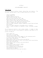
Model Options
RAM requires data on options, sources, meteorology, and receptors.
user must indicate which of the following options are to be used.
-
The
stack-tip downwash
gradual plume rise
buoyancy-induced dispersion
input of point and area sources
emissions from a previous run of RAM
meteorological data on card-image records
input of hourly point and area source emissions
specification of significant point and area sources
input of receptors by specifying coordinates
option for RAM to generate receptors downwind of significant point and
area sources
option for RAM to generate a honeycomb array of receptors
input of radial distances to generate a polar coordinate receptor
array.
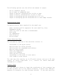
The following are options to omit certain outputs. A number of these
options should be used or the program will generate large quantities of
printed information.
-
point source list
area source list and map
emissions with height table
resultant meteorological data summary for the averaging period
all hourly output (point, area, summaries)
hourly point contribution
meteorological data on hourly point contributions
plume height and distance to final rise on hourly point contributions
hourly area contributions
meteorological data on hourly area contributions
hourly summary
meteorological data on hourly summary
all averaging period output
point averaging period contributions
area averaging period contributions
averaging period summary
average concentrations and high-five table.
5
The following options can also affect the amount of output.
-
use of
use of
output
output
output
output
a default option
parts of segmented runs
of partial concentrations to disk or tape
of hourly concentrations to disk or tape
of averaging period concentrations to a file
of averaging period concentrations to card-image records.
Meteorological Data
The meteorological data required for the model are:
-
power-law wind profile exponents for each stability class
anemometer height
stability class at the hour of measurement
wind speed
air temperature
wind direction
mixing height.
Source Emissions Data
The information required of the emissions sources is:
-
coordinates of the point source
emission rate for sulfur dioxide
emission rate for suspended particulates
physical stack height
stack gas temperature
stack exit diameter
stack gas exit velocity
coordinates of SW corner of area source
side length of area source.
The user may also specify up to 25 point sources and up to 10 area
sources as being significant (i.e., sources for which additional
information is output).
Receptor Data
The user may also choose to input the coordinates of the receptors (up
to 180) or enter one to five radial distances, in which case, RAM will
generate 36 receptors for each distance entered. If the user specifies
6
the array boundaries, RAM can also generate its own honeycomb array of
receptors.
Additionally, RAM can generate receptors downwind of
significant point or area sources if the significant source option is
used.
7
SECTION 3
FEATURES AND LIMITATIONS
USES
RAM is primarily a short-term (one hour to one day) urban or rural
algorithm used to estimate air quality from point and area sources.
Effects of either control strategies or tactics for specific short-term
periods may be examined by users. The expected effect of a proposed
source or sources can also be determined. The spatial variation in air
quality throughout the urban/rural area, or in a portion of the area, for
specific periods can be evaluated readily.
In a forecast or predictive mode such as over a 24-hour period, the
algorithm can assist in locating mobile or portable air samplers and can
assist with emission reduction tactics. Successful use of RAM in the
forecast mode is contingent on the validity of the algorithm assumptions
and the ability to accurately forecast both the input meteorological
parameter values and the input emission parameter values.
The model has the following added features:
-
urban dispersion coefficients recommended by Briggs -- see Figure 7
and Table 8 of Gifford (1976),
wind-profile exponents for urban and rural situations,
optional treatment of calm conditions following methods developed by
the EPA (1984),
stack-tip downwash using the algorithm of Briggs (1974),
momentum-plume rise to treat momentum-dominated plumes as suggested
by Briggs (1969),
buoyancy-induced dispersion following the method of Pasquill (1976),
and a
default option, primarily for regulatory application of the model.
These features were added to satisfy the requirements outlined in
"Guideline on Air Quality Models (Revised)" (EPA, 1986). The default
option is designed as a convenience for the user to help avoid
inadvertent errors in setting the appropriate switches for regulatory
use. The reader is cautioned to refer to the current regulatory guidance
contained in the "Guideline on Air Quality Models".
Urban and Rural Modes
8
The urban dispersion parameter values are those recommended by Briggs and
included in Figure 7 and Table 8 of Gifford (1976). They have been coded
in a subroutine which yields dispersion coefficients as functions of
atmospheric stability and downwind distance. Separate urban and rural
default wind-profile exponents are used in the model. These exponents
are used by the model when the user exercises the default option or when
they have not been provided on input. The rural exponents correspond to
a surface roughness of about 0.1 meters; the urban exponents result from
a roughness of about 1 meter (plus urban heat release influences). For
a more detailed discussion of wind profiles, the reader is referred to
Irwin (1979).
ALGORITHM ASSUMPTIONS
Gaussian Plumes
Calculations of concentrations from point sources are made for emissions
diluted according to the mean wind speed, assuming that the time-averaged
plumes over 1-hour periods have Gaussian (normal) distributions
perpendicular to the plume centerline in the horizontal and vertical.
Narrow Plume Simplification
Calculations of concentrations from area sources are made by considering
that area sources at various distances on a line directly upwind from the
receptor are representative of the sources at those distances that affect
the receptor. This assumption is best fulfilled by gradual rather than
abrupt changes in area emission rates from adjacent area sources. The
narrow plume simplification is considered in more detail in the next
section.
Meteorological Conditions Representative of the Region
The meteorological input for each hour consists of a value for each of
the five parameters: wind direction, wind speed, temperature, stability
class, and mixing height, all of which should be representative of the
entire region containing the sources and receptors. Mixing height is
required only if the atmospheric stability is neutral or unstable.
Steady-state
Calculations are made as if the atmosphere had reached a steady state.
Concentrations for a given hour are calculated independently of
conditions for the previous hour(s).
9
Concentration, Sum of Contributions
The total concentration for a given hour for a particular receptor is the
sum of the estimated contributions from each source.
Vertical Stability
Except for stable layers aloft, which inhibit vertical dispersion, the
atmosphere is treated as a single layer in the vertical with the same
rate of vertical dispersion throughout the
layer. Complete eddy reflection is assumed both from the ground and from
the stable layer aloft given by the mixing layer.
Mixing Height
If vertical temperature soundings are available from a representative
location, they should be used with hourly surface temperatures to
estimate hourly mixing heights for periods with neutral or unstable
stratification. If National Weather Service hourly data are used in the
model, two values of mixing height per day are required. These are the
maximum and minimum mixing heights as defined by Holzworth (1972). The
preprocessor program RAMMET provides a crude interpolation to obtain
hourly mixing heights; however, this interpolation does not consider
hourly surface temperatures.
Wind Speeds and Directions
Wind speeds and directions should be hourly averages (National Weather
Service hourly observations are not really hourly averages, but are
averages of a few minutes at the time of the observation, usually 5 to
10 minutes prior to the hour). Input winds should be representative of
the entire region. In addition to input winds, the user is required to
give the anemometer height.
The increase of wind speed with height is included, based upon a powerlaw wind profile.
The exponent is dependent upon the stability
classification and surface roughness. (See Irwin, 1979.) For any given
hour, winds at various heights above ground are likely to deviate
considerably from this climatological mean profile.
If user-defined
exponents are not supplied, default exponents are used by the model.
There is no inclusion of directional shear with height. This means that
the direction of flow is assumed to be the same at all levels over the
region. The taller the effective height of the emission, the larger the
expected error in the direction of plume transport. Although the effects
of surface friction are such that wind direction usually veers (turns
10
clockwise) with height, the thermal effects (in response to the
horizontal temperature gradient in the region) may cause increased
veering or can overcome the effect of friction and cause backing (turning
counterclockwise with height).
National Weather Service observations report wind to the nearest 10E. In
order to avoid unrealistic results that would occur from having the wind
come from exactly the same direction hour after hour, the program RAMMET,
which processes the meteorological data, uses random numbers from 0 to
9 to add from -4E to +5E to the reported wind direction. The purpose of
this is to prevent an extreme overestimate of concentration at a point
downwind of a source during a period of steady wind when sequential
observations show the same direction.
Rather than allow the plume
centerline to remain in exactly the same position for several hours, the
alteration allows for some variation of the plume centerline within the
10E sector. Although this can in no way simulate the actual sequence of
hourly events (wind direction to 1E accuracy cannot be obtained from wind
direction reported to the nearest 10E), such alterations can be expected
to result in concentrations over a period of record to be more
representative than those obtained using winds to only the 10E increments
reported. (Sensitivity tests of this alteration for single sources have
indicated that, where a few hours of unstable conditions are critical to
producing high concentrations, the resulting concentrations are extremely
sensitive to the exact sequence of random numbers used, such as two wind
directions 1E apart versus two wind directions 9E apart. Differences of
24-hour concentrations from a single source by 40 to 50 percent have
appeared in the sensitivity tests due to the alteration.) It is,
therefore, important to use accurate wind information as input to RAM.
Dispersion Parameter Values
The dispersion parameter values representative for urban areas are those
recommended by Briggs and included in Figure 7 and Table 8 of Gifford
(1976).
The dispersion parameter values representative for open countryside are
the Pasquill-Gifford curves (Pasquill, 1961; Gifford, 1960) which appear
in the Workbook of Atmospheric Dispersion Estimates (Turner, 1970). The
subroutines used to determine the open countryside parameter values are
the same as in the UNAMAP programs MPTER and PTPLU (Pierce and Turner,
1980; Pierce et al., 1982; Chico and Catalano, 1986).
Plume Rise
Plume rise from point sources is calculated using the methods of Briggs
11
(1969, 1971, 1972, 1974, 1975).
Although the plume rise from point
sources is usually dominated by buoyancy, plume rise due to momentum is
also taken into account.
Merging of nearby buoyant plumes is not
considered. Stack-tip downwash is considered, but building downwash is
not.
The variation of effective height of emission from area sources as a
function of wind speed is thought to be an important factor in properly
simulating dispersion in urban areas.
Since this effect is seldom
considered in the compilation of urban area emission inventories, it is
difficult to have the appropriate parameters to estimate this effect;
however, it can be approximated in RAM.
The methodology used is
explained in Section 5.
Emission Inventories
For similar meteorological conditions, the contribution to the
concentration at a receptor from a source is directly proportional to the
emission rate from that source.
It is imperative, therefore, to have
emissions expressed accurately.
Many air pollutant sources vary
emissions with time, such as by hour of the day or weekdays versus
weekends, and attempts should be made to include these variations. For
facilities with detailed emission inventories, hourly emissions can be
determined external to RAM and entered via a separate file. Hourly exit
velocities are calculated within RAM in proportion to annual exit
velocities as hourly emissions are to annual emissions.
Removal or Chemical Reactions
Transformations of a pollutant primarily as a function of time resulting
in loss of that pollutant throughout the entire depth of each plume can
be approximated by RAM. This is accomplished by an exponential decrease
with travel time from the source.
The input parameter is the time
expected to lose 50% (half-life) of the emitted pollutant. RAM does not
have the capability to change this parameter value during a given run.
If the loss to be simulated takes place through the whole plume without
dependence upon concentration, then the exponential loss may provide a
reasonable simulator if the loss rate is realistic. However, if the loss
mechanism is selective, such as impaction with features on the ground,
reactions with materials on the ground, or dependence on the
concentration in a given small parcel of air (requiring consideration of
contributions from all sources to this parcel), the loss mechanism built
into RAM will not be adequate.
Topographic Influences
12
RAM is designed for application over level or gently rolling terrain
where the assumption of a flat plane used in the algorithm is reasonable.
Dispersion parameters for the urban algorithms are representative of
surface roughness over urban areas (zo ~ 1m). Dispersion parameters for
the rural algorithms are representative of surface roughness over rural
The algorithms in RAM have no topographical
areas (zo ~ 0.1 m).
influences incorporated, and some difficulties might be expected in
attempting to use the model in terrain situations.
Under unstable
conditions, plumes may tend to rise over terrain obstructions; under
stable conditions, leveled-off plumes may remain at nearly the same mean
sea level height, but may be expected to alter the plume path in response
to the terrain features, resulting in a different wind direction locally
than that specified for the region.
Fumigation
Fumigation is a transient phenomenon that eliminates the inversion layer
containing a stable plume from below, causing mixing of pollutants
downward and resulting in uniform concentrations with height beneath the
original plume centerline.
This phenomenon is not included in the
calculations made by RAM.
Conditions specified for each hour are
calculated as if a steady state had been achieved.
Default Option
A default option is a feature of the model which facilitates compliance
with regulatory requirements.
For either rural or urban situations,
exercising this option overrides other user-input selections and results
in the following:
-
final plume rise is used (gradual or transitional plume rise is not
used for plume height, but it is used to calculate the magnitude of
the buoyancy-induced dispersion),
buoyancy-induced dispersion is used,
stack-tip downwash is considered,
default urban or rural wind-profile exponents are used as given in
Table 1,
default vertical potential temperature gradients for stable conditions
are used,
a decay half-life of four hours for S02 in urban mode is used,
otherwise no decay,
momentum-plume rise is calculated, and
calms are treated according to methods developed by the EPA (1984).
These are discussed next.
13
Optional Treatment of Calm Conditions
When the default option is exercised, calm conditions are handled
according to methods developed by EPA. A calm hour is indicated in the
preprocessed meteorological data as an hour with a wind speed of 1.0
m/sec and a wind direction the same as the previous hour. When a calm
is detected in the meteorological data, the concentrations at all
receptors are set to zero.
When calculating a multiple-hour average
concentration, the sum of the hourly concentrations is divided by the
number of hours less the number of calm hours, provided that the divisor
used in calculating the average is never permitted to be less than 75
percent of the averaging time being considered. This results in the
following:
-
3-hour averages are always determined by dividing the sum of the
hourly contributions by 3 (i.e., no change from prior methods);
8-hour averages are calculated by dividing the sum of the hourly
contributions by the number of non-calm hours or 6, whichever is
greater;
24-hour averages are determined by dividing the sum of the hourly
contributions by the number of non-calm hours or 18, whichever is
greater; and
period of record averages are calculated by dividing the sum of all
the hourly contributions by the number of non-calm hours during the
period of record.
This calms procedure is not available in RAM outside of the default
option. If not using the default, calms are treated as 1.0 m/s winds.
Summary
The closer the situation to be simulated agrees with the assumptions
stated above, the greater the expectation of reasonable results. The
narrow plume simplification is most reasonable for situations where there
are no great variations in area emission rates for adjacent area sources.
The higher the effective height of a point source, the greater is the
chance for poor results since actual directional shear in the atmosphere,
not included in the algorithm, will cause plumes to move in directions
different from the direction input to the model. Also, the higher the
source height, the greater is the potential for encountering layers in
the atmosphere having dispersion characteristics different from those
being used.
As stated above, it is necessary to properly consider
variations in emissions.
14
Reliable meteorological inputs are also necessary.
The light wind
situation is most likely to violate assumptions, since variations in the
flow over the region are likely to occur, and the slower transport may
cause buildup of pollutants from hour to hour. Unfortunately, these are
the conditions that are likely to be associated with maximum 3-hour and
24-hour concentrations in urban areas. These light wind situations do
not conform to the assumptions of Gaussian steady-state models.
The
calms processing segment in RAM takes into account these deficiencies by
calculating averages for periods longer than three hours in such a way
that persistent light wind conditions do not cause a gross overestimate
of concentrations at a given receptor.
RAM is not appropriate for making concentration estimates for topographic
complications. The greater the departure from relatively flat terrain
conditions, the greater the departure from the assumptions of the
algorithm.
RAM is most applicable for pollutants that are quite stable chemically
and physically. A general loss of pollutant with time can be accounted
for by the algorithm. Selective removal or reaction at the plume-ground
interface or dependence upon concentration levels may not be well handled
by RAM.
15
SECTION 4
BASIS FOR RAM
The basis for RAM is also discussed in Novak and Turner (1976). The user
may select use of either urban or rural parameters. The urban dispersion
parameters Fy and Fz are those suggested by Briggs and reported by Gifford
(1976). The urban F's are functions of distance between source and
receptor and of atmospheric stability class where the class is specified
by open country conditions.
The dispersion parameters for rural conditions are those of PasquillGifford (Pasquill, 1961; Gifford, 1960), as used in the UNAMAP programs
PTPLU, CRSTER, and MPTER. These values are equivalent to the dispersion
parameter values given in Figures 3-2 and 3-3 of the Workbook of
Atmospheric Dispersion Estimates (Turner, 1970).
DILUTION BY THE WIND
Emissions from continuous sources are assumed to be stretched along the
direction of the wind by the speed of the wind. Thus the stronger the
wind, the greater the dilution of the emitted plume. To approximate the
increase in wind speeds with height from point of measurement to stack
top, a power-law increase with height is used. The exponent used is a
function of stability.
DISPERSION RESULTS IN GAUSSIAN-DISTRIBUTED CROSS SECTIONS
The time-averaged concentration distributions through a dispersed plume
resulting from a continuous emission from a point source or an area
element are considered to be Gaussian in both the horizontal and vertical
directions. Modification of the vertical distribution by eddy reflection
at the ground or at a stable layer aloft is considered.
This eddy
reflection is calculated by a "folding back" of the portion of the
distribution that would extend beyond the barrier if it were absent.
This is equivalent to a virtual-image source beneath the ground (or above
the stable layer).
STEADY-STATE CONDITIONS
Concentration estimates are made for each simulated hourly period using
the mean meteorological conditions for that hour as if a steady-state
condition had been achieved. Steady-state Gaussian plume equations are
used for point sources, and the integrations of these equations are used
16
for area sources.
17
SECTION 5
TECHNICAL DESCRIPTION
CONCENTRATION SUM OF INDIVIDUAL CONTRIBUTIONS
The total concentration of a pollutant at a receptor is taken as the sum
of the individual concentration estimates from each point and area source
affecting that receptor, that is, concentrations are additive.
Concentration estimates for averaging time longer than one hour are
determined by linearly averaging the hourly concentrations during the
period.
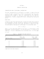
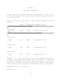
WIND SPEED
In RAM the input wind speed data must include the height above ground of
the measurements, and may include the exponents for the wind profile.
If no exponents are given in the input, the values in Table 1 are used.
The wind speed at the physical stack height h is calculated from:
u(h) = u (h/ha)p
(1)
where u is the input wind speed for this hour, h is the height of wind
measurement, and the exponent p, for the wind profile, is a function of
stability. If u(h) is determined to be less than 1 m/s, it is set equal
to 1 m/s.
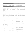
TABLE 1. EXPONENTS FOR WIND PROFILES
44444444444444444444444444444444U
4444444444444444444444444444444444444444444444444444444444444444444444
4
URBAN (RAM)
RURAL (RAMR)
Stability class
exponent
exponent
44444444444444444444444444444444U
4444444444444444444444444444444444444444444444444444444444444444444444
4
A
0.15
0.07
B
0.15
0.07
C
0.20
0.10
D
0.25
0.15
E
0.30
0.35
F
0.30
0.55
4444444444444444444444444444444444444444444U
4444444444444444444444444444444444444444444444444444444444444444444444
PLUME RISE FOR POINT SOURCES
18
The use of the methods of Briggs to estimate plume rise and effective
height of emission are discussed below.
First, actual or estimated wind speed at stack top, u(h), is assumed to
be available.
Stack Downwash
To consider stack downwash, the physical stack height is modified
following Briggs (1973, p. 4). The h' is found from
h' = h + 2{[vs/u(h)] - l.5}d for vs < 1.5 u(h),
(2)
h' = h for vs > 1.5 u (h),
where h is physical stack height (meters), vs is stack gas velocity
(meters per second), and d is inside stack-top diameter (meters). This
h' is used throughout the remainder of the plume height computation. If
stack downwash is not considered, h'= h in the following equations.
Buoyancy Flux
For most plume rise situations, the values of the Briggs buoyancy flux
parameter, F (m4/s3) is needed. The following equation is equivalent to
Briggs' (1975, p. 63) Eq. 12:
F = (g vs d2 )T)/(4 Ts),
(3)
where g is the acceleration of gravity, 9.806 m/s2, )T = Ts - T, Ts is
stack gas temperature (Kelvin), and T is ambient air temperature (Kelvin)
at stack top.
Unstable or Neutral:
Crossover Between Momentum and Buoyancy
For cases with stack gas temperature greater than or equal to ambient air
temperature, it must be determined whether the plume rise is dominated
by momentum or buoyancy. The crossover temperature difference ()T)c is
determined for 1) F less than 55 or 2) F greater than or equal to 55.
If the difference between stack gas temperature and ambient air
temperature, )T, exceeds or equals the ()T)c, plume rise is assumed to be
buoyancy dominated; if the difference is less than ()T)c plume rise is
assumed to be momentum dominated (see below).
The crossover temperature difference is found by setting Briggs' (1969,
p. 59) Eq. 5.2 equal to the combination of Briggs (1971, p. 1031) Eqs.
19
6 and 7 and solving for )T.
For F less than 55,
Ts/d2/3.
(4)
()T)c = 0.00575 vs2/3 Ts/d1/3
(5)
()T)c = 0.0297 vs
1/3
For F equal to or greater than 55,
Unstable or Neutral:
Buoyancy Rise
For situations where )T exceeds or is equal to ()T)c as determined above,
buoyancy is assumed to dominate. The distance to final rise xf (in
kilometers) is determined from the equivalent of Briggs' (1971, p. 1031)
Eq. 7, and the distance to final rise is assumed to be 3.5x*, where x*
is the distance at which atmospheric turbulence begins to dominant
entrainment. For F less than 55,
xf = 0.049 F5/8.
(6)
For F equal to or greater than 55,
xf = 0.119 F2/5.
(7)
The plume height, H (in meters), is determined from the equivalent of the
combination of Briggs' (1971, p. 1031) Eqs. 6 and 7. For F less than 55,
H = h' + 21.425 F3/4/u(h).
(8)
For F equal to or greater than 55,
H = h' + 38.71 F3/5/u(h).
Unstable or Neutral:
(9)
Momentum Rise
For situations where the stack gas temperature is less than the ambient
air temperature, it is assumed that the plume rise is dominated by
momentum. Also if )T is less than ()T)c from Eq. 4 or 5, it is assumed
that the plume rise is dominated by momentum.
The plume height is
calculated from Briggs' (1969, p. 59) Eq. 5.2:
H = h' + 3 d vs/u(h).
(10)
Briggs (1969) suggests that this equation is most applicable when vs/u is
20
greater than 4. Since momentum rise occurs quite close to the point of
release, the distance to final rise is set equal to zero.
Stability Parameter
For stable situations, the stability parameter s is calculated from the
equation (Briggs, 1971, p. 1031):
s = g(M2/Mz)/T
(11)
where 2 is potential temperature. As an approximation, for stability
class E (or 5), M2/2z is taken as 0.02 K/m, and for stability class F (or
6), M2/Mz is taken as 0.035 K/m.
Stable:
Crossover Between Momentum and Buoyancy
For cases with stack gas temperature greater than or equal to ambient air
temperature, it must be determined whether the plume rise is dominated
by momentum or buoyancy. The crossover temperature difference ()T)c is
found by setting Briggs' (1975, p.96) Eq. 59 equal to Briggs' (1969, p.
59) Eq. 4.28, and solving for )T. The result is
()T)c = 0.019582 vs T s1/2.
(12)
if the difference between stack gas temperature and ambient air
temperature ()T) exceeds or equals ()T)c, the plume rise is assumed to be
buoyancy dominated; if )T is less than ()T)c, the plume rise is assumed
to be momentum dominated.
Stable:
Buoyancy Rise
For situations where )T is greater than or equal to ()T)c, buoyancy is
assumed to dominate.
The distance to final rise (in kilometers) is
determined by the equivalent of a combination of Briggs' (1975, p. 96)
Eqs. 48 and 59:
xf = 0.0020715 u(h) s-1/2.
(13)
The plume height is determined by the equivalent of Briggs' (1975, p. 96)
Eq. 59:
H = h' + 2.6{F/[u(h) s]}1/3.
(14)
The stable buoyancy rise for calm conditions (Briggs, 1975, pp. 81-82)
21
is also evaluated:
H = h' + 4 F
1/4
s-3/8
(15)
The lower of the two values obtained from Eqs. 14 and 15 is taken as the
final effective height.
Stable:
Momentum Rise
When the stack gas temperature is less than the ambient air temperature,
it is assumed that the plume rise is dominated by momentum. If )T is
less than ()T)c as determined by Eq. 12, it is also assumed that the plume
rise is dominated by momentum.
The plume height is calculated from
Briggs' (1969, p. 59) Eq. 4.28:
H = h' + 1.5{(vs2 d2 T)/[4 Ts u(h)]}1/3 s-1/6.
(16)
The equation for unstable or neutral momentum rise (10) is also
evaluated.
The lower result of these two equations is used as the
resulting plume height.
All Conditions: Distance Less than Distance to Final Rise (Gradual Rise)
Where gradual rise is to be estimated for unstable, neutral, or stable
conditions, if the distance upwind from receptor to source x (in
kilometers), is less than the distance to final rise, the equivalent of
Briggs' (1971, p. 1030) Eq. 2 is used to determine height:
H = h' + (160 F1/3 x2/3)/u(h).
(17)
This height is used only for buoyancy-dominated conditions; should it
exceed the final rise for the appropriate condition, the final rise is
substituted instead.
General
In working through the receptors to determine concentrations for a given
hour, the first time a source is found to lie upwind of a receptor, the
following quantities are determined and stored for that source: u(h),
h', F, H, and xf. These quantities are then used each time this source
is encountered during this hour without recalculation.
Only if the
upwind receptor-source distance is less than xf is the effective plume
height determined for each occurrence by the last equation mentioned.
22
BUOYANCY-INDUCED DISPERSION FOR POINT SOURCES
For strongly buoyant plumes, entrainment as the plume ascends through the
ambient air contributes to both vertical and horizontal spread. Pasquill
(1976) suggests that this induced dispersion, Fzo, can be approximated by
the plume rise divided by 3.5.
Fzo = )h/3.5
(18)
where )h is either the gradual plume rise as calculated by Eq. 5 for
distances less than the distance to final rise, or the final rise for
distances greater than that distance. The effective dispersion can then
be determined by adding variances:
Fze = (Fzo2 + Fz2)1/2,
(19)
where Fze is the effective dispersion, and Fz is the dispersion due to
ambient turbulence levels. At the distance of final rise and beyond, the
induced dispersion is constant, based on the height of final rise. At
distances closer to the source, gradual-plume rise is used to determine
the induced dispersion.
Since in the initial growth phases of release, the plume is nearly
symmetrical about its centerline, buoyancy-induced dispersion in the
horizontal direction, Fyo, equal to that in the vertical direction, is
used,
Fyo = )h/3.5
(20)
To yield an effective lateral dispersion value, Fye, this expression is
combined with that for dispersion due to ambient turbulence:
Fye = (Fyo2 + Fy2)1/2.
(21)
EFFLUENT RISE FOR AREA SOURCES
RAM can include in effective height with wind speed for area sources.
The input area source height, HA, is assumed to be the average physical
height of the area source plus the effluent rise with a wind speed of 5
m/s.
The user specifies the fraction, f, of the input height that
represents the physical height, hp. This fraction is the same for all area
sources in the inventory.
hp = f HA
23
(22)
The difference is the effluent rise for a wind speed of 5 m/s
)H (u = 5) = HA - hp
(23)
If f = 1, there is no rise and the input height is the effective height
for all wind speeds. For any wind speed, u, the rise is assumed to be
inversely proportional to wind speed and is determined from:
)H (u) = 5(HA - hp) / u
(24)
and the effective height is:
He (u) = hp + )H(u).
(25)
CONCENTRATION FORMULAS
Concentrations from Point Sources
The upwind distance x of the point source from the receptor and the
crosswind distance, y, of the point source from the receptor are
calculated as part of estimates for each source-receptor pair for each
simulated hour. Both dispersion parameter values Fy and Fz are determined
as functions of this upwind distance x and stability class.
The terms below are used in the equations that follow.
g1 = exp (-0.5y2/Fy2)
g2 = exp [-0.5(z - H)2/Fz2] + exp [-0.5(z + H)2/Fz2]
4
g3 = E {exp [-0.5(z - H + 2NL)2/Fz2] +
N=-4
exp [-0.5(z + H + 2NL)2/Fz2]}
(This infinite series converges rapidly and evaluation with N varying
from -4 to +4 is usually sufficient.) where
H
= effective height of emissions, meters
L
= mixing height, the top of the unstable layer, meters
y
= crosswind distance, meters
z
= receptor height above ground, meters
24
Fy = standard deviation of plume concentration distribution in
the horizontal, meters
Fz = standard deviation of plume concentration distribution in
the vertical, meters
One of three equations is used to estimate concentrations under various
conditions of stability and mixing height. The equation
Pp = Qg1g2 / (2BFyFzu)
(26)
is used for stable conditions or for unlimited mixing where,
Pp
=
Q
=
ground-level concentration from a single point source,
g/m3, and
point source emission rate, g/sec.
In this equation, eddy reflection at the ground is assumed. For unstable
or neutral conditions where vertical dispersion is great enough that
uniform mixing is assured (Fz > 1.6L) beneath an elevated inversion, the
following equation is used.
Pp = Qg1 / FyLu(2B)1/2
(27)
(If H or z is above the mixing height, Pp = 0.)
For unstable or neutral conditions where uniform mixing is not assured
(Fz<1.6L), the following equation is used.
Pp = Qg1g3 / (2BFyFzu)
(28)
This equation incorporates multiple eddy reflections from the ground and
the base of the stable layer aloft.
Concentrations from Area Sources
The total concentration at a receptor from the two-dimensional area
source distribution is calculated using the narrow plume simplification
discussed by Gifford and Hanna (1971). This simplification is assumed
because the upwind zone of influence affecting a receptor (an upwind
oriented point source plume) is normally quite narrow in comparison with
the characteristic length scale for appreciable changes in the magnitude
of the area-source emission rate itself. Under these circumstances the
two-dimensional
integral
that
expresses
the
total
area-source
contribution to concentration at a receptor can be replaced approximately
25
by a one-dimensional integral.
This integral involves only:
-
knowledge of the distribution of the area-source emission rates along
the line in the direction of the upwind azimuth from the receptor
location,
-
the meteorologically dependent function that specifies the crosswindintegrated concentration in the Gaussian plume from a point source.
In using this area source technique, Gifford and Hanna assumed areasource emissions at ground level, allowing integration upwind to be
accomplished analytically. In RAM the area sources are allowed to have
an effective height, requiring the integration to be accomplished
numerically. Internal tables of integrations for one to three effective
area source heights are calculated at the beginning of each simulated
hour using the specific meteorological conditions for that hour. The
total concentration from all area sources is determined by performing the
integration piecewise over each source in the upwind direction from the
receptor until the farthest boundary of the source region is reached.
26
SECTION 6
VERIFICATION RUN
A sample input data set and the resulting output are distributed with the
model code for verification purposes. A detailed discussion of that data
set can be found in Section 6 of the complete "User's Guide for RAM"
which is available from NTIS.
27
SECTION 7
USES OF RAM
RAM simulates pollutants from point and area sources in urban or rural
settings over periods of one hour to one year. The meteorological data
can be entered on cards, with one card for each simulated hour, or on
magnetic media by using option 8. General emission information can also
be on the input stream or from disk or tape files using option 9 or 10.
Point and area sources are specified by options 5 and 6.
of receptors may be specified by the user (option 14).
The locations
The use of options 15 and 16 to locate additional receptors downwind of
significant point and area sources assists in determining locations of
maximum concentration. Since the resultant wind vector for the averaging
period selected is used to determine the direction of these receptors
from the sources, averaging times that contain significant wind shifts
may result in misleading averages.
The user should note that when
options 15 and 16 are used to locate receptors downwind from significant
sources, the locations for these receptors will shift for each averaging
period, dependent upon the resultant meteorological conditions for each
period. Therefore, receptors with the same numbers will be at different
locations for different averaging times.
If the user desires to cover a specific area so that pollutant patterns
are discerned, option 17 can be used to place additional receptors. The
pattern used is such that adjacent receptors are equidistant; this is
referred to as a honeycomb pattern. The distance between receptors is
selected by the user as are the boundaries of the area covered. If the
boundaries are entered as zeros, the boundaries are set to coincide with
the boundaries of the area source map array.
Since the honeycomb
receptors are set for each averaging time, they may be different from one
averaging time to another. The model can be executed for an hour without
receptors downwind of significant sources in order to obtain a list of
receptors for good area coverage. Their coordinates can then be input
for a longer period run where it is desired to have receptors in fixed
positions.
It should be noted that concentration gradients may be very steep,
especially those due to point source plumes. Therefore, the addition of
more receptors will result in a more complex concentration pattern and
some hot spots. The user, when searching for maximum concentrations,
must decide on receptor spacing commensurate with resources, analysis
28
time, and the
receptors.
purpose
of
the
project
before
including
additional
For the typical run, hourly output would be desired, so option 24 should
be set for hourly output. If option 24 is not set, no hourly output is
printed. The use of option 40 to write partial concentrations onto a
disk file should be used only if additional computer analysis is intended
using the individual contributions of sources upon particular receptors.
Computer programs to perform this analysis must be written by the
individual user to suit his or her purpose.
Option 30 is checked only if option 24 is used to obtain hourly
summaries. The use of option 30 will print a summary page for each hour.
This summary provides the total concentration for each receptor, the
contribution to the concentration from all point sources, the
contribution to the concentration from all area sources, the contribution
from all the significant point sources combined, and the contribution
from all the significant area sources. Information that will be obtained
by using option 24, but not option 30, are the contributions to the
concentrations at each of the receptors from each of the significant
sources.
The maximum of 10 significant area sources results in an
additional page of output per simulated hour.
The maximum of 25
significant point sources results in three additional pages of output per
simulated hour (one page for every 10 significant point sources or
fraction thereof).
Unless the concentration contributions are
specifically needed for analysis of contributions from particular
sources, option 30 should be zero to reduce the quantity of output.
Option 8 would be set to one to enter meteorological data as part of the
run stream rather than reading an external file using unit 11. Options
9 and 10 are set to one to enter hourly emissions. If the contribution
at a receptor from particular sources is of interest, and if these
particular sources are not high enough to be included in the significant
source list from RAM, options 11 and 12 may be used to specify the
sources of interest. If option 11 or 12 is used to obtain concentration
contributions for the averaging time, it is desirable to leave option 30
off to obtain hourly output.
Option 41 or 42 would not usually be employed unless concentrations at
each receptor are required for further analysis or are to be used with
graphics software to produce concentration isopleth maps.
29
SECTION 8
COMPUTER ASPECTS OF THE MODEL
STRUCTURE OF RAM
RAM consists of three sections:
and output subroutines.
preprocessing subroutines, main logic,
Inputs for the model are assumed to be from disk files; outputs either
go to disk or printer. Options and program control are read from FORTRAN
unit 5; processing is then controlled through specifications in this
file. If so specified in the control file, meteorology and emissions can
be obtained from units 11, 15, and 16, respectively. The program uses
two temporary files for intermediate work, but they are not temporary in
the JCL sense, i.e., they are not deleted at the end of the job step and
should be deleted by the user when they are no longer needed. As the
program calculates concentrations, they are averaged and written to units
1, 10, 12, and 13. Tabular output is written to unit 6 which is usually
the default for printed files.
Preprocessing subroutines are used to initialize variables and are called
to determine dispersion parameter values as functions of stability class
and source-receptor distance. The data produced are coefficients and
exponents for the various ranges of effective height of emission and are
used to determine maximum Pu/Q (relative concentration normalized for
wind speed) for point sources and distance to maximum concentration for
point and area sources as functions of stability class and effective
height of emission.
Other subroutines process the emission data. Their principal task is to
set up the area source map array. The area source map array provides
correspondence between locations (referred to by coordinates) and area
source number. Other tasks, such as ranking sources according to set
criteria, are also accomplished.
RAM expects hourly meteorological input data, including mixing height and
stability class.
This and other values can be entered in the input
stream or from a preprocessed file. The auxiliary program RAMMET can
process raw meteorological data into the needed format using hourly
surface data and mixing heights from the National Climatic Data Center.
Input consists of one year of surface data (one observation per hour) and
one maximum and one minimum mixing height per day. RAMMET determines
hourly stability and performs interpolations to estimate hourly mixing
30
heights. The output data are organized to produce a single record for
each day.
The output subroutines are OUTPUT and OUTAV.
OUTPUT provides hourly
concentrations in micrograms per cubic meter, including the contributions
from significant point sources along with a summary table.
OUTAV
provides the same information for the averaging period.
PROGRAM MODULES
After initialization, the flow is governed by three loops:
calendar
days, averaging time, and hours. A minimum of one hour and a maximum of
8,784 hours can be processed by the model. A brief description of the
main program and subroutines follows.
MAIN -
The main program determines Pu/Q maxima and distance to the
point of maximum for point sources as functions of stability
class and effective height of emissions.
Coefficients and
exponents relating these two parameters to effective height of
emission are determined for various stability and effective
height range combinations. These coefficients and exponents, as
well as ones for determining the distance of the maximum
concentration downwind from the edge of an area source, are
calculated for use in the emissions module which processes
emission inventory information for later use.
An important
aspect of this is the construction of the area source map array
which allows a correspondence between any location in the area
source region and the number of the area source at that
location.
All source coordinates in units convenient to the
user (user units) are converted to internal units. An internal
unit is a length such that any area source side length used in
a given run can be expressed as an integer multiple of an
internal unit.
The internal unit is generally equal to the
length of the side of the smallest area in the emission
inventory. The user must determine the internal unit length and
specify it in user units.
Both point and area sources are
ranked according to expected impact at ground level. The 25
point sources and the 10 area sources with the greatest expected
ground-level impact are listed. Also, the total emissions from
various physical heights for both point and area sources are
listed. This helps the user in determining area source heights
and the number to be used.
BRIEF DESCRIPTION OF SUBROUTINES
31
The subroutine and function descriptions that follow are called by RAM
to perform specific tasks.
ANGARC -
This function determines the appropriate arctan of the east
resultant wind component over the north resultant wind
component with the resulting angle between 0E and 360E
JMHREC -
This subroutine and entry point GREC called by RAM determine
receptor locations downwind of significant sources based upon
the resultant meteorological conditions for the averaging
period, usually 3 or 24 hours.
Plume rise and effective
height of emission are calculated.
The distance of the
maximum concentration is determined as a function of the
stability and the effective height of emission in order to
locate the position of a receptor.
Two receptors are
generated for each significant point source, one at the
expected distance of maximum concentration and one at twice
this distance. One receptor is generated for each significant
area source at the expected distance of maximum concentration.
JMHHON -
This subroutine called by RAM generates additional receptors
within a specified area in order to give adequate coverage of
that area with the minimum number of receptors. Receptors are
placed equidistant from nearby receptors, resulting in a
honeycomb array. The distance between receptors is an input
to the main program.
Proposed honeycomb receptors located
closer than half this distance to any other receptor are not
included.
PT -
This subroutine calculates concentrations from point sources.
Subroutines RCON and SYZ (ENTRY point in SYSZ) are called to
complete the computations.
RCON -
This subroutine called by PT calculates P/Q, the relative
concentrations from point sources. This subroutine calls SYZ.
SYZ -
JMH54 -
This subroutine called by RCON calculates the standard
deviation of the concentration in the y- and z- directions.
It employs the Briggs urban dispersion parameters for urban
conditions, and the Pasquill-Gifford parameters for rural
conditions.
This subroutine called by RAM generates tables of Pu/qA (relative
concentration normalized for wind speed) from area sources that
extend from a receptor to various upwind distances. A table is
32
produced for each area source height. One to three heights can
be used. This subroutine calls subroutine JMHCZ.
JMHCZ - This subroutine called by JMH54 calculates concentrations from
infinite crosswind line sources at a distance x upwind from a
receptor. To obtain the vertical dispersion parameter value Fz,
subroutine SIGZ is called.
SIGZ -
This subroutine called by JMHCZ determines the value of the
vertical dispersion parameter Fz for a given upwind distance of
a receptor to the source. The parameter values for urban areas
are those put into equation form by Briggs.
The parameter
values for rural areas are from Pasquill-Gifford.
JMHARE -
This subroutine performs the integration along the line upwind
from the receptor to obtain the effect of all area sources
along the line. This is accomplished by finding the nearest
and farthest distance of each source along the path and
calling subroutine JMHPOL for each distance.
JMHPOL -
This subroutine called by JMHARE interpolates for a given
distance from the values in the tables generated by subroutine
JMH54. This yields the effect of an area source at the given
height extending upwind to this distance.
RANK -
This subroutine arranges concentrations of various averaging
times into tables of the highest five concentrations for each
receptor for each averaging time (high-five tables).
OUTPT -
This subroutine produces output concentrations in micrograms per
cubic meter for each hour for significant sources and for the
summaries.
OUTAV - This subroutine called by RAM gives concentrations for the
averaging period. Contributions and/or summary information are
also generated by OUTAV.
PROCESSOR PROGRAM RAMMET
If option 8 specifies that meteorological data should be expected from
a file, a peripheral program RAMMET can be used to generate the file.
RAMMET processes meteorological data for one year.
The data input
consists of hourly meteorological records in the standard card format 144
of the National Climatic Data Center and twice-a-day estimates of mixing
height (minimum and maximum). Hourly stability class is determined using
33
the objective method of Turner (1964) based on Pasquill's technique
(Pasquill, 1961). Shifts by only one stability class are allowed for
adjacent hours. Hourly mixing height is interpolated from the twice-aday estimates. Hourly meteorological data of wind direction, wind speed,
temperature, stability class, and mixing height are written into a file
with one record per day for the entire year. Random numbers can be read
from a file or generated by the computer used.
34
SECTION 9
INPUT DATA PREPARATION
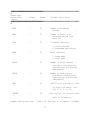
In this section, the general input data requirements are listed. There
are 18 record types in the input stream. Each record type consists of
one or more records.
Table 2 describes the input data; in some cases an explanation follows
the entry.
TABLE 2. RECORD INPUT SEQUENCE FOR RAM
4444444444444444444444444444444444444U
4444444444444444444444444444444444444444444444444444444444444444444444
4
Record type
and variable
Column
Format
Variable description
Units
4444444444444444444444444444444444444444444444444444U
4444444444444444444444444444444444444444444444444444444444444444444444
4
Record type 1
LINE1
---
1-80
20A4
80-character title
1-80
20A4
80-character title
1-80
20A4
80-character title
Record type 2
LINE2
--Record type 3
LINE3
---
RECORDS 1 - 3. Each card image has up to 80 alphanumeric characters.
The input title appears on all output and can suit the user. Normal use
has been to identify the user and run date on card-image 1, the location
and date of the emissions data on card-image 2, and the location and
dates of both surface and upper-air meteorological data on card-image 3.
RAM-RECORD TYPE 4 - 14 variables
Record type 4
35
IDATE(1)
---
FF*
---
2-digit year
IDATE(2)
---
FF
Starting Julian day
IHSTRT
---
---
FF
Starting hour
*FF is free format.
36
---
44444444444444444444444444444444U
4444444444444444444444444444444444444444444444444444444444444444444444
4
Record type
and variable
Column
Format
Variable description
Units
44444444444444444444444444444444U
4444444444444444444444444444444444444444444444444444444444444444444444
4
NPER
---
FF
Number of averaging
periods
NAVG
---
FF
Number of hours in an
--averaging period (commonly 24)
IPOL
---
---
FF
Pollutant indicator
MUOR
---
---
NSIGP
---
FF
Number of point sources --from which concentration
contributions are desired
(maximum=25)
NSIGA
---
FF
Number of area sources --from which concentration
contributions are desired
(maximum=10)
NAVS
---
---
FF
Additional averaging time
CONONE
---
---
---
3, sulfur dioxide
4, suspended particulate
FF
Model indicator
1, urban mode
2, rural mode
for high-five table.
ally 2, 4, 6, or 12.
Example multipliers are:
FF
Multiplier
Usu-
to convert user
units to kilometers.
3.048 x 10-4 for feet to kilometers; 1.609347
37
for miles to kilometers; 1.0 x l0-3 for meters to kilometers.
UNITS
---
---
Z
---
m
FF
Number
of
user units per
smallest area source side
length. Should equal 1
if no area sources.
(internal units)
FF
Receptor height
38
44444444444444444444444444444444U
4444444444444444444444444444444444444444444444444444444444444444444444
4
Record type
and variable
Column
Format
Variable description
Units
44444444444444444444444444444444U
4444444444444444444444444444444444444444444444444444444444444444444444
4
HAFL
sec
An entry of zero
calculations.
--in
FF
HAFL
will
Pollutant half-life
cause
RAM
to
skip
pollutant
loss
RAM-RECORD TYPE 5 - The values are for 50 different options; 1 is used
to employ the option and a zero indicates non-use.
Record type 5
IOPT(1)
---
1
I1
No stack downwash
IOPT(2)
---
2
I1
No gradual plume rise
IOPT(3)
---
3
I1
Use buoyancy induced
IOPT(4)
4
I1
Not used
---
IOPT(5)
---
5
I1
Input point sources
IOPT(6)
---
6
I1
Input area sources
IOPT(7)
---
7
I1
Use
IOPT(8)
---
8
dispersion
emissions from previous
run. Data accessed from
Unit 9.
I1
Meteorology
39
data in input
stream. Otherwise, input
from Unit 11.
IOPT(9)
---
9
I1
Read
hourly point source
IOPT(10)
10
I1
Read hourly area source --emissions (Unit 16)
IOPT(11)
---
11
I1
Specify significant point
emissions (Unit 15)
sources
Option 11 will allow the examination of the individual contributions to
each receptor from each of the specified sources. Both point and area
sources may be specified. (See IOPT(12).)
40
44444444444444444444444444444444U
4444444444444444444444444444444444444444444444444444444444444444444444
4
Record type
and variable
Column
Format
Variable description
Units
44444444444444444444444444444444U
4444444444444444444444444444444444444444444444444444444444444444444444
4
IOPT(12)
---
12
I1
Specify significant area
IOPT(13)
13
I1
---
Not used
IOPT(14)
14
I1
Enter receptors by
--specifying coordinates
IOPT(15)
15
I1
RAM generates receptors --downwind of significant
point sources
IOPT(16)
---
16
I1
RAM generates receptors
IOPT(17)
---
17
sources
downwind of significant
area sources
I1
RAM generates honeycomb
array of receptors to
cover specified area
RAM generates a honeycomb array of receptors, placed equidistant in
staggered rows over a specified area. This insures good area coverage.
Candidate receptor positions are checked against other receptors (either
input or generated by other options of the program) and if the distance
between the proposed receptor is less than one-half the normal distance
between honeycomb receptors, then the candidate receptor is not added to
the list. The boundaries of the area to be covered by these receptors
are specified by the user.
IOPT(18)
---
18
I1
Input radial distances
to generate polar
coordinate receptor array.
41
36 receptors for each
distance.
IOPT(19)
19
I1
Not used
---
Printed output is controlled by the options that follow. Options 20
through 36 are all options to omit output. In the program default, most
of these options to omit output are used since some of the options can
generate large amounts of printed output.
42
44444444444444444444444444444444U
4444444444444444444444444444444444444444444444444444444444444444444444
4
Record type
and variable
Column
Format
Variable description
Units
44444444444444444444444444444444U
4444444444444444444444444444444444444444444444444444444444444444444444
4
IOPT(20)
20
I1
Omit point source list
IOPT(21)
---
21
I1
Omit
IOPT(22)
---
22
IOPT(23)
---
23
IOPT(24)
24
I1
Omit all hourly output --(point, area, summaries)
IOPT(25)
---
25
I1
Omit
IOPT(26)
---
26
IOPT(27)
---
27
IOPT(28)
---
28
IOPT(29)
29
area
---
source list and
map
I1
Omit
emissions with height
table
I1
Omit resultant meteorology
data summary for averaging
period
hourly point contribu-
tions
I1
Omi t
meteorology data on
hourly point contributions
I1
Omit plume height and
distance to final rise
on hourly point contribution
I1
Omit hourly area
contributions
I1
O mit
43
meteorology data on
---
hourly area contributions
IOPT(30)
---
30
I1
Omit hourly summary
IOPT(31)
---
31
I1
Omit
IOPT(32)
---
32
IOPT(33)
---
33
meteorological data on
hourly summary
I1
Omit
all averaging period
output
I1
Omit
point averaging period
contributions
44
44444444444444444444444444444444U
4444444444444444444444444444444444444444444444444444444444444444444444
4
Record type
and variable
Column
Format
Variable description
Units
44444444444444444444444444444444U
4444444444444444444444444444444444444444444444444444444444444444444444
4
IOPT(34)
---
34
IOPT(35)
---
35
IOPT(36)
---
36
IOPT(37)
37
I1
Omit
area averaging period
contributions
I1
Omit averaging period
summary
I1
Omit average concentrations
and highest five concentrations table
I1
---
Not used
The remaining options control the flow of the program and the amount of
output. This is especially so for Option 40, in which a large file can
be generated by employing this option.
IOPT(38)
38
I1
Set default option for --regulatory application
Option 38 sets a series of options and parameters when the model is to
be used for regulatory application.
IOPT(39)
---
39
I1
Part of segmented run
IOPT(40)
---
40
I1
Write partial concentrations to disk or tape
(Unit 10)
The user will need to write the software to process this output.
Although it is unlikely that Options 39 and 40 will be employed on the
same run, it is possible to do so. However, the second and subsequent
45
segments will not skip over previously generated partial concentration
files.
Therefore, unless Unit 10 accesses a different file on each
segment, any previously generated partial concentration files will be
overwritten.
46
44444444444444444444444444444444U
4444444444444444444444444444444444444444444444444444444444444444444444
4
Record type
and variable
Column
Format
Variable description
Units
44444444444444444444444444444444U
4444444444444444444444444444444444444444444444444444444444444444444444
4
IOPT(41)
---
41
IOPT(42)
42
I1
Write hourly concentrations
to disk or tape (Unit 12)
I1
Write averaging-period --concentration to disk
or tape (Unit 13)
The output files generated by Options 41 and 42 are useful only when the
receptors are set for the run and not varying from one averaging period
to another. Therefore, these options can be used with Options 14 and 18,
but a program termination will occur in trying to use Option 41 or 42 in
combination with any of Options 15, 16, or 17.
IOPT(43)
43
I1
Write averaging-period --concentrations in cardimage format (80 bytes)
to Unit 1.
IOPT(44)
---
44
I1
Not used this version
IOPT(45)
---
45
I1
Not used this version
IOPT(46)
---
46
I1
Not used this version
IOPT(47)
---
47
I1
Not used this version
IOPT(48)
---
48
I1
Not used this version
IOPT(49)
---
49
I1
Not used this version
47
IOPT(50)
---
50
I1
Not used this version
RAM-RECORD TYPE 6 - 2 variables, 1 to 7 values. Selection of the default
option (Option 38) causes wind exponents to be set to the default values
for the appropriate urban or rural cases. This record is still required
to input the anemometer height; all other data on the record will be
ignored when Option 38 is set.
Record type 6
HANE
---
FF
Anemometer height
PL(I)
---
FF
Wind speed power law
exponents
48
m
---
44444444444444444444444444444444U
4444444444444444444444444444444444444444444444444444444444444444444444
4
Record type
and variable
Column
Format
Variable description
Units
44444444444444444444444444444444U
4444444444444444444444444444444444444444444444444444444444444444444444
4
RAM-RECORD TYPE 7 - 9 variables, 8 values (one of these records for each
point source).
This is used if Option 5 = 1 (the user inputs point
sources) and Option 7 = 0 (no emissions are entered from a previous run).
Record type 7
PNAME(I,NPT)
---
1-12
SOURCE(1,NPT)
---
13-20
SOURCE(2,NPT)
---
21-28
SOURCE(3,NPT)
g/sec
29-36
3A4
12-character point source
identification
F8.2
East coordinate of point
source (user units)
F8.2
North coordinate of point
source (user units)
F8.2
Sulfur dioxide emission
rate
Emission rates for pollutants other than sulfur dioxide and particulates
may be substituted.
If substitutions are made, changes in data
statements are necessary in order to have the proper pollutant names on
the printed output.
SOURCE(4,NPT)
g/sec
37-44
F8.2
Particulate emission rate
SOURCE(5,NPT)
m
45-52
F8.2
Physical stack height
SOURCE(6,NPT)
K
53-60
F8.2
Stack gas temperature
SOURCE(7,NPT)
61-68
F8.2
Stack inside diameter
49
m
SOURCE(8,NPT)
m/sec
69-76
F8.2
Stack gas exit velocity
To indicate the end of point source records, the word "ENDP" is placed
in record columns 1 to 4.
RAM-RECORD TYPE 8 - 7 variables, 6 values (one of these records is
required for each area source). This is used if Option 6 = 1 (the user
inputs area sources) and Option 7 = 0 (no emissions input from previous
run).
50
44444444444444444444444444444444U
4444444444444444444444444444444444444444444444444444444444444444444444
4
Record type
and variable
Column
Format
Variable description
Units
44444444444444444444444444444444U
4444444444444444444444444444444444444444444444444444444444444444444444
4
Record type 8
ANAME(J,NAS)
---
1-12
3A4
12-character area source
13-22
F10.2
East coordinate of SW
identification
ASORC(1,NAS)
---
corner
of area source
(user
units)
ASORC(2,NAS)
---
23-32
ASORC(5,NAS)
---
33-42
F10.2
North coordinate of SW
corner of area source
(user units)
F10.2
Side
length
of area source
(user units)
Note that ASORC(5,NAS) - side length, is read out of order to conform
with the existing order of IPP emissions data.
ASORC(3,NAS)
g/sec
43-52
ASORC(4,NAS)
g/sec
53-62
F10.2
Sulfur dioxide emission
rate for entire area
F10.2
Particulate emission rate
for
entire area
Particulate Emission Rate for entire area is a total rate for the entire
area. It is later transformed into gm/sec-1m-2. As with point sources,
51
emission rates for other pollutants may be substituted for sulfur dioxide
and particulates, with appropriate name changes made in the data
statements to modify titles on the printouts.
ASORC(6,NAS)
63-72
F10.2
Area source height
m
Although only one pollutant can be considered for a given run of RAM,
both of the entered emission rates are listed in the output. One of the
emission rates may be left off and will appear as zeros in the output.
Area sources can vary in size, but certain requirements must be met.
There must be a definable internal unit such that the side length of all
other area sources is an integer multiple of the side length of this
internal unit. For example, if an emission inventory consists of area
source squares having side lengths of 1, 2.5, 5, and 10 km, the internal
unit must be chosen to equal 0.5 km. It is better to conduct emission
inventories so that area source squares have side lengths that are
multiples
of
the
side
lengths
of
the
smallest
area
source
44444444444444444444444444444444U
4444444444444444444444444444444444444444444444444444444444444444444444
4
Record type
and variable
Column
Format
Variable description
Units
44444444444444444444444444444444U
4444444444444444444444444444444444444444444444444444444444444444444444
4
squares. Also, if a grid is constructed of unlt squares, squares having
side length of one internal unit, the boundaries of all area sources must
coincide with lines ln that grid; there can be no overlap of one area
source over another. Although these statements may seem restrictive, the
area source entries to RAM are quite versatile. Concentrations from area
sources are calculated by performing computations for each area source
encountered in proceeding from a receptor in the upwind direction until
the upwind boundary of the area source is encountered. If there are
large areas (larger than the unit square) of zero emissions within the
rectangle that includes all area sources (area source region), it is
desirable to define these as area sources with zero emissions in squares
as large as possible.
This will result in considerable savings in
computer processing time.
If the height of emission is the effective height of the area source at
a wind speed of 5 m/sec, and if the physical height of the source is a
set fraction of this value, which is the same for all area sources, it
will be possible to consider the variation of effective height of area
sources with wind speed in RAM. Otherwise, the fraction will be 1.0 and
52
it will be assumed that the input height of emission is the effective
height for all wind speeds.
RAM-RECORD TYPE 9 - 2 variables. This record is required only if Option
11 is used (i.e., the user will specify significant point sources).
Record type 9
INPT
1-3
---
I3
Number of user-specified
significant sources
The maximum number of user-specified significant point sources is 25 this number must be non-zero.
MPS(I)
4-78
---
I3
INPT point source numbers
the
user wants considered
significant (max = 25)
There will be as many sources in this list as indicated in INPT.
RAM-RECORD TYPE 10 - 4 variables - 4 values.
Information for area
sources. This record is required only if Option 6 is employed (user will
input area sources).
53
44444444444444444444444444444444U
4444444444444444444444444444444444444444444444444444444444444444444444
4
Record type
and variable
Column
Format
Variable description
Units
44444444444444444444444444444444U
4444444444444444444444444444444444444444444444444444444444444444444444
4
Record type 10
FH
---
XLIM
---
FF
Fraction of area source
height which is physical
height
---
FF
Distance limit on inte- --gration for area source
(user units)
The distance XLIM should be equal to or exceed the greatest possible
distance from a receptor (including receptors generated by RAM) to the
farthest corner of the area source region for this run, but cannot exceed
116 kilometers.
NHTS
---
---
HINT
m
---
FF
Integer
number of heights
to be used for area
sources (min=1, max=3)
FF
Height(s)
for area source
integrations. Same
number as NHTS.
RAM-RECORD TYPE 11 - 1 variable - 1 or 2 values.
only if record type 10 is used.
This record is required
Record type 11
BPH
m
---
FF
Breakpoint heights between
area source heights
These values are to be used as boundaries between the specified area
source heights used for calculations. If only one area source height is
54
to be used, only one BPH value is entered; it should be greater than any
area source height of the area source data. If NHTS is 2, the single
value for BPH should be between the two HINT values. If NHTS is 3 and
the three HINT values are, for example, 15, 25, and 35; the two values
for BPH might be 20 and 30.
RAM-RECORD TYPE 12 - 2 variables - 1 to 11 values.
This record is
required only if Option 12 is used (i.e., user specifies significant area
sources).
55
44444444444444444444444444444444U
4444444444444444444444444444444444444444444444444444444444444444444444
4
Record type
and variable
Column
Format
Variable description
Units
44444444444444444444444444444444U
4444444444444444444444444444444444444444444444444444444444444444444444
4
Record type 12
INAS
---
1-3
MAS
---
4-33
I3
Number of user-specified
significant area sources
(max=10)
I3
INAS
area so urce numbers
the user wants to
consider significant
RAM-RECORD TYPE 13 - 4 variables.
data will be input on Unit 11).
Used if Option 8 = 0 (meteorological
Record type 13
ISFCD
---
---
FF
Surface Met. Station
Identifier
ISFCD is a 5-digit identification of the meteorological tape to be used.
For tapes generated by the National Climatic Data Center, this will
normally be the surface station number.
ISFCYR
---
FF
Year of surface meteorology data
IMXD
---
FF
Upper-air Station
Identifier
---
IMXYR
---
FF
Year of mixing height
data (2 digits)
---
56
44444444444444444444444444444444U
4444444444444444444444444444444444444444444444444444444444444444444444
4
Record type
and variable
Column
Format
Variable description
Units
44444444444444444444444444444444U
4444444444444444444444444444444444444444444444444444444444444444444444
4
RAM-RECORD TYPE 14 - 3 variables - 7 values. This record is used with
Option 18 (input of polar coordinates) if the user chooses to input
receptor positions according to a radial distance from a coordinate
source.
Record type 14
RADIL(I)
---
FF
One to five radial dis- --tances (user units)
RADIL(I) is one to five radial distances (with the remaining distances
entered as zeros) centered on any location.
Each radial distance
generates 36 receptors at each radial distance at azimuths of 10 to 360
degrees.
CENTX
---
FF
East coordinate about
--which radials are
centered (user units)
CENTY
---
FF
North coordinate about --which radials are centered (user units)
RAM-RECORD TYPE 15 - 3 variables. If Option 14 (user specifies receptor
coordinates) is used, there will be one record for each receptor that the
user specifies.
Record type 15
RNAME(I)
1-8
2A4
8-digit alphanumeric
--station identification
RREC
9-18
F10.3
East coordinate of
--receptor (user units)
SREC
19-28
F10.3
North coordinate of
receptor (user units) ---
57
Both coordinates of receptors should be positive.
Receptors may be
either inside or outside the area source region. A record with "ENDR"
in columns 1 - 4 signals that the receptor list has been completed.
58
44444444444444444444444444444444U
4444444444444444444444444444444444444444444444444444444444444444444444
4
Record type
and variable
Column
Format
Variable description
Units
44444444444444444444444444444444U
4444444444444444444444444444444444444444444444444444444444444444444444
4
RAM-RECORD TYPE 16 - 5 variables - 5 values. This record is needed only
if Option 17 is used to generate additional receptors for area coverage.
Record type 16
GRDSPU
---
FF
Grid spacing between
honeycomb receptors
(user units)
---
HRMIN
---
FF
Minimum east coordinate --(user units)
HRMAX
---
FF
Maximum east coordinate --(user units)
HSMIN
---
---
FF
Minimum north coordinate
HSMAX
---
---
(user units)
FF
Maximum north coordinate
(user units)
If HRMIN, HRMAX, HSMIN, HSMAX are entered as zero, the boundaries
considered for these receptors will be the same as those of the area
source region. However, if no area sources are input and if honeycomb
receptors are to be generated, this record must have boundaries included
to provide the bounds for receptor generation.
RAM-RECORD TYPE 17 - 2 variables. This record is needed only if Option
39 is used (i.e., this run is part of a segmented run).
Record type 17
IDAY
---
---
FF
Number
of days previously
processed
59
LDRUN
---
---
FF
Last
day
to be processed
in this run
60
44444444444444444444444444444444U
4444444444444444444444444444444444444444444444444444444444444444444444
4
Record type
and variable
Column
Format
Variable description
Units
44444444444444444444444444444444U
4444444444444444444444444444444444444444444444444444444444444444444444
4
RAM-RECORD TYPE 18 - 8 variables - 8 values. Meteorology.
Used if Option 8 = 0.
Record type 18
JYR
---
FF
Year of meteorology
data (2 digits)
---
DAY1
---
FF
Julian day of meteorology data
---
JHR
---
FF
Hour of meteorology
data
---
IKST
---
---
FF
Stability
QU
m/sec
---
FF
Wind
QTEMP
---
FF
Ambient air temperature K
for this hour
QTHETA
deg
---
FF
Wind direction for this
QHL
m
---
c lass for this
hour
speed
for this hour
hour (degrees azimuth
from which winds blows)
FF
Mixing height for this
hour
61
Emissions Data
In the emissions file either point sources, area sources, or both may be
included. When both types are included, the user still has the option
to select one or both source types. Any rectangular coordinate system
is allowed provided that the positive quadrant is used, that is, all
coordinate values are positive and a single coordinate system is used for
both point and area sources.
The scale of the coordinate system is
arbitrary. An option is also available in which the user can specify
radial coordinates of receptors by specifying up to five radial
distances.
To account for variability in emission rates with time in order to
simulate emissions most accurately, it is possible to enter new emission
rates for each of the sources for each simulated hour using Option 9
and/or Option 10. In order to employ this option, emissions for each
source must have been determined and written on two tape or disk files
(one for point sources and one for area sources) with one record for each
hour that is to be simulated. The emission information from RAM is still
required and must be a "normal" emission rate in order that the exit
velocity of the source can be scaled up or down in proportion to the
hourly emission rate. Also, all permanent information about sources such
as coordinates, physical stack height, and diameter are furnished on
record type 8.
Meteorological Data and RAMMET
As noted previously, meteorological data for RAM can be furnished in
either of two ways: 1) records containing the meteorological data for
each simulated hour (one record per hour), or 2) magnetic disk or tape
output from program RAMMET.
Meteorological data output from RAMMET may be used as input to RAM.
RAMMET requires one year of hourly surface observations and one year plus
two days of daily maximum and minimum mixing height data. The hourly
surface data normally on magnetic tape in card image format, CARD DECK
144, can be obtained from the National Climatic Center in Asheville, NC.
All required surface data for each hour must be included on the tape;
therefore, all data flagged as missing by RAMMET must be accounted for,
determined, and included in the data set before proceeding. The data
used from the surface observation tape for each hour are: year, month,
day, hour, cloud ceiling code, wind direction, wind speed, temperature,
and opaque cloud cover.
62
The mixing height data is expected in card image format for RAMMET, one
card per day containing the minimum and maximum mixing height for that
day.
When using meteorological data from RAMMET, there are greater
restrictions on certain input parameters than there are when
meteorological data from cards are used.
Using RAMMET data, one
averaging time must be used, and it must be evenly divisible into 24.
The start hour must be 1. Periods must be sequential in the time series.
The starting day may be any day included in the file. The file will be
positioned to the correct start day.
One averaging time must be used when using meteorological data with the
run stream, but it can be any integer value from 1 to 24. The start hour
can be any hour from 1 to 24.
Day and hour values must be entered
correctly and must be in sequence within each period. Data from period
to period needs to be in sequence; for example, calculations for two 2hour periods can be done first: day 181, hour 24, followed by day 182,
hour 1.
63
SECTION 10
EXECUTION OF THE MODEL AND SAMPLE TEST
RAM produces an error-free compile on IBM MVS and DEC VAX/VMS computers
with comparable output results.
Job Control Language (JCL) for model execution on an IBM system under MVS
would be as follows:
//JOBID
//JOB (PROJ,ACCT,OTHER),TIME=1
//RAMP
EXEC PGM=RAM,TIME=(,20)
//STEBLIB DD DSN=USERID.MODELS.LOAD,DISP=SHR
//FT06F001 DD SYSOUT=A
//FT05F001 DD * (Input records)
Sample Test
The example given in Chapter 10 of the original User's Guide (available
from NTIS) uses one year of meteorological data processed by RAMMET, and
uses the default option for regulatory application in the urban mode.
When the default option is exercised, the following features apply:
-
urban dispersion parameters are used,
-
final plume rise is used,
-
buoyancy-induced dispersion is accounted for,
-
urban-profile exponents of .15, .15, .20, .25, .30,
and .30 are used,
-
stack-tip downwash is calculated,
-
calms are processed according to regulatory guidance,
-
options 7, 8, 11, 12, 15, 16, and 39 through 43 are
set to zero, and
-
output options 23 through 35 are set to 1.
64
SECTION 11
ERROR MESSAGES AND REMEDIAL ACTION
RAM can generate up to 22 error messages, some of which cause program
termination. Table 3 lists each message along with error description and
suggested corrective action.
TABLE 3.
ERROR MESSAGES AND CORRECTIVE ACTION
44444444444444444444444444444444U
4444444444444444444444444444444444444444444444444444444444444444444444
4
MESSAGE:
NSIGP (THE NUMBER OF SIGNIFICANT POINT SOURCES) WAS FOUND
TO EXCEED THE LIMIT (25). USER TRIED TO INPUT x SOURCES.
******** EXECUTION TERMINATED ********
DESCRIPTION:
The maximum number of significant point sources allowed by
the program is 25.
ACTION:
Modify the value input in record type 9 to be 25
______________________________________________________________________
MESSAGE:
NSIGA (THE NUMBER OF SIGNIFICANT AREA SOURCES) WAS FOUND
TO EXCEED THE LIMIT (10). USER TRIED TO INPUT x SOURCES.
******** EXECUTION TERMINATED *******
DESCRIPTION:
A
C
The maximum number of significant area sources allowed by
the program is 10.
T
I
O
N
:
Modify the input value to be 10.
______________________________________________________________________
MESSAGE:
USER TRIED TO INPUT MORE THAN x POINT SOURCES.
BEYOND THE CURRENT PROGRAM DIMENSIONS.
DESCRIPTION:
The maximum number of point sources is 250.
ACTION:
THIS GOES
Reduce the number of point sources to comply with the
maximum of 250.
______________________________________________________________________
65
MESSAGE:
USER TRIED TO INPUT MORE THAN x AREA SOURCES.
BEYOND THE CURRENT PROGRAM DIMENSIONS.
DESCRIPTION:
The maximum number of area sources is 100.
THIS GOES
ACTION:
Reduce the number of area sources to comply with the
maximum of 100.
______________________________________________________________________
MESSAGE:
DIMENSIONS TOO SMALL TO HOLD ARRAY x BY y.
DESCRIPTION:
The internal dimensions of the area source array are
(25,25) for internal units.
ACTION:
Recompile with dimensions larger than (25,25).
______________________________________________________________________
MESSAGE:
AREA SOURCES, UNITS OR SIDE LENGTHS SPECIFIED INCORRECTLY
ERROR ON EAST MAXIMUM BOUNDARY.
DESCRIPTION:
The area source east boundary extends beyond the east
boundary of the modeling region.
ACTION:
Reduce the area source size, increase the size of the
modeling region, or recompile the program with larger
dimensions.
______________________________________________________________________
MESSAGE:
AREA SOURCES, UNITS OR SIDE LENGTHS SPECIFIED INCORRECTLY
ERROR ON NORTH MAXIMUM BOUNDARY.
DESCRIPTION:
The area source north boundary extends beyond the north
boundary of the modeling region.
ACTION:
Reduce the area source size, increase the size of the
modeling region, or recompile the program with larger
dimensions.
______________________________________________________________________
MESSAGE:
SOURCE, x, IS ALREADY LOCATED AT POSITION (,x,). CHECK
SOURCE x.
DESCRIPTION:
Two sources are collocated.
ACTION:
Verify the input stream and separate or combine
66
the
collocated sources.
______________________________________________________________________
MESSAGE:
AREA ARRAY IS TOO WIDE FOR PAGE SIZE, THEREFORE WILL NOT
BE PRINTED.
DESCRIPTION:
The area source array cannot be printed due to its size.
ACTION:
If a printout is needed, reduce the size of the area
source region.
______________________________________________________________________
MESSAGE:
***ERROR---USER TRIED TO SPECIFY, x, SIGNIFICANT SOURCES
BUT IS ONLY ALLOWING, y, TOTAL SIGNIFICANT SOURCES IN THIS
RUN. RUN TERMINATED-CHECK INPUT DATA.
DESCRIPTION:
The number of significant sources
significant sources specified.
exceeds
the
total
ACTION:
Verify consistency of significant sources in the input
stream.
______________________________________________________________________
MESSAGE:
(MPS) THE INPUT SIGNIFICANT SOURCE NUMBER WAS FOUND TO
EQUAL ZERO - USER CHECK INPUT DATA.
DESCRIPTION:
The number of significant sources
significant sources specified.
exceeds
the
total
ACTION:
Verify consistency of significant sources in the input
stream.
______________________________________________________________________
MESSAGE:
THE INPUT LIMIT OF MAXIMUM DISTANCE FOR AREA INTEGRATION,
x, CONVERTS TO y KM WHICH EXCEEDS STORAGE LIMITATIONS. UP
TO 116 KM DISTANCES ARE ALLOWED.
DESCRIPTION:
The maximum distance for area source integration was
exceeded.
ACTION:
Modify the limit such that the distance does not exceed
116 km.
______________________________________________________________________
MESSAGE:
ERROR IN SPECIFYING SIGNIFICANT POINT SOURCES.
67
DESCRIPTION:
The significant point sources were not input properly.
ACTION:
Verify the input stream and correct as needed.
______________________________________________________________________
MESSAGE:
DISAGREEMENT
STATION = x,
= y. MIXING
x. FROM MET
OF IDENTIFIERS- SURFACE DATA FROM CARD:
YEAR = x. FROM MET FILE: STATION = y, YEAR
HEIGHT DATA FROM CARD: STATION = x, YEAR =
FILE: STATION = y, YEAR = y.
DESCRIPTION:
Header information in the meteorological file is not in
agreement with that specified in the input stream.
ACTION:
Modify the input stream or replace the meteorological data
set to effect a match.
______________________________________________________________________
MESSAGE:
****USER EITHER TRIED TO INPUT MORE THAN 180 RECEPTORS OR
ENDR WAS NOT PLACED AFTER THE LAST RECEPTOR CARD.
********EXECUTION TERMINATED*******
DESCRIPTION:
The maximum number of user-specified receptors is 180, and
a record with ENDR in columns 1-4 is required to signify
the end of receptor input.
ACTION:
Modify the input as needed.
______________________________________________________________________
MESSAGE:
NO RECEPTORS HAVE BEEN CHOSEN.
DESCRIPTION:
Either user-input or program-generated
required. Neither type was specified.
receptors
are
ACTION:
Correct the input stream to specify receptors.
______________________________________________________________________
MESSAGE:
DAYS DO NOT MATCH, IDAY = x, IDAYS = Y.
DESCRIPTION:
If the run is part of a segmented run, the starting day
must match the day in the prior run.
ACTION:
Modify the input stream to effect a match.
______________________________________________________________________
68
MESSAGE:
RUN TERMINATED. CAN NOT WRITE FILES (OPTIONS 41 OR 42)
WHEN HAVING RAM GENERATE RECEPTORS FOR EACH AVERAGING
PERIOD, (OPTIONS 15,16,17).
DESCRIPTION:
Options 41 or 42 are not compatible with options 15, 16,
17.
ACTION:
Modify the input stream to ensure compatibility.
______________________________________________________________________
MESSAGE:
DATE ON MET TAPE, x, DOES NOT MATCH INTERNAL DATE, y.
DESCRIPTION:
The Julian date calculated by RAM does not match the date
in the input meteorological tape.
ACTION:
Verify the proper data sequence in the input meteorology.
______________________________________________________________________
MESSAGE:
HOUR, x, IS NOT PERMITTED.
1 AND 24.
HOURS MUST BE DEFINED BETWEEN
DESCRIPTION:
The hour specified is other than 1-24.
ACTION:
Modify the input to conform to the hour stipulation
required by RAM.
______________________________________________________________________
MESSAGE:
DATE BEING PROCESSED IS = x.
DATE OF HOURLY POINT
EMISSION RECORD IS y. ***PLEASE CHECK EMISSION RECORDS.
DESCRIPTION:
In the point emission record in process, the date does not
match the internal date calculated by RAM.
ACTION:
Verify data sequence in the hourly area source emission
file.
44444444444444444444444444444444U
4444444444444444444444444444444444444444444444444444444444444444444444
4
69
REFERENCES
Briggs, Gary A., 1969: Plume Rise, USAEC Critical Review Series, TID25075, National Technical Information Service, Springfield, VA. 81
pp.
Briggs, Gary A., 1971: Some recent analyses of plume rise
observation, in Proceedings of the Second International Clean Air
Congress, edited by H. M. Englund and W. T. Beery. Academic Press,
New York. pp. 1029-1032.
Briggs, Gary A., 1972: Discussion on chimney plumes in neutral and
stable surroundings. Atmos. Environ. 6: 507-510.
Briggs, Gary A., 1974: Diffusion Estimation for Small Emissions. In
ERL, ARL USAEC Report ATDL-106. U.S. Atomic Energy Commission.
Oak Ridge, TN. 59pp.
Briggs, Gary A., 1975: Plume rise predictions, Chapter 3 (pp. 59-111)
in Lectures on Air Pollution and Environmental Impact Analysis.
Duane A. Haugen, editor, Amer. Meteorol. Soc. Boston, Mass. 296 pp.
Chico, Thomas, and Joseph Catalano, 1986: Addendum to the User's
Guide for MPTER. EPA/600/8-86/021. U.S. Environmental Protection
Agency, Research Triangle Park, NC. 196 pp (July 1986).
(Available only from NTIS. Accession No. PB 86-217 163/AS.)
Gifford, Franklin A., Jr., 1960: Atmospheric dispersion calculations
using the generalized Gaussian plume model, Nucl. Saf. 2 (2): 5659.
Gifford, Franklin A., and Hanna, Steven R., 1971: Urban air pollution
modeling, in Proceedings of the Second International Clean Air
Congress, edited by H. M. Englund and W. T. Beery. Academic Press,
New York. pp 1146-1151.
Gifford, Franklin A., 1976: Turbulent diffusion-typing schemes: a
review, Nucl. Saf. 17 (1): 68-86.
Holzworth, George C., 1972: Mixing Heights, Wind Speeds, and
Potential for Urban Air Pollution through the contiguous United
States, Office of Air Programs Publication, No. AP-101. U.S.
Environmental Protection Agency, Raleigh, NC. 118 pp.
Irwin, J. S., 1979: A theoretical variation of the wind profile law
exponent as a function of surface roughness and stability. Atmos.
Environ. 13: 191-194.
Novak, Joan Hrenko and Turner, D. Bruce, 1976: An efficient Gaussianplume multiple-source air quality algorithm, J. Air Poll. Control
Assoc., 26 (6): 570-575.
Pasquill, Frank, 1961: The estimation of the dispersion of windborne
material, Meteorol.Mag., 90 (1063): 33-49.
Pasquill, Frank, 1974: Atmospheric Diffusion, 2d ed., John Wiley and
Sons, New York. 429 pp.
70
Pasquill, Frank, 1976: Atmospheric Dispersion Parameters in Gaussian
Plume Modeling. Part II. Possible Requirements for Change in the
Turner Workbook Values. EPA-600/4-76-030b, U.S. Environmental
Protection Agency, Research Triangle Park, NC. 44 pp.
Pierce, T. E. and D. B. Turner, 1980: User's Guide for MPTER: A
Multiple Point Gaussian Dispersion Algorithm with Optional Terrain
Adjustment. EPA-600/8-80-016, U.S. Environmental Protection Agency,
Research Triangle Park, NC. 247 pp.
Pierce, T. E., D. B. Turner, J. A. Catalano, and F. V. Hale, 1982:
PTPLU - A Single Source Gaussian Dispersion Algorithm. EPA-600/882-014, U.S. Environmental Protection Agency, Research Triangle
Park, NC 27711.
Turner, D.B., 1964: A diffusion model for an urban area. J. Appl.
Meteorol. 3 (1): 83-91.
Turner, D.B., 1970: Workbook of Atmospheric Dispersion Estimates.
Office of Air Programs, Publication No. AP-26. U.S. Environmental
Protection Agency, Research Triangle Park, NC. 84 pp.
U.S. Environmental Protection Agency, 1986: User's Network for
Applied Modeling of Air Pollution (UNAMAP) Version 6, (Library of
Computer Programs on Magnetic Tape). NTIS PB86 222 361, National
Technical Information Service, Springfield, VA.
U.S. Environmental Protection Agency, 1984: Calms Processor (CALMPRO)
User's Guide. EPA-901/9-84-001, U.S. Environmental Protection
Agency, Region I, Boston, MA 02003 (Available only from NTIS;
Accession Number PB84-229 467.)
U.S. Environmental Protection Agency, 1986: Guideline on Air Quality
Models (Revised). EPA-450/2-78-027R, U.S. Environmental Protection
Agency, Research Triangle Park, NC 27711.
71