Download User's Guide for the Succinct Solver (V2.0)

User’s Guide for the Succinct Solver (V2.0)
Hongyan Sun
Informatics and Mathematical Modelling
Technical University of Denmark
Building 321, 2800 Kgs. Lyngby, Denmark
1
Introduction
The Succinct Solver developed by Nielson and Seidl [1] uses the Alternation-free
Least Fixed Point Logic (ALFP) in clausal form as the constraint specification
language. ALFP clauses extend Horn clauses by additionally allowing:
–
–
–
–
both existential and universal quantification in pre-conditions
negative queries (subject to a notion of stratification)
disjunctions in pre-conditions
conjunctions in conclusions
In the current version (V2.0) [3], the unbounded universe is dynamically expanded to necessitate the use of terms freely, hence the universal quantification
in pre-conditions is not well-defined any longer. In the sequel, we shall refer to
ALFP without the universal quantification in the pre-conditions whenever we
mention ALFP.
In the rest of this section, we shall review the syntax and the semantics of the
ALFP clauses. In section 2, we describe how to download and install the solver.
Section 3 describes the user interfaces that are provided by the solver. We then
describe how to use these interfaces to construct one’s own applications to run
the solver, and output the results.
We refer to the paper [1] for the detail description of the Succinct Solver,
and the report [2] for some techniques in tuning clauses. For the internal data
structures and some new features in version (V2.0), please refer to the reports
[3] and [4].
The Succinct Solver is implemented in Standard ML of New Jersey (SML/NJ)
which can be found at http/www.smlnj.org.
1.1
Syntax
Given a fixed countable set X of variables, a countable set C of constant symbols,
a finite ranked alphabet R of predicate symbols, and a finite set F of function
symbols, the set of ALFP clauses, cl, is generated by the following grammar
t
pre
::=
::=
|
c | x | f (t1 , · · · , tk )
R (t1 , · · · , tk ) | ¬R (t1 , · · · , tk ) |
pre1 ∨ pre2 | ∃x : pre | t1 = t2
cl
::=
|
R (t1 , · · · , tk ) | 1 |
pre ⇒ cl | pre =⇒ cl
cl1 ∧ cl2
| ∀x : cl
pre1 ∧ pre2
| t1 6= t2
where t is called a term which is generated either by c ∈ C, x ∈ X or
applying f ∈ F over C and X . We use R ∈ R to denote a k-ary predicate symbol
for k ≥ 1, and t1 , · · · , tk denote arbitrary terms. 1 is true in either the clause
case or the pre-condition case, and 0 is the false pre-condition. Occurrences of
R(· · · ) and ¬R(· · · ) in pre-conditions are also called queries and negative queries,
respectively, whereas the other occurrences are called assertions of the predicate
R.
One additional extension of the syntax is the clause pre =⇒ cl which makes a
breakpoint in front of clause cl and is only used for the debugging purpose. In the
solver we use a counter, namely an integer variable cnt, to count the number of
the environments (represented by env) passing through the breakpoint of clause
cl. We will discuss how to use this clause in section 3.4.
In order to deal with negations conveniently, we restrict ourselves to alternationfree formulas. We introduce a notion of stratification similar to the one which
is known from Datalog. A clause cl is an alternation-free Least Fixpoint formula
(ALFP formula for short) if it has the form cl = cl1 ∧ · · · ∧ clk , and there is a
function rank : R → IN such that for all j = 1, · · · , k, the following properties
hold:
– all predicates of assertions in clj have rank j;
– all predicates of queries in clj have ranks at most j; and
– all predicates of negated queries in clj have ranks strictly less than j.
Example 1. Given a 2-ary predicate P and a 1-ary predicate Q, then:
1. The clause Q(a) ∧ (P (b, c) ∧ (∀x : ∀y : ¬Q(x) → P (x, y))) is stratified, where
rank(Q) = 1 and rank(P ) = 2.
2. The clause (∀x : ∀y : P (x, y) → Q(x)) ∧ (∀x : ∀y : ¬Q(x) → P (x, y)) is
not stratified since there exist no integers for both rank(P ) and rank(Q) such
that the above properties are satisfied. Therefore this kind of clauses will be
ruled out by the notion of stratification.
Note: In the current version of the solver, the stratification is implicitly
given by the user. That means when the solver comes cross a negative query, it
assumes that the predicate occurring in the negative query has been defined in
the lower strata, and will not appear anymore thereafter (c.f. Example 1.1).
1.2
Semantics
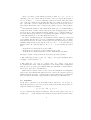
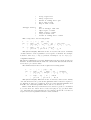
Let U denote a universe of ground terms formed only from c ∈ C and f ∈ F.
Given interpretations ρ and σ for predicate symbols and terms, respectively, we
define the satisfaction relations
(ρ, σ) |= pre and (ρ, σ) |= cl
for pre-conditions and clauses as in Table 1. Here we write ρ(R) for the set of
k-tuples (a1 , · · · , ak ) from U associated with the k-ary predicate R, and we write
2
σ(t) for the ground term of U bound to t with σ(c) = c for the constants, and
σ(f (t1 , ..., tk )) = f (σ(t1 ), ..., σ(tk )) for the functional terms. Further σ[x 7→ a]
stands for the mapping that is as σ except that x is mapped to a, and as a
particular case σ[cnt 7→ 1+ ] stands for the mapping that is as σ except that the
value of the integer variable cnt is increased by 1.
(ρ, σ) |= R (t1 , · · · , tk )
(ρ, σ) |= ¬R (t1 , · · · , tk )
(ρ, σ) |= pre1 ∧ pre2
(ρ, σ) |= pre1 ∨ pre2
(ρ, σ) |= ∃x : pre
(ρ, σ) |= t1 = t2
(ρ, σ) |= t1 6= t2
iff
iff
iff
iff
iff
iff
iff
(σ(t1 ), · · · , σ(tk )) ∈ ρ(R)
(σ(t1 ), · · · , σ(tk )) 6∈ ρ(R)
(ρ, σ) |= pre1 and (ρ, σ) |= pre2
(ρ, σ) |= pre1 or (ρ, σ) |= pre2
(ρ, σ[x 7→ a]) |= pre for some a ∈ U∗
σ(t1 ) = σ(t2 )
σ(t1 ) 6= σ(t2 )
(ρ, σ) |= R (t1 , · · · , tk )
(ρ, σ) |= 1
(ρ, σ) |= cl1 ∧ cl2
(ρ, σ) |= pre ⇒ cl
(ρ, σ) |= pre =⇒ cl
(ρ, σ) |= ∀x : cl
iff
iff
iff
iff
iff
iff
(σ(t1 ), · · · , σ(tk )) ∈ ρ(R)
true
(ρ, σ) |= cl1 and (ρ, σ) |= cl2
(ρ, σ) |= cl whenever (ρ, σ) |= pre
(ρ, σ[cnt 7→ 1+ ]) |= cl whenever (ρ, σ) |= pre
(ρ, σ[x 7→ a]) |= cl for all a ∈ U∗
Table 1. Semantics of pre-conditions and clauses
We view also the free variables occurring in a formula as ground terms from
the universe U. Thus, given an interpretation σ0 of the ground terms, in the
clause cl, we call an interpretation ρ of the predicate symbols R a solution to
the clause provided (ρ, σ0 ) |= cl. We use U∗ to denote the least subset of U such
such that U∗ ⊇ =ρ(R) given that =ρ(R) = {a1 , ..., ak : (a1 , ..., ak ) ∈ ρ(R)} for all
R ∈ R.
It needs to mention that the solver only terminates with a least solution iff
the least solution is finite.
Example 2. Let N at be a 1-ary predicate defining a natural number. The following formula define all the natural numbers:
N at(zero) ∧ ∀x : N at(x) ⇒ N at(succ(x))
where function succ computes the successor of a natural number. The least
solution to this formula is the infinite set IN of natural numbers. In this case the
solver will not terminate.
2
Download and install the solver
The zip file for the solver can be downloaded from:
3
http://www.imm.dtu.dk/cs/Secure/SuccinctSolver
You can then unzip the file under the directory you wish. The sources of the
solver are under the directory HORN after you have unziped the file.
3
User interfaces
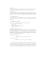
The structure FormulaAnalyzer described in the file formulaAnalyzer.sml in the
Formulas directory is an application of the functor FrontBackEnd which defines
the functions for users to access the solver. The functor FrontBackEnd is defined
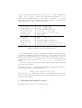
in the file frontBackEnd.sml in the same directory. The user interface provided
by FrontBackEnd is summarized in Table 2.
The functions given in the Table 2 can be classified into four groups including
the functions for initialization, the functions for input, functions for solving
clauses, and the functions for output. The initialization functions init and init1
are used to initialize all the global data structures which are used by the solver to
construct the solution. These data structures should be initialized before calling
the functions for solving clauses. The difference between these two functions is
that the former creates and returns the initialized data structure result (of type
Forest.forest), while the latter takes the result data structure as the input and
initialize it. In the following subsections, we shall describe the functions of the
other three groups.
3.1
Functions for input
There are four ways to input ALFP clauses to the solver:
–
–
–
–
input
input
input
input
from
from
from
from
SML data structures
a text file
stdIn (standard input)
a string
inputData clause
The function inputData receives the ALFP clause represented by the SML data
structure defined in the structure HornDirect. It then transforms the clause into
the internal data structure that the solver uses to process the clause.
The structure HornDirect, in the file hornDirect.sml under the directory
Formulas defines the following SML data structures to express ALFP clauses:
datatype term
=
|
|
Cons of string
Var of string
AppF of string * term list
datatype pre
=
|
Prel of string * term list
Nrel of string * term list
4
val init : unit -> Forest.forest
val init1: Forest.forest -> unit
val
val
val
val
val
inputData : HornDirect.clause -> HornPlus.clause list
inputFile : string -> HornPlus.clause list
inputStd : unit -> HornPlus.clause list
inputStr : string -> HornPlus.clause list
fromALFPtoHD : string -> HornDirect.clause list
val outputData : Forest.forest ->
(StringItem.item * IntItem.item) list * bool
-> string list * (string * string list list)
val outputFile : Forest.forest * string ->
(StringItem.item * IntItem.item) list * bool ->
val outputStd : Forest.forest ->
(StringItem.item * IntItem.item) list * bool ->
val outputStr : Forest.forest ->
(StringItem.item * IntItem.item) list * bool ->
list
unit
unit
string
val solve : Forest.forest * HornPlus.clause list -> unit
val solveCount : Forest.forest * HornPlus.clause list -> unit
val solveData : Forest.forest * HornPlus.clause list
-> string list * (string * string list list) list
val solveFile : Forest.forest * HornPlus.clause list * string -> unit
val solveStd : Forest.forest * HornPlus.clause list -> unit
val solveStr : Forest.forest * HornPlus.clause list -> string
val selectSolveData : Forest.forest * HornPlus.clause list ->
(StringItem.item * IntItem.item) list * bool * bool
-> string list * (string * string list list) list
val selectSolveFile : Forest.forest * HornPlus.clause list * string ->
(StringItem.item * IntItem.item) list * bool * bool
-> unit
val selectSolveStd : Forest.forest * HornPlus.clause list ->
(StringItem.item * IntItem.item) list * bool * bool
-> unit
val selectSolveStr : Forest.forest * HornPlus.clause list ->
(StringItem.item * IntItem.item) list * bool * bool
-> string
Table 2. Interface provided by FrontBackEnd
5
|
|
|
|
|
datatype clause =
|
|
|
|
|
Pconj of pre list
Pdisj of pre list
Exists of string list * pre
Eq of term * term
Neq of term * term
One
Rel of string * term list
Impl of pre * clause
BImpl of pre * clause
Conj of clause list
Forall of string list * clause
This corresponds to the following syntax:
t
pre
::=
::=
|
a | x | f (t1 , · · · , tk )
R (t1 , · · · , tk ) | ¬R (t1 , · · · , tk )
pre1 ∨ pre2 | ∃x1 , · · · , xk : pre
cl
::=
|
R (t1 , · · · , tk ) | 1 |
pre ⇒ cl | pre =⇒ cl
|
|
pre1 ∧ pre2
t1 = t2 | t1 6= t2
cl1 ∧ cl2
| ∀x1 , · · · , xk : cl
This syntax is slightly different from the one described in section 1.1 mainly
on that it allows to write a quantifier over a sequence of variables. For example,
it allows to write ∀x, y, z : P (x, y, z) instead of writing ∀x : ∀y : ∀z : P (x, y, z).
inputFile fileName
The function inputFile receives the ALFP clause from the text file specified by
fileName. It then transforms the clause into the internal data structure that the
solver uses to process the clause.
The ALFP clauses in the text file requires the following syntax:
t
pre
::=
::=
|
c | x | f (t1 , · · · , tk )
R (t1 , · · · , tk ) | !R (t1 , · · · , tk ) | pre1 &pre2
pre1 | pre2 | E x.pre | t1 = t2 | t1 ! = t2
cl
::=
|
R (t1 , · · · , tk ) | 1 |
pre ⇒ cl | pre =⇒ cl
cl1 &cl2
| A x.cl
This syntax is slightly different from the one introduced in section 1, mainly
on notations used for the operators and quantifiers. Here ! is used for negation, |
for disjunction, and & for conjunction. A in A x. is the universal quantifier, and
E in E x. the existential quantifier. The notation != is used for 6=.
Note: A and E are key tokens in the solver, therefore, please be careful and
do not use these two letters alone for any other purpose (e.g. predicate name
etc.). Otherwise the parser will raise the error message. Please also note there is
a space in between a quantifier and the bounded variable.
6
inputStd
The function inputStd receives the ALFP clause from the standard input, known
as stdIn, and then transforms the clause into the internal data structure.
inputStr str
The function inputStr receives the ALFP clause from the string str, and transforms the clause into the internal data structure. This is mainly used for receiving
the clause via sockets by means of the SML/NJ Socket structure (cf. Appendix
A).
fromALFPtoHD fileName
The auxiliary function fromALFPtoHD is used to transform the ALFP clause
in the text file specified by fileName to the SML data structure defined in
HornDirect.
3.2
Functions for output
There are also four ways to output the result from the solver:
–
–
–
–
output
output
output
output
to
to
to
to
SML data structures
a file
stdOut (standard output)
a string
outputData result, (select, univ)
The function outputData is used to output the result to a SML data structure
with the type string list * (string * string list list) list. The first
list represents the universe, i.e. a list of ground terms, each is represented by a
string. The second list represents the result, which contains a list of relations.
Each relation is represented by a relation name (of string type), and a list of
tuples of ground terms (string list list).
Example 3. The relation
SIST ERS : (Ann, M ary), (Susan, Hellen)
is represented by a list:
[“SISTERS”, [[“Ann”, “Mary”], [“Susan”, “Hellen”]]]
.
The function has three parameters: result, select, and univ. The result (of
type Forest.forest) holds the solution from the solver. The select (of type (string
* int) list) specifies a list of relations as the output. A relation is represented
by a pair of the relation name, and its arity. For example, if one is going to
output the 2-ary relation SIST ERS from the result, the select is specified by
7
[(“SISTERS”, 2)]. The empty list corresponds to selecting all the relations as
the output. The univ specifies whether or not the universe is also included as
the output. If it is true, the universe is output as well. If it is false the universe
is excluded from the output.
outputFile (result, fileName) (select, univ)
The function outputFile is used to output the result to a text file. The function has four parameters: result, fileName, select, and univ. The fileName specifies the output file name. The result, select and univ are the same as those in
outputData.
outputStd result (select, univ)
The function outputFile is used to output the result to stdOut, i.e. the standard output. The three parameters: result, select, and univ are the same as those
in outputData.
outputStr result (select, univ)
The function outputFile is used to output the result to a string. The three
parameters: result, select, and univ are the same as those in outputData. Again,
this function is mainly used for sending the result via sockets by means of the
SML/NJ Socket structure (cf. Appendix A).
3.3
Functions for solving
There are ten functions in this group. Two of them (solve and solveCount) are
used to solve the clause represented by the internal data structure and construct
the solution to the clause in the result data structure, without output of the
result. The other functions combine these two functions with different output
functions to easy the user to output the result.
solve (result, cl)
The function solve is used to solve the clause without the output of the result.
This can be used in an iterative solving process where the intermediate result is
not of interests, and the final result can be output using the functions for output.
The solve function has two parameters: result and cl. The result holds the
global data structure containing the solution to the clause, and the cl is the
clause (generated by an input function) that is going to be solved. These two
parameters are used in all the following functions, and we shall not describe
them again in the sequel, if there no special purpose.
solveCount (result, cl)
The function solveCount is essentially the same as solve, but printing a summary of the result, e.g. the universe, the number of elements for each relation,
and etc., onto the screen.
solveData (result, cl)
8
The function solveData is used to solve the clause and output all the result
including the universe in the way that outputData does. At the same time it
prints a summary of the result onto the screen.
solveFile (result, cl, fileName)
The function solveFile is used to solve the clause and output all the result including the universe to the file specified by fileName. At the same time it prints
a summary of the result onto the screen.
solveStd (result, cl)
The function solveStd is used to solve the clause and output all the result including the universe to the standard output stdOut. At the same time it prints
a summary onto the screen.
solveStr (result, cl)
The function solveStd is used to solve the clause and output all the result including the universe to a string, which will be returned. At the same time it
prints a summary onto the screen.
selectSolveData (result, cl) (select, univ, count)
The function selectSolveData is used to solve the clause and output the selected the result in the way that outputData does. It has five parameters. The
parameters result and cl are the same as those in solve, while select and univ
are the same as those in outputData. The count is used to specify whether a
summary of the result is printed or not. If it is true, the summary of the result
is printed, otherwise the summary is not printed.
selectSolveFile (result, cl, fileName) (select, univ, count)
The function selectSolveFile is used to solve the clause and output the the
selected result to the file specified by fileName. The other parameters are the
same as those in selectSolveData.
selectSolveStd (result, cl) (select, univ, count)
The function selectSolveStd is used to solve the clause and output the selected
result to the standard output stdOut.
selectSolveStr (result, cl) (select, univ, count)
The function selectSolveStr is used to solve the clause and output the selected
result as a string returned.
3.4
Other facilities
We provide also some other auxiliary functions to facilitate the use of the solver.
As we have already mentioned that the structure HornDirect defines the SML
data structure to represent ALFP clauses. It provides also a function called
translate to translate a clause from HornDirect data structure to the solver’s
9
internal representation of clauses and thus avoiding the ALFP’s parser. Symmetrically, we also provide a structure called InternToDirect, in the file internToDirect.sml under the directory Formulas, where a function called toHdClause is to
transform a clause resulted from the parser into the HornDirect data structure.
In addition, we provide the following facilities:
Pretty print. The structure Pretty, defined in the pPrint.sml file under the
directory Formulas, provides three functions to print clauses defined in the
HornDirect structure into a Latex file so that one can include it into the Latex
document whenever there is a need. The interface to these functions are:
val prettyTable : string ∗ clause ∗ string →
val prettyFrame : string ∗ clause → unit
val prettyText : string ∗ clause → unit
unit
prettyTable (fname, cl, capt)
The function prettyTable is used to print the clause cl into the Latex file called
fname.tex as a framed table, and the string capt is the contents of the caption of
the table. Moreover, fname is also used as a label of the table for your reference
in your Latex document.
prettyFrame (fname, cl)
The function prettyFrame is used to print the clause cl into the Latex file called
fname.tex as a framed text.
prettyText (fname, cl)
The function prettyText is used to print the clause cl into the Latex file called
fname.tex as a pure text without any decoration.
When the file fname.tex is included in the main Latex document, the alfp.sty
file should also be included. The alfp.sty file is in the Application directory.
As mentioned in the previous section, the function fromALFPtoHD is used to
transform the ALFP clause from the text file to the clause represented by the
HornDirect structure. One can therefore use the pretty print function to print
the ALFP clause from the text file as well.
Making a breakpoint. As mentioned, the clause pre =⇒ cl is used to make
a breakpoint in front of clause cl in order to print the number of environments
passing through the breakpoint of clause cl. Intuitively, it gives how many times
the clause cl will be executed. In the solver, the (partial) environment is used
to map variables to the ground terms from the universe [1]. The experiments
with the solver in [2] reports that minor syntactical variations of formulas, e.g.
the order of conjuncts in preconditions, have a strong impact on computation
efficiency of the solver.
It is often not easy to predicate which order of the conjuncts in preconditions
is better than the others, which depends on the current environment that the
unification is carried on and the values to be unified.
10
Example 4. Consider a fragment P1 (x, y) ∧ P2 (x, y) ⇒ Q(x, y) of a clause, where
x and y are bounded variables. When the precondition P1 (x, y) ∧ P2 (x, y) is
checked, variable x is e.g. binded by constant a, and y is not yet binded in the
current environment. The solver makes first the query to the predicate P1 and
obtains a list of tuples for P1 , and it then unifies each tuple with the current
environment. Each successful unification will produce a new environment for P2
to be checked. If e.g. the list of tuples for predicate P1 is [(a, b), (a,c), (a,d)],
and after the query to P1 is done, it produces three environments. The query to
P2 is then carried out in three environment. If e.g. the list tuples for predicate
P2 is [(b, b), (b,c), (b,d)], it is easy to see that all the unifications will be failed.
Therefore no execution to assertion Q(x, y). In this case, if we could check P2
first then we would not check P1 and save unnecessary computation expenses.
In this situation, e.g., one can use the clause pre =⇒ cl to replace the
clause pre ⇒ cl in order to do some debugging, e.g. with different orderings in
preconditions.
Example 5. Consider the clause ∀x : ∀y : P1 (x, y) ∧ P2 (x, y) ⇒ Q(x, y), we can
do the followings:
1. Transform the clause into: ∀x : ∀y : P1 (x, y) =⇒ (P2 (y, x) ⇒ Q(x, y)), and
run the solver. When the computation is done, we will see a message from
the screen “Number of env’s passing through the breakpoint: n1 ”, where the
number n1 tells you how many times that the clause P2 (y, x) ⇒ Q(x, y) is
going to be executed.
2. Transform the clause into: ∀x : ∀y : P1 (x, y) =⇒ (P2 (x, y) ⇒ Q(x, y)),
repeat the same procedure as in (1) and we obtain the number n2
3. We then may be able to choose the order by n1 and n2 . We shall choose the
order that precondition producing the smaller number precedes the precondition producing the larger number.
4
Run the solver
In general one can use the functions described above to easily construct a function to run the solver according to one’s own needs. However, we provide three
files called run, reRun and reRunSock to facilitate to run the solver. The functions in the file run are used to run the solver once for each single application.
The functions in the file reRun are used to run the solver iteratively through the
interactions with the solver. In both cases, the input clause is from a text file.
The functions in the file reRunSock are used to run the solver as a Web server
process using sockets. One may also use these files as frameworks to construct
one’s own run functions. There three files are in the sub-directory called Application, which one may change its name, under the HORN directory. In the
followings we briefly describe how to use the functions in these three files.
11
4.1
The run file
The run file contains two functions, ex and exs. The function ex has one parameter fname which gives the input file name without the suffix. It solves the
clause from the file fname.cl and output all the result including the universe to
the file fname.cl.al. At the same time it prints a summary of the result onto the
screen.
The function exs has three parameters: fname, select, and univ. The fname
is the same as that in the function ex, the select and univ are the same as the
parameters for the output functions that we have discussed in section 3.2. It
solves the clause from the file fname.cl and output the selected result to the file
fname.cl.al. At the same time it prints a summary of the result onto the screen.
Under the directory Application, there is a sub-directory called Examples,
which one should not change its name (if not modify the run file. The text file
containing the ALFP clauses should be put in the Examples directory, and the
file name should have a suffix .cl. For example, if a clause is in the file called
myfile.cl, we then use the ex function in the following steps:
1.
2.
3.
4.
Go to the Application directory, start sml
Under the sml prompt, input command: use “run”;
After the solver is compiled, run the solver by input: ex(“myfile”);
The solver generates an output file called myfile.cl.al in the directory Examples
The exs function is used in the same way, but with extra arguments.
4.2
The reRun file
The reRun file contains two functions, ex and exs. The function ex has no
parameter. It interacts with the user to ask the user to specify the file (i.e. input
the file name fname without the suffix) which contains the clause. It then calls
the function to solve the clause from the file fname.cl and output the all result
including the universe to the file fname.cl.al. It prints also a summary of the
result onto the screen.
The function exs has one parameteruniv to specify whether or not the universe is included in the output, as we have mentioned in section 3.2. It interactively asks the user to input the file name fname and the selected output select.
The input format for select is the same as the parameter select that we have
discussed in section 3.2. It then calls the function to solve the clause from the
file fname.cl and output the selected result to the file fname.cl.al. It prints also
a summary of the result onto the screen.
Assume that the clause to be solved is in the file called myfile.cl under the
sub-directory Examples, we then use the ex function in the following steps:
1. Go to your Application directory, start sml
2. Under the sml prompt, input command: use “reRun”;
3. After the solver is compiled, run the solver by input: ex();
12
4. The solver prompts to us by “Please enter a file name ! (cr for exit)”. We
then enter the file name myfile (without suffix). The solver solves the clauses
in the file, and outputs the result in the file called myfile.cl.al. The solver
will repeat the same prompt to us and ask for the new input
5. If we wish to solve another clause by querying the result from the previous
run, we just input the new file’s name as before, otherwise we terminate the
current run by entering a Return key
The exs function is used in the same way, but with more interactions.
4.3
The reRunSock file
The reRunSock file contains functions to run the solver as a Web server process
for a Web client/server application. It uses the SML/NJ Socket structure to
implement the socket communication between the solver and the client, i.e. a
web browser. The function serve provides services to the client using sockets.
The serve can deal with three commands: “openf”, “close” and “solve”.
When the command “openf” is received, the serve calls the solveFile
function to solve the clause in a text file specified by the next received message. When the command “close” is received, the serve terminates the current
solving and initializes all the global data structures ready for the next solving.
When the command “solve” is received, the serve function calls the inputStr
and selectSolveStr functions to transform a clause from the string received
from the socket into the internal representation and solve the internal represented clause with the selected output to a string which will be send back via
the socket to the client.
Another function called main is used to generate the heap image of the solver.
The heap image for Windows is called solver.x86-win32, and for Linux is called
solver.x86-linux (both have been generated and saved in the sub-directory Application. One can run the saved image by input e.g. in Windows:
sml@SM Lload = solver.x86 − win32
In Appendix A, we present a framework of the Web browser (contributed by
Terkel Tolstrup) which uses the solver as a server process.
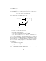
Appendix A. Presenting the results of the solver through
a web browser
This section will give a framework for presenting results of the solver through
a web browser. The framework includes functions for communicating with the
Succinct Solver using the socket interface (cf. section 4.3). The framework is
implemented in ML Server Pages, so a webserver, for example the Apache HTTP
server project:
http://httpd.apache.org/
13
and the MSPCompile:
http://ellemose.dina.kvl.dk/˜sestoft/msp/index.msp
is required. Furthermore the libraries expected in the framework must be implemented in Standard ML (and compiled using Moscow ML:
http://www.dina.dk/˜sestoft/mosml.html.
This framework is meant as an example of an application using the Succinct
Solver and presenting the result through a browser.
Scanner/Parser
Constraint generator
Succinct Solver
Pretty-Printer
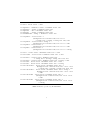
Result
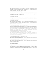
Fig. 1. Architecture of the framework
The framework consist of three major parts:
– An analysis part, parsing input and generating predicates for the solver with
regards to the analysis performed.
– A pretty printer, presenting the parsed input as HTML.
– A result generator, feeding a predicate to the solver corresponding to the
interaction from the user.
Analysis part: The analysis part can be implemented using Lex and Yac (as
shown in Whi2cllex.lex and Whi2clpar.grm for the WHILE language, parsing
is done by the functions in Whi2cl.sml). Furthermore functions for generating
the predicates for the analysis performed is needed. The predicates is written to
a file in the Examples directory, and passed to the Succinct Solver in the lines:
val parsfil =
parsef (hd(part_field_strings
(valOf (cgi_part "FileName")) "filename"))
val labprog = W.AddLabel parsfil
val _ =
W.outputfile (W.GenConst labprog, "Examples/" ^ profnm ^ ".cl");
val _ = sendSock 9000 ["openf", profnm] false
14
Pretty printer part: The pretty printed program text is displayed in the top
frame (prettyprinter.msp).
Here the file is parsed from the local machine using the parsef function (from
Whi2cl.sml), then predicates for the Reaching Definitions analysis is generated
and written to a file. Finally a command for opening and solving the file is send
on socket 9000 to the Succinct Solver.
If you want to parse a file from another machine the following line can replace
the previous:
val parsfil = parses (part_data (valOf (cgi_part "FileName")))
Have in mind that the inputs to the solver will be mixed if concurrent processes of the website are invoked. This framework is meant as a single user
application.
The parsed file is pretty printed:
prettyPrint labprog profnm
The function prettyPrint is found in PP.sml, it prints programs in the
WHILE language as HTML with hyperlinks to the result frame. The following
function pretty prints arithmetic expressions as HTML, making all variables link
to the result of the Reaching Definitions analysis:
fun printAexp (W.CstR r)
Real.toString r
fnm =
| printAexp (W.Var v)
fnm =
"<a href=\"result.msp?prog="^fnm^"&variable="^v^"\"
target=\"result\">"^v^"</a>"
| printAexp (W.Plus (a1,a2)) fnm =
printAexp a1 fnm ^ " + " ^ printAexp a2 fnm
| printAexp (W.Minus (a1,a2)) fnm =
printAexp a1 fnm ^ " - " ^ printAexp a2 fnm
| printAexp (W.Times (a1,a2)) fnm =
printAexp a1 fnm ^ " * " ^ printAexp a2 fnm
| printAexp (W.Divide (a1,a2))fnm =
printAexp a1 fnm ^ " / " ^ printAexp a2 fnm
Result generator part: The result generator is displayed in a frame below the
one displaying the pretty printed program. It will receive information about the
variable or label clicked in the program text as CGI fields.
The result.msp reacts on the received CGI fields and sends a corresponding
predicate to the solver:
15
val _ =
(case cgi_field_string "variable" of
NONE
=> ()
| SOME(vari) =>
(sender ["solve",
"A l1. A l2. RDOUT(l1,"^vari^",l2) => RD" ^ vari ^
"(l1,l2)", "RD"^ vari, "2"]
true)
)
The result is received from the solver and displayed in the frame. Notice
the format of the solve command send to the Succinct Solver is in the format
["solve", result-predicate , name-of-relation , arity-of-relation ].
The framework packages can be found at:
http://www.imm.dtu.dk/cs/Secure/SuccinctSolver.
It includes the files describe in this section. To try the running version the files
of the packages must be placed in the htdocs/ directory of the Apache Server
installation. The function libraries must be compiled (using MOSMLC, MOSMLLEX and MOSMLYAC). Remember to set the environment variable MOSMLLIB to include the htdocs/ directory, and set the file/directory permissions to
allow access through the Apache Server.
References
[1] F. Nielson, H. Seidl, and H. Riis Nielson. A Succinct Solver for ALFP, Nodic journal
for computing, (9)2002, 2002.
[2] M. Buchholtz, H. Riis Nielson, and F. Nielson. Experiments with Succinct Solvers.
Technical Report IMM-TR-2002-4, IMM, DTU, 2002.
[3] H. Sun, H. Riis Nielson, and F. Nielson. Data Structures in the Succinct Solver
(V1.0). Technical Report IMM-SECSAFE-005, 2002.
[4] H. Sun, H. Riis Nielson, and F. Nielson. Extended Features in the Succinct Solver
(V2.0). Technical Report IMM-SECSAFE-009, 2003.
16